Pattern Recognition Letters 49 (2014) 146–154

Contents lists available at ScienceDirect

Pattern Recognition Letters

journal homepage: www.elsevier .com/locate /patrec

Chronological classification of ancient paintings using appearanceand shape features q

http://dx.doi.org/10.1016/j.patrec.2014.07.0020167-8655/� 2014 Elsevier B.V. All rights reserved.

q This paper has been recommended for acceptance by Jie Zou.⇑ Corresponding author. Tel.: +86 27 68775721; fax: +86 27 68778035.

E-mail addresses: qinnzou@gmail.com (Q. Zou), cao@cec.sc.edu (Y. Cao),qqli@whu.edu.cn (Q. Li), huangch@whu.edu.cn (C. Huang), songwang@sc.edu(S. Wang).

Qin Zou a,⇑, Yu Cao b, Qingquan Li c, Chuanhe Huang a, Song Wang b

a School of Computer Science, Wuhan University, Wuhan 430072, PR Chinab Department of Computer Science and Engineering, University of South Carolina, Columbia, SC 29208, USAc Shenzhen Key Laboratory of Spatial Information Smart Sensing and Service, Shenzhen University, Guangdong 518060, PR China

a r t i c l e i n f o

Article history:Received 26 November 2013Available online 23 July 2014

Keywords:Painting classificationPainting style analysisDeep learningImage classification

a b s t r a c t

Ancient paintings are valuable for historians and archeologists to study the humanities, customs andeconomy of the corresponding eras. For this purpose, it is important to first determine the era in whicha painting was drawn. This problem can be very challenging when the paintings from different eraspresent a same topic and only show subtle difference in terms of the painting styles. In this paper, wepropose a novel computational approach to address this problem by using the appearance and shape fea-tures extracted from the paintings. In this approach, we first extract the appearance and shape featuresusing the SIFT and kAS descriptors, respectively. We then encode these features with deep learning in anunsupervised way. Finally, we combine all the features in the form of bag-of-visual-words and train aclassifier in a supervised fashion. In the experiments, we collect 660 Flying-Apsaras paintings from MogaoGrottoes in Dunhuang, China and classify them into three different eras, with very promising results.

� 2014 Elsevier B.V. All rights reserved.

1. Introduction

Ancient paintings have provided valuable sources for historiansand archeologist to study the history and humanity at the corre-sponding eras. Fig. 1 displays four painting images collected fromMogao Grottoes in Dunhuang, China. These four paintings werecreated in different eras of China, namely the Wudai dynasty, theSui dynasty, and the peak Tang dynasty, respectively. From thesepaintings, we can find a lot of important information in the corre-sponding eras, e.g., the architecture style in the Wudai dynastyfrom Fig. 1(a), the musical instruments in the Sui dynasty fromFig. 1(b), the plowing manner of farmers in the peak Tang dynastyfrom Fig. 1(c), and the costumes in the peak Tang dynasty fromFig. 1(d).

Obviously, a very important problem is to correctly determinethe era in which a painting was created. Usually it is unreliableto determine the painting era based only on the specific contentof the painting, since one same topic may be presented in thepaintings in different eras. As widely adopted in art appraisal,people usually determine the era of a painting by examining its

painting style, which usually varies with time and shows subtledifferences from one era to another. It is usually difficult, if noimpossible, for the general people without special training onpainting and painting history to identify such subtle variation ofthe painting style for correctly determining the era of a painting.In this paper, our goal is to develop an automatic, computationalapproach to address this problem by using both appearance andshape features. Together with a supervised learning, we expectthat the proposed approach can implicitly capture the specificpainting style in different eras for painting-image classification.

To better capture the painting style implied in the paintings, wefocus on the paintings created in different eras, but presenting thesame topic. An example is shown in Fig. 2, where all 12 paintingimages present the Flying Apsaras, an important theme of thepaintings of Mogao Grottoes in Dunhuang, China. These 12 paint-ings were created in different periods of Dunhuang Art: the infancyperiod (Row 1), the creative period (Row 2), and the mature period(Row 3). From these sample images, we can see that the painting-style difference in these three periods are subtle and only expertson Chinese classic art may be able to distinguish them. In thispaper, we develop our automatic approach to localize such subtledifference and correctly determine the eras for such paintings.

Besides the appearance features, one interesting observation isthat, each flying fairy in the Flying-Apsaras painting wears scarves,and it seems that the shape of the scarves varies from one period toanother. An example is shown in Fig. 3. In the infancy period of the

Fig. 1. Sample paintings from different eras. (a) A painting in Wudai dynasty (907–960) from Mogao Grottoes 61, (b) a painting in Sui dynasty (581–618) from MogaoGrottoes 285, (c) a painting in peak Tang dynasty (712–762) from Mogao Grottoes 23, (d) a painting in peak Tang dynasty (712–762) from Mogao Grottoes 45.

Fig. 2. Sample paintings with the same topic but created in different eras. Row 1: four paintings created at the infancy period of the Flying-Apsaras art (421–556), Row 2: fourpaintings created at the creative period of the Flying-Apsaras art (557–618), Row 3: four paintings created at the mature period of the Flying-Apsaras art (619–959).

Q. Zou et al. / Pattern Recognition Letters 49 (2014) 146–154 147

Flying-Apsaras art, line and curve strokes sketching the scarves arerelatively simple and flat, as shown in Fig. 3left). In the creativeperiod, scarves are sketched with small waves, as shown inFig. 3middle). While in the mature period, scarves as well as cloudsare more wavy than in the early periods, as shown in Fig. 3right). Inthis work, the main hypothesis is that the painting style can bedescribed by the local appearance and shape features extractedfrom the painting images. This way, the difference of paintingstyles in different eras can be captured by learning from a set oftraining image samples. Based on this hypothesis, the proposedapproach consists of the following steps: (1) appearance and shapefeatures are extracted using the Scale-Invariant Feature Transform(SIFT) [21] and kAS shape description [7], (2) appearance featuresare further encoded by a deep-learning algorithm to enhance therepresentation abstraction ability, (3) visual codebooks are con-structed based on the encoded appearance features and shape fea-tures, (4) feature histograms are produced for each painting as theinput of the classifier, (5) training a classifier in a supervised fash-ion to determine the era of a painting based on the above featurehistogram. In the experiments, we collect 660 Flying-Apsaras paint-ings from Mogao Grottoes in Dunhuang, China and classify theminto either the infancy period, the creative period, or the matureperiod as shown in Fig. 2.

There are two major contributions in this paper. First, wedeveloped a feature detection/combination method that can

distinguish the subtle difference of the Dunhuang Flying-Apsaraspaintings from different eras. We found that both appearance fea-tures and shape features are important for this classification task,which is consistent with the opinions of the art experts onDunhuang paintings. Second, we proposed to use, in an originalway, the combination of a typical set of image features (SIFT, animage-gradient based feature that are scale and rotation invari-ant) with one of the most effective feature refinementalgorithms (deep learning, a specific type of Boltzmann machines).In the experiments, we compared the proposed method to arecent state-of-the-art painting classification method, with aclearly better performance.

The remainder of this paper is organized as follows. Section 2introduces the related work. Section 3 presents our approach forextracting the appearance and shape features. Section 4 reportsour experiment results on 660 Flying-Apsaras paintings and Sec-tion 5 concludes the paper.

2. Related work

As a branch of the image classification/retrieval research, paint-ing classification has attracted more and more attention in the pasttwo decades [26,17,28,29,15,8]. Existing painting-classificationresearches are usually focused on two applications, classifying

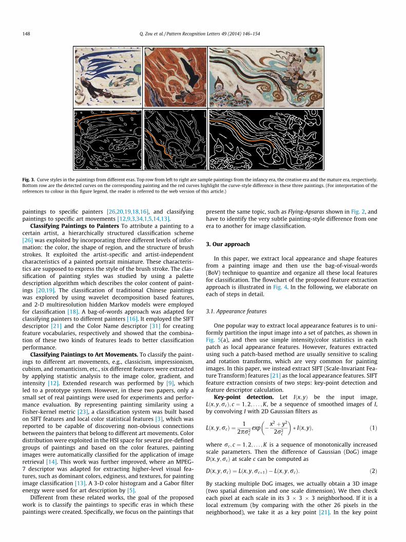
Fig. 3. Curve styles in the paintings from different eras. Top row from left to right are sample paintings from the infancy era, the creative era and the mature era, respectively.Bottom row are the detected curves on the corresponding painting and the red curves highlight the curve-style difference in these three paintings. (For interpretation of thereferences to colour in this figure legend, the reader is referred to the web version of this article.)

148 Q. Zou et al. / Pattern Recognition Letters 49 (2014) 146–154

paintings to specific painters [26,20,19,18,16], and classifyingpaintings to specific art movements [12,9,3,34,1,5,14,13].

Classifying Paintings to Painters To attribute a painting to acertain artist, a hierarchically structured classification scheme[26] was exploited by incorporating three different levels of infor-mation: the color, the shape of region, and the structure of brushstrokes. It exploited the artist-specific and artist-independentcharacteristics of a painted portrait miniature. These characteris-tics are supposed to express the style of the brush stroke. The clas-sification of painting styles was studied by using a palettedescription algorithm which describes the color content of paint-ings [20,19]. The classification of traditional Chinese paintingswas explored by using wavelet decomposition based features,and 2-D multiresolution hidden Markov models were employedfor classification [18]. A bag-of-words approach was adapted forclassifying painters to different painters [16]. It employed the SIFTdescriptor [21] and the Color Name descriptor [31] for creatingfeature vocabularies, respectively and showed that the combina-tion of these two kinds of features leads to better classificationperformance.

Classifying Paintings to Art Movements. To classify the paint-ings to different art movements, e.g., classicism, impressionism,cubism, and romanticism, etc., six different features were extractedby applying statistic analysis to the image color, gradient, andintensity [12]. Extended research was performed by [9], whichled to a prototype system. However, in these two papers, only asmall set of real paintings were used for experiments and perfor-mance evaluation. By representing painting similarity using aFisher-kernel metric [23], a classification system was built basedon SIFT features and local color statistical features [3], which wasreported to be capable of discovering non-obvious connectionsbetween the painters that belong to different art movements. Colordistribution were exploited in the HSI space for several pre-definedgroups of paintings and based on the color features, paintingimages were automatically classified for the application of imageretrieval [14]. This work was further improved, where an MPEG-7 descriptor was adapted for extracting higher-level visual fea-tures, such as dominant colors, edginess, and textures, for paintingimage classification [13]. A 3-D color histogram and a Gabor filterenergy were used for art description by [5].

Different from these related works, the goal of the proposedwork is to classify the paintings to specific eras in which thesepaintings were created. Specifically, we focus on the paintings that

present the same topic, such as Flying-Apsaras shown in Fig. 2, andhave to identify the very subtle painting-style difference from oneera to another for image classification.

3. Our approach

In this paper, we extract local appearance and shape featuresfrom a painting image and then use the bag-of-visual-words(BoV) technique to quantize and organize all these local featuresfor classification. The flowchart of the proposed feature extractionapproach is illustrated in Fig. 4. In the following, we elaborate oneach of steps in detail.

3.1. Appearance features

One popular way to extract local appearance features is to uni-formly partition the input image into a set of patches, as shown inFig. 5(a), and then use simple intensity/color statistics in eachpatch as local appearance features. However, features extractedusing such a patch-based method are usually sensitive to scalingand rotation transforms, which are very common for paintingimages. In this paper, we instead extract SIFT (Scale-Invariant Fea-ture Transform) features [21] as the local appearance features. SIFTfeature extraction consists of two steps: key-point detection andfeature descriptor calculation.

Key-point detection. Let Iðx; yÞ be the input image,Lðx; y;rcÞ; c ¼ 1;2; . . . ;K , be a sequence of smoothed images of I,by convolving I with 2D Gaussian filters as

Lðx; y;rcÞ ¼1

2pr2c

exp � x2 þ y2

2r2c

� �� Iðx; yÞ; ð1Þ

where rc; c ¼ 1;2; . . . ;K is a sequence of monotonically increasedscale parameters. Then the difference of Gaussian (DoG) imageDðx; y;rcÞ at scale c can be computed as

Dðx; y;rcÞ ¼ Lðx; y;rcþ1Þ � Lðx; y;rcÞ: ð2Þ

By stacking multiple DoG images, we actually obtain a 3D image(two spatial dimension and one scale dimension). We then checkeach pixel at each scale in its 3 � 3 � 3 neighborhood. If it is alocal extremum (by comparing with the other 26 pixels in theneighborhood), we take it as a key point [21]. In the key point

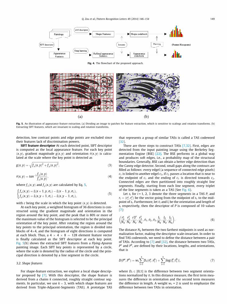
Fig. 4. The flowchart of the proposed approach.

Fig. 5. An illustration of appearance feature extraction. (a) Dividing an image to patches for feature extraction, which is sensitive to scalings and rotation transforms. (b)Extracting SIFT features, which are invariant to scaling and rotation transforms.

Q. Zou et al. / Pattern Recognition Letters 49 (2014) 146–154 149

detection, low contrast points and edge points are excluded sincetheir features lack of discrimination powers.

SIFT feature descriptor At each detected point, SIFT descriptoris computed as the local appearance feature. For each key pointðx; yÞ, gradient magnitude gðx; yÞ and orientation hðx; yÞ is calcu-lated at the scale where the key point is detected as

gðx; yÞ ¼ffiffiffiffiffiffiffiffiffiffiffiffiffiffiffiffiffiffiffiffiffiffiffiffiffiffiffiffiffiffiffiffiffiffiffiffiffiffiffiffif xðx; yÞ

2 þ f yðx; yÞ2

q; ð3Þ

hðx; yÞ ¼ tan�1 f yðx; yÞf xðx; yÞ

; ð4Þ

where f xðx; yÞ and f yðx; yÞ are calculated by Eq. 5,

f xðx; yÞ ¼ Lðxþ 1; y;rcÞ � Lðx� 1; y;rcÞ;f yðx; yÞ ¼ Lðx; yþ 1;rcÞ � Lðx; y� 1;rcÞ;

(ð5Þ

with c being the scale in which the key point ðx; yÞ is detected.At each key point, a weighted histogram of 36 directions is con-

structed using the gradient magnitude and orientation in theregion around the key point, and the peak that is 80% or more ofthe maximum value of the histogram is selected to be the principalorientation of the key point. After rotating the region around thekey points to the principal orientation, the region is divided intoblocks of 4�4, and the histogram of eight directions is computedat each block. Thus, a 4 � 4 � 8 ¼ 128 element feature vectoris finally calculated as the SIFT descriptor at each key point.Fig. 5(b) shows the extracted SIFT features from a Flying-Apsaraspainting image. Each SIFT key points is represented by a circle,where the scale is denoted by the radius of the circle and the prin-cipal direction is denoted by a line segment in the circle.

3.2. Shape features

For shape-feature extraction, we explore a local shape descrip-tor proposed by [7]. With this descriptor, the shape feature isderived from a chains k connected, roughly straight contour seg-ments. In particular, we use k ¼ 3, with which shape features arederived from Triple-Adjacent-Segments (TAS). A prototype TAS

that represents a group of similar TASs is called a TAS codeword[32].

There are three steps to construct TASs [7,32]. First, edges aredetected from the input painting image using the Berkeley Seg-mentation Engine (BSE) [22]. The BSE performs in a global wayand produces soft edges, i.e., a probability map of the structuralboundaries. Generally, BSE can obtain a better edge detection thanthe Canny edge detector. Second, small gaps along the contours arefilled as follows: every edgel (a sequence of connected edge pixels)c1 is linked to another edgel c2, if c2 passes a location that is near tothe endpoint of c1 and the ending of c1 is directed towards c2.Connected edges are then partitioned into roughly straight linesegments. Finally, starting from each line segment, every tripletof the line segments is taken as a TAS (See Fig. 6).

Let si for i = 1, 2, 3 denote the three segments in a TAS P, andri ¼ ðrx

i ; ryi Þ be the vector going from the midpoint of s1 to the mid-

point of si. Furthermore, let hi and li be the orientation and length ofsi respectively, then the descriptor of P is composed of 10 values[7]:

rx2

Nd;

ry2

Nd;r3x

Nd;

ry3

Nd; h1; h2; h3;

l1

Nd;

l2

Nd;

l3

Nd

� �: ð6Þ

The distance Nd between the two farthest midpoints is used as nor-malization factor, making the descriptor scale-invariant. In order tofind TAS codewords, we need to define the distance between a pairof TASs. According to [7] and [32], the distance between two TASs,Pa and Pb, are defined by their locations, lengths, and orientations,that is

DðPa; PbÞ ¼ wh

X3

i¼1

Dhðhai ; h

bi Þ þ

X3

i¼1

jlogðlai =lb

i Þj; ð7Þ

where Dh 2 [0,1] is the difference between two segment orienta-tions normalized by p. In this distance measure, the first term mea-sures the difference in orientation and the second term measuresthe difference in length. A weight wh = 2 is used to emphasize thedifference between two TASs in orientation.

Fig. 6. An illustration of shape feature extraction. (a) Edge probability map computed using the Berkeley Segmentation Engine. (b) Detected TASs, where each TAS isrepresented by a connected curve segment with the same color.

150 Q. Zou et al. / Pattern Recognition Letters 49 (2014) 146–154

3.3. SIFT feature refinement by deep learning

As a local appearance descriptor, SIFT is invariant to uniformscaling, and rotation. However, SIFT feature is sensitive to wideillumination variations and non-rigid transformations. In ancientpaintings, worn-out regions are frequently observed and suchregions can be viewed as strong illumination variations. Moreover,structural difference between two paintings, even for the twopaintings in the same era (see Fig. 2), are usually non-rigid. In thispaper, we use unsupervised deep learning to further refine theextracted SIFT features. This way, we utilize not only the scale/rotation invariance in the SIFT features, but also the representationabstraction ability of deep learning.

Deep learning [10,2,24] is motivated by the studies on visualcortex, which have revealed that the brain has a deep architectureand signals flow from one brain area (layer) to the next. Each layerof this feature hierarchy represents the input at a different level ofabstraction. Deep learning is a computational feature abstractionstrategy which simulates the function of the deep architecture ofbrain. In this paper, we use the popular deep belief networks(DBN) [10] for refining the SIFT features. Typically, the deep-learn-ing procedure of DBN consists of two stages: 1) abstracting infor-mation layer by layer and 2) fine-tuning the whole deep network[10]. In the first stage, DBN tunes the weights between two adja-cent layers by a family of Restricted Boltzmann Machines (RBMs)[25]. In the second stage, the weights in the whole deep networkare fine-tuned using a contrastive version of the wake-sleep algo-rithm [10,33]. The first stage is unsupervised, which is also referred

Fig. 7. An n-layer feature learning with RBMs. W and W 0 represent weights between the nand H1 to Hn are the hidden layers.

as feature learning, and the second stage is supervised, whichrequires the class labels for the input feature. In this paper, SIFTfeature points are detected without any class labels. Therefore,we only use the first stage of the DBN deep-learning procedure,i.e., the unsupervised feature learning, to refine the detected SIFTfeatures.

Without loss of generality, let us consider feature learningfrom a visible layer v to a hidden layer h, e.g., input feature layerH0 to a hidden layer H1 in Fig. 7(a). Each node represents a fea-ture dimension in its respective layer. Assuming all nodes arebinary random variables (0 or 1) and they satisfy the Boltzmanndistribution, the bipartite graph formed by connecting the nodesacross these two layers is a Restricted Boltzmann Machine(RBM).

In an RBM, a joint configuration of the visible and hidden unitshas an energy

Eðv ;h; hÞ ¼ �X

i;j

Wijv ihj �X

i

biv i �X

j

ajhj; ð8Þ

where h denotes the parameters (W; a; b), W denotes the weightsbetween visible and hidden units, a and b denote the bias of the hid-den layer and the visible layer, respectively. Then the probability ofthe joint configuration is given by the Boltzmann distribution:

Phðv ;hÞ ¼1

ZðhÞ expð�Eðv ;h; hÞÞ; ð9Þ

where ZðhÞ ¼P

v;hðexpð�Eðv ;h; hÞÞ is the normalization factor.Combining Eq. (8) and Eq. (9) we have

eighboring layers, down-up and up-down, respectively. H0 is the input visible layer,

Q. Zou et al. / Pattern Recognition Letters 49 (2014) 146–154 151

Phðv ;hÞ ¼1

ZðhÞ expX

i;j

Wijv ihj þX

i

biv i þX

j

ajhj

!: ð10Þ

Because of the bipartite structure of RBMs, the visible and hiddenunits are conditionally independent to each other. Thus the mar-ginal distribution of v respect to h can be written as

PhðvÞ ¼1

ZðhÞ exp½vT Whþ aT hþ bTv�: ð11Þ

Parameters h are then obtained by maximizing the likelihood ofPhðvÞ, which is equal to maximizing logðPhðvÞÞ. With the parametersh, the hidden layer, say H1 in Fig. 7(a), becomes a visible layer, basedon which we can repeat the same algorithm to learn a new hiddenlayer, say H2 in Fig. 7(b), and make it a visible layer. This process canbe repeated to learn a multiple layer deep Boltzmann machine, asshown in Fig. 7(c).

In this paper, we use the DBN implementation [11]1 for featurerefinement. Specifically, we try up to 4 hidden layers in the DBN withdecreasing number of nodes. In the experiment, we will examine theSIFT features refined at each hidden layer and explore their repre-sentative abilities based on the painting image classification results.We will also investigate the impact of the number of the nodes ateach hidden layer to the final classification performance.

3.4. Feature quantization and image classification

We construct feature codebooks for the appearance featuresand the TAS shape features separately. Given the large number offeature samples (e.g., more than 400,000 SIFT features, or morethan 360,000 kAS features in our experiments) for codebook con-struction, we use the classical K-means algorithm to cluster thefeature samples into a smaller group of cluster. Each cluster centeris taken to be a feature-based visual word in the codebook. Thisway, any new feature sample can be quantized to its nearest visualwords for constructing a feature-words histogram, i.e., a bag ofvisual words, for each image. Finally, this histogram is used forimage classification. In the experiments, we will examine theimpact of the number of clusters, i.e., the number of visual wordsin the codebook, i.e,, on the image-classification performance.

For classification, a multiclass Support Vector Machine (SVM)classifier using libSVM tool2 was used for both training and testing[4]. The RBF was selected as the SVM kernel. There were mainly twoparameters to be tuned in the classifier – the soft-margin constant C,and the c in the RBF kernel, which will be examined in theexperiments.

4. Experimental results and discussion

In this section, we first introduce the real painting image data-set we collected for evaluating the proposed approach. After that,we describe the experiment setup. At last, we report and analyzethe experiment results.

4.1. Dataset

With the assistance of Dunhuang art researchers, we collected aset of 660 Flying-Apsaras painting images from Mogao Grottoes inDunhuang. These images were labeled into three categoriesaccording to the eras they were created – 220 images from theinfancy period of the Flying-Apsaras art (421–556), 220 images inthe creative period of the Flying-Apsaras art (557–618), and 220images from the mature period of the Flying-Apsaras art

1 http://www.cs.toronto.edu/�hinton/MatlabForSciencePaper.html.2 http://www.csie.ntu.edu.tw/�cjlin/libsvm/.

3 http://www.vlfeat.org/.4 http://www.vision.ee.ethz.ch/software/index.en.html.

(619–959). Samples of the collected images are shown in Fig. 2. Foreach of the three categories, half of the collected data (110 images)were taken for training, and the remaining half were taken fortesting.

4.2. Experiment setup

To fully justify the proposed feature extraction, we tried the fol-lowing five type of features for image classification.

1. Subimage: Only use the image-patch based appearance fea-tures, as illustrated in Fig. 5(a). We specifically set patch sizeto be 28 � 28 in our experiments.

2. SIFT: Only use the SIFT-based appearance features.3. kAS: Only use the kAS-based shape features.4. SIFT + kAS: Combine SIFT-based appearance features and the

kAS-based shape features, without any deep-learning-basedrefinement to these features.

5. SIFT�wi+kAS: Combine SIFT-based appearance features and thekAS-based shape features, where SIFT features are refined byusing i-layer output of the deep-learning network.

Here SIFT�wi + kAS is our proposed method and we tried up tofour layers of deep-learning refinement to the SIFT features. Foreach type of feature, we use the same bag-of-visual-words tech-nique to group them into a fixed-dimensional feature histogrambefore it is fed to the classifier. Note that, the dimension is 128for the original SIFT descriptor, and 10 for kAS. The dimension ofSubimage, the image-patch based feature used for comparison, is784. After the deep learning, the dimension of the feature vectorof SIFT�wi is the number of nodes in the ith layer of the deep-learning network. For both kAS and SIFT, the codebook all contains1024 codes, resulting from the K-means clustering. The codebookof SIFT�wi + kAS that is used in the proposed method is 512.

In our experiments, we used vlFeat3 tool [30] to obtain the SIFTfeatures and the k-Adjacent-Segments detector4 to generate kASshape features. As discussed in Section 3.2, a kAS is a shape structuremade up of k line segments. If k is smaller, the kAS will be simplerand can be used to fit more detected curve segments. By using asmaller k, the extracted local shape structures are simpler andbecome more frequent in the feature histogram [32]. In our experi-ments, we set k ¼ 3 to detect TASs.

4.3. Experiment results

In the following, we first report the overall performance basedon different features and then we study the impact of severalimportant parameters in the proposed SIFT�wi + kAS method.

Overall performance. we use two metrics for performanceevaluation, the classification Accuracy and the AUC (area underthe ROC curve). Accuracy was calculated by

Accuracy ¼ true positivesþ true negativespositivesþ negatives

� 100%: ð12Þ

For two-class classification, AUC is the area under the ROC curve [6],which can be obtained by applying varied threshold to the output ofthe classifier. In the case of a multiclass classification, an averageROC curve is plotted to calculate the AUC. For both Accuracy andAUC, the bigger the value, the better the classification performance.

Fig. 8(a) and (b) show the image classification performancesusing the five types of features described above. In Fig. 8(a), weshow the classification Accuracy in terms of varied c, the kernel

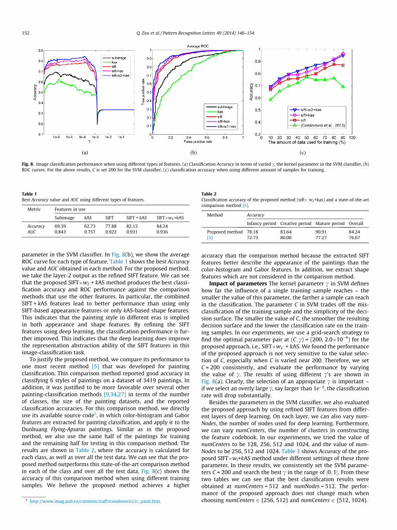
Table 2Classification accuracy of the proposed method (sift� w2+kas) and a state-of-the-artcomparison method [5].

Method Accuracy

Infancy period Creative period Mature period Overall

Proposed method 78.18 83.64 90.91 84.24[5] 72.73 80.00 77.27 76.67

Table 1Best Accuracy value and AUC using different types of features.

Metric Features in use

Subimage kAS SIFT SIFT + kAS SIFT�w2+kAS

Accuracy 69.39 62.73 77.88 82.12 84.24AUC 0.843 0.757 0.922 0.931 0.936

Fig. 8. Image classification performance when using different types of features. (a) Classification Accuracy in terms of varied c, the kernel parameter in the SVM classifier, (b)ROC curves. For the above results, C is set 200 for the SVM classifier, (c) classification accuracy when using different amount of samples for training.

152 Q. Zou et al. / Pattern Recognition Letters 49 (2014) 146–154

parameter in the SVM classifier. In Fig. 8(b), we show the averageROC curve for each type of feature. Table 1 shows the best Accuracyvalue and AUC obtained in each method. For the proposed method,we take the layer-2 output as the refined SIFT feature. We can seethat the proposed SIFT�w2 + kAS method produces the best classi-fication accuracy and ROC performance against the comparisonmethods that use the other features. In particular, the combinedSIFT + kAS features lead to better performance than using onlySIFT-based appearance features or only kAS-based shape features.This indicates that the painting style in different eras is impliedin both appearance and shape features. By refining the SIFTfeatures using deep learning, the classification performance is fur-ther improved. This indicates that the deep learning does improvethe representation abstraction ability of the SIFT features in thisimage-classification task.

To justify the proposed method, we compare its performance toone most recent method [5] that was developed for paintingclassification. This comparison method reported good accuracy inclassifying 6 styles of paintings on a dataset of 3419 paintings. Inaddition, it was justified to be more favorable over several otherpainting-classification methods [9,34,27] in terms of the numberof classes, the size of the painting datasets, and the reportedclassification accuracies. For this comparison method, we directlyuse its available source code5, in which color-histogram and Gaborfeatures are extracted for painting classification, and apply it to theDunhuang Flying-Apsaras paintings. Similar as in the proposedmethod, we also use the same half of the paintings for trainingand the remaining half for testing in this comparison method. Theresults are shown in Table 2, where the accuracy is calculated foreach class, as well as over all the test data. We can see that the pro-posed method outperforms this state-of-the-art comparison methodin each of the class and over all the test data. Fig. 8(c) shows theaccuracy of this comparison method when using different trainingsamples. We believe the proposed method achieves a higher

5 http://www.imag.pub.ro/common/staff/rcondorovici/rc_paint.htm.

accuracy than the comparison method because the extracted SIFTfeatures better describe the appearance of the paintings than thecolor-histogram and Gabor features. In addition, we extract shapefeatures which are not considered in the comparison method.

Impact of parameters The kernel parameter c in SVM defineshow far the influence of a single training sample reaches – thesmaller the value of this parameter, the farther a sample can reachin the classification. The parameter C in SVM trades off the mis-classification of the training sample and the simplicity of the deci-sion surface. The smaller the value of C, the smoother the resultingdecision surface and the lower the classification rate on the train-ing samples. In our experiments, we use a grid-search strategy tofind the optimal parameter pair at (C; c) = (200, 2.0�10�4) for theproposed approach, i.e., SIFT�w2 + kAS. We found the performanceof the proposed approach is not very sensitive to the value selec-tion of C, especially when C is varied near 200. Therefore, we setC = 200 consistently, and evaluate the performance by varyingthe value of c. The results of using different c’s are shown inFig. 8(a). Clearly, the selection of an appropriate c is important –if we select an overly large c, say larger than 1e�3, the classificationrate will drop substantially.

Besides the parameters in the SVM classifier, we also evaluatedthe proposed approach by using refined SIFT features from differ-ent layers of deep learning. On each layer, we can also vary num-Nodes, the number of nodes used for deep learning. Furthermore,we can vary numCenters, the number of clusters in constructingthe feature codebook. In our experiments, we tried the value ofnumCenters to be 128, 256, 512 and 1024, and the value of num-Nodes to be 256, 512 and 1024. Table 3 shows Accuracy of the pro-posed SIFT�wi+kAS method under different settings of these threeparameter. In these results, we consistently set the SVM parame-ters C = 200 and search the best c in the range of ½0;1�. From thesetwo tables we can see that the best classification results wereobtained at numCenters = 512 and numNodes = 512. The perfor-mance of the proposed approach does not change much whenchoosing numCenters 2 {256, 512} and numCenters 2 {512, 1024}.

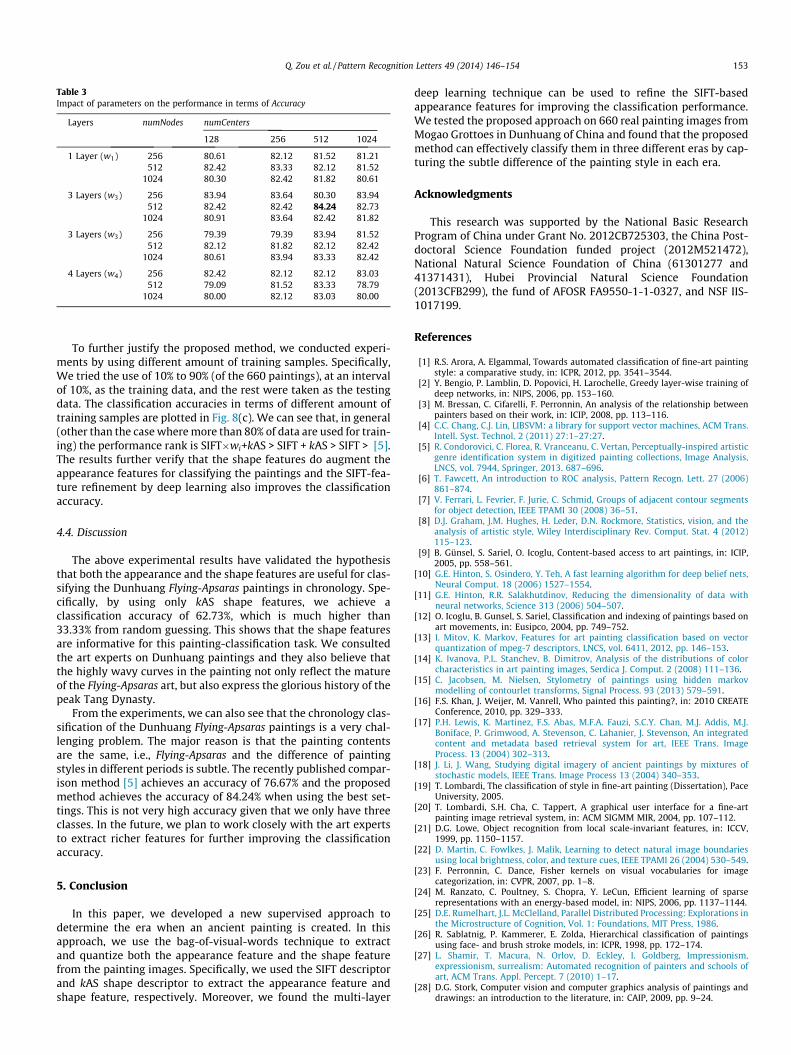
Table 3Impact of parameters on the performance in terms of Accuracy

Layers numNodes numCenters

128 256 512 1024

1 Layer (w1) 256 80.61 82.12 81.52 81.21512 82.42 83.33 82.12 81.52

1024 80.30 82.42 81.82 80.61

3 Layers (w3) 256 83.94 83.64 80.30 83.94512 82.42 82.42 84.24 82.73

1024 80.91 83.64 82.42 81.82

3 Layers (w3) 256 79.39 79.39 83.94 81.52512 82.12 81.82 82.12 82.42

1024 80.61 83.94 83.33 82.42

4 Layers (w4) 256 82.42 82.12 82.12 83.03512 79.09 81.52 83.33 78.79

1024 80.00 82.12 83.03 80.00

Q. Zou et al. / Pattern Recognition Letters 49 (2014) 146–154 153

To further justify the proposed method, we conducted experi-ments by using different amount of training samples. Specifically,We tried the use of 10% to 90% (of the 660 paintings), at an intervalof 10%, as the training data, and the rest were taken as the testingdata. The classification accuracies in terms of different amount oftraining samples are plotted in Fig. 8(c). We can see that, in general(other than the case where more than 80% of data are used for train-ing) the performance rank is SIFT�wi+kAS > SIFT + kAS > SIFT > [5].The results further verify that the shape features do augment theappearance features for classifying the paintings and the SIFT-fea-ture refinement by deep learning also improves the classificationaccuracy.

4.4. Discussion

The above experimental results have validated the hypothesisthat both the appearance and the shape features are useful for clas-sifying the Dunhuang Flying-Apsaras paintings in chronology. Spe-cifically, by using only kAS shape features, we achieve aclassification accuracy of 62.73%, which is much higher than33.33% from random guessing. This shows that the shape featuresare informative for this painting-classification task. We consultedthe art experts on Dunhuang paintings and they also believe thatthe highly wavy curves in the painting not only reflect the matureof the Flying-Apsaras art, but also express the glorious history of thepeak Tang Dynasty.

From the experiments, we can also see that the chronology clas-sification of the Dunhuang Flying-Apsaras paintings is a very chal-lenging problem. The major reason is that the painting contentsare the same, i.e., Flying-Apsaras and the difference of paintingstyles in different periods is subtle. The recently published compar-ison method [5] achieves an accuracy of 76.67% and the proposedmethod achieves the accuracy of 84.24% when using the best set-tings. This is not very high accuracy given that we only have threeclasses. In the future, we plan to work closely with the art expertsto extract richer features for further improving the classificationaccuracy.

5. Conclusion

In this paper, we developed a new supervised approach todetermine the era when an ancient painting is created. In thisapproach, we use the bag-of-visual-words technique to extractand quantize both the appearance feature and the shape featurefrom the painting images. Specifically, we used the SIFT descriptorand kAS shape descriptor to extract the appearance feature andshape feature, respectively. Moreover, we found the multi-layer

deep learning technique can be used to refine the SIFT-basedappearance features for improving the classification performance.We tested the proposed approach on 660 real painting images fromMogao Grottoes in Dunhuang of China and found that the proposedmethod can effectively classify them in three different eras by cap-turing the subtle difference of the painting style in each era.

Acknowledgments

This research was supported by the National Basic ResearchProgram of China under Grant No. 2012CB725303, the China Post-doctoral Science Foundation funded project (2012M521472),National Natural Science Foundation of China (61301277 and41371431), Hubei Provincial Natural Science Foundation(2013CFB299), the fund of AFOSR FA9550-1-1-0327, and NSF IIS-1017199.

References

[1] R.S. Arora, A. Elgammal, Towards automated classification of fine-art paintingstyle: a comparative study, in: ICPR, 2012, pp. 3541–3544.

[2] Y. Bengio, P. Lamblin, D. Popovici, H. Larochelle, Greedy layer-wise training ofdeep networks, in: NIPS, 2006, pp. 153–160.

[3] M. Bressan, C. Cifarelli, F. Perronnin, An analysis of the relationship betweenpainters based on their work, in: ICIP, 2008, pp. 113–116.

[4] C.C. Chang, C.J. Lin, LIBSVM: a library for support vector machines, ACM Trans.Intell. Syst. Technol. 2 (2011) 27:1–27:27.

[5] R. Condorovici, C. Florea, R. Vranceanu, C. Vertan, Perceptually-inspired artisticgenre identification system in digitized painting collections, Image Analysis,LNCS, vol. 7944, Springer, 2013. 687–696.

[6] T. Fawcett, An introduction to ROC analysis, Pattern Recogn. Lett. 27 (2006)861–874.

[7] V. Ferrari, L. Fevrier, F. Jurie, C. Schmid, Groups of adjacent contour segmentsfor object detection, IEEE TPAMI 30 (2008) 36–51.

[8] D.J. Graham, J.M. Hughes, H. Leder, D.N. Rockmore, Statistics, vision, and theanalysis of artistic style, Wiley Interdisciplinary Rev. Comput. Stat. 4 (2012)115–123.

[9] B. Günsel, S. Sariel, O. Icoglu, Content-based access to art paintings, in: ICIP,2005, pp. 558–561.

[10] G.E. Hinton, S. Osindero, Y. Teh, A fast learning algorithm for deep belief nets,Neural Comput. 18 (2006) 1527–1554.

[11] G.E. Hinton, R.R. Salakhutdinov, Reducing the dimensionality of data withneural networks, Science 313 (2006) 504–507.

[12] O. Icoglu, B. Gunsel, S. Sariel, Classification and indexing of paintings based onart movements, in: Eusipco, 2004, pp. 749–752.

[13] I. Mitov, K. Markov, Features for art painting classification based on vectorquantization of mpeg-7 descriptors, LNCS, vol. 6411, 2012, pp. 146–153.

[14] K. Ivanova, P.L. Stanchev, B. Dimitrov, Analysis of the distributions of colorcharacteristics in art painting images, Serdica J. Comput. 2 (2008) 111–136.

[15] C. Jacobsen, M. Nielsen, Stylometry of paintings using hidden markovmodelling of contourlet transforms, Signal Process. 93 (2013) 579–591.

[16] F.S. Khan, J. Weijer, M. Vanrell, Who painted this painting?, in: 2010 CREATEConference, 2010, pp. 329–333.

[17] P.H. Lewis, K. Martinez, F.S. Abas, M.F.A. Fauzi, S.C.Y. Chan, M.J. Addis, M.J.Boniface, P. Grimwood, A. Stevenson, C. Lahanier, J. Stevenson, An integratedcontent and metadata based retrieval system for art, IEEE Trans. ImageProcess. 13 (2004) 302–313.

[18] J. Li, J. Wang, Studying digital imagery of ancient paintings by mixtures ofstochastic models, IEEE Trans. Image Process 13 (2004) 340–353.

[19] T. Lombardi, The classification of style in fine-art painting (Dissertation), PaceUniversity, 2005.

[20] T. Lombardi, S.H. Cha, C. Tappert, A graphical user interface for a fine-artpainting image retrieval system, in: ACM SIGMM MIR, 2004, pp. 107–112.

[21] D.G. Lowe, Object recognition from local scale-invariant features, in: ICCV,1999, pp. 1150–1157.

[22] D. Martin, C. Fowlkes, J. Malik, Learning to detect natural image boundariesusing local brightness, color, and texture cues, IEEE TPAMI 26 (2004) 530–549.

[23] F. Perronnin, C. Dance, Fisher kernels on visual vocabularies for imagecategorization, in: CVPR, 2007, pp. 1–8.

[24] M. Ranzato, C. Poultney, S. Chopra, Y. LeCun, Efficient learning of sparserepresentations with an energy-based model, in: NIPS, 2006, pp. 1137–1144.

[25] D.E. Rumelhart, J.L. McClelland, Parallel Distributed Processing: Explorations inthe Microstructure of Cognition, Vol. 1: Foundations, MIT Press, 1986.

[26] R. Sablatnig, P. Kammerer, E. Zolda, Hierarchical classification of paintingsusing face- and brush stroke models, in: ICPR, 1998, pp. 172–174.

[27] L. Shamir, T. Macura, N. Orlov, D. Eckley, I. Goldberg, Impressionism,expressionism, surrealism: Automated recognition of painters and schools ofart, ACM Trans. Appl. Percept. 7 (2010) 1–17.

[28] D.G. Stork, Computer vision and computer graphics analysis of paintings anddrawings: an introduction to the literature, in: CAIP, 2009, pp. 9–24.

154 Q. Zou et al. / Pattern Recognition Letters 49 (2014) 146–154

[29] B. Temel, N. Kilic, B. Ozgultekin, O.N. Ucan, Separation of original paintings ofmatisse and his fakes using wavelet and artificial neural networks, J. Electr.Electron. Eng. 9 (2009) 791–796.

[30] A. Vedaldi, B. Fulkerson, VLFeat: an open and portable library of computervision algorithms, 2008. <http://www.vlfeat.org/>.

[31] J. Weijer, C. Schmid, J. Verbeek, Learning color names from real-world images,in: CVPR, 2007, pp. 1–8.

[32] X. Yu, L. Yi, C. Fermuller, D. Doermann, Object detection using a shapecodebook, in: BMVC, 2007, pp. 1–10.

[33] S. Zhong, Y. Liu, Y. Liu, Bilinear deep learning for image classification, ACMMultimedia (2011) 343–352.

[34] J. Zujovic, L. Gandy, S. Friedman, B. Pardo, T.N. Pappas, Classifying paintings byartistic genre: an analysis of features & classifiers, in: IEEE Int. Workshop onMultimedia Signal Processing, 2009, pp. 1–5.