DEEP ENSEMBLE BAYESIAN ACTIVE LEARNING: AD-DRESSING THE MODE COLLAPSE ISSUE IN MONTECARLO DROPOUT VIA ENSEMBLES

Remus Pop∗The University of Edinburghremus.p.pop@gmail.com

Patric FulopThe University of Edinburghpatric.fulop@ed.ac.uk

ABSTRACT

In image classification tasks, the ability of deep convolutional neural networks(CNNs) to deal with complex image data has proved to be unrivalled. Deep CNNs,however, require large amounts of labeled training data to reach their full poten-tial. In specialized domains such as healthcare, labeled data can be difficult andexpensive to obtain. One way to alleviate this problem is to rely on active learning,a learning technique that aims to reduce the amount of labelled data needed fora specific task while still delivering satisfactory performance. We propose a newactive learning strategy designed for deep neural networks. This method improvesupon the current state-of-the-art deep Bayesian active learning method, which suf-fers from the mode collapse problem. We correct for this deficiency by makinguse of the expressive power and statistical properties of model ensembles. Ourproposed method manages to capture superior data uncertainty, which translatesinto improved classification performance. We demonstrate empirically that ourensemble method yields faster convergence of CNNs trained on the MNIST andCIFAR-10 datasets.

1 INTRODUCTION

The success of deep learning in the last decade has been attributed to more computational power,better algorithms and larger datasets. In object classification tasks, CNNs widely outperform alter-native methods in benchmark datasets (LeCun et al., 2015) and have been used in medical imagingfor critical situations such as skin cancer detection (Haenssle et al., 2018), retinal disease detection(De Fauw et al., 2018) or even brain tumour survival prediction (Lao et al., 2017).

Although their performance is unrivalled, their success strongly depends on huge amounts of anno-tated data (Bengio et al., 2007; Krizhevsky et al., 2012). In specialized domains such as medicineor chemistry, expert labelled data is costly and time consuming to acquire (Hoi et al., 2006; Smithet al., 2018). Active Learning (AL) provides a theoretically sound framework (Cohn et al., 1996)that reduces the amount of labelled data needed for a specific task. Developed as an iterative pro-cess, AL progressively adds unlabelled data points to the training set using an acquisition function,ranking them in order of importance to maximize performance.

Using Active Learning within a Deep Learning framework (DAL) has recently seen successful ap-plications in text classification (Zhang et al., 2017; Shen et al., 2017), visual question answering(Lin & Parikh, 2017) and image classification with CNNs (Gal et al., 2017; Sener & Savarese, 2017;Beluch et al., 2018). One key difference between DAL and classical AL is the sampling in batches,which is needed to keep computational costs low. As such, developing scalable DAL methods forCNNs presents challenging problems. Firstly, acquisitions functions do not scale well for high di-mensional data or parameter spaces, due to the cost of estimating uncertainty measures, which isthe main approach. Secondly, even with scalability not being an issue, one needs to obtain gooduncertainty estimates in order to avoid having overconfident predictions. One of the most promisingtechniques is Deep Bayesian Active Learning (DBAL) (Gal, 2016; Gal & Ghahramani, 2016), whichuses Monte-Carlo dropout (MC-dropout) as a Bayesian framework to obtain uncertainty estimates.

∗This work was developed as part of the master thesis requirements at The University of Edinburgh

1

arX

iv:1

811.

0389

7v1

[cs

.LG

] 9

Nov

201

8

However, as mentioned in Ducoffe & Precioso (2018), uncertainty-based methods can be fooled byadversarial examples, where small perturbations in inputs can result in overconfident and surprisingoutputs. Another approach presented by Beluch et al. (2018) uses ensemble models to obtain betteruncertainty estimates than DBAL methods, although there are no result on how it deals with adver-sarial perturbations. Whereas uncertainty-based methods aim to pick data points the model is mostuncertain about, density-based approaches try to identify the samples that are most representativeof the entire unlabelled set, albeit at a computational cost (Sener & Savarese, 2017). Hybrid meth-ods aim to trade uncertainty for representativeness. Our belief is that overconfident predictions forDBAL methods are an outcome of the mode collapse phenomenon in variational inference methods(Srivastava et al., 2017), and that by combining the expressive power of ensemble methods withMC-dropout we can obtain ”better” uncertainties without trading representativeness.

In this paper we provide evidence for the mode collapse phenomenon in the form of a highly im-balanced training set acquired during AL with MC-dropout, and show that ’preferential’ behaviouris not beneficial for the AL process. Furthermore, we link the mode collapse phenomenon to over-confident classifications. We compare the use of ensemble models to MC-Dropout for uncertaintyestimation and give intuitive reasons why combining the two might perform better. We presentDeep Ensemble Bayesian Active Learning (DEBAL) which confirms our intuition for experimentson MNIST and CIFAR-10.

In Section 2 we give an overview of current popular methods for DAL. In Section 3, various acqui-sition functions are introduced and the mode collapse issue is empirically identified. Further on, theuse of model ensembles is motivated before presenting our method DEBAL. The last part of section3 is devoted to understanding the cause of the observed improvements in performance.

2 BACKGROUND

The area of active learning has been studied extensively before (see Settles (2012) for a comprehen-sive review), but with the emergence of deep learning, it has seen widespread interest. As provedby Dasgupta (2005) there is no good universal AL strategy, researchers instead relying on heuristicstailored for their particular tasks.

Uncertainty-based Methods. We identify uncertainty-based methods as being the main ones usedby the image classification community. Deep Bayesian Active Learning (Gal et al., 2017) mod-els a Gaussian prior over the CNNs weights and uses variational inference techniques to obtain aposterior distribution over the network’s predictions, using these samples as a measure of uncer-tainty and as input to the acquisition function of the AL process. In practice, posterior samples areobtained using Monte-Carlo dropout (MC-dropout)(Srivastava et al., 2014), a computationally inex-pensive and powerful stochastic regularization technique that performs well on real-world datasets(Leibig et al., 2017; Kendall et al., 2015) and has been shown to be equivalent to performing vari-ational inference (Gal & Ghahramani, 2016). However, these approximating methods suffer frommode collapse, as evidenced in Blei et al. (2017). Another method, Cost-Effective Active Learning(CEAL) (Wang et al., 2016), uses the entropy of the network’s outputs to quantify uncertainty, withadditional pseudo-labelling. This can be seen as the deterministic counterpart of DBAL, that addshighly confident samples directly from predictions, without the query process. Kading et al. (2016)propose a method on the expected model output change principle. This method approximates the ex-pected reduction in the model’s error to avoid selecting redundant queries, albeit at a computationalcost. Lastly, as this work was being developed, we found the work of Beluch et al. (2018), whopropose to use deterministic ensemble models to obtain uncertainty approximations. Their methodscores high both in terms of performance and robustness.

Density-based Methods & Hybrid Methods. Sener & Savarese (2017) looked at the data selectionprocess from a set theory approach (core set) and showed their heuristic-free method outperformsexisting uncertainty-based ones. Their acquisition function uses the geometry in the data-space toselect the most informative samples. The main idea is to try to find a diverse subset of the en-tire input data space that best represents it. Although achieving promising results, the core setapproach is computationally expensive as it requires solving a mixed integer programming optimi-sation problem. Ducoffe & Precioso (2018), on the other hand, rely on adversarial perturbation toselect unlabeled samples. Their approach can be seen as margin based active learning, wherebydistances to decision boundaries are approximated by distances to adversarial examples. To the best

2

of our knowledge, the only hybrid method (combining measures of both uncertainty and represen-tativeness) tested within a CNN-based DAL framework is the one proposed in Wang & Ye (2015).Although originally not tested on CNNs, this method was shown to perform worse than the core setapproach in Sener & Savarese (2017).

Deep Bayesian Active Learning. Given the set of inputs X = {x1, ..,xn} and outputs Y ={y1, .., yn} belonging to classes c, one can define a probabilistic neural network by defining a modelf(x;θ) with a prior p(θ) over the parameter space θ, usually Gaussian, and a likelihood p(y =c|x,θ) which is usually given by softmax(f(x;θ)). The goal is to obtain the posterior distributionover θ:

p(θ|X,Y) = p(Y|X,θ)p(θ)p(Y|X)

(1)

One can make predictions y∗ about new data points x∗ by taking a weighted average of the forecastsobtained using all possible values of the parameters θ, weighted by the posterior probability of eachparameter:

p(y∗|x∗,X,Y) =∫

p(y∗|x,θ)p(θ|X,Y)dθ = Eθ∼p(θ|X,Y)[f(x;θ)] (2)

The real difficulty arises when trying to compute these expectations, as has been previously coveredin the literature (Neal, 2012; Hinton & Van Camp, 1993; Barber & Bishop, 1998; Lawrence, 2001).One way to circumvent this issue is to use Monte Carlo (MC) techniques (Hoffman et al., 2013;Paisley et al., 2012; Kingma & Welling, 2013), which approximate the exact expectations using av-erages over finite independent samples from the posterior predictive distribution (Robert & Casella,2013). The MC-Dropout technique (Srivastava et al., 2014) will replace p(θ|X,Y) with the dropoutdistribution q(θ). This method scales well to high dimensional data, it is highly flexible to accom-modate complex models and it is extremely applicable to existing neural network architectures, aswell as easy to use.

In DBAL (Gal, 2016), the authors incorporate Bayesian uncertainty via MC-dropout and use acqui-sition functions that originate from information theory to try and capture two types of uncertainty:epistemic and aleatoric (Smith & Gal, 2018; Depeweg et al., 2017). Epistemic uncertainty is aconsequence of insufficient learning of model parameters due to lack of data, leading to broad pos-teriors. On the other hand, aleatoric uncertainty arises due to the genuine stochasticity in the data(noise) and always leads to predictions with high uncertainty. We briefly describe the three maintypes of acquisition functions:

• MaxEntropy (Shannon, 2001). The higher the entropy of the predictive distribution, themore uncertain the model is:

H[y|x,θ] = −∑c

p(y = c|x,θ)logp(y = c|x,θ) (3)

• Bayesian Active Learning by Disagreement (BALD) (Houlsby et al., 2011). Based on themutual information between the input data and posterior, and quantifies the informationgain about the model parameters if the correct label would be provided.

I(y,θ|x,θ) = H[y|x;X,Y]− Eθ∼p(θ|X,Y)

[H[y|x,θ]

](4)

• Variation Ratio (Freeman, 1965). Measures the statistical dispersion of a categorical vari-able, with larger values indicating higher uncertainty:

VarRatio(x) = 1−maxy

p(y|x,θ) (5)

As seen in Gal (2016), for the above deterministic acquisition functions we can write the stochas-tic versions using the Bayesian MC-Dropout framework, where the class conditional probabilityp(y|x,θ) can be approximated by the average over the MC-Dropout forward passes. The stochasticpredictive entropy becomes:

H[y|x,θ] = −∑c

( 1

K

∑k

p(y = c|x,θk))log( 1

K

∑k

p(y = c|x,θk))

(6)

K corresponds to the total number of MC-Dropout forward passes at test time. Equivalent stochasticversions can be obtained for all other acquisition functions.

3

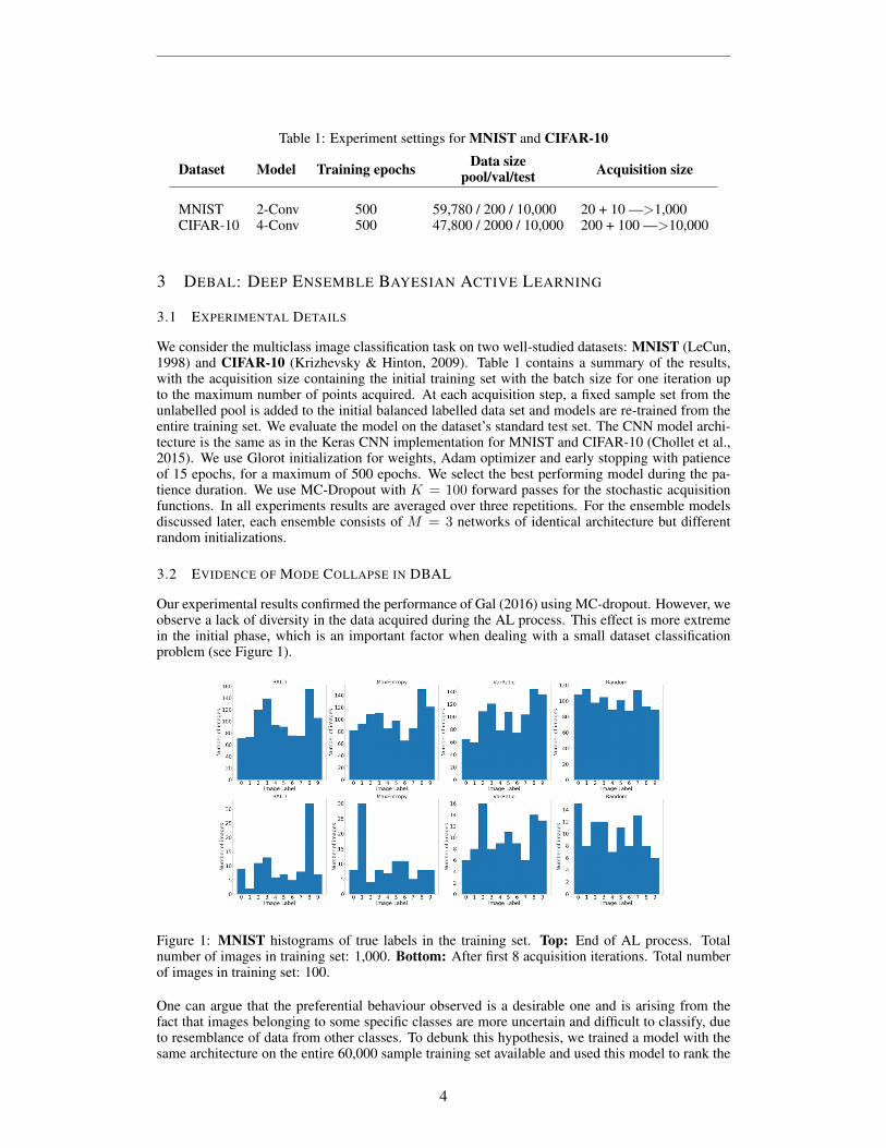
Table 1: Experiment settings for MNIST and CIFAR-10

Dataset Model Training epochs Data sizepool/val/test Acquisition size

MNIST 2-Conv 500 59,780 / 200 / 10,000 20 + 10 —>1,000CIFAR-10 4-Conv 500 47,800 / 2000 / 10,000 200 + 100 —>10,000

3 DEBAL: DEEP ENSEMBLE BAYESIAN ACTIVE LEARNING

3.1 EXPERIMENTAL DETAILS

We consider the multiclass image classification task on two well-studied datasets: MNIST (LeCun,1998) and CIFAR-10 (Krizhevsky & Hinton, 2009). Table 1 contains a summary of the results,with the acquisition size containing the initial training set with the batch size for one iteration upto the maximum number of points acquired. At each acquisition step, a fixed sample set from theunlabelled pool is added to the initial balanced labelled data set and models are re-trained from theentire training set. We evaluate the model on the dataset’s standard test set. The CNN model archi-tecture is the same as in the Keras CNN implementation for MNIST and CIFAR-10 (Chollet et al.,2015). We use Glorot initialization for weights, Adam optimizer and early stopping with patienceof 15 epochs, for a maximum of 500 epochs. We select the best performing model during the pa-tience duration. We use MC-Dropout with K = 100 forward passes for the stochastic acquisitionfunctions. In all experiments results are averaged over three repetitions. For the ensemble modelsdiscussed later, each ensemble consists of M = 3 networks of identical architecture but differentrandom initializations.

3.2 EVIDENCE OF MODE COLLAPSE IN DBAL

Our experimental results confirmed the performance of Gal (2016) using MC-dropout. However, weobserve a lack of diversity in the data acquired during the AL process. This effect is more extremein the initial phase, which is an important factor when dealing with a small dataset classificationproblem (see Figure 1).

Figure 1: MNIST histograms of true labels in the training set. Top: End of AL process. Totalnumber of images in training set: 1,000. Bottom: After first 8 acquisition iterations. Total numberof images in training set: 100.

One can argue that the preferential behaviour observed is a desirable one and is arising from thefact that images belonging to some specific classes are more uncertain and difficult to classify, dueto resemblance of data from other classes. To debunk this hypothesis, we trained a model with thesame architecture on the entire 60,000 sample training set available and used this model to rank the

4

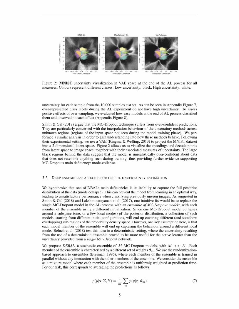
Figure 2: MNIST uncertainty visualization in VAE space at the end of the AL process for allmeasures. Colours represent different classes. Low uncertainty: black, High uncertainty: white.

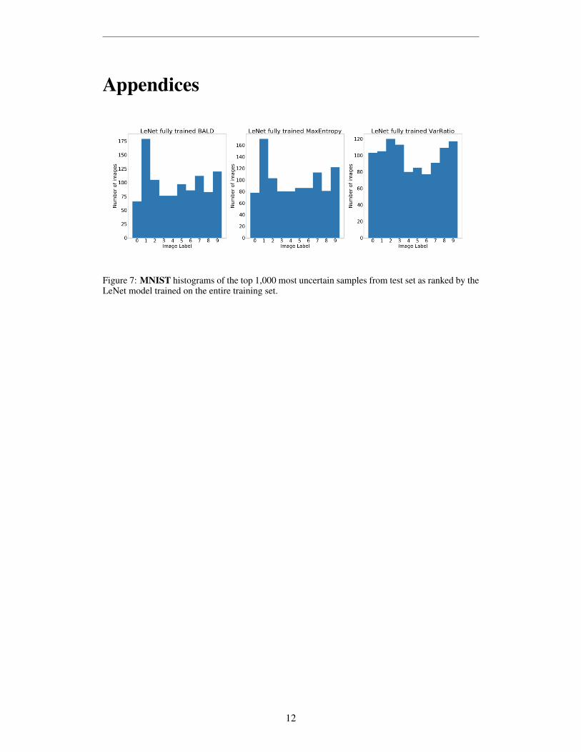
uncertainty for each sample from the 10,000 samples test set. As can be seen in Appendix Figure 7,over-represented class labels during the AL experiment do not have high uncertainty. To assesspositive effects of over-sampling, we evaluated how easy models at the end of AL process classifiedthem and observed no such effect (Appendix Figure 8).

Smith & Gal (2018) argue that the MC-Dropout technique suffers from over-confident predictions.They are particularly concerned with the interpolation behaviour of the uncertainty methods acrossunknown regions (regions of the input space not seen during the model training phase). We per-formed a similar analysis in order to gain understanding into how these methods behave. Followingtheir experimental setting, we use a VAE (Kingma & Welling, 2013) to project the MNIST datasetinto a 2-dimensional latent space. Figure 2 allows us to visualize the encodings and decode pointsfrom latent space to image space, together with their associated measures of uncertainty. The largeblack regions behind the data suggest that the model is unrealistically over-confident about datathat does not resemble anything seen during training, thus providing further evidence supportingMC-Dropouts main deficiency: mode-collapse.

3.3 DEEP ENSEMBLES: A RECIPE FOR USEFUL UNCERTAINTY ESTIMATION

We hypothesize that one of DBALs main deficiencies is its inability to capture the full posteriordistribution of the data (mode collapse). This can prevent the model from learning in an optimal way,leading to unsatisfactory performance when classifying previously unseen images. As suggested inSmith & Gal (2018) and Lakshminarayanan et al. (2017), one intuitive fix would be to replace thesingle MC-Dropout model in the AL process with an ensemble of MC-Dropout models, with eachmember of the ensemble using a different initialization. Since one MC-Dropout model collapsesaround a subspace (one, or a few local modes) of the posterior distribution, a collection of suchmodels, starting from different initial configurations, will end up covering different (and somehowoverlapping) sub-regions of the probability density space. However, one key assumption here, is thateach model member of the ensemble will end up capturing the behaviour around a different localmode. Beluch et al. (2018) test this idea in a deterministic setting, where the uncertainty resultingfrom the use of a deterministic ensemble proved to be more useful for the active learner than theuncertainty provided from a single MC-Dropout network.

We propose DEBAL, a stochastic ensemble of M MC-Dropout models, with M << K. Eachmember of the ensemble is characterized by a different set of weights θm. We use the randomization-based approach to ensembles (Breiman, 1996), where each member of the ensemble is trained inparallel without any interaction with the other members of the ensemble. We consider the ensembleas a mixture model where each member of the ensemble is uniformly weighted at prediction time.For our task, this corresponds to averaging the predictions as follows:

p(y|x;X,Y) = 1

M

∑m

p(y|x,θm) (7)

5

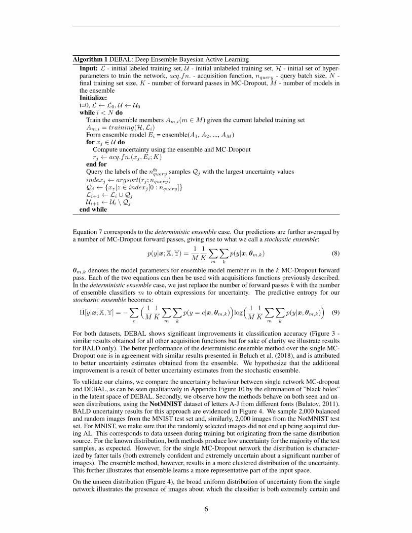
Algorithm 1 DEBAL: Deep Ensemble Bayesian Active LearningInput: L - initial labeled training set, U - initial unlabeled training set, H - initial set of hyper-parameters to train the network, acq.fn. - acquisition function, nquery - query batch size, N -final training set size, K - number of forward passes in MC-Dropout, M - number of models inthe ensembleInitialize:i=0, L ← L0, U ← U0while i < N do

Train the ensemble members Am,i(m ∈M ) given the current labeled training setAm,i = training(H,Li)Form ensemble model Ei = ensemble(A1, A2, ..., AM )for xj ∈ U do

Compute uncertainty using the ensemble and MC-Dropoutrj ← acq.fn.(xj , Ei;K)

end forQuery the labels of the nth

query samples Qj with the largest uncertainty valuesindexj ← argsort(rj ;nquery)Qj ← {xz|z ∈ indexj [0 : nquery]}Li+1 ← Li ∪Qj

Ui+1 ← Ui \ Qj

end while

Equation 7 corresponds to the deterministic ensemble case. Our predictions are further averaged bya number of MC-Dropout forward passes, giving rise to what we call a stochastic ensemble:

p(y|x;X,Y) = 1

M

1

K

∑m

∑k

p(y|x,θm,k) (8)

θm,k denotes the model parameters for ensemble model member m in the k MC-Dropout forwardpass. Each of the two equations can then be used with acquisitions functions previously described.In the deterministic ensemble case, we just replace the number of forward passes k with the numberof ensemble classifiers m to obtain expressions for uncertainty. The predictive entropy for ourstochastic ensemble becomes:

H[y|x;X,Y] = −∑c

( 1

M

1

K

∑m

∑k

p(y = c|x,θm,k))log( 1

M

1

K

∑m

∑k

p(y|x,θm,k))

(9)

For both datasets, DEBAL shows significant improvements in classification accuracy (Figure 3 -similar results obtained for all other acquisition functions but for sake of clarity we illustrate resultsfor BALD only). The better performance of the deterministic ensemble method over the single MC-Dropout one is in agreement with similar results presented in Beluch et al. (2018), and is attributedto better uncertainty estimates obtained from the ensemble. We hypothesize that the additionalimprovement is a result of better uncertainty estimates from the stochastic ensemble.

To validate our claims, we compare the uncertainty behaviour between single network MC-dropoutand DEBAL, as can be seen qualitatively in Appendix Figure 10 by the elimination of ”black holes”in the latent space of DEBAL. Secondly, we observe how the methods behave on both seen and un-seen distributions, using the NotMNIST dataset of letters A-J from different fonts (Bulatov, 2011).BALD uncertainty results for this approach are evidenced in Figure 4. We sample 2,000 balancedand random images from the MNIST test set and, similarly, 2,000 images from the NotMNIST testset. For MNIST, we make sure that the randomly selected images did not end up being acquired dur-ing AL. This corresponds to data unseen during training but originating from the same distributionsource. For the known distribution, both methods produce low uncertainty for the majority of the testsamples, as expected. However, for the single MC-Dropout network the distribution is character-ized by fatter tails (both extremely confident and extremely uncertain about a significant number ofimages). The ensemble method, however, results in a more clustered distribution of the uncertainty.This further illustrates that ensemble learns a more representative part of the input space.

On the unseen distribution (Figure 4), the broad uniform distribution of uncertainty from the singlenetwork illustrates the presence of images about which the classifier is both extremely certain and

6

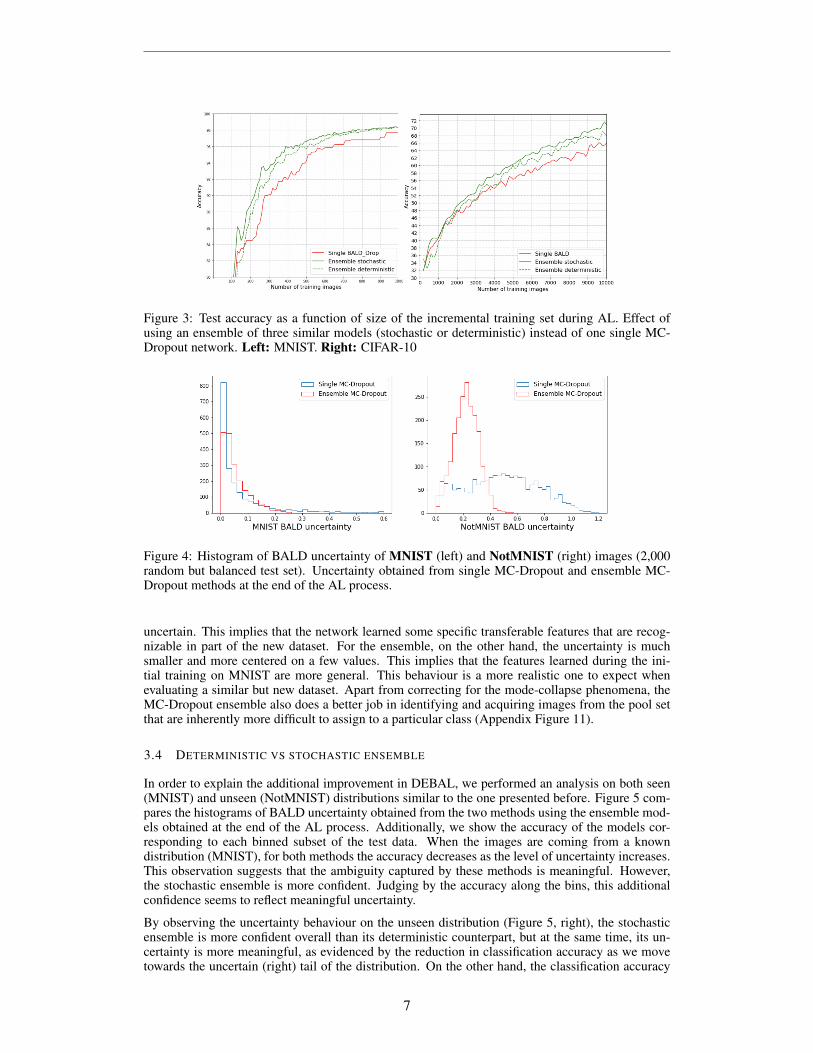
Figure 3: Test accuracy as a function of size of the incremental training set during AL. Effect ofusing an ensemble of three similar models (stochastic or deterministic) instead of one single MC-Dropout network. Left: MNIST. Right: CIFAR-10

Figure 4: Histogram of BALD uncertainty of MNIST (left) and NotMNIST (right) images (2,000random but balanced test set). Uncertainty obtained from single MC-Dropout and ensemble MC-Dropout methods at the end of the AL process.

uncertain. This implies that the network learned some specific transferable features that are recog-nizable in part of the new dataset. For the ensemble, on the other hand, the uncertainty is muchsmaller and more centered on a few values. This implies that the features learned during the ini-tial training on MNIST are more general. This behaviour is a more realistic one to expect whenevaluating a similar but new dataset. Apart from correcting for the mode-collapse phenomena, theMC-Dropout ensemble also does a better job in identifying and acquiring images from the pool setthat are inherently more difficult to assign to a particular class (Appendix Figure 11).

3.4 DETERMINISTIC VS STOCHASTIC ENSEMBLE

In order to explain the additional improvement in DEBAL, we performed an analysis on both seen(MNIST) and unseen (NotMNIST) distributions similar to the one presented before. Figure 5 com-pares the histograms of BALD uncertainty obtained from the two methods using the ensemble mod-els obtained at the end of the AL process. Additionally, we show the accuracy of the models cor-responding to each binned subset of the test data. When the images are coming from a knowndistribution (MNIST), for both methods the accuracy decreases as the level of uncertainty increases.This observation suggests that the ambiguity captured by these methods is meaningful. However,the stochastic ensemble is more confident. Judging by the accuracy along the bins, this additionalconfidence seems to reflect meaningful uncertainty.

By observing the uncertainty behaviour on the unseen distribution (Figure 5, right), the stochasticensemble is more confident overall than its deterministic counterpart, but at the same time, its un-certainty is more meaningful, as evidenced by the reduction in classification accuracy as we movetowards the uncertain (right) tail of the distribution. On the other hand, the classification accuracy

7

Figure 5: Histogram of BALD uncertainty of MNIST (left) and NotMNIST (right) images (2,000random but balanced test set). Uncertainty obtained from deterministic and MC-Dropout ensemblemethods at the end of the AL process. Numbers correspond to accuracy for corresponding binnedsubset of test data (in percentage).

Figure 6: Left MNIST uncertainty calibration. Expected fraction and observed fraction. Ideal outputis the dashed black line. MSE reported in paranthesis. Calibration averaged over 3 different runs.

of the deterministic ensemble is more uniform, with both tails of the distributions (most and leastcertain) seeing similar levels of accuracy. This suggests that the uncertainty produced by the deter-ministic ensemble is less correlated with the level of its uncertainty and hence less meaningful.

Uncertainty calibration. We used the ensemble models obtained at the end of the AL experimentsto evaluate the entire MNIST test set. We looked whether the expected fraction of correct classifica-tions matches the observed proportion. The expected proportion of correct classifications is derivedfrom the models confidence. When plotting expected against observed fraction, a well-calibratedmodel should lie very close to the diagonal. Figure 6(left) shows that the stochastic ensemble methodleads to a better calibrated uncertainty. An additional measure for uncertainty calibration (quality) isthe Brier score (Brier, 1950), where a smaller value corresponds to better calibrated predictions. Wefind that the stochastic ensemble has a better quality of uncertainty (Brier score: 0.0244) comparedto the deterministic one (Brier score: 0.0297). Finally, we investigated the effect of training thedeterministic ensemble with data acquired by the stochastic one. Figure 6 (right) shows that incor-porating stochasticity in the ensemble via MC-Dropout leads to an overall increase in performance,further reinforcing our hypothesis.

4 CONCLUSION AND FUTURE WORK

In this work, we focused on the use of active learning in a deep learning framework for the imageclassification task. We showed empirically how the mode collapse phenomenon is having a negativeimpact on the current state-of-the-art Bayesian active learning method. We improved upon thismethod by leveraging off the expressive power and statistical properties of model ensembles. Welinked the performance improvement to a better representation of data uncertainty resulting fromour method. For future work, this superior uncertainty representation could be used to address oneof the major issues of deep networks in safety-critical applications: adversarial examples.

8

REFERENCES

David Barber and Christopher M Bishop. Ensemble learning in bayesian neural networks. NATOASI SERIES F COMPUTER AND SYSTEMS SCIENCES, 168:215–238, 1998.

William H Beluch, Tim Genewein, Andreas Nurnberger, and Jan M Kohler. The power of ensemblesfor active learning in image classification. In Proceedings of the IEEE Conference on ComputerVision and Pattern Recognition, pp. 9368–9377, 2018.

Yoshua Bengio, Pascal Lamblin, Dan Popovici, and Hugo Larochelle. Greedy layer-wise trainingof deep networks. In Advances in neural information processing systems, pp. 153–160, 2007.

David M Blei, Alp Kucukelbir, and Jon D McAuliffe. Variational inference: A review for statisti-cians. Journal of the American Statistical Association, 112(518):859–877, 2017.

Leo Breiman. Bagging predictors. Machine learning, 24(2):123–140, 1996.

Glenn W Brier. Verification of forecasts expressed in terms of probability. Monthey Weather Review,78(1):1–3, 1950.

Yaroslav Bulatov. Notmnist dataset. Google (Books/OCR), Tech. Rep.[Online]. Available:http://yaroslavvb. blogspot. it/2011/09/notmnist-dataset. html, 2011.

Francois Chollet et al. Keras. https://keras.io, 2015.

David A Cohn, Zoubin Ghahramani, and Michael I Jordan. Active learning with statistical models.Journal of artificial intelligence research, 4:129–145, 1996.

Sanjoy Dasgupta. Analysis of a greedy active learning strategy. In Advances in neural informationprocessing systems, pp. 337–344, 2005.

Jeffrey De Fauw, Joseph R Ledsam, Bernardino Romera-Paredes, Stanislav Nikolov, Nenad Toma-sev, Sam Blackwell, Harry Askham, Xavier Glorot, Brendan ODonoghue, Daniel Visentin, et al.Clinically applicable deep learning for diagnosis and referral in retinal disease. Nature medicine,24(9):1342, 2018.

Stefan Depeweg, Jose Miguel Hernandez-Lobato, Finale Doshi-Velez, and Steffen Udluft. Un-certainty decomposition in bayesian neural networks with latent variables. arXiv preprintarXiv:1706.08495, 2017.

Melanie Ducoffe and Frederic Precioso. Adversarial active learning for deep networks: a marginbased approach. arXiv preprint arXiv:1802.09841, 2018.

Linton C Freeman. Elementary applied statistics: for students in behavioral science. John Wiley &Sons, 1965.

Yarin Gal. Uncertainty in deep learning. University of Cambridge, 2016.

Yarin Gal and Zoubin Ghahramani. Dropout as a bayesian approximation: Representing modeluncertainty in deep learning. In international conference on machine learning, pp. 1050–1059,2016.

Yarin Gal, Riashat Islam, and Zoubin Ghahramani. Deep bayesian active learning with image data.arXiv preprint arXiv:1703.02910, 2017.

HA Haenssle, C Fink, R Schneiderbauer, F Toberer, T Buhl, A Blum, A Kalloo, A Hassen,L Thomas, A Enk, et al. Man against machine: diagnostic performance of a deep learningconvolutional neural network for dermoscopic melanoma recognition in comparison to 58 der-matologists. Annals of Oncology, 2018.

Geoffrey E Hinton and Drew Van Camp. Keeping the neural networks simple by minimizing the de-scription length of the weights. In Proceedings of the sixth annual conference on Computationallearning theory, pp. 5–13. ACM, 1993.

9

Matthew D Hoffman, David M Blei, Chong Wang, and John Paisley. Stochastic variational infer-ence. The Journal of Machine Learning Research, 14(1):1303–1347, 2013.

Steven CH Hoi, Rong Jin, Jianke Zhu, and Michael R Lyu. Batch mode active learning and itsapplication to medical image classification. In Proceedings of the 23rd international conferenceon Machine learning, pp. 417–424. ACM, 2006.

Neil Houlsby, Ferenc Huszar, Zoubin Ghahramani, and Mate Lengyel. Bayesian active learning forclassification and preference learning. arXiv preprint arXiv:1112.5745, 2011.

Christoph Kading, Erik Rodner, Alexander Freytag, and Joachim Denzler. Active and continu-ous exploration with deep neural networks and expected model output changes. arXiv preprintarXiv:1612.06129, 2016.

Alex Kendall, Vijay Badrinarayanan, and Roberto Cipolla. Bayesian segnet: Model uncertaintyin deep convolutional encoder-decoder architectures for scene understanding. arXiv preprintarXiv:1511.02680, 2015.

Diederik P Kingma and Max Welling. Auto-encoding variational bayes. arXiv preprintarXiv:1312.6114, 2013.

Alex Krizhevsky and Geoffrey Hinton. Learning multiple layers of features from tiny images. Tech-nical report, Citeseer, 2009.

Alex Krizhevsky, Ilya Sutskever, and Geoffrey E Hinton. Imagenet classification with deep convo-lutional neural networks. In Advances in neural information processing systems, pp. 1097–1105,2012.

Balaji Lakshminarayanan, Alexander Pritzel, and Charles Blundell. Simple and scalable predictiveuncertainty estimation using deep ensembles. In Advances in Neural Information ProcessingSystems, pp. 6402–6413, 2017.

Jiangwei Lao, Yinsheng Chen, Zhi-Cheng Li, Qihua Li, Ji Zhang, Jing Liu, and Guangtao Zhai.A deep learning-based radiomics model for prediction of survival in glioblastoma multiforme.Scientific reports, 7(1):10353, 2017.

Neil David Lawrence. Variational inference in probabilistic models. PhD thesis, University ofCambridge, 2001.

Yann LeCun. The mnist database of handwritten digits. http://yann. lecun. com/exdb/mnist/, 1998.

Yann LeCun, Yoshua Bengio, and Geoffrey Hinton. Deep learning. Nature, 521(7553):436–444,2015.

Christian Leibig, Vaneeda Allken, Murat Seckin Ayhan, Philipp Berens, and Siegfried Wahl. Lever-aging uncertainty information from deep neural networks for disease detection. Scientific reports,7(1):17816, 2017.

Xiao Lin and Devi Parikh. Active learning for visual question answering: An empirical study. arXivpreprint arXiv:1711.01732, 2017.

Radford M Neal. Bayesian learning for neural networks, volume 118. Springer Science & BusinessMedia, 2012.

John Paisley, David Blei, and Michael Jordan. Variational bayesian inference with stochastic search.arXiv preprint arXiv:1206.6430, 2012.

Christian Robert and George Casella. Monte Carlo statistical methods. Springer Science & BusinessMedia, 2013.

Ozan Sener and Silvio Savarese. Active learning for convolutional neural networks: Acore-setapproach. stat, 1050:27, 2017.

10

Burr Settles. Active learning. Synthesis Lectures on Artificial Intelligence and Machine Learning, 6(1):1–114, 2012.

Claude Elwood Shannon. A mathematical theory of communication. ACM SIGMOBILE mobilecomputing and communications review, 5(1):3–55, 2001.

Yanyao Shen, Hyokun Yun, Zachary C Lipton, Yakov Kronrod, and Animashree Anandkumar. Deepactive learning for named entity recognition. arXiv preprint arXiv:1707.05928, 2017.

Justin S Smith, Ben Nebgen, Nicholas Lubbers, Olexandr Isayev, and Adrian E Roitberg. Less ismore: Sampling chemical space with active learning. The Journal of Chemical Physics, 148(24):241733, 2018.

Lewis Smith and Yarin Gal. Understanding measures of uncertainty for adversarial example detec-tion. arXiv preprint arXiv:1803.08533, 2018.

Akash Srivastava, Lazar Valkoz, Chris Russell, Michael U Gutmann, and Charles Sutton. Vee-gan: Reducing mode collapse in gans using implicit variational learning. In Advances in NeuralInformation Processing Systems, pp. 3308–3318, 2017.

Nitish Srivastava, Geoffrey Hinton, Alex Krizhevsky, Ilya Sutskever, and Ruslan Salakhutdinov.Dropout: A simple way to prevent neural networks from overfitting. The Journal of MachineLearning Research, 15(1):1929–1958, 2014.

Keze Wang, Dongyu Zhang, Ya Li, Ruimao Zhang, and Liang Lin. Cost-effective active learningfor deep image classification. IEEE Transactions on Circuits and Systems for Video Technology,2016.

Zheng Wang and Jieping Ye. Querying discriminative and representative samples for batch modeactive learning. ACM Transactions on Knowledge Discovery from Data (TKDD), 9(3):17, 2015.

Ye Zhang, Matthew Lease, and Byron C Wallace. Active discriminative text representation learning.In AAAI, pp. 3386–3392, 2017.

11

Appendices

Figure 7: MNIST histograms of the top 1,000 most uncertain samples from test set as ranked by theLeNet model trained on the entire training set.

12

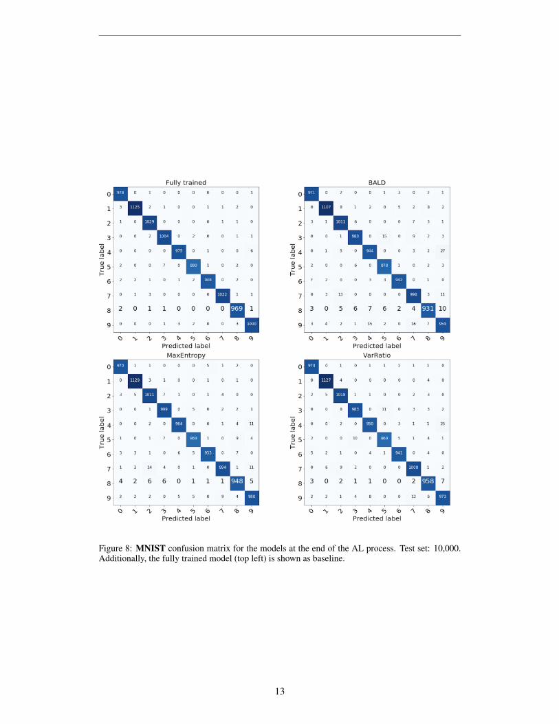
Figure 8: MNIST confusion matrix for the models at the end of the AL process. Test set: 10,000.Additionally, the fully trained model (top left) is shown as baseline.

13

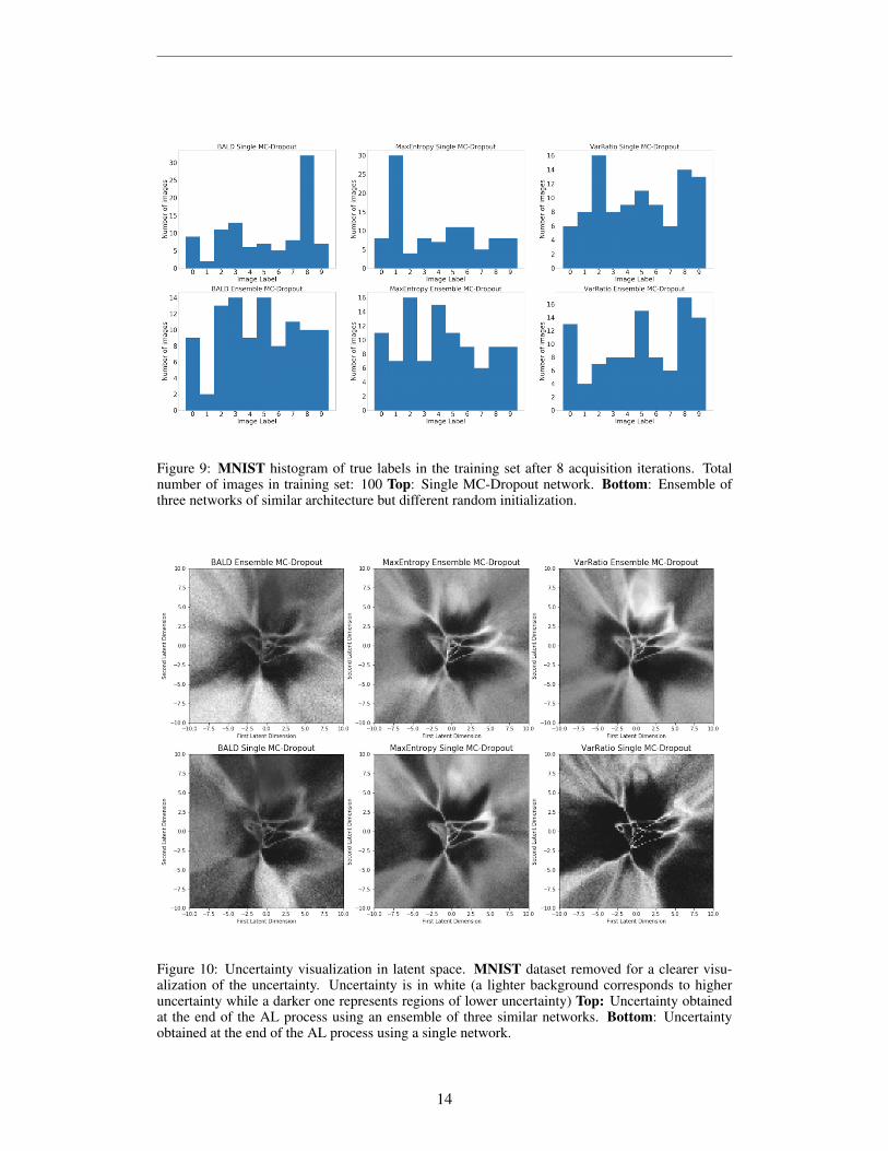
Figure 9: MNIST histogram of true labels in the training set after 8 acquisition iterations. Totalnumber of images in training set: 100 Top: Single MC-Dropout network. Bottom: Ensemble ofthree networks of similar architecture but different random initialization.

Figure 10: Uncertainty visualization in latent space. MNIST dataset removed for a clearer visu-alization of the uncertainty. Uncertainty is in white (a lighter background corresponds to higheruncertainty while a darker one represents regions of lower uncertainty) Top: Uncertainty obtainedat the end of the AL process using an ensemble of three similar networks. Bottom: Uncertaintyobtained at the end of the AL process using a single network.

14

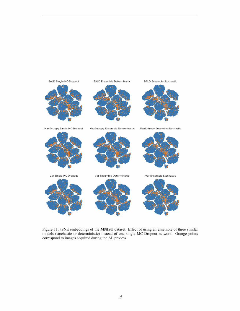
Figure 11: tSNE embeddings of the MNIST dataset. Effect of using an ensemble of three similarmodels (stochastic or deterministic) instead of one single MC-Dropout network. Orange pointscorrespond to images acquired during the AL process.

15