Path, theme and narrativein open plan exhibition settingsdiscovery.ucl.ac.uk/1097/1/PTaN.pdf.pdf ·...

29.1

Proceedings . 4th International Space Syntax Symposium London 2003

29Keywordsmuseum exhibition,spatial layout, path,theme, narrative,learning

[email protected] [email protected]@umich.eduNickDalton <[email protected]>

Path, theme and narrative in open plan exhibition settings

John Peponis1, Ruth Conroy Dalton1, Jean Wineman2, Nick SheepDalton31 Georgia Institute of Technology2 University of Michigan3 Georgia Regional Transportation Authority

AbstractThree arguments are made based on the analysis of science exhibitions. First,sufficiently refined techniques of spatial analysis allow us to model the impact oflayout upon visitors’ paths, even in moderately sized open plans which allow almostrandom patterns of movement and relatively unobstructed visibility. Second, newlydeveloped or adapted techniques of analysis allow us to make a transition frommodeling the mechanics of spatial movement (the way in which movement is affectedby the distribution of obstacles and boundaries), to modeling the manner in whichmovement might register additional aspects of visual information. Third, theadvantages of such purely spatial modes of analysis extend into providing us with asharper understanding of some of the pragmatic constrains within which exhibitioncontent is conceived and designed.

Introducing the question: how do permissive open layouts influence patternsof exhibition exploration?This paper presents new research on the relationship between visitor behavior andlayout in science exhibition settings1. The aims are largely methodological andtheoretical. Previously published studies using techniques similar to the ones thatare used in this study deal with either complex museum environments (Choi, 1999;Turner et al, 2001), or other environments whose spatial structure clearly constrainsand channels movement choices and movement paths in various ways (Conroy-Dalton, 2001). The exhibition settings discussed here are smaller with relativelysimple open plans. Thus, it is intuitively less clear that layout will have significanteffects upon the way in which visitors explore and engage exhibition contents. Thetheoretical and methodological challenge is to examine how exhibition space workswhen it seemingly imposes few non-trivial restrictions upon behavior. In pursuingthis question some fundamental questions about the behavioral and cognitivefunctions of space come into sharper focus.


29.2

The analysis deals with two traveling science exhibitions, each in two differentsettings (Figure 1). Both were created by the same organization, the Carnegie ScienceCenter. “ZAP surgery” presented new technologies for medical operations.“Robotics”, introduced the principles that govern robotic design and function. Thefirst was studied at The Great Lakes Science Center, Cleveland, and at the CarnegieScience Center, Pittsburgh. The second was studied at The Tech museum in SanJose and at the Great Lakes Science Center, Cleveland. All studies were completedin academic year 2000-2001. In both instances, almost all individual exhibits wereinteractive, with the exception of a small number that consisted in video presentationsor in visual information only. Also, individual exhibits were designed to provide aself contained amount of information, but also classified according to conceptualthemes. For example, in the ZAP exhibition displays were visually and spatiallycoordinated according to the following themes: gamma rays, laser beams, cryosurgery,endoscopy and ultra sound. In the case of Robotics, the presentation of displaysreferred to aspects of acting, sensing, areas of application, demonstration of use,and exhibits aimed at “junior” visitors. The conceptual themes were made moreevident visually in the ZAP exhibition, based on the use of color both on individualexhibits and on the background to the corresponding zones of the exhibition. In thecase of Robotics, conceptual themes were less strongly suggested, either by spatialzoning, or through visual design. In both instances, however, the classification ofindividual exhibits by a smaller set of themes was objectively documented in theliterature accompanying the exhibitions, whether in printed catalogues, or in thecorresponding web-pages.

The exhibition settings under study were simple open plans as shown in Figure1. Many individual exhibits, or small groups of individual exhibits were free standing,whether suggesting a peripheral approach, from all sides, or a directional approach,with a clear distinction between front, back and lateral views. Other exhibits arelocated against the perimeter boundary, or against structural elements. The temporary

Figure 1: Diagrammatic plans twoscience exhibitions in different set-tings

29.3


exhibition area itself varied from the relatively compact and clearly bounded shapeof the Great Lakes Science Center, to the more elongated shape of the CarnegieCenter, or the more compact but weakly bounded space at The Tech. The few largeindividual exhibits, such as the ZAP Cam Simulation Capsule in the ZAP exhibition,or the Basketball Robot Arm in the Robotics exhibition, tend to be so located againstthe area boundary as to divide space while at the same time acting as focal points ofvisual attention. There is ample cross visibility between individual exhibits. Thearrangement allows a plethora of alternative exploration paths, as there are relativelyfew impediments to movement. In short, the arrangements under study are not overlydidactic, either in the sense of imposing a deliberate sequence to the pattern ofexploration, or in the sense of framing successive visual fields to control visualgroupings and cross comparisons.

From the point of view of layout, the exhibition settings under study imply amode of discourse where units of knowledge (the units corresponding to individualexhibit elements) are relatively self-contained and where the overall message arisesfrom the quasi-random accumulation of such units. The visitor is left with the taskof re-constructing the exhibition narrative; understanding the layout itself appearsto be no challenge. As used here, the term “narrative” refers to the manner in whichthe contents of individual exhibits can be conceptually related. For example somedisplays suggest that robot design involves the combination of many simple jointssuch that complex movements can result from the combination of simpler motions;other displays suggest that movements of the hand can be translated into mechanicalmovements through simple devices; a third group of displays suggests thatinformation of some sort must be coded and translated in such a way as to causevarious motions; a fourth group suggests that sensors can be used to receiveinformation about changes in the environment. Putting such ideas together, the visitorcan think of robots as mechanisms capable of not only transferring movement butalso of receiving coded instructions for movement, or of processing environmentalinformation in order to produce such instructions. The word “narrative”, therefore,refers to the arrangement of information in logical sequence in a manner that yieldsmore complex insights. In many exhibitions, the sequence in which information isto be received is largely dictated by the layout. In the exhibitions under study, thiswas not the case.

About one hundred visitors were unobtrusively tracked in each setting andtheir paths recorded on diagrammatic plans. When a visitor path came sufficientlyclose to an individual exhibit, such that full awareness of the visual contents of theindividual exhibit was possible, a contact was said to be created. When a visitorstopped at an individual exhibit, whether to physically interact with it or to study its


29.4

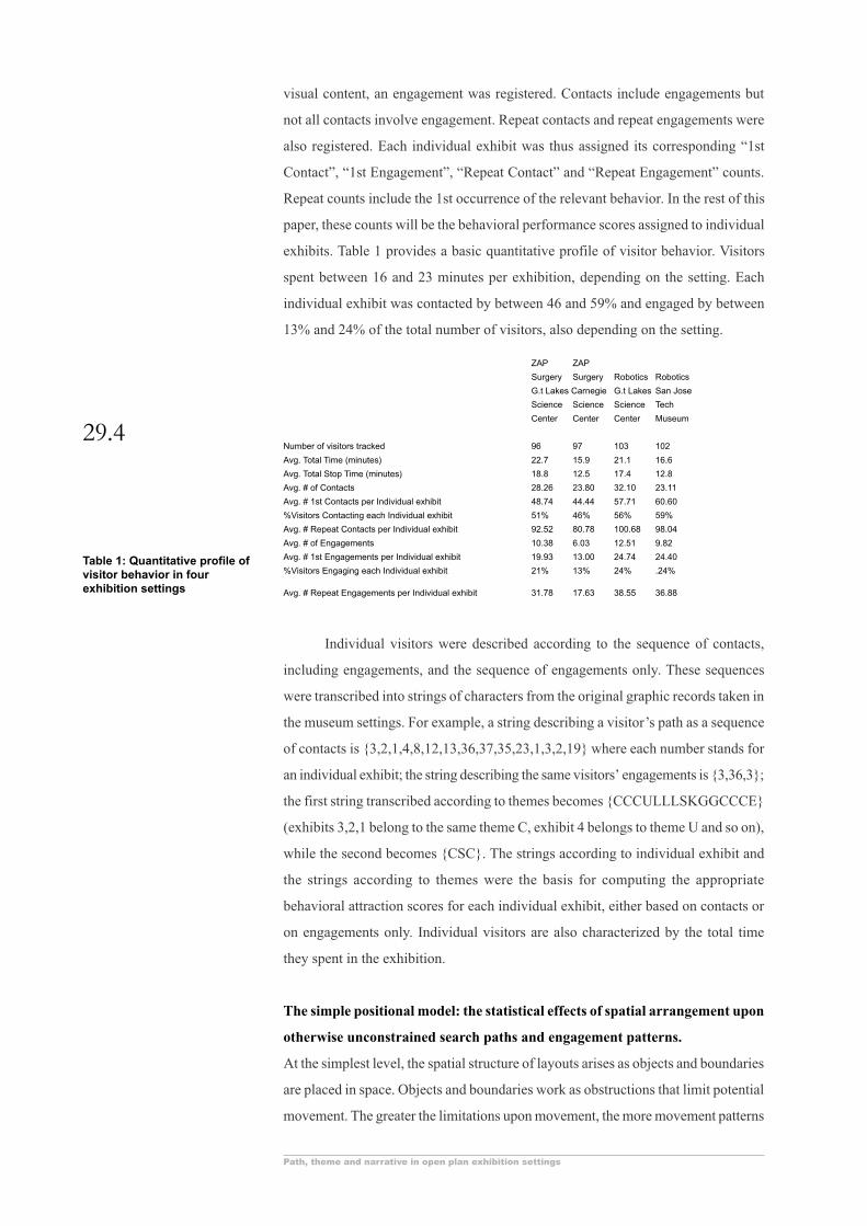
visual content, an engagement was registered. Contacts include engagements butnot all contacts involve engagement. Repeat contacts and repeat engagements werealso registered. Each individual exhibit was thus assigned its corresponding “1stContact”, “1st Engagement”, “Repeat Contact” and “Repeat Engagement” counts.Repeat counts include the 1st occurrence of the relevant behavior. In the rest of thispaper, these counts will be the behavioral performance scores assigned to individualexhibits. Table 1 provides a basic quantitative profile of visitor behavior. Visitorsspent between 16 and 23 minutes per exhibition, depending on the setting. Eachindividual exhibit was contacted by between 46 and 59% and engaged by between13% and 24% of the total number of visitors, also depending on the setting.

ZAP ZAPSurgery Surgery Robotics RoboticsG.t Lakes Carnegie G.t Lakes San JoseScience Science Science TechCenter Center Center Museum

Number of visitors tracked 96 97 103 102Avg. Total Time (minutes) 22.7 15.9 21.1 16.6Avg. Total Stop Time (minutes) 18.8 12.5 17.4 12.8Avg. # of Contacts 28.26 23.80 32.10 23.11Avg. # 1st Contacts per Individual exhibit 48.74 44.44 57.71 60.60%Visitors Contacting each Individual exhibit 51% 46% 56% 59%Avg. # Repeat Contacts per Individual exhibit 92.52 80.78 100.68 98.04Avg. # of Engagements 10.38 6.03 12.51 9.82Avg. # 1st Engagements per Individual exhibit 19.93 13.00 24.74 24.40%Visitors Engaging each Individual exhibit 21% 13% 24% .24%Avg. # Repeat Engagements per Individual exhibit 31.78 17.63 38.55 36.88

Individual visitors were described according to the sequence of contacts,including engagements, and the sequence of engagements only. These sequenceswere transcribed into strings of characters from the original graphic records taken inthe museum settings. For example, a string describing a visitor’s path as a sequenceof contacts is {3,2,1,4,8,12,13,36,37,35,23,1,3,2,19} where each number stands foran individual exhibit; the string describing the same visitors’ engagements is {3,36,3};the first string transcribed according to themes becomes {CCCULLLSKGGCCCE}(exhibits 3,2,1 belong to the same theme C, exhibit 4 belongs to theme U and so on),while the second becomes {CSC}. The strings according to individual exhibit andthe strings according to themes were the basis for computing the appropriatebehavioral attraction scores for each individual exhibit, either based on contacts oron engagements only. Individual visitors are also characterized by the total timethey spent in the exhibition.

The simple positional model: the statistical effects of spatial arrangement uponotherwise unconstrained search paths and engagement patterns.At the simplest level, the spatial structure of layouts arises as objects and boundariesare placed in space. Objects and boundaries work as obstructions that limit potentialmovement. The greater the limitations upon movement, the more movement patterns

Table 1: Quantitative profile ofvisitor behavior in fourexhibition settings

29.5


are distributed according to the layout. Accordingly, the first model developed hereis called “positional” in that spatial structure is considered only according to theeffects of positioning objects and boundaries in space. No attempt is made to recognizethe additional effects of the specific semantic content of individual exhibits. Nor dowe deal with the ways in which individual exhibits may be related across space bysuch characteristics as common coloring, background lighting and so on. However,the fact that each exhibit has a primary face and an associated contact region in itsimmediate spatial neighborhood, where visitors must stand in order to engage it, isacknowledged. The spatial positioning of individual exhibits is described accordingto the properties of the corresponding contact regions. In other words, the positionof exhibits is described according to the properties of the occupiable spaceimmediately in front of them.

Two kinds of layout descriptors are used, those pertaining to the relativeaccessibility of individual exhibits and those pertaining to their cross-visibility.Accessibility was measured based on the analysis of projection polygons. We proposethe term “projection polygon” as an alternative to the more frequently used term“visibility polygon”, or ”isovist” (Benedikt, 1979). A “visibility polygon” or “isovist”encloses all the area that is directly visible 360 degrees from a vantage point. Weprefer the term “projection polygon” to more explicitly recognize the fact that suchpolygons can be drawn not only at eye but also at any other level, such that whatthey describe is the area of space that is geometrically “visible”, or directly connectedto the vantage point, but not necessarily the area visible to a subject at normal eyelevel. In our case, we draw such polygons at foot level, to represent the extent towhich any given position is accessible from other positions (Figure 2). Morespecifically, the Area of a projection polygon measures the amount of space fromwhich the vantage point is directly accessible along an uninterrupted straight line.The indirect accessibility of each position from other positions is described accordingto the pattern of intersection of projection polygons. When two polygons intersect,any point on one that does not lie on their intersection is one direction change awayfrom the vantage point of the other. Accordingly, the directional distance of anypoint of a layout from any other point can be expressed as a function of the minimumnumber of sequentially intersecting projection polygons that must be used to movefrom one position to the other. Consistent with other studies, we will use the term“Mean Depth” to describe the directional distance from any point taken as a vantagepoint of a projection polygon to all other points also taken as vantage points ofprojection polygons.


29.6

MD(i) is the Mean Depth from vantage point id(i-j) is the number of intervening polygons between vantage points i and jk is the number of vantage points in the system

“Area” and “Mean Depth” values were computed using “Omnivista”, softwarewritten by Nick Dalton and Ruth Conroy-Dalton, both members of the researchteam. Omnivista was used to flood-fill all navigable space within each of theexhibition sites with a grid of vantage points, and to generate visibility polygonsfrom these locations. Various properties are then computed for each visibility polygon,including area; perimeter; compactness; minimum, mean and maximum radial length;and drift, or the vector distance between the vantage point and the center of gravityof the polygon. “Area” and “Mean Depth” proved to have greater relevance to ourresearch. Average Area and Mean Depth Values were computed for each individualexhibit contact region, taking all the vantage points encompassed by the region intoaccount. The grid used to flood-fill space is 30cm by 30cm and so each Contactregion encompassed several, or even many grid units. Figure 3a shows a layoutshaded according to the area of projection polygons drawn from each square of the30cm by 30 cm grid. Likewise, Figure 3b shows the same layout shaded accordingto the mean depth of the polygons.

The cross visibility between individual exhibits was described by directedgraphs, whose nodes represent individual exhibit contact regions, and whose arcsdescribe the visibility of one position from another. These graphs were establishedempirically, in the field. The use of directed graphs was dictated by the fact thatwhen two exhibits are positioned in front of each other and face in the same direction,the front side of the exhibit at the back is not visible to a person engaging the exhibitat the front, while the later is visible to a person engaging the exhibit at the back.

Figure 2: Example of a projectionpolygon

⊇

MD i( ) = d i − j( )j =1j ? i

k�

29.7


One directed graph describes relations of Full Visibility while another recordsrelations of Partial Visibility. “Full Visibility” was defined as being able to see anotherindividual exhibit so as to determine its nature and contents. “Partial Visibility” wasdefined as being able to see enough information to determine the presence of anotherindividual exhibit, but not its contents or its nature. Thus, the “Full Visibility” graphis a subset of the “Partial Visibility” graph. Cross Visibility graphs were analyzedusing Pajek, software for graph analysis developed by V Baragelj and A Mrvar atthe Department for Theoretical Computer Science and the Faculty of Social Sciencesat the University of Ljubljana, Slovenia (http://vlado.fmf.uni-lj.si/pub/networks/pajek). Of the various measures computed by Pajek, the most useful for our researchwas the simplest, namely degree. The degree of a node measures the number of arcsincident upon it. As we deal with directed graphs, a distinction is drawn betweendegree “in to” and degree “out from” a node. In order to be consistent with theterminology of previous studies, we will use the term “Connectivity” rather thandegree. We will show that “Connectivity in to” a node is a good predictor of behaviors.It is important that our measure of connectivity is not confused with similar measuresas applied to non-directed graphs. Figure 3c shows the full cross visibility directedgraph overlaid upon a sample layout.

Table 2 presents a simple quantitative profile of the four settings. It showsthat each individual exhibit can be directly reached from at least 8% and from up to14% of the total exhibition area, depending on the setting. Also, no more than 3direction changes are ever necessary to go from any point within an exhibition toanother. Regarding cross-visibility, the table shows that between 1/3 and 2/3 of all

Figure 3: Visual representationsof the main spatial descriptors forone of the settings

⊇

MD i( ) = d i − j( )j =1j ? i

k�


29.8

other individual exhibits are at least partially visible from each individual exhibit.These numbers confirm the permissive and open character of these layouts regardingthe potential exploration paths taken by visitors.


Total Exhibition Area (square meters) 724 707 724 498# of Individual exhibits(excludes children’s area) 27 27 35 25Average full individual exhibit cross- visibility 21.8% 12.5% 19.4% 36.6%from other individual exhibits (% of all individual exhibits)Average partial individual exhibit cross-visibility 41.8% 28.9% 51.7% 59.9% from other individual exhibits (% of all individual exhibits)Avg. Projection Polygon Area (Square meters) 83.24 54.81 102.93 58.72(from which an individual exhibit can be reached directly)Avg. Projection Polygon Area as proportion of total Area 11.5% 7.8% 14.2% 11.8%Avg. Projection Polygon Mean Depth (direction 2.472 2.280 1.958 2.067changes needed to reach from one position to another)

Table 3 presents linear correlation coefficients between the Area and MeanDepth of projection polygons corresponding to individual exhibits and four measuresof behavioral attraction presented above, namely “1St Contact”, “Repeat Contacts”,“1st Engagement”, “Repeat Engagements”. The decision to look for linearcorrelations was based on a previous visual inspection of the scatter plots. Correlationsare provided for three samples, all people observed, that is about hundred people persetting, the 25% of the people that spent more time in the exhibitions, and the 25%of the people that stayed less time. Thus, the table presents 96 correlations in total.

Contact counts are significantly and powerfully correlated with polygon Area,with 22 out of 24 correlations significant at the 1% level and stronger than 0.5, theother 2 correlations being also significant but only at the 5% level. Correlations withMean Depth are less consistent. Only 15 out of 24 correlations are significant at the1% level and another 7 at the 5% level. The average correlation for Area is 0.588while for Mean Depth -0.507 (a negative correlation indicating that greater depth isassociated with less contacts). Engagement counts are not consistently correlatedwith polygon properties. Only 2 out of 24 correlations with Area is significant at the1% level and another 2 at the 5% level, a total of only 4 out of 24 correlations. Onlyone correlation with Mean Depth out of 24 is significant at the 1% level with another2 significant at the 5% level. However, all significant correlations pertain to theRobotics exhibition. This will be discussed later. Here, we draw the conclusion thatthe most elementary consequence of the spatial arrangement of individual exhibits,namely the variation of direct accessibility, has a powerful effect on the manner inwhich the exhibitions are explored, as indexed by the distribution of contacts.Interestingly, layout seems to work similarly for people that stay longer and peoplethat stay shorter lengths of time, without indication that longer lengths of stay areassociated with any pattern of spatial learning that would register in terms of a stronger

Table 2: Quantitative profile ofthe four exhibition settings

29.9


association between spatial properties and navigation choices. Active engagement,however, is much less affected by spatial properties. We might infer that layoutstructures the search pattern, in an almost mechanical way, based on its most simplelocal properties. By contrast, engaging the individual exhibits would appear to be afunction of decisions independent of layout, decisions which may perhaps arise basedon the perceptual or cognitive appeal of exhibits. Further analysis, however, suggeststhat even the degree to which individual exhibits are engaged is affected by spatialparameters, as will be shown next.

ZAP ZAP Robotics RoboticsClevelandPittsburghClevelandSan Jose

Correlation between 1st Contact Counts and Polygon AreaAll people .657 .592 .563 .704

(.0002) (.0011) (.0004) (.0001)Long Stay .541 .542 .583 .601

(.0036) (.0035) (.0006) (.0015)Short Stay .601 .494 .522 .671

(.0009) (.0088) (.0026) (.0002)Correlation between Repeat Contact Counts and Polygon Area

All people .753 .635 .426 .712(.0001) (.0004) (.0108) (.0001)

Long Stay .736 .511 .427 .639(.0001) (.0065) (.0165) (.0006)

Short Stay .581 .557 .402 .669(.0015) (.0025) (.0250) (.0003)

Correlation between 1st Contact Counts and Polygon Mean DepthAll people -.540 -.475 -.458 -.736

(.0037) (.0123) (.0057) (.0001)Long Stay -.435 -.442 -.507 -.690

(.0234) (.0211) (.0036) (.0001)Short Stay -.490 -.480 -.458 -.648

(.0094) (.0113) (.0096) (.0005)Correlation between Repeat Contact Counts and Polygon Mean Depth

All people -.618 -.506 -.329 -.735(.0006) (.0071) (.0539) (.0001)

Long Stay -.620 -.422 -.374 -.706(.0006) (.0284) (.0383) (.0001)

Short Stay -.471 -.538 -.338 -.641(.0130) (.0038) (.0632) (.0005)

Correlation between 1stEngagement Counts and Polygon AreaAll people .148 .129 .405 .354

(.4615) (.5226) (.0157) (.0829)Long Stay .223 -.009 .367 .571

(.2631) (.9625) (.0424) (.0029)Short Stay .167 .134 .351 .362

(.4051) (.5053) (.0528) (.0750)Correlation between Repeat Engagement Counts and Polygon Area

All people .366 .228 .404 .504(.0605) (.2528) (.0161) (.0183)

Long Stay .276 -.037 .371 .518(.1630) (.9317) (.0398) (.0080)

Short Stay .153 .134 .328 .304(.4473) (.5053) (.0714) (.1399)

Correlation between 1st Engagement Counts and Polygon Mean DepthAll people -.040 -.021 -.331 -.325

(.8422) (.9168) (.0525) (.1130)Long Stay -.137 -.021 -.308 -.545

(.4957) (.9164) (.0917) (.0048)Short Stay -.093 -.242 -.306 -.388

(.6432) (.2249) (.0943) (.0552)Correlation between Repeat Engagement Counts and Polygon Mean Depth

All people -.248 -.061 -.307 -.482(.2117) (.7634) (.0724) (.0148)

Long Stay -206 -.008 -310 -.498(.3037) (.9677) (.0901) (.0112)

Short Stay -.079 -.242 -.286 -.356(.6962) (.2249) (.1187) (.0810)

Table 3: Correlations between meas-ures of the properties of projectionpolygons and measures of individualexhibit attraction(significance shown in parentheses)


29.10

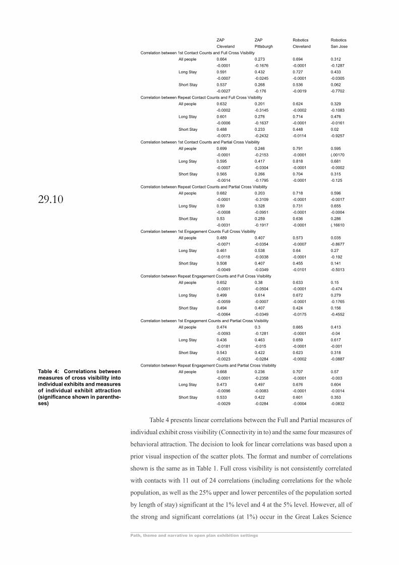
Table 4 presents linear correlations between the Full and Partial measures ofindividual exhibit cross visibility (Connectivity in to) and the same four measures ofbehavioral attraction. The decision to look for linear correlations was based upon aprior visual inspection of the scatter plots. The format and number of correlationsshown is the same as in Table 1. Full cross visibility is not consistently correlatedwith contacts with 11 out of 24 correlations (including correlations for the wholepopulation, as well as the 25% upper and lower percentiles of the population sortedby length of stay) significant at the 1% level and 4 at the 5% level. However, all ofthe strong and significant correlations (at 1%) occur in the Great Lakes Science

ZAP ZAP Robotics RoboticsCleveland Pittsburgh Cleveland San Jose

Correlation between 1st Contact Counts and Full Cross VisibilityAll people 0.664 0.273 0.694 0.312

-0.0001 -0.1676 -0.0001 -0.1287Long Stay 0.591 0.432 0.727 0.433

-0.0007 -0.0245 -0.0001 -0.0305Short Stay 0.537 0.268 0.536 0.062

-0.0027 -0.176 -0.0019 -0.7702Correlation between Repeat Contact Counts and Full Cross Visibility

All people 0.632 0.201 0.624 0.329-0.0002 -0.3145 -0.0002 -0.1083

Long Stay 0.601 0.276 0.714 0.476-0.0006 -0.1637 -0.0001 -0.0161

Short Stay 0.488 0.233 0.448 0.02-0.0073 -0.2432 -0.0114 -0.9257

Correlation between 1st Contact Counts and Partial Cross VisibilityAll people 0.699 0.246 0.791 0.595

-0.0001 -0.2153 -0.0001 (.00170Long Stay 0.595 0.417 0.818 0.681

-0.0007 -0.0304 -0.0001 -0.0002Short Stay 0.565 0.266 0.704 0.315

-0.0014 -0.1795 -0.0001 -0.125Correlation between Repeat Contact Counts and Partial Cross Visibility

All people 0.682 0.203 0.718 0.596-0.0001 -0.3109 -0.0001 -0.0017

Long Stay 0.59 0.328 0.731 0.655-0.0008 -0.0951 -0.0001 -0.0004

Short Stay 0.53 0.259 0.636 0.286-0.0031 -0.1917 -0.0001 (.16610

Correlation between 1st Engagement Counts Full Cross VisibilityAll people 0.489 0.407 0.573 0.035

-0.0071 -0.0354 -0.0007 -0.8677Long Stay 0.461 0.538 0.64 0.27

-0.0118 -0.0038 -0.0001 -0.192Short Stay 0.508 0.407 0.455 0.141

-0.0049 -0.0349 -0.0101 -0.5013Correlation between Repeat Engagement Counts and Full Cross Visibility

All people 0.652 0.38 0.633 0.15-0.0001 -0.0504 -0.0001 -0.474

Long Stay 0.499 0.614 0.672 0.279-0.0059 -0.0007 -0.0001 -0.1765

Short Stay 0.494 0.407 0.424 0.156-0.0064 -0.0349 -0.0175 -0.4552

Correlation between 1st Engagement Counts and Partial Cross VisibilityAll people 0.474 0.3 0.665 0.413

-0.0093 -0.1281 -0.0001 -0.04Long Stay 0.436 0.463 0.659 0.617

-0.0181 -0.015 -0.0001 -0.001Short Stay 0.543 0.422 0.623 0.318

-0.0023 -0.0284 -0.0002 -0.0887Correlation between Repeat Engagement Counts and Partial Cross Visibility

All people 0.668 0.236 0.707 0.57-0.0001 -0.2358 -0.0001 -0.003

Long Stay 0.473 0.497 0.676 0.604-0.0096 -0.0083 -0.0001 -0.0014

Short Stay 0.533 0.422 0.601 0.353-0.0029 -0.0284 -0.0004 -0.0832

Table 4: Correlations betweenmeasures of cross visibility intoindividual exhibits and measuresof individual exhibit attraction(significance shown in parenthe-ses)

29.11


Center, not only for the ZAP but also for the Robotics exhibition. There is no waythat this bias can be reliably interpreted on a small sample of cases. However, weobserve that the temporary exhibition area involved has a compact shape and a clearlydelimited boundary, so as to both encourage cross visibility and filter out extraneousvisual information. Partial cross visibility is more consistently correlated with contactcounts 16 out of 24 correlations significant at the 1% level and another at the 5%level. Once again, the correlations are mostly associated with the Great Lakes ScienceCenter.

Cross visibility has quite powerful effects upon the pattern of engagement.Full cross visibility is correlated with engagement counts with 11 out of 24 correlationssignificant at the 1% level and another 6 at the 5% level. Only in the case of Roboticsat The Tech are no correlations significant. Partial cross visibility is even moreconsistently related with engagement counts with 15 correlations significant at the1% level and another 4 at the 5% level. We draw the conclusion that exhibit crossvisibility affects the pattern of engagement far more than the more generic propertiesof layouts such as direct accessibility or mean depth. Exhibits that become visiblefrom other exhibits stand higher chances of attracting more active engagement.Furthermore, we can perhaps detect an informal pattern of conscious spatial responses.If we look at the comparison between correlations obtained for the people that stayedlonger and those that stayed shorter amounts of time, in 10 out of 16 cases (there are16 pairs of correlations to be compared) the behavior of the people staying longer ismore strongly associated with cross visibility while the pair of correlations comparedare both significant at least at the 5% level. One additional case follows the samepattern but the correlation for people that stayed less time is not significant. In 2cases none of the relevant correlations is significant, while in 2 other cases thebehavior of the people that stayed a shorted length of time is more strongly correlatedwith cross-visibility than the behavior of the people that stayed longer. We concludedthat there is good evidence that as people stay longer, the visibility of individualexhibits from other individual exhibits has a more detectible effect upon decisionsto engage individual exhibits.

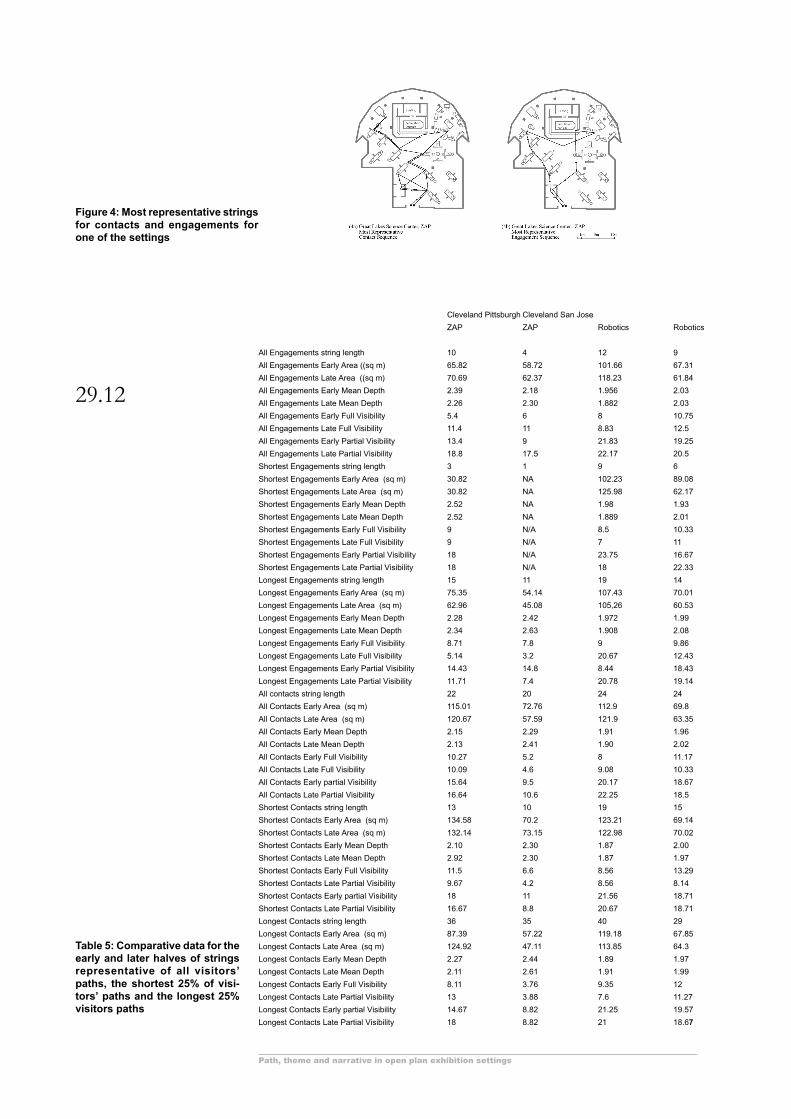
To further establish the basic parameters of our first model, we asked whetherwe could detect any effects of layout upon the sequencing of contacts or engagements.A string matching analysis program, MultiMatch, developed by Conroy-Dalton asan adaptation of the Levenshtein (1965) method of string matching, was used todetermine the most representative paths of the sample at each exhibit site. MultiMatchwas directly made available by its creator who is a member of the research team.The string matching analysis program determines, for any set of strings, the mostrepresentative. The most representative string is defined as the one that would require


29.12

Cleveland Pittsburgh Cleveland San JoseZAP ZAP Robotics Robotics

All Engagements string length 10 4 12 9All Engagements Early Area ((sq m) 65.82 58.72 101.66 67.31All Engagements Late Area ((sq m) 70.69 62.37 118.23 61.84All Engagements Early Mean Depth 2.39 2.18 1.956 2.03All Engagements Late Mean Depth 2.26 2.30 1.882 2.03All Engagements Early Full Visibility 5.4 6 8 10.75All Engagements Late Full Visibility 11.4 11 8.83 12.5All Engagements Early Partial Visibility 13.4 9 21.83 19.25All Engagements Late Partial Visibility 18.8 17.5 22.17 20.5Shortest Engagements string length 3 1 9 6Shortest Engagements Early Area (sq m) 30.82 NA 102.23 89.08Shortest Engagements Late Area (sq m) 30.82 NA 125.98 62.17Shortest Engagements Early Mean Depth 2.52 NA 1.98 1.93Shortest Engagements Late Mean Depth 2.52 NA 1.889 2.01Shortest Engagements Early Full Visibility 9 N/A 8.5 10.33Shortest Engagements Late Full Visibility 9 N/A 7 11Shortest Engagements Early Partial Visibility 18 N/A 23.75 16.67Shortest Engagements Late Partial Visibility 18 N/A 18 22.33Longest Engagements string length 15 11 19 14Longest Engagements Early Area (sq m) 75.35 54.14 107.43 70.01Longest Engagements Late Area (sq m) 62.96 45.08 105,26 60.53Longest Engagements Early Mean Depth 2.28 2.42 1.972 1.99Longest Engagements Late Mean Depth 2.34 2.63 1.908 2.08Longest Engagements Early Full Visibility 8.71 7.8 9 9.86Longest Engagements Late Full Visibility 5.14 3.2 20.67 12.43Longest Engagements Early Partial Visibility 14.43 14.8 8.44 18.43Longest Engagements Late Partial Visibility 11.71 7.4 20.78 19.14All contacts string length 22 20 24 24All Contacts Early Area (sq m) 115.01 72.76 112.9 69.8All Contacts Late Area (sq m) 120.67 57.59 121.9 63.35All Contacts Early Mean Depth 2.15 2.29 1.91 1.96All Contacts Late Mean Depth 2.13 2.41 1.90 2.02All Contacts Early Full Visibility 10.27 5.2 8 11.17All Contacts Late Full Visibility 10.09 4.6 9.08 10.33All Contacts Early partial Visibility 15.64 9.5 20.17 18.67All Contacts Late Partial Visibility 16.64 10.6 22.25 18.5Shortest Contacts string length 13 10 19 15Shortest Contacts Early Area (sq m) 134.58 70.2 123.21 69.14Shortest Contacts Late Area (sq m) 132.14 73.15 122.98 70.02Shortest Contacts Early Mean Depth 2.10 2.30 1.87 2.00Shortest Contacts Late Mean Depth 2.92 2.30 1.87 1.97Shortest Contacts Early Full Visibility 11.5 6.6 8.56 13.29Shortest Contacts Late Partial Visibility 9.67 4.2 8.56 8.14Shortest Contacts Early partial Visibility 18 11 21.56 18.71Shortest Contacts Late Partial Visibility 16.67 8.8 20.67 18.71Longest Contacts string length 36 35 40 29Longest Contacts Early Area (sq m) 87.39 57.22 119.18 67.85Longest Contacts Late Area (sq m) 124.92 47.11 113.85 64.3Longest Contacts Early Mean Depth 2.27 2.44 1.89 1.97Longest Contacts Late Mean Depth 2.11 2.61 1.91 1.99Longest Contacts Early Full Visibility 8.11 3.76 9.35 12Longest Contacts Late Partial Visibility 13 3.88 7.6 11.27Longest Contacts Early partial Visibility 14.67 8.82 21.25 19.57Longest Contacts Late Partial Visibility 18 8.82 21 18.67

Table 5: Comparative data for theearly and later halves of stringsrepresentative of all visitors’paths, the shortest 25% of visi-tors’ paths and the longest 25%visitors paths

Figure 4: Most representative stringsfor contacts and engagements forone of the settings

29.13


the fewest transformations to be changed to represent each of the other route stringsin the sample. Figure 4 shows the most representative contacts and engagementsstrings for one of the settings. In addition to the most representative contact andengagement strings for each setting, we also determined the most representativestrings of the corresponding 50% of the sample that included the longest paths, andthe 50% of the sample that included the shortest paths. Thus, six strings were derivedfor each setting. We checked whether the average Area and the average Mean Depthof the projection polygons corresponding to each node was significantly differentfor the first and second halves of the strings. We found no such tendency. Indeed,strings appeared to oscillate between more and less accessible positions throughouttheir length. Thus, the pattern of accessibility has no strong effect upon the sequencingof exploration and individual exhibit engagement, even though, as we have shownabove, it affects the frequency of contacts.

These results suggest a first conceptualization, or model, of spatial behavioras a function of layout. The most generic, but perhaps less interesting principle isthat direct accessibility affects the distribution of contacts, that is the exposure ofindividual exhibits to visitors, over their search pattern. The less generic, but perhapsmore interesting principle is that as visitors stay longer, they become more aware ofthose individual exhibits that are more visible from other individual exhibits, insuch a way as to decide to engage them. This model would seem to be ratherelementary, and suggests a weakly structured search process. Based on this model,it would appear that good individual exhibit design should provide relativelyautonomous and self contained information at each position, a rather obviousrequirement. More important individual exhibits could be positioned in moreaccessible positions and be made visible from more other individual exhibits inorder to increase the probabilities that they will be contacted and engaged. But asthe properties of layout that affect the probability of contacts or engagements varyindependently of particular path sequences, the model also suggests that goodindividual exhibit design should allow for the additive impact of successiveengagements to be flexible and as much as possible independent of the sequence orindeed the overall set of other individual exhibits that were engaged. This, if accepted,would be a far more demanding requirement but one naturally associated with openand permissive open plans such as those under investigation. However, the enhancedmodel to be developed next, allows us to significantly qualify these statements.


29.14

The compositional model: the statistical effects of labeling and thecognitiveorientation of search paths and engagement patterns.The modified conceptual model to be developed next, arises from analyzing visitors’paths as strings by theme. The question we ask is this: do exhibits carrying the samethematic label appear sequentially within the overall string representing a path, orare they dispersed? We call the corresponding property “categorization”. A string isstrongly categorized if individual exhibits belonging to the same theme occur inuninterrupted sequences and weakly categorized if individual exhibits belonging toone label are interspaced with individual exhibits belonging to other labels.Categorization arises as exhibits are positioned to take into account of each otherand to potentially function as collective and distributed destinations, in ways that donot directly obstruct movement. Hence we call the model to be developed herecompositional, to distinguish it from the positional model in which exhibits are treatedas individual obstructions and destinations.

First, we characterized strings as a whole according to whether they werestrongly or weakly categorized. The aggregate categorization factor of a stringmeasures the extent to which individual exhibits that bear the same label are visitedin succession rather than at dispersed intervals along the path taken by an individualvisitor. The exhibitions were designed in such a way that each exhibit belonged to asingle theme and therefore carried a single thematic label. Higher aggregatecategorization factors indicate that the visitor tended to visit individual exhibitsbearing the same label as a group, before moving to individual exhibits bearinganother label. Aggregate categorization factors are relativized to take into accountthe number of individual exhibits visited per label as well as the total length of thepath (indexed by the number of individual exhibits it encompasses). The formulafor the ACF of a string is:

ACF is the Aggregate Categorization Factork is the number of themes represented in the stringL is the length of the stringT is the number of transitions in the string regardless of themeA is the number of transitions between string nodes belonging to different themesN is the number of members of the theme with the greatest number of members within the string

Examples: For string “EEEEUUCUEE”, k=3, L=10, T=9, A=4, N= 6, L-N=4, N-1=5, Amax= 9-12+10+1=8, Amin=3-1=2, ACF=(8-4)/(8-2)=0.667 For string “EUEU”, k=2, L=4, T=3, A=3, N=2, L-N=2, N-1=1, Amax=3, Amin=1, ACF=(3-3)/(3-1)=0 For string“EEE”, A=0, ACF=1

⊇

if A = 0( ), ACF = 1otherwiseACF =

Amax − A( )Amax − Amin( )

Amin = k −1( )Amax = T,if L − N( ) ? N −1( )Amax = T − 2N + L +1( ),if L − N( ) < N −1( )

29.15


Second, we categorized each label taken separately as being strongly or weaklycategorized within the strings representing visitors’ paths within an exhibition setting.Given the description of visitors’ paths as strings by themes, we defined thecategorization index per label per string as follows:

CL(lg) is the Categorization Index of label “l” in string “g”A(lg) is the number of members of label “l” in the stringS(lg) is the number of segments in which label “l” occursE(lg) is the number of members of label “l” that occur either first or last in the string, and can assume values 0, or 1, or 2. In thespecial case that the string is composed of a single occurrence of label “l”, the value is 2.

Examples: For string “EEEUCU” evaluated for label “C”, A(lC)=1, S(lC)=1, E(lC)=0, 2S(lC -E(lC =2, CL(lC)= (1-1+1)/(2-0)=0.5For the same string evaluated for label “E”, A(lE)=3, S(lE)=1, E(lE)=1, 2S(lE)-E(lE)=1, C(lE)=(3-1+1)/(2-1)=3 For the samestring evaluated for label “U” A(lU)=2, S(lU)=2, E(lU)=1, 2S(lU)- E(lU)=4-1=3, CL(lU)=(2-2+1)/(4-1)=1/3=0.333 For string EEE,evaluated for label “E”, A(lE)=3, S(lE)=1, E(lE)=2, 2S(lE)-E(lE)=2-2=0, CL(lE)=3

The formula essentially provides as with a ratio of string transitions that areinternal to a label “l”, that is transitions which connect two successive individualexhibits belonging to that label, over transitions that are external to a label “l”, thatis transitions which connect an individual exhibit belonging to a label to an individualexhibit not belonging to the same label. The overall Categorization Index for a label,CI(lg) is defined as the average of CI(lg) for all strings “g” in which the label “l”occurs. The analysis of individual strings by labels was done on Excel worksheets.

Plans needed to be similarly analyzed to determine how far individual exhibitsbearing the same thematic label, were spatially adjacent so as to encourage sequentialviewing, or dispersed. We called the property whereby individual exhibits bearingthe same thematic label are spatially adjacent “grouping”. In strongly grouped layouts,individual exhibits belonging to the same label are packed in close adjacency. Inweakly grouped layouts, individual exhibits belonging to the same label are dispersedin different parts of the overall exhibition. A grouping index was developed as follows.First, a Voronoi diagram and Delaunay triangulation was obtained for each layout,after treating each individual exhibit as a point corresponding to its contact region.Delaunay Triangulation was conducted using XYZ GeoBench version 5.05 (freedownloadable software), copyright 1999, P. Schorn, Department of ComputerScience, Swiss Federal Institute of Technology, Zurich. An example is provided infigure 3d. The aim of this exercise was to provide us with a consistent way fordetermining the set of neighbors of each individual exhibit, even though the individualexhibits are irregularly distributed over the layout. Given a set of anchor points

⊇

if A = 0( ), ACF = 1otherwiseACF =

Amax − A( )Amax − Amin( )

Amin = k −1( )Amax = T,if L − N( ) ? N −1( )Amax = T − 2N + L +1( ),if L − N( ) < N −1( )

⊇

if 2S lg( ) − E lg( )( )= 0,CL lg( ) = A lg( )

otherwiseCL lg( ) =

A lg( ) − S lg( ) +1( )2S lg( ) − E lg( )( )


29.16

distributed over an area (here the individual exhibit interface positions) the Voronoidiagram divides space such that each region comprises all other points which areclosest from a given anchor. Thus, the Voronoi diagram provides a convenientconvention for assigning to each individual exhibit a convex polygon territory, suchthat no part of the layout remains unassigned. We do not claim that the Voronoipolygons represent the “attraction area” corresponding to an individual exhibit inany otherwise compelling manner: it is possible that some exhibits are visible andable to attract from well outside the area assigned to them in the Voronoi diagram, asit is also possible that from some positions in that area the specific contents of theexhibits cannot easily be read. The neighbors of an exhibit are unambiguously definedas the set of other exhibits whose Voronoi regions share a boundary with its region.Determining these neighbors if facilitated by considering the Delaunay triangulation,a graph where nodes represent points (here individual exhibit interfaces) and arcsrepresent shared boundaries of corresponding Voronoi regions.

The plans were analyzed to determine the number of Delaunay arcscorresponding to adjacencies between individual exhibits belonging to the samethematic label and the number of Delaunay arcs corresponding to adjacencies betweenindividual exhibits belonging to different thematic labels. Here, the adjacencies underconsideration also represent permeable connections, since we are dealing with openplan layouts. Two grouping indexes were obtained based on the foregoingrepresentations. The individual exhibit-sensitive grouping index, GE(l) for easyreference, is the average of the ratio “internal”/”external” Delaunay arcs, computedfor each set of individual exhibits corresponding to the same label “l”. The label-sensitive grouping index, GL(l) for easy reference, is the ratio “sum of internal”/”sum of external” Delaunay arcs considering all the individual exhibits belonging tothe same label. Thus, GE(l) is an average of ratios, while GL(l) is a ratio of sums.

Table 6 presents the Aggregate Categorization Factors and the average SpatialGrouping Indexes for the four settings. The two Robotics settings have lower valuesfor all factors as compared to the ZAP settings. This indicates a potential associationbetween the spatial grouping of themes and the categorization of visitors’ paths.Given that the small sample of settings does not allow a systematic testing of theimplied association between these variables, the issue is explored further throughthe analysis by themes. The effect of the spatial grouping of labels upon thecategorization of visitors’ paths was analyzed by computing linear correlationsbetween the Categorization Indices and each of the two Grouping Indices for eachlabel. The decision to look for linear correlations was based on a prior visual inspectionof the corresponding scatter plots. These correlations are presented in table 7. Giventhat the number of thematic labels in the exhibitions under study is limited, data

29.17


were analyzed not only by setting but also at different levels of aggregation, in orderto allow for statistical significance in the results. When all settings are considered asa single set, there is a strong and significant correlation between the thematiccategorization of paths and the spatial grouping of layouts. The correlations areeven stronger for engagements than for contacts. This merits some comment. Contactsare to some extent sequenced according to the constraints imposed by layout: it isnot possible to avoid the spaces which mediate between any origin and destinationof a given transition from one individual exhibit of interest to another. Thus, it mighteven be hypothesized that had visitors moved randomly, their contacts would appearthematically categorized in direct proportion to the extent that the plans werethematically grouped. Such a hypothesis could not apply to engagements with similarplausibility. Engagements reflect a conscious decision which is not dictated by thepattern of adjacencies of the layout. The categorization of engagements would,therefore, indicate more clearly a cognitive registration of thematic labels, ascompared to the categorization of contacts. The fact that when data are aggregatedthe spatial grouping of themes affects more powerfully the categorization ofengagements than the categorization of contacts suggests that behaviors reflect thecognitive registration of thematic labels.

When we look at the analysis by setting, correlations between pathcategorization and layout grouping are stronger for the ZAP exhibition settings thanthey are for the Robotics settings. In fact, in the Robotics settings the correlationbetween categorization and grouping is only significant with respect to contacts, notwith respect to engagements. This is consistent with the fact that in the case of theZAP exhibition, thematic labels were not only more clearly grouped spatially, butalso more clearly expressed visually, through the use of color, not only on theindividual exhibits themselves, but also, through projections, in the backgroundsurfaces. However, only 1 of the 16 correlations computed for individual setting issignificant at 1% and only an additional one at 5%. The lack of statistical significance,despite strong correlations, arises from the small number of thematic labels.

The second model developed here suggests that the process of relativelyunstructured and locally driven exploration implied by the first model can be moreglobally and probabilistically constrained by making the thematic organization ofexhibits more evident. This has two kinds of implications. First, it suggests thatdesigners who develop the means to distinguish individual exhibits and also to groupthem spatially according to thematic label, can influence the pattern of visitorexploration. This is of special interest since thematic differentiation can be pursuedwithout imposition of strict exploration sequences. Second, individual exhibit design,and the corresponding layout of knowledge units over an entire exhibition, could

ZAP! ZAP!Surgery Surgery Robotics RoboticsG.t Lakes Carnegie G.t Lakes San JoseScience Science Science TechCenter Center Center Museum

Number of visitors tracked 96 97 103 102Avg. Total Time (minutes) 22.7 15.9 21.1 16.6Avg. Total Stop Time (minutes) 18.8 12.5 17.4 12.8Avg. # of Contacts 28.26 23.80 32.10 23.11Avg. # 1st Contacts per Individual exhibit 48.74 44.44 57.71 60.60%Visitors Contacting each Individual exhibit 51% 46% 56% 59%Avg. # Repeat Contacts per Individual exhibit 92.52 80.78 100.68 98.04Avg. # of Engagements 10.38 6.03 12.51 9.82Avg. # 1st Engagements per Individual exhibit 19.93 13.00 24.74 24.40%Visitors Engaging each Individual exhibit 21% 13% 24% .24%Avg. # Repeat Engagements per Individual exhibit 31.78 17.63 38.55 36.88

Contacts EngagementsALLSTRINGS

GE .551 .605(.0024) (.0006)

GL .67 .693(.0001) (.0001)

ALL ZAP STRINGSGE .471 .616

(.0892) (.0190)GL .638 .713

(.0141) (.0042)ALLROBOTICS STRINGS

GE .721 .408(.0036) (.1480)

GL .582 .391(.0291) (.1670)

ZAPGREAT LAKES SCIENCE CENTER STRINGSGE .221 .644

(.6341) (.1184)GL .462 .707

(.2964) (.0758)ZAP CARNEGIE SCIENCE CENTER STRINGS

GE .715 .586(.0710) (.1665)

GL .798 .725(.0316) (.0654)

ROBOTICS GREAT LAKES SCIENCE CENTER STRINGSGE .691 .338

(.0855) (.4579)GL .621 .416

(.1366) (.3528)ROBOTICS THE TECH STRINGS

GE .887 .515(.0078) (.2371)

GL .723 .470(.0663) (.2874)


29.18

proceed on the assumption that search patterns can either be allowed to repeatedlyintersect thematic groupings, or be channeled more systematically according to thosegroupings. By implication, thematically linked individual exhibits could be treatedas contributing to a more constrained and structured pattern of accumulation ofinformation.

Table 6: Aggregate String Categorization and Spatial Grouping Factorsfor the four Settings

Contacts EngagementsALLSTRINGS GE .551 .605

(.0024) (.0006)GL .67 .693

(.0001) (.0001)ALL ZAP STRINGS

GE .471 .616(.0892) (.0190)

GL .638 .713(.0141) (.0042)

ALLROBOTICS STRINGSGE .721 .408

(.0036) (.1480)GL .582 .391

(.0291) (.1670)ZAPGREAT LAKES SCIENCE CENTER STRINGS

GE .221 .644(.6341) (.1184)

GL .462 .707(.2964) (.0758)

ZAP CARNEGIE SCIENCE CENTER STRINGSGE .715 .586

(.0710) (.1665)GL .798 .725

(.0316) (.0654)ROBOTICS GREAT LAKES SCIENCE CENTER STRINGS

GE .691 .338(.0855) (.4579)

GL .621 .416(.1366) (.3528)

ROBOTICS THE TECH STRINGSGE .887 .515

(.0078) (.2371)GL .723 .470

(.0663) (.2874)

Table 7: Correlations between the grouping ofthemes in the layout and the categorization of pathstrings representing interfaces and stops(significance shown in parentheses)


Contacts: Average Aggregate Categorization Factor 0.546 0.61 0.428 0.355Engagements: Average Aggregate Categorization Factor 0.781 0.771 0.553 0.525Spatial Grouping of Exhibition Theme 60.06% 59.70% 37.35% 48.06%(Individual exhibit Sensitive Index)Spatial Grouping of Exhibition Theme 76.7% 76.7% 50% .35.5%(Theme Sensitive Index)

29.19


DiscussionTwo general methodological and one general theoretical argument can arise fromthe foregoing arguments. The first methodological argument concerns the descriptionof spatial behaviors. Once visitors’ paths are transcribed as strings of variouscharacters, whether representing individual exhibits or themes, the development ofvarious techniques for analyzing the structure of strings is critical to our ability toenrich the systematic description of spatial behaviors. One innovation of the researchreported here is that strings were analyzed not only so that behavioral scores couldbe assigned to particular spatial positions (the individual exhibit interfaces), butalso so that the spatial structure implicit in the string could itself be treated asdescriptive data in its own right. The second methodological argument concerns thedescription of layouts themselves. On the one hand, this description can be refinedthrough the development of more sensitive analytical techniques, such as the analysisof a plan according to the projection polygons that can be generated from a finereference grid overlaid upon it. Software such as Omnivista makes such analysisrelatively easy and such software is increasingly available. On the other hand,however, techniques must also be developed in order to capture how conceptualstructures become embedded in layout design, including conceptual structures thatare expressed through visual form. For example, a set of individual exhibits can begrouped not only by virtue of compact adjacency coupled to label homogeneity, butalso by virtue of being nested inside a spatial region defined through the visualtreatment of the surrounding perimeter, or the elaboration of the ceiling, or indeedlighting, none of which need to literally disrupt movement. Our discussion of themanner in which themes are spatially defined is an elementary step in the directionof developing richer descriptions of exhibition arrangements. There would appearto be much more room for innovation. Future work must not only draw furtherdistinctions between descriptions of the spatial arrangement of individual exhibitswhich take into account various forms of labeling from descriptions which do not,but also continuously test whether descriptions sensitive to labeling can be linked tofunctional implications that can be inferred from observable spatial dimensions ofbehavior.

From a theoretical point of view, it would seem that as we focus on the micro-level of spatial arrangement and behavior in museum environments, the distinctionbetween the positional and the compositional models is fundamental. In a positionalmodel, spatial aspects of behavior are affected by the manner in which boundariesliterally obstruct various kinds of connections of accessibility or visibility in orderto create structures of spatial connectivity or separation, integration or segregation.In a compositional model it is not so much the pattern of literal obstructions thatgenerates spatial structure, but rather the way in which space is configured to stage


29.20

our perception of how objects might be related. From an analytical point of view,cognitive compositioning can initially be conceptualized as the addition ofrelationships between objects which are otherwise equivalent with respect to theirpositioning within a pattern of obstructions to visibility or access. Whether theserelationships arise from common thematic labels associated with consistent coloring,or through the elaboration of lighting, or through decorative means of various sorts(all of which are present in the ZAP exhibition in varying degrees) is immaterial tothis definition.

NotesThe research reported in the article was funded by a National Science Foundation Informal ScienceEducation Grant, #9911829, with Dr. Jean Wineman as Principal Investigator and Dr. John Peponis as coPrincipal Investigator.

ReferencesBenedikt, M. L., 1979, “To Take Hold of Space: Isovists and Isovist Fields”, Environment and Planning

(B), 6, 47-65Choi, Y. K., 1999, "The morphology of exploration and encounter in museum layouts", Environment and

Planning (B): Planning and Design, 26, pp. 241-250Conroy-Dalton, 2001, “The secret is to follow your nose”, in J. Peponis, J. Wineman and S. Bafna (eds.),

Proceedings of the 3rd International Symposium on Space Syntax, Ann Arbor, A. Alfred TaubmanCollege of Architecture and Urban Planning

Levenstein, V. I., 1965, “Binary Codes Capable of Correcting Deletions, Insertions and Reversals”, DikladyAkademii Nauk SSR (Russian), 163 (4), pp. 845-8

Turner, A., Doxa, M., O’Sullivan, D., Penn, A., 2001, “From isovists to visibility graphs: a methodologyfor the analysis of architectural space”, Environment and Planning B: Planning and Design, 28,103-121

Path, theme and narrativein open plan exhibition settingsdiscovery.ucl.ac.uk/1097/1/PTaN.pdf.pdf ·...

Documents

Transcript of Path, theme and narrativein open plan exhibition settingsdiscovery.ucl.ac.uk/1097/1/PTaN.pdf.pdf ·...