
Path Planning Algorithms for Autonomous Border · PDF filePath Planning Algorithms for...
99
Path Planning Algorithms for Autonomous Border Patrol Vehicles by George Tin Lam Lau A thesis submitted in conformity with the requirements for the degree of Master of Applied Science Graduate Department of Aerospace Studies University of Toronto Copyright c 2012 by George Tin Lam Lau
Transcript of Path Planning Algorithms for Autonomous Border · PDF filePath Planning Algorithms for...
Path Planning Algorithms for Autonomous Border PatrolVehicles
by
George Tin Lam Lau
A thesis submitted in conformity with the requirementsfor the degree of Master of Applied ScienceGraduate Department of Aerospace Studies
University of Toronto
Copyright c© 2012 by George Tin Lam Lau
Abstract
Path Planning Algorithms for Autonomous Border Patrol Vehicles
George Tin Lam Lau
Master of Applied Science
Graduate Department of Aerospace Studies
University of Toronto
2012
This thesis presents an online path planning algorithm developed for unmanned vehicles
in charge of autonomous border patrol. In this Pursuit-Evasion game, the unmanned
vehicle is required to capture multiple trespassers on its own before any of them reach a
target safe house where they are safe from capture. The problem formulation is based on
Isaacs’ Target Guarding problem, but extended to the case of multiple evaders. The pro-
posed path planning method is based on Rapidly-exploring random trees (RRT) and is
capable of producing trajectories within several seconds to capture 2 or 3 evaders. Simu-
lations are carried out to demonstrate that the resulting trajectories approach the optimal
solution produced by a nonlinear programming-based numerical optimal control solver.
Experiments are also conducted on unmanned ground vehicles to show the feasibility of
implementing the proposed online path planning algorithm on physical applications.
ii

Acknowledgements
The author would like to thank Dr. Hugh H.T. Liu for his supervision during the past two
years of this research project. In addition, the author would like to acknowledge Jason
Zhang, Sohrab Haghihat, and Keith Leung for their guidance during various stages of
the research.
iii

Contents
1 Introduction 1
1.1 Motivation . . . . . . . . . . . . . . . . . . . . . . . . . . . . . . . . . . . 2
1.2 Objective . . . . . . . . . . . . . . . . . . . . . . . . . . . . . . . . . . . 3
1.3 Overview . . . . . . . . . . . . . . . . . . . . . . . . . . . . . . . . . . . . 5
2 Literature Review 6
2.1 Pursuit-Evasion Games . . . . . . . . . . . . . . . . . . . . . . . . . . . . 6
2.2 Motion Planning . . . . . . . . . . . . . . . . . . . . . . . . . . . . . . . 8
3 Problem Formulation 11
3.1 The Border Patrol Scenario . . . . . . . . . . . . . . . . . . . . . . . . . 11
3.1.1 General Formulation . . . . . . . . . . . . . . . . . . . . . . . . . 11
3.1.2 A Specific Example . . . . . . . . . . . . . . . . . . . . . . . . . . 14
3.2 Evader Control . . . . . . . . . . . . . . . . . . . . . . . . . . . . . . . . 16
3.3 Optimal Control Problem . . . . . . . . . . . . . . . . . . . . . . . . . . 22
4 Algorithms 25
4.1 Rapidly-exploring Random Trees . . . . . . . . . . . . . . . . . . . . . . 26
4.2 Dynamic Programming . . . . . . . . . . . . . . . . . . . . . . . . . . . . 28
4.3 RRT Modification for SP2E . . . . . . . . . . . . . . . . . . . . . . . . . 32
4.3.1 Sampling . . . . . . . . . . . . . . . . . . . . . . . . . . . . . . . 33
iv
4.3.2 Node Connection . . . . . . . . . . . . . . . . . . . . . . . . . . . 34
4.3.3 Cost Estimate . . . . . . . . . . . . . . . . . . . . . . . . . . . . . 35
4.3.4 Rewiring . . . . . . . . . . . . . . . . . . . . . . . . . . . . . . . . 36
4.4 RRT Modification for SP3E . . . . . . . . . . . . . . . . . . . . . . . . . 36
4.4.1 Tree Hybridization . . . . . . . . . . . . . . . . . . . . . . . . . . 39
4.4.2 Rewiring . . . . . . . . . . . . . . . . . . . . . . . . . . . . . . . . 40
5 Simulations 42
5.1 GPOPS . . . . . . . . . . . . . . . . . . . . . . . . . . . . . . . . . . . . 42
5.2 SP2E . . . . . . . . . . . . . . . . . . . . . . . . . . . . . . . . . . . . . . 45
5.3 SP3E . . . . . . . . . . . . . . . . . . . . . . . . . . . . . . . . . . . . . . 49
6 Experiments 53
6.1 Setup . . . . . . . . . . . . . . . . . . . . . . . . . . . . . . . . . . . . . . 53
6.2 Controller Design . . . . . . . . . . . . . . . . . . . . . . . . . . . . . . . 55
6.3 SP2E . . . . . . . . . . . . . . . . . . . . . . . . . . . . . . . . . . . . . . 58
6.4 SP3E . . . . . . . . . . . . . . . . . . . . . . . . . . . . . . . . . . . . . . 62
7 Conclusion 66
7.1 Contribution . . . . . . . . . . . . . . . . . . . . . . . . . . . . . . . . . . 66
7.2 Future Work . . . . . . . . . . . . . . . . . . . . . . . . . . . . . . . . . . 67
A SPSE Target Guarding 68
B C++ SP2E Algorithm 71
C Kalman Filter for Speed Prediction 84
Bibliography 86
v

Nomenclature
P Pursuer
Ei Evader i
x State vector
u Control vector
xP Pursuer’s state vector
xEiEvader i’s state vector
uP Pursuer’s control vector
uEiEvader i’s control vector
zi Mobility of Evader i
X Configuration space
Xb Boundary of configuration space
lb Boundary length (m)
XenterEntry boundary
Xsafe Safe house
rsafe Safe house radius (m)
Xcapt Pursuer’s capture region
rcapt Pursuer’s capture radius (m)
xP Pursuer’s x-coordinate (m)
yP Pursuer’s y-coordinate (m)
vP Pursuer’s speed (m/s)
vi

θP Pursuer’s heading input (rad)
xEiEvader i’s x-coordinate (m)
yEiEvader i’s y-coordinate (m)
vE Evader’s speed (m/s)
θEiEvader i’s heading input (rad)
k Pursuer-evader speed ratio
JP Pursuer’s objective function
JEiEvader i’s objective function
φ Terminal cost/objective
L Time-integral cost/objective
λ Costate vector
H Hamiltonian
ψ Terminal constraint
ν Terminal constraint multiplier
Border Patrol Algorithm Nomenclature:
V Node set
E Edge set
Xnear Set of locations of nearby nodes
V π Expected total reward for following control policy π
πS One-by-one SPSE pursuit policy
zc Compact representation of evader mobility
Experiment Nomenclature:
FV Vicon inertial reference frame
FR Robot reference frame
xg Goal state
vii

FG Goal inertial reference frame
θV Robot heading, Vicon frame
e Pose error, Robot frame
K Control matrix
v Translational speed (m/s)
ω Rotational speed (rad/s)
r Vector from robot to goal
ρ Distance between robot and goal (m)
α Angle between r and x-axis of FR (rad)
β Angle between r and x-axis of FG (rad)
viii

Chapter 1
Introduction
Pursuit-Evasion games are a family of problems where a class of agents, called pursuers,
are assigned the task of capturing another class of agents, called evaders, in a given
environment. Research in this topic is widespread and delves into many variations of the
Pursuit-Evasion game, including the number of pursuers and evaders, the cost function by
which performance is measured, the movement and sensing capabilities of the agents, and
the environment in which the game is played. The problem of Pursuit-Evasion applies in
many situations. When building security is breached, searchers must sweep the different
corridors and rooms of the building and locate the intruder without letting it escape.
Search and rescue operations are variants of the Pursuit-Evasion problem where a team
of vehicles must search an unknown environment to track down lost individuals. Military
operations requiring the capture of various agents using Unmanned Aerial Vehicles (UAV)
are also related to Pursuit-Evasion problems. Another potential application of this field
of research is automated border patrol, which is the focus of this thesis.
The automated border patrol scenario has several defining features that distinguish
it from most research in Pursuit-Evasion problems. Due to the vast search area involved
in patrolling a national border, assigned agents would be spread out very far apart from
each other. When illegal entry occurs and individuals trespass upon the area, the agent(s)
1

Chapter 1. Introduction 2
in closest proximity must capture all the evaders before they can reach a target location,
such as a dense forest or urban area, where tracking becomes much more difficult. The
unique features of this problem are: 1) a few pursuers attempting to capture multiple
evaders, and 2) the evaders having a target destination that they attempt to reach where
they will be safe from the pursuer upon arrival. The border patrol scenario is set up
with these features to represent the use of a UAV for autonomously patrolling a national
border. Because of the lengths of the Canada-U.S. and U.S.-Mexico borders, using a
system of UAVs would be a significant improvement over human patrol teams in terms
of cost, range, and efficiency.
1.1 Motivation
The utilization of UAVs for border patrol is not a novel concept. In 2005, the U.S.
Department of Homeland Security’s Customs and Border Protection began using the
MQ-9 Predator B UAVs as part of their taskforce for patrolling the U.S.-Mexico border1.
This was part of a new security initiative known as SBInet where technological solutions
were to be set up to monitor the area2. However, after four years, the $4 billion spent
amounted to a system covering only 28 miles, or 1.8% of the border3.
Despite the setbacks, the UAV portion of the project was the lone bright spot of the
system. While the overall SBInet project has been halted, more UAVs are being added
for border surveillance, with the expectation that 24 Predator drones will be in operation
1P. McLeary. ”New Technologies Aid Border Patrol.” Internet: http://www.aviationweek.
com/aw/generic/story_generic.jsp?channel=dti&id=news/dti/2010/11/01/DT_11_01_2010_
p37-262578.xml&headline=null&next=10, Nov. 2010 [Mar. 26, 2011].2”U.S. Customs and Border Protection - Border Security.” Internet: http://cbp.gov/xp/cgov/
border_security/sbi/sbi_net/, Dec. 2009 [Mar. 26, 2011].3C. McCutcheon. ”Securing Our Borders.” Internet: http://www.americanprogress.org/issues/
2010/04/secure_borders.html, Apr. 2010 [Mar. 26, 2011].

Chapter 1. Introduction 3
by 20164. The relatively low $16-million cost of the UAV5 makes them a cost-efficient
and flexible solution for border security. However, existing ones are manually operated
and serve only as a complement to ground agents. The proposed research will provide a
guidance system for pursuing and capturing trespassers so that UAVs can autonomously
complete the task without the aid of human patrol teams.
1.2 Objective
Here, we address a multi-agent Pursuit-Evasion game where a single pursuer, representing
an unmanned vehicle, is patrolling a border and is responsible for capturing multiple
evaders before they are able to arrive at a target destination. The goal of this thesis is
to develop a guidance system that generates a trajectory for the pursuer to efficiently
capture these border trespassers. In order to have a guidance system that is practical
and can be implemented on physical applications, several requirements must be met:
• The guidance system must be able to generate a trajectory for the pursuer to
follow in real-time (i.e. within several seconds of receiving information regarding
the position of the trespassers)
• The guidance system must be able to operate under a wide range of scenarios (i.e.
variations in initial positions, maximum speed, and vehicle capture capabilities)
• The guidance system must generate trajectories that are close to the optimal solu-
tion
Current research for finding solutions to Pursuit-Evasion games have typically been
analytical or heuristic in nature, which limits their ability to satisfy the above require-
4W. Booth. ”More Predator drones fly U.S.-Mexico border.” Internet: http://www.
washingtonpost.com/world/more-predator-drones-fly-us-mexico-border/2011/12/01/
gIQANSZz8O_story.html, Dec. 2011 [Jun. 22, 2012].5J. Hing. ”Aerial Drones Take Over the Border.” Internet: http://colorlines.com/archives/
2010/09/aerial_drones_take_over_the_border.html, Sept. 2010 [Mar. 26, 2011].

Chapter 1. Introduction 4
ments. Analytical solutions are favorable and would yield guidance laws that can produce
desired trajectories in real-time, but unfortunately, such solutions are available only to the
simplest types of problems. Isaacs, in his pioneering work Differential Games provided
minimax solutions for several Single-Pursuer, Single-Evader (SPSE) zero-sum problems
[1]. Analytical solutions have also been found for several other SPSE problems, which
will be presented in the next chapter. For more complex problems, such as problems
with more than one pursuer and/or evader, complicated cost functions, or cluttered or
changing environments, analytical solutions are often intractable. Heuristic methods are
then used in such cases in two ways: to reduce the problem into simpler, manageable
ones, or to generate a pursuit strategy in itself. Such heuristic solutions use human ex-
perience to generate better strategies, but it is difficult to determine whether they are
generating trajectories that are close to the minimax solution or not.
Due to the solution requirements, the nature of the problem, and the limits of current
solutions for Pursuit-Evasion games, the challenges in developing a suitable guidance
system for this application are:
• Having multiple evaders in the problem increases the complexity of the problem
• Contrary to most Pursuit-Evasion problems studied, where the cost/objective func-
tion is the time to capture, the pursuer’s cost function is a function of the distance
of the evaders from the goal when they are captured
• The cost/objective function will be different for the pursuer than the evaders, re-
sulting in a non-zero-sum problem
• When an evader is captured, it is immobilized, resulting in a change of vehicle
dynamics and hence creating a multi-stage problem that must be solved
As mentioned before, while analytical solutions are definitely the most appealing, the
complexity of this problem suggests that developing a numerical solution would be more

Chapter 1. Introduction 5
practical. The algorithm developed in this thesis for the border patrol Pursuit-Evasion
problem is a sampling-based motion planner based on robot path-planning methods. The
rest of this thesis will be devoted to explaining the concept behind this algorithm and
demonstrating the feasibility in implementing the proposed guidance system for physical
applications.
1.3 Overview
The rest of the thesis is organized as follows. Chapter 2 provides a literature review on
existing research on Pursuit-Evasion games as well as robot motion planning algorithms.
In Chapter 3, the border patrol problem is presented for autonomous vehicles. Simpli-
fying assumptions concerning the problem are also explained - assumptions based on
Isaacs’ Target Guarding problem [1] that reduce the problem from a differential games
problem to an optimal control problem. In Chapter 4, the algorithms developed for the
autonomous vehicle border patrol scenario are presented. Simulation results using the
algorithms are provided in Chapter 5 for different test cases and compared to offline
trajectories generated by existing numerical optimal control solvers to show that the al-
gorithms achieve near-optimal solutions. In Chapter 6, experimental method and results
using autonomous ground vehicles are presented to demonstrate the algorithms in use for
physical applications. To conclude, a summary of the research completed and possible
future work are given in Chapter 7.

Chapter 2
Literature Review
This chapter summarizes the existing and current research on Pursuit-Evasion games
in general. From this, we show the lack of research and understanding in problems
related to the border patrol scenario, including multiple-player problems and non-zero-
sum problems. Since the border patrol algorithm proposed in Chapter 4 is based on path
planners developed in the field of robotics, a review of different types of motion planning
algorithms and recent development of particular algorithms of interest is provided.
2.1 Pursuit-Evasion Games
Isaacs’ Differential Games was the first comprehensive study of the topic of Pursuit-
Evasion games. Approaching the problem from a purely mathematical perspective, he
derived analytical solutions for several examples, such as the Homicidal Chauffeur prob-
lem and the Isotropic Rocket problem [1]. His study was focused on Single-Pursuer,
Single-Evader (SPSE) problems where the opposing players were trying to minimize
and maximize the same objective function, respectively. These are known as zero-sum
problems and lead to the notion of minimax solutions, where each player optimizes its
objective while considering the other player’s attempt to achieve the opposite. Analyt-
ical studies have also been conducted on singular and universal surfaces that define the
6
Chapter 2. Literature Review 7
convergence of optimal paths [1, 2].
Unless it is assumed that the pursuer has complete visibility of the entire environment,
Pursuit-Evasion problems are usually divided into two stages: searching and pursuing
the evader. For the search stage, discrete probabilistic frameworks have been developed
in the case where pursuers’ sensor readings may be erroneous [3, 4, 5]. Randomized
sampling-based algorithms have been proposed where the environment is divided into
different roadmaps for searching [6, 7]. The set of possible current locations for previously
detected evaders that have escaped the pursuer’s visibility region has also been studied
[8].
For the pursuit phase, analytical solutions have been found for several SPSE problems,
including a stochastic differential game based on Dubins’ car model [9] and a bounded
game for an interceptor missile [10]. There has also been research done that deals with
problems with obstacles in the environment and multiple players. Maintaining visibility
of evaders around obstacles was addressed [11, 12, 13]. Evolutionary algorithms have
been applied in Pursuit-Evasion games as well [14].
When dealing with multiple pursuers and evaders, the problem becomes more com-
plex. As analytical solutions for such cases are intractable, there have been numerical
solutions where the problem is broken down into several SPSE problems, with periodic
assessments of the global problem at preset intervals [15, 16]: the SPSE engagements are
evaluated, and if deemed to be inefficient, the engagements are reassigned [15]. Particle
swarm optimization has also been proposed for multiple pursuers trying to capture a
single pursuer [17]. Research in SPME problems is scarce; geometry bounds on capture
regions have been studied for basic problems [18], but no solution has yet been developed.
Other guidance laws developed for multiple-pursuer or multiple-evaders problems have
been mostly heuristic in nature. These include the planes strategy where the pursuers
form a semi-circle to contain the evader [19], a frontier-based search to trap the evader
[20], assigning guards [21], and reducing sensor overlap [22].

Chapter 2. Literature Review 8
If the pursuer and evader are optimizing over different objective functions, the problem
becomes a non-zero-sum differential game. Theory on the existence and determination of
equilibrium points is not as developed as those for zero-sum problems [23, 24]. Optimal
solutions have been found for the linear-quadratic case [25], but besides this, most studies
on this specific topic have been preliminary in nature [23, 26, 27].
2.2 Motion Planning
Robot motion planning in the presence of obstacles has been a hot topic of research in
recent years, and this has led to the development of many types of solution methods. Of
these appraches, several notable classes of algorithms include roadmap methods, cell de-
composition methods, potential field methods, and sampling-based planning. Roadmap
methods decompose the free space into a graph by incrementally building a map of it as
data about the environment is gathered from the robot’s sensors [28]. Visibility graphs,
Voronoi roadmaps, and silhouette methods are instances of roadmap planners. Most of
these methods are limited to two or three dimensions [29].
Cell decomposition methods also decompose the configuration space for the purpose
of finding an obstacle-free trajectory via graph search, but rather than fitting a graph
onto the free space, it is split into a finite number of cells, with the boundaries of the cells
usually representing the change in an obstacle’s geometry or the visibility due to that
obstacle [28]. Some decomposition methods include trapezoidal, critical-curve based, and
tree decomposition [29].
Potential field methods map a potential function to the free space so that the vehicle
will move in reaction to the forces defined by this field. In obstacle avoidance, obstacles
are assumed to emit repulsive forces like that of an electric charge in order to drive the
vehicle away from it [30]. The trajectory can be generated by the potential function via
gradient descent, but the existence of local minima is a potential problem of such an
Chapter 2. Literature Review 9
approach. Possible solutions to this problem are to use a wave-front planner on a grid
similar to dynamic programming or to define a navigation potential function that only
has one minimum [28].
All the methods described so far require an explicit representation of the free space,
leading to computational inefficiency as the dimensionality increases. Sampling-based
methods avoid this by building a map of the environment by incrementally sampling
random new points, checking the validity of the new points by a collision detection
module, and connecting them to existing ones in the map if valid [31]. The way in which
points are connected vary based on the method applied, but the common feature is that
connections are made between two selected points if the path between them is obstacle-
free, and rejected otherwise. Sampling-based planners have the ability to incorporate
vehicle differential constraints into its state space search [29].
In the border patrol scenario, sampling-based methods are more suitable for appli-
cation to this problem. Of particular interest is the Rapidly-exploring Random Tree
(RRT), a sampling-based method that uses a tree structure to store and connect the
sample points in the configuration space. First developed by LaValle and Kuffner [32]
and shown to be probabilistically complete [33], it was then extended to deal with system
dynamics [34]. Since then, the RRT algorithm has been modified for different purposes,
including optimal motion planning [35], multiple-UAV obstacle avoidance [36], and urban
driving [37]. Recently, RRTs have also been applied to a Pursuit-Evasion problem, where
an algorithm was developed for an evader trying to reach a goal while avoiding multiple
slower pursuers [38].
In summary, the Rapidly-exploring Random Tree is a sampling-based method for
robot motion planning that is more flexible for modification for the border patrol problem
of interest. It is superior in this respect over other motion planning algorithms as it
doesn’t require an explicit representation of the problem for it to plan paths for the
robot. The reason for turning to motion planning algorithms is because of a lack of

Chapter 2. Literature Review 10
existing research on Pursuit-Evasion games dealing with properties in the border patrol
scenario, namely problems with a single pursuer and multiple evaders and non-zero-sum
problems. While there have been studies done for simple cases of such problems, most
Pursuit-Evasion studies have been focused on analytical studies of SPSE problems and
heuristic strategies for problems with multiple pursuers and/or evaders.

Chapter 3
Problem Formulation
In this chapter, the formulation of the border patrol Pursuit-Evasion problem of interest
is presented, beginning with a general description and followed by a specific instance
for which simulations and experimental results are included in subsequent sections. The
procedures involved in developing simplifying assumptions about the evaders’ dynamics
based on Isaacs’ Target Guarding Problem are then introduced, followed by a description
of the resulting optimal control problem whose objective function we seek to optimize by
selecting a proper control input for the pursuer.
3.1 The Border Patrol Scenario
3.1.1 General Formulation
The dynamics of the pursuer P and evaders Ei in the problem is governed by the set of
differential equations
xP = fP (xP ,uP ), xP (0) = xP,0 (3.1)
xEi= fEi
(xEi,uEi
), xEi(0) = xEi,0 (3.2)
11
Chapter 3. Problem Formulation 12
where xP and uP are the state and control vectors of the pursuer and xEiand uEi
are
the state and control vectors of evader i. Assuming the players exist in Rd physical space
with dimensionality d = 2 or 3, let
xP =
[xpos,P xdyn,P
]T, xpos,P ε Rd (3.3)
xEi=
[xpos,Ei
xdyn,Ei
]T, xpos,Ei
ε Rd (3.4)
such that xpos,P and xpos,Eicontain the states describing P and Ei’s positions in physical
space, and xdyn,P and xdyn,Eicontain additional states necessary to describe P and Ei’s
dynamics (e.g. velocity, heading). Then, restrict xpos,P and xpos,Eito remain in the
closed set X ⊂ Rd over some finite horizon t ε [0, tf ]. The equations of motion for Ei can
be decomposed as follows:
xEi=
xpos,Ei
xdyn,Ei
= fEi(xEi
,uEi) =
zi · fpos,Ei(xEi
,uEi)
fdyn,Ei(xEi
,uEi)
(3.5)
zi represents the mobility of evader i, and takes the values 1 (evader is active) and 0
(evader is immobilized). For a game with n evaders, the full state and control vectors of
the problem would be
x =
[xP xE1 · · · xEn
]T(3.6)
u =
[uP uE1 · · · uEn
]T(3.7)
Likewise, the full set of differential equations would be

Chapter 3. Problem Formulation 13
x =
fP (xP ,uP )
fE1(xE1 ,uE1)
...
fEn(xEn ,uEn)
(3.8)
Letting Xb be the boundary of X and Xenter ⊂ Xb represent the border through
which the evaders trespass into X, the initial positions of the pursuer and evader i are
given by xpos,P (0) ε X and xpos,Ei(0) ε Xenter respectively. The mobility functions zi are
all initially set to 1. The evaders seek to enter into the subset Xsafe ⊂ X representing
the safe house, while the pursuer attempts to capture and immobilize them before any
evaders can arrive at Xsafe.
Capture of evader i occurs at time tcapt,i when
xpos,Ei(tcapt,i) ε Xcapt(xP (tcapt,i)), tcapt,i ε [0, tf ] (3.9)
Xcapt ⊂ X is a set pinned to and moves with xP , analogous to a rigid body in dynamics.
It represents the region surrounding P for which any evader entering it is within range
for the pursuer to instantly capture it. Upon capture, Ei is immobilized, and zi assumes
the value of 0 for all t ≥ tcapt,i.
There are two termination conditions for this finite-horizon problem, one correspond-
ing to the success of the pursuer in capturing all the evaders before any of them arrive
at Xsafe, and the other corresponding to its failure in doing so. The success criteria at
tf can be expressed as
∀i = 1, . . . , n, zi(tf ) = 0 (3.10)
and the failure criterion as
∃ i ε 1, . . . , n s.t. xpos,Ei(tf ) ε Xsafe (3.11)
Chapter 3. Problem Formulation 14
The objective functions of the evaders are their respective Euclidean distances away
from the closest point in Xsafe when the problem terminates:
JEi(xEi
(tf )) = minxsεXsafe
‖xpos,Ei(tf )− xs‖, i = 1, . . . , n (3.12)
In turn, the objective function of the pursuer is the closest Euclidean distance of any of
the evaders away from the closest point in Xsafe when the problem terminates:
JP (x(tf )) = mini=1,...,n
JEi(xEi
(tf )) (3.13)
The problem is then one where the evaders seek to minimize their own objectives,
minuEi
JEi(xEi
(tf )), i = 1, . . . , n (3.14)
while the pursuer seeks to maximize its objective,
maxuP
JP (x(tf )) (3.15)
Note that there is no time-integral cost in the objective function, and that the problem
is non-zero-sum.
3.1.2 A Specific Example
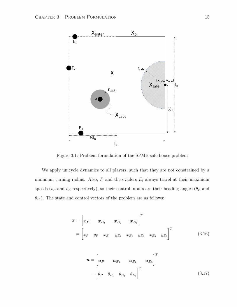
Consider the problem in Figure 3.1. X ⊂ Rd is a square space of length lb with boundary
Xb. At t = 0, evaders E1, E2, and E3 are located on Xenter, the dashed left-half portion
of Xb. Their individual goals are to reach Xsafe, a semi-circle of radius rsafe attached
to the right side of X with its center located at (xsafe, ysafe). At t = 0, P is in X and
attempts to capture all three evaders before any of them arrive at Xsafe. P has a circular
capture region, denoted by Xcapt, of radius rcapt with its center at pos(xP ) for which all
evaders entering it are assumed to be captured and immobilized.
Chapter 3. Problem Formulation 15
Figure 3.1: Problem formulation of the SPME safe house problem
We apply unicycle dynamics to all players, such that they are not constrained by a
minimum turning radius. Also, P and the evaders Ei always travel at their maximum
speeds (vP and vE respectively), so their control inputs are their heading angles (θP and
θEi). The state and control vectors of the problem are as follows:
x =
[xP xE1 xE2 xE3
]T=
[xP yP xE1 yE1 xE2 yE2 xE3 yE3
]T(3.16)
u =
[uP uE1 uE2 uE3
]T=
[θP θE1 θE2 θE3
]T(3.17)
Chapter 3. Problem Formulation 16
The differential equations governing the pursuer’s dynamics are:
xP =
xPyP
=
vP cos θP
vP sin θP
(3.18)
while the differential equations governing the evaders’ dynamics are:
xE1 =
xE1
yE1
=
z1 · vE cos θE1
z1 · vE sin θE1
(3.19)
xE2 =
xE2
yE2
=
z2 · vE cos θE2
z2 · vE sin θE2
(3.20)
xE3 =
xE3
yE3
=
z3 · vE cos θE3
z3 · vE sin θE3
(3.21)
As Xsafe is a semi-circular region attached to the right edge of X, the following are
the objective functions of evader i and the pursuer respectively:
JEi(xEi
(tf )) =√
(xsafe − xEi(tf ))2 + (ysafe − yEi
(tf ))2 − rsafe, i = 1, 2, 3 (3.22)
JP (x(tf )) = mini=1,2,3
JEi(xEi
(tf )) (3.23)
This specific instantiation of the border patrol problem will be studied for the re-
mainder of this thesis. In Chapter 4, the algorithms developed will be for this particular
scenario consisting of either two or three evaders.
3.2 Evader Control
With the current problem formulation, finding an optimal solution for the pursuer’s
control also requires simultaneously finding a solution for the evaders’ controls as well.
Chapter 3. Problem Formulation 17
This is known as a differential games problem, which is similar to the problems studied
in game theory, except in a continuous setting. The solution to such problems are called
minimax solutions, where any deviation for either the pursuer(s) or evader(s) from the
strategy presented by the minimax solution will lead to that party doing worse than if it
didn’t deviate. There currently does not exist any methods, analytical or numerical, for
solving the general class of differential games.
In light of the intractability in finding an online algorithm to produce the minimax
solution to this differential games problem, it is beneficial, both in terms of being able
to generate a solution and computational cost, to first find a reasonable control law of
the evaders. Knowing or having a good approximation of their behavior converts the
differential games problem into an optimal control problem.
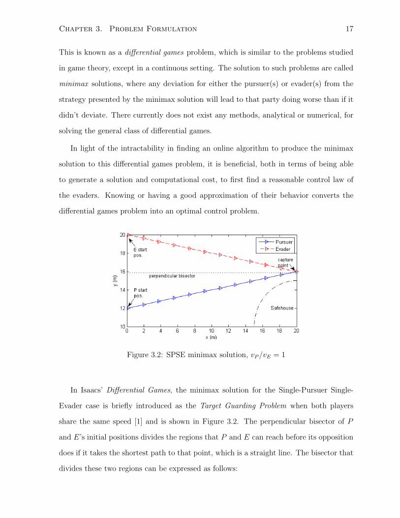
Figure 3.2: SPSE minimax solution, vP/vE = 1
In Isaacs’ Differential Games, the minimax solution for the Single-Pursuer Single-
Evader case is briefly introduced as the Target Guarding Problem when both players
share the same speed [1] and is shown in Figure 3.2. The perpendicular bisector of P
and E’s initial positions divides the regions that P and E can reach before its opposition
does if it takes the shortest path to that point, which is a straight line. The bisector that
divides these two regions can be expressed as follows:
Chapter 3. Problem Formulation 18
ydiv(x) = −xE − xPyE − yP
x+1
2(yP + yE +
x2E − x2PyE − yP
) (3.24)
The minimax strategy for both players is to travel in a straight line from its initial position
to the point on the bisector closest to Xsafe. Any trajectory for P and E that deviates
from this strategy would not be optimal and will lead to capture closer to or further away
from the Xsafe, respectively, assuming that its opponent follows the minimax strategy.
In the example presented in 3.1.2, the closest point on the bisector to Xsafe is
x∗ =xsafe + 1
2(xE−xPyE−yP
)
1 + (xE−xPyE−yP
)2· (yP + yE − 2ysafe +
x2E − x2PyE − yP
) (3.25)
y∗ = ydiv(xminmax) (3.26)
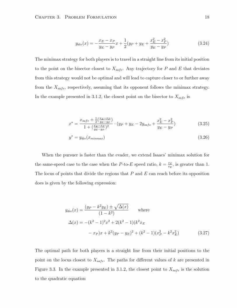
When the pursuer is faster than the evader, we extend Isaacs’ minimax solution for
the same-speed case to the case when the P -to-E speed ratio, k = vPvE
, is greater than 1.
The locus of points that divide the regions that P and E can reach before its opposition
does is given by the following expression:
ydiv(x) =(yP − k2yE)±
√∆(x)
(1− k2)where
∆(x) = −(k2 − 1)2x2 + 2(k2 − 1)(k2xE
− xP )x+ k2(yP − yE)2 + (k2 − 1)(x2P − k2x2E) (3.27)
The optimal path for both players is a straight line from their initial positions to the
point on the locus closest to Xsafe. The paths for different values of k are presented in
Figure 3.3. In the example presented in 3.1.2, the closest point to Xsafe is the solution
to the quadratic equation
Chapter 3. Problem Formulation 19
ax∗2 + bx∗ + c = 0, where
a = (k2 − 1)2[((k2 − 1)ysafe + yP − k2yE)2 + (k2xE − xP − (k2 − 1)xsafe)2]
b = (k2 − 1)[−2((k2 − 1)ysafe + yP − k2yE)2(k2xE − xP )
− 2(k2xE − xP − (k2 − 1)xsafe)2(k2xE − xP )]
c = ((k2 − 1)ysafe + yP − k2yE)2(k2xE − xP )2
− (k2xE − xP − (k2 − 1)xsafe)2(k2(yP − yE)2 + (k2 − 1)(x2P − k2x2E)) (3.28)
Figure 3.3: SPSE minimax solution, vP/vE > 1
For the rest of this section, the solutions just presented in Equations 3.24-3.28 will be
referred to as the geometric solution. To confirm that this geometric solution is indeed
the minimax solution to the zero-sum problem, consider the following solution technique
presented by Isaacs for general zero-sum differential games. Given n state equations
x = f(x, uP , uE) and the objective function
J = φ(xf , tf ) +
∫ tf
0
L(x, uP , uE)dt (3.29)
that the pursuer and the evader seek to maximize and minimize, respectively, define the
Hamiltonian with costates λ

Chapter 3. Problem Formulation 20
H(x, uP , uE) = L+ λT (t) · f(x, uP , uE) (3.30)
In order to find the minimax solution, Isaacs’ technique is to define a parametric
surface representing the terminal states of the problem, and integrate backwards in time
starting from this surface. Although this will not yield an analytical solution that provides
a control law, the trajectories generated can be compared with those generated by the
geometric solution proposed earlier. If the trajectories from the two solutions coincide,
then the geometric solution is indeed the minimax solution.
For the rest of this thesis, any function that is superscripted with an asterisk (e.g.
u∗) indicates the minimax or optimal value that function can attain. Isaacs states that
the minimax solution imposes the following condition, known as Isaacs’ Main Equation
[2]:
H∗(xf , uP,f , uE,f , λf ) = 0 (3.31)
Also, the evolution of the costates in the minimax solution are governed by the fol-
lowing differential equations:
λ(t) = −∂H∗
∂x(3.32)
The costate and state differential equations form 2n equations that must be integrated
over time to yield the minimax trajectory. This requires 2n final conditions at the
terminal state. The choice of the final states to begin backwards integration over time
provides n such conditions, while Eq. 3.31 provides another condition. Additionally,
define the n − 1 dimensional parametric surface representing the terminal states by the
following:
xi = hi(s1, . . . , sn−1), i = 1, . . . , n (3.33)

Chapter 3. Problem Formulation 21
The partial derivative of the terminal objective φ with respect to the parametric
surface obeys the following equalities:
∂φ
∂sk=
n∑i
λi∂hi∂sk
, k = 1, . . . , n− 1 (3.34)
Eq. 3.34 provides the remaining n−1 equations required for the final conditions. The
details of this solution technique applied to the SPSE problem for different speeds can
be found in Appendix A. Results of the solution trajectory generated by this backward
integration technique and that generated by the geometric solution proposed earlier for
the same initial conditions are compared in Fig. 3.4 for speed ratios of 1 and 1.5. As can
be seen, the trajectories are identical, confirming that the geometric solution does indeed
provide the minimax control law.
(a) vP /vE = 1 (b) vP /vE = 1.5
Figure 3.4: Comparison of the trajectories generated by the control law and Isaacs’
solution technique different pursuer-evader speed ratios. The circles indicate the initial
positions of the agents, while the crosses indicate the capture points.
This is a reasonable model of the evaders’ control inputs as the evaders are non-
cooperative and seek only to maximize its own objective without any consideration of
Chapter 3. Problem Formulation 22
the other evaders’ objectives. Using Isaacs’ minimax strategy is the best that each evader
can do in the one-on-one case. Granted, it is possible that border trespassers may deviate
from this strategy, but as this model is an optimal representation of the SPSE safe house
problem, it will allow the pursuer to perform even better in most cases when the evader
opts for a different control law.
Note that the minimax strategy only applies when the evader’s reachable region does
not contain any part of Xsafe (i.e., the pursuer is guaranteed to capture the evader if it
employs the minimax strategy). In the case where the evader’s reachable region contains
some or all of Xsafe, the evader’s control law would be to move in a straight line towards
the closest point on Xsafe that it can safely reach. Define the evader’s ability to safely
reach the safe house as
σi =
1, ∃ xsafe ε Xsafe s.t. vPvE· ‖xEi
− xsafe‖ < ‖xP − xsafe‖
0, otherwise(3.35)
Then, the evader’s heading is given as
θEi=
tan−1(y∗−yEi
x∗−xEi
), σi = 0
tan−1(ysafe−yEi
xsafe−xEi
), σi = 1
(3.36)
3.3 Optimal Control Problem
With a control law for the evaders in place, the problem is now an optimal control
problem in terms of the pursuer’s control input. The problem is governed by the m state
equations x = f(x, u, t) given in Eq. 3.8 with m initial conditions x0, and we are trying
to maximize the following objective function, upon substituting Eqs. 3.12 and 3.13, with
respect to the control input u:
Chapter 3. Problem Formulation 23
JP = φ(xf , tf ) +
∫ tf
0
L(x, u, t)dt, L(x, u, t) = 0
= mini=1,...,n
JEi(xEi,f )
= min{ minxsεXsafe
‖xpos,E1 − xs‖, . . . , minxsεXsafe
‖xpos,En − xs‖} (3.37)
The problem is a free-time problem with terminal constraints, meaning there is no
fixed time at which the problem ends, but it ends when specified conditions are met.
Assuming that we are not interested in situations where the pursuer fails to capture the
evaders before they reach the safe house (for which the objective function would have no
quantitative meaning), the success terminal condition, by expressing Eq. 3.10 in another
format, is as follows:
ψ(xf,tf ) =n∑i=1
zi(tf ) = 0 (3.38)
Define the Hamiltonian with costates λ
H = L+ λT (t) · f(x, u, t)
=
[λ1 · · ·λm
]·
fP (xP ,uP )
fE1(xE1 ,uE1)
...
fEn(xEn ,uEn)
(3.39)
The m costate equations of the problem are
λ(t) = −∂H∂x
(3.40)
We also have a terminal constraint multiplier ν that does not change over time, ie.
ν = 0 (3.41)

Chapter 3. Problem Formulation 24
For optimality (ie. the control input u is optimal), the m costates are governed by the
following end-point conditions (we will from this point on denote all optimal conditions
with an asterisk):
λ∗(tf ) =∂φ(xf,tf )
∂x+∂ψ
∂x· νT (3.42)
As this is a problem with free final time, an additional terminal condition is imposed on
the Hamiltonian
H(xf,uf,tf,λf ) +∂φ(xf,tf )
∂t+ νT · ∂ψ(xf,tf )
∂t= 0 (3.43)
whereas the stationarity condition for a solution extrema is given by
∂HT
∂u= 0 (3.44)
Finally, to confirm that the extrema is a maxima, the following condition must be met:
∂2HT
∂u2< 0 (3.45)
Although the border patrol algorithm proposed in the next chapter is not based
on the standard optimal control problem formulation explained above, it is nonetheless
important to outline this framework. In Chapter 5, the trajectories generated by the
algorithm developed in this thesis are compared with those generated by the GPOPS
numerical optimal control solver, which checks its solution with the optimality conditions
presented here.

Chapter 4
Algorithms
In the previous chapter, the Pursuit-Evasion problem was presented and, using differential
game theory to make assumptions about the evaders’ control law, was modified into an
optimal control problem. Although numerical optimal control methods exist in literature
and in practice, they may require significant computational resources, do not provide
convergence guarantees to a feasible trajectory, and generally require an initial guess of
the solution that is close to the optimal solution for convergence. In this problem, the
goal is to find a practical path planner that can generate such trajectories for autonomous
vehicles in real-time, so it is required that any such planner be relatively efficient and
quickly generate paths for the vehicle to follow, be able to produce feasible trajectories
in any scenario, and do not require a priori knowledge of the solution.
Due to these requirements, we turn to the sampling-based methods of robot motion
planning algorithms. In roadmap and cell decomposition methods, the configuration
space is partitioned based on the location of obstacles, but in our case, the goal is
not obstacle-avoidance but optimizing the vehicle’s ability to capture evaders, so an
efficient decomposition structure may be difficult to generate. In potential field methods,
a potential function is assigned to the configuration space based on the knowledge of
obstacles, but in Pursuit-Evasion games, knowledge of regions of high and low potential
25
Chapter 4. Algorithms 26
is not readily available. The advantage of sampling-based path planning, in contrast
to these methods, is that they do not require a priori knowledge of the features of the
problem. Points are sampled at random, and trajectories found as experience with the
environment is accumulated. In particular, the Rapidly-exploring Random Tree (RRT)
is the sampling-based method of interest.
When adopting the RRT algorithm for use, the differences between the Pursuit-
Evasion problem of interest and the problem for which the RRT was intended means that
simple application of the sampling-based method without modifications will not suffice.
To bridge this gap while maintaining computational and optimality requirements, the
fundamental concepts of the dynamic programming approach to optimization are used. It
will be seen in the explanation of the border patrol algorithms that although the canonical
dynamic programming solution is not adhered to, Bellman’s principle of optimality and
the notion of backward induction do play a significant role in their designs.
This chapter provides a brief introduction to existing RRT algorithms and the basic
ideas of dynamic programming, followed by the modifications to the RRT proposed in this
paper for application to the Pursuit-Evasion optimal control problem presented earlier.
4.1 Rapidly-exploring Random Trees
The Rapidly-Exploring Random Tree (RRT) was developed for obstacle avoidance and
finding paths to specified destinations while having the ability to consider holonomic
constraints in the planning process [32]. The concept behind the RRT is to incrementally
map out the entire environment by sampling random points within it and connect these
points to the existing tree structure. First, the initial position of the vehicle is added
as a node to the search tree. Then, random points in the environment are sampled and
connected to the nearest node within the existing tree whose route from that node to the
new point is obstacle-free. As more sample points are added to the tree as nodes, the
Chapter 4. Algorithms 27
environment is mapped out with obstacle-free paths to each node in the search tree [32].
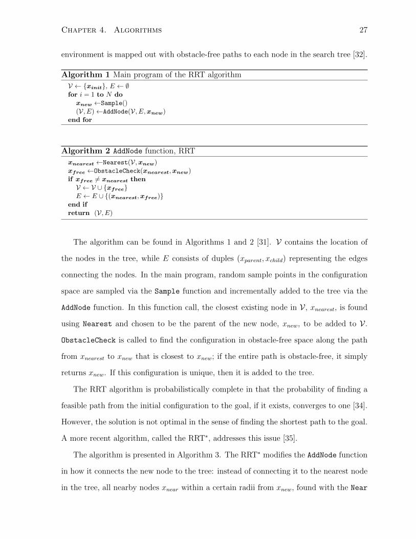
Algorithm 1 Main program of the RRT algorithm
V ← {xinit}, E ← ∅for i = 1 to N do
xnew ←Sample()(V, E)←AddNode(V, E,xnew)
end for
Algorithm 2 AddNode function, RRT
xnearest ←Nearest(V,xnew)xfree ←ObstacleCheck(xnearest,xnew)if xfree 6= xnearest thenV ← V ∪ {xfree}E ← E ∪ {(xnearest,xfree)}
end ifreturn (V, E)
The algorithm can be found in Algorithms 1 and 2 [31]. V contains the location of
the nodes in the tree, while E consists of duples (xparent, xchild) representing the edges
connecting the nodes. In the main program, random sample points in the configuration
space are sampled via the Sample function and incrementally added to the tree via the
AddNode function. In this function call, the closest existing node in V , xnearest, is found
using Nearest and chosen to be the parent of the new node, xnew, to be added to V .
ObstacleCheck is called to find the configuration in obstacle-free space along the path
from xnearest to xnew that is closest to xnew; if the entire path is obstacle-free, it simply
returns xnew. If this configuration is unique, then it is added to the tree.
The RRT algorithm is probabilistically complete in that the probability of finding a
feasible path from the initial configuration to the goal, if it exists, converges to one [34].
However, the solution is not optimal in the sense of finding the shortest path to the goal.
A more recent algorithm, called the RRT∗, addresses this issue [35].
The algorithm is presented in Algorithm 3. The RRT∗ modifies the AddNode function
in how it connects the new node to the tree: instead of connecting it to the nearest node
in the tree, all nearby nodes xnear within a certain radii from xnew, found with the Near
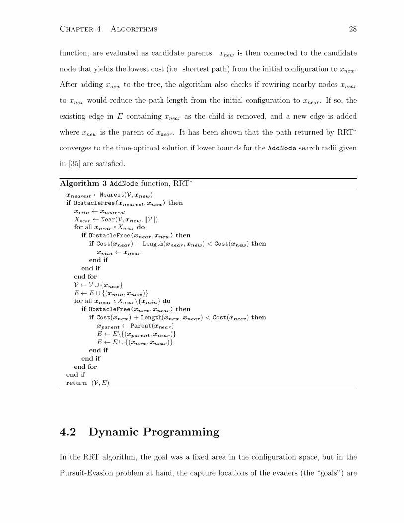
Chapter 4. Algorithms 28
function, are evaluated as candidate parents. xnew is then connected to the candidate
node that yields the lowest cost (i.e. shortest path) from the initial configuration to xnew.
After adding xnew to the tree, the algorithm also checks if rewiring nearby nodes xnear
to xnew would reduce the path length from the initial configuration to xnear. If so, the
existing edge in E containing xnear as the child is removed, and a new edge is added
where xnew is the parent of xnear. It has been shown that the path returned by RRT∗
converges to the time-optimal solution if lower bounds for the AddNode search radii given
in [35] are satisfied.
Algorithm 3 AddNode function, RRT∗
xnearest ←Nearest(V,xnew)if ObstacleFree(xnearest,xnew) then
xmin ← xnearest
Xnear ← Near(V,xnew, ‖V‖)for all xnear ε Xnear do
if ObstacleFree(xnear,xnew) thenif Cost(xnear) + Length(xnear,xnew) < Cost(xnew) then
xmin ← xnear
end ifend if
end forV ← V ∪ {xnew}E ← E ∪ {(xmin,xnew)}for all xnear ε Xnear\{xmin} do
if ObstacleFree(xnew,xnear) thenif Cost(xnew) + Length(xnew,xnear) < Cost(xnear) then
xparent ← Parent(xnear)E ← E\{(xparent,xnear)}E ← E ∪ {(xnew,xnear)}
end ifend if
end forend ifreturn (V, E)
4.2 Dynamic Programming
In the RRT algorithm, the goal was a fixed area in the configuration space, but in the
Pursuit-Evasion problem at hand, the capture locations of the evaders (the “goals”) are
Chapter 4. Algorithms 29
not readily known. Even by assuming that we know the control law of the evaders as
defined in Section 3.2 and that we can predict their trajectories, the continuous setting
of the problem makes it numerically impossible for the RRT to stumble upon these goal
states by just picking random points in space for the pursuer to travel to and hope that
when the pursuer gets there, one of the evaders happens to be there as well. In order
to address this problem, the dynamic programming approach to solving optimization
problems will be used partially in the design of the border patrol algorithm.
Consider the following discrete-time problem: given a set of admissible states S for
the problem, and a set of admissible actions A(s) that depends on the state s ε S the
problem is currently in, there exists instantaneous rewards that are acquired whenever an
action a is taken for a given state s. The value of this reward is represented by r(s, a), and
the objective of the problem is to acquire the greatest sum of rewards possible starting
from any initial state s0 in n time steps. The basic idea of dynamic programming in
solving problems of this type rests on Bellman’s principle of optimality:
Any optimal policy has the property that, whatever the current state and decision, the
remaining decisions must constitute an optimal policy with regard to the state resulting
from the current decision. [39]
Define the value V π(s) as the expected total reward, obtained from the objective
function, of being in s and following a control policy π that defines the actions a taken
for any given state s. If V ∗(s) denotes the value function for the optimal control policy,
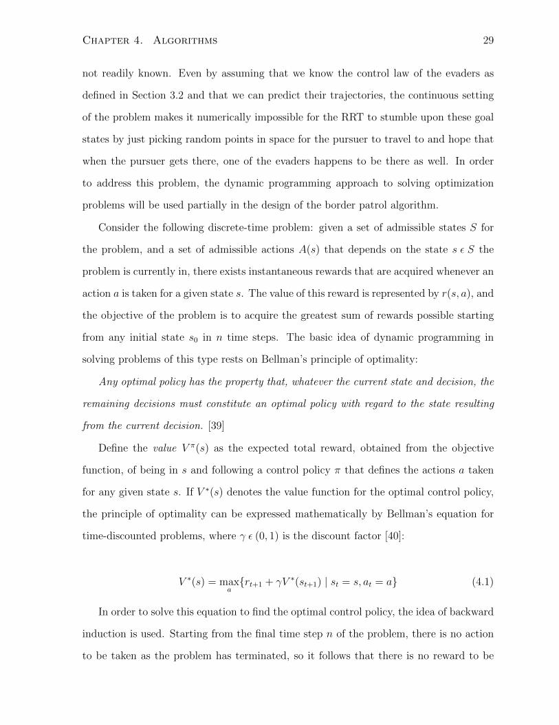
the principle of optimality can be expressed mathematically by Bellman’s equation for
time-discounted problems, where γ ε (0, 1) is the discount factor [40]:
V ∗(s) = maxa{rt+1 + γV ∗(st+1) | st = s, at = a} (4.1)
In order to solve this equation to find the optimal control policy, the idea of backward
induction is used. Starting from the final time step n of the problem, there is no action
to be taken as the problem has terminated, so it follows that there is no reward to be
Chapter 4. Algorithms 30
acquired. Thus, V ∗(sn) = 0 for all s. Then, go back one time step to n−1, and calculate
the optimal value functions V ∗(sn−1) for all possible states s ε S using Eq. 4.1. Repeat
this process of moving back one time step and calculating the value functions for time
t − 1 based on the value functions for t found in the previous iteration, until one has
arrived at t = 0. When this process is complete, the optimal control policy is found for
all s and their corresponding value functions computed.
Although dynamic programming provides a systematic method of finding the opti-
mal control policy, its usefulness in practical applications is limited due to the curse
of dimensionality [40]. As the number of state variables increase, the number of pos-
sible states grows exponentially, and subsequently the number of control policies that
must be evaluated. Furthermore, dynamic programming requires a discrete set of states,
actions, and time steps: using the dynamic programming approach for continuous prob-
lems requires discretizing these sets, and for computational time to be reasonable in the
Pursuit-Evasion problem of interest, the resolution of the discretization mesh would be
too poor for meaningful results.
Still, dynamic programming principles can be borrowed to overcome the issue men-
tioned in the beginning of this section, illustrated in Fig. 4.1. In the research problem
described in Chapter 3, a multi-stage problem is to be solved: for instance, if three
evaders are initially on the loose, the problem would have three stages:
• Stage 1: All three evaders are active, while the pursuer seeks to capture/immobilize
one of them
• Stage 2: One evader has been immobilized, while the remaining two evaders are
active. The pursuer seeks to capture/immobilize one of them
• Stage 3: Two evaders have been immobilized, while the remaining evader is active.
The pursuer seeks to capture/immobilize this last evader
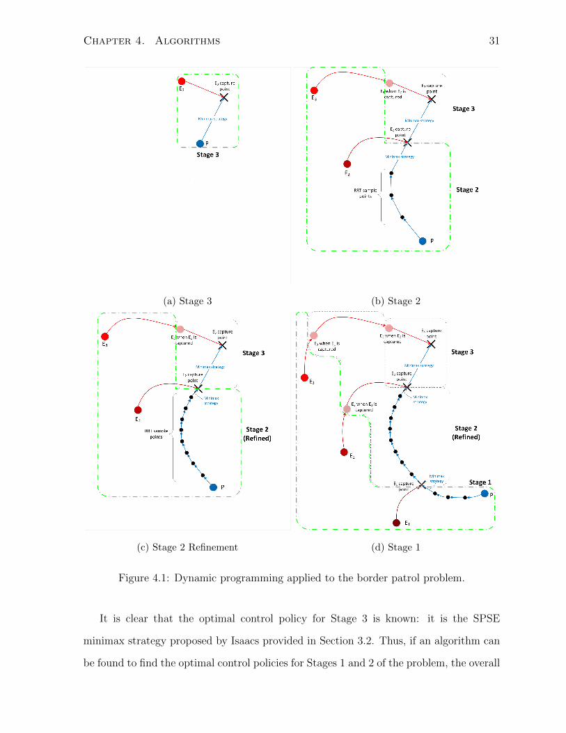
Chapter 4. Algorithms 31
(a) Stage 3 (b) Stage 2
(c) Stage 2 Refinement (d) Stage 1
Figure 4.1: Dynamic programming applied to the border patrol problem.
It is clear that the optimal control policy for Stage 3 is known: it is the SPSE
minimax strategy proposed by Isaacs provided in Section 3.2. Thus, if an algorithm can
be found to find the optimal control policies for Stages 1 and 2 of the problem, the overall

Chapter 4. Algorithms 32
solution to the problem is complete. To find the solution to Stage 2 of the problem, the
RRT algorithm can be used to sample random points and try various trajectories for P
to follow, and once P has completed this trajectory, it switches to the SPSE minimax
strategy to capture the evader (Fig. 4.1b). Although using the SPSE strategy is not
optimal in this case, it is important to provide a policy that captures the evader so that
Stage 2 can be connected to Stage 3. By sampling more points to refine and improve the
trajectory, the length of Stage 2 that relies on the SPSE strategy is reduced (Fig. 4.1c),
and the solution brought closer to optimal. Finally, once Stage 2 is complete, Stage 1
can be carried out in a similar procedure as that of Stage 2 (Fig. 4.1d).
It will be seen that the sampling-based algorithm proposed for border patrol, in
fact, does not follow the backward induction technique by completing Stage n before
commencing Stage n − 1; all stages are sampled and refined simultaneously. What this
illustration demonstrates, however, is that the principle of optimality forms the backbone
of the algorithm developed for this problem. As we already know the minimax optimal
solution for Stage 3, the optimal value function for Stage 3 is known. We then proceed to
estimate the value functions for Stage 2 based on the optimal values for Stage 3 using the
RRT algorithm, and progressively improve them as more samples are taken. At the same
time, the value functions for Stage 1 are estimated based on the value function estimates
for Stage 2. As the number of samples made increases, the value functions approach the
optimal values, and the non-optimal influence of the SPSE minimax strategy used to
connect the different stages gradually dies out.
4.3 RRT Modification for SP2E
When adopting the RRT for use in Pursuit-Evasion problems, several conceptual dif-
ferences first need to be brought to the forefront. In the RRT∗, the accumulated cost
of each node was easily computed as the path length from the starting configuration of

Chapter 4. Algorithms 33
the vehicle to the node. However, in the border patrol scenario, there is no accumulated
cost, as can be seen by simple examination of Eq. 3.13. Since the RRT∗ uses accumulated
cost as the metric for connecting and rewiring nodes in the tree, any suitable algorithm
for the border patrol problem must use a different means to determine how nodes are
connected.
Also, the number of states of the problem has been greatly increased due to the
presence of evaders. Although a natural extension of the RRT would be to include the
states of the evaders in its Sample procedure, this is computationally very expensive:
assuming unicycle dynamics for all players, the state vector size would increase from
2 without evaders to (2 + 2n) for n evaders. Thus, the number of nodes that would
need to be sampled in order to find a feasible trajectory would dramatically increase.
Furthermore, much computational effort would be involved in order to find a control
input for P that would cause the states of the evaders to arrive at the values for the new,
randomly sampled, node. In light of such computational difficulties, the algorithm must
keep the size of the sample space down while retaining information about the states that
are excluded from the sample space.
Algorithm 4 Main program of the SP2E Algorithm
xinit ← [xP,init xE1,init xE2,init]T
V ← {xinit}, E ← ∅for i = 1 to N do
xP,new ←Sample(V)(V, E)←AddNode(V, E,xP,new)
end for
4.3.1 Sampling
The main program of the algorithm developed for the 2-evader border patrol problem
is shown in Algorithm 4 and samples only xP when determining the state x of a new
node. Since the values of xE1 and xE2 are also needed for x, they are computed based
on the edges connecting the new node to the initial configuration (i.e. the root node).

Chapter 4. Algorithms 34
The procedure for computing these states will be explained in 4.3.2.
In order to improve the efficiency of the algorithm, it is desired that the samples,
although random, be more evenly distributed in the sample space. The Sample(V) func-
tion used in Algorithm 4 takes a random sample for xP and checks whether it is at least
a required distance away from the closest node in V . If so, it returns that sample; if
not, it takes a new random sample and continues to do so until it satisfies the minimum
distance requirement.
Algorithm 5 AddNode function, SP2E
xnearest ←Nearest(V,xP,new)(xE1,curr,xE2,curr)←Steer(xnearest,xP,new)xparent ← xnearest
xnew ← [xP,new xE1,curr xE2,curr]T
Xnear ← Near(V,xP,new, ‖V‖)for all xnear ε Xnear do
(xE1,curr,xE2,curr)←Steer(xnear,xP,new)xcurr ← [xP,new xE1,curr xE2,curr]T
if V πS (xcurr) > V πS (xnew) thenxparent ← xnear
xnew ← xcurr
end ifend forV ← V ∪ {xnew}E ← E ∪ {(xparent,xnew)}for all xnear ε Xnear\{xparent} do
(xE1,curr,xE2,curr)←Steer(xnew,xP,near)xcurr ← [xP,near xE1,curr xE2,curr]T
if V πS (xcurr) > V πS (xnear) thenxparent ← Parent(xnear)V ← V\{xnear}E ← E\{(xparent,xnear)}xnear ← xcurr
V ← V ∪ {xnear}E ← E ∪ {(xnew,xnear)}
end ifend forreturn (V, E)
4.3.2 Node Connection
In the AddNode function of the 2-evader border patrol algorithm shown in Algorithm 5,
the general two-phase structure of the RRT∗ algorithm is used: xnew is added to the tree
Chapter 4. Algorithms 35
and connected to the best candidate parent node, and then nearby nodes are rewired
to xnew if it improves their associated costs. When considering different nearby nodes
xnear as parents of xnew, xE1,new and xE2,new will be different depending on which node
is chosen to be the parent. In order to calculate these values, the Steer(xnear,xP,new)
function reads the positions of P , E1, and E2 at xnear, and returns the final positions of
E1 and E2 if P were to travel in a straight line from xP,near to xP,new, and E1 and E2
assumed Isaacs’ control law provided in Section 3.2 for the duration of P ’s travel from
xP,near to xP,new.
4.3.3 Cost Estimate
The metric used for evaluating the benefit of connecting a node to a candidate parent
node is based on the positions of the evaders using the Steer function explained in the
previous section, and the expected reward should P assume a one-by-one SPSE pursuit
policy for the remainder of the problem (as introduced in Section 4.2). Let π1,2(x) be the
pursuit policy where P uses Isaacs’ minimax strategy in Section 3.2 to capture E1, and
once E1 has been immobilized, uses Isaacs’ minimax strategy to capture E2. Similarly,
let π2,1(x) be the pursuit policy where P uses Isaacs’ minimax strategy to capture E2,
and once E2 has been immobilized, uses Isaacs’ minimax strategy to capture E1. Also, let
V π(x) be the value, i.e. the expected total reward obtained from the objective function,
of state x if P follows a policy π. Then, the one-by-one SPSE pursuit policy is
πS(x) = arg maxπ=π1,2,π2,1
V π(x) (4.2)
In Algorithm 5, for each candidate parent node xnear, the Steer function computes
the expected positions of E1 and E2 if P travels from xP,near to xnew, and stores them
in xcurr. Then, the value of xcurr under the policy πS is compared with that of the best
candidate parent found so far. If the value of xcurr is higher than the previous best,
xnear is set as the new best candidate parent, and the positions of E1 and E2 for xnew

Chapter 4. Algorithms 36
updated. This is repeated for all xnear ε Xnear, after which xnew is added to the tree
and connected to the best candidate parent found at the end of this selection process.
4.3.4 Rewiring
When rewiring nearby nodes to xnew, the same Steer function described in Section 4.3.2
is called to determine the positions of E1 and E2 should xnear be rewired to xnew as
its parent. Steer(xnew,xP,near) reads the positions of P , E1, and E2 at xnew, and
returns the final positions of E1 and E2 if P were to travel in a straight line from xP,new
to xP,near, and E1 and E2 assumed Isaacs’ control law provided in Section 3.2 for the
duration of P ’s travel from xP,new to xP,near.
Similarly, the same metric described in Section 4.3.3 is used to determine if setting
xnew as the parent node of xnear would improve the value of xnear. For each nearby
node xnear ε Xnear, after the Steer function computes the expected positions of E1 and
E2 and stores them in xcurr, the value of xcurr under the policy πS is compared with
the existing value of xnear. If it is higher, xnew is set as the new parent of xnear, and
the positions of E1 and E2 for xnear updated.
The class and function definitions in the C++ implementation of the SP2E border
patrol algorithm can be found in Appendix B.
4.4 RRT Modification for SP3E
In the case of 3 evaders, an additional stage is added to the start of the problem where the
pursuer must consider how its actions will influence the movement of all three opponents.
In addition, depending on whether E1, E2, or E3 is captured first during this stage, there
are three possible combinations of remaining evaders still on the loose. Due to this added
complexity, the algorithm developed for this scenario produces a random tree that is a
hybrid of 4 different trees:
Chapter 4. Algorithms 37
• Subtree 0: occurring at the start of the problem when none of the evaders have
been captured yet
• Subtree 1: when E1 has been captured and P needs to capture E2 and E3
• Subtree 2: when E2 has been captured and P needs to capture E1 and E3
• Subtree 3: when E3 has been captured and P needs to capture E1 and E2
Since a third evader is now introduced into the problem, x also includes the state of
E3. Thus, whenever Sample takes random values for xP , the values of xE1 , xE2 , and
xE3 will be computed using Steer.
Furthermore, as the random tree now contains 4 subtrees, each representing a different
scenario of the problem, it is necessary to store that information in x. Let zc be a compact
representation of the mobility of the evaders, i.e. which evaders have been captured. If
evader i is captured, then zc = i. If no evaders have been captured, then zc = 0:
zc =
0 if z1 = z2 = z3 = 1
1 if z1 = 0, z2 = z3 = 1
2 if z2 = 0, z1 = z3 = 1
3 if z3 = 0, z1 = z2 = 1
(4.3)
zc then becomes a state stored in x whose purpose is to represent which subtree each
node belongs to. A node that belongs to subtree i will thus attain zc = i and will be
called a Type i node for the rest of this paper. Note that these 4 combinations of z1, z2,
and z3 are the only combinations that the nodes in the random tree can attain.
The SP3E algorithm is presented in Algorithms 6 to 8. The general structure of the
algorithm remains unchanged, with the AddNode function consisting of a parent selection
phase for xnew followed by a rewiring phase where xnew is considered as a parent for
nearby nodes. The main differences between the SP2E and SP3E algorithms lie in the

Chapter 4. Algorithms 38
Algorithm 6 Main program of the SP3E Algorithm
zc,init ← 0xinit ← [xP,init xE1,init xE2,init xE3,init zc,init]
T
V ← {xinit}, E ← ∅for zc = 1 to 3 do
xspawn ←SpawnNode(xinit, zc)V ← V ∪ {xspawn}E ← E ∪ {(xinit,xspawn)}
end forfor i = 1 to N do
xP,new ←Sample(V)(V, E)←AddNode(V, E,xP,new)
end for
Algorithm 7 AddNode function, SP3E (connection phase)
xnearest ←Nearest(V,xP,new)(xE1,curr,xE2,curr,xE3,curr)←Steer(xnearest,xP,new)
xparent ← xnearest
xnew ← [xP,new xE1,curr xE2,curr
xE3,curr zc,nearest]T
if zc,new = 0 thenzc,spawn ←ChooseType(V)xspawn ←SpawnNode(xnew, zc,spawn)
elsexspawn ← ∅
end ifXnear ←Near(V,xP,new, ‖V‖)for all xnear ε Xnear do
(xE1,curr,xE2,curr,xE3,curr)←Steer(xnear,xP,new)
xcurr ← [xP,new xE1,curr xE2,curr
xE3,curr zc,near]T
if zc,curr = 0 thenzc,spawn,curr ←ChooseType(V)xspawn,curr ←SpawnNode(xcurr, zc,spawn,curr)
elsexspawn,curr ← ∅
end ifif V πS (xcurr) or V πS (xspawn,curr) > V πS (xnew) then
xparent ← xnear
xnew ← xcurr
xspawn ← xspawn.curr
end ifend forV ← V ∪ {xnew}E ← E ∪ {(xparent,xnew)}if xspawn 6= ∅ thenV ← V ∪ {xspawn}E ← E ∪ {(xnew,xspawn)}
end if
Chapter 4. Algorithms 39
Algorithm 8 AddNode function, SP3E (continued - rewiring phase)
Xcheck ← {xnew,xspawn}for all xcheck ε Xcheck doXnear ←Near(V,xP,check, ‖V‖)for all xnear ε Xnear\Ancestor(xcheck) do
if zc,check = zc,near thenVsub ←SubTree(V, E,xnear)(xE1,curr,xE2,curr,xE3,curr)←Steer(xcheck,xP,near)
xcurr ← [xP,near xE1,curr xE2,curr
xE3,curr zc,near]T
V ′sub ←USubTree(V, E,xnear,xcurr)
if max(V πS (x ε V ′sub)) > max(V πS (x ε Vsub)) then
xparent ← Parent(xnear)V ← V\VsubE ← E\{(xparent,xnear)}xnear ← xcurr
V ← V ∪ V ′sub
E ← E ∪ {(xcheck,xnear)}end if
end ifend for
end forreturn (V, E)
hybridization of the subtrees, the way in which cost estimates are used to evaluate node
connections, and the rewiring process. These differences will be explained below.
4.4.1 Tree Hybridization
In order to join the Subtrees 1, 2, and 3 to Subtree 0, it is necessary that the root nodes
of Subtrees 1, 2, and 3 have Type 0 parent nodes. The SpawnNode(x, i) function creates
a Type i node by steering the problem from x to the state where Ei would be captured
if P were to employ Isaacs’ SPSE minimax strategy. This node spawned by SpawnNode
serves as the root node of Subtree i, and is connected to the node x which spawned it.
In the main program (Algorithm 6), this function is called for the Type 0 root node of
the random tree, xinit. In order to start up the algorithm so it contains at least one
node for each subtree, SpawnNode is called three times to create Type 1, 2, and 3 nodes
connected to xinit.
Chapter 4. Algorithms 40
In the AddNode function (Algorithm 7), SpawnNode serves a different purpose. When
a parent node for xnew is found, xnew will assume a value for zc equal to that of xparent
(i.e. if the parent node is Type i, the new node will also be Type i). In order to determine
which candidate parent is best, the values obtained by connecting xnew to the candidate
parent as described in Section 4.3.3 are compared. However, if the candidate parent node
is Type 0, it does not have an associated value V πS , since the policy πS assumes only two
mobile evaders are present, and Type 0 nodes by definition assumes three mobile evaders.
Thus, after Steer is called to drive the state from the candidate parent node to xnew,
SpawnNode is called to create a Type 1, 2, or 3 node that will have an associated value;
the value of this spawn node will then be used to compare with that of other candidate
parent nodes (or their respective spawn nodes). The spawn node type is determined by
the ChooseType function, which randomly picks Type 1, 2, or 3 based on the number of
nodes of each type currently in V :
n1 = ‖V(zc = 1)‖+ ε
n2 = ‖V(zc = 2)‖+ ε
n3 = ‖V(zc = 3)‖+ ε
P (ChooseType = i) =ni
n1 + n2 + n3
, i = 1, 2, 3 (4.4)
Here, ε is a constant value that adjusts the bias towards growing the largest current
subtree. The higher the value of ε, the lower the bias and more even the probability
between the different types. If a Type 0 node is ultimately chosen as the parent of xnew,
the spawn node is also added to V as well as xnew.
4.4.2 Rewiring
The rewiring process described in Algorithm 8 is similar to that in 4.3.4, except that
when a specific rewiring is being evaluated, the values of all descendant nodes affected by

Chapter 4. Algorithms 41
that rewiring are checked. The SubTree(V , E,xnear) function returns the branch Vsub
of V whose root is xnear. Meanwhile, the USubTree(V , E,xnear,xcurr) function also
returns the branch V ′sub of V whose root is xnear, but replaces xnear with xcurr and
updates the states of all its descendant nodes. Thus, whenever rewiring xnear to xnew is
considered, these two functions are called to generate the original and updated branch,
respectively. If the highest value of any node in the updated branch V ′sub is greater than
that of the original branch Vsub, the rewiring is carried out. Note that rewiring is only
considered if xnear and xnew are of the same type.
Chapter 5
Simulations
The algorithms presented in the previous chapter are applied to the formulation given in
Section 3.1.2 for different scenarios. To demonstrate their ability to generate trajectories
that are close to the optimal solution, we compare the results with those generated by
the GPOPS numerical optimal control method [41].
5.1 GPOPS
It is important to find the optimal solution for the control problem presented above
as a benchmark for the online path planning algorithm to be presented in the next
section. This will serve as a proper indicator of how well the algorithm performs. In
this thesis, a numerical method package known as the General Pseudospectral Optimal
Control Software (GPOPS) was used for this purpose. This solver first converts the
optimal control problem into an equivalent nonlinear programming problem and solves
that instead [41]. Although GPOPS is an offline numerical method that requires a good
initial guess of the solution for it to converge and can require several minutes of runtime
to produce the optimal solution, it is used here as a benchmark to compare the border
patrol algorithms to.
GPOPS is an open-source numerical optimal control software that uses the Radau
42
Chapter 5. Simulations 43
Pseudospectral Method [41] and is superior to numerical shooting methods for solv-
ing optimal control problems in terms of radii of convergence [42]. It is a collocation
method that converts the dynamic equations of motion into a system of equations using
time-marching methods, thereby changing the optimal control problem into a nonlinear
programming problem of the form
min J(q) (5.1)
subject to
g(q) = 0 (5.2)
where, if xi and ui are the state and control at different times ti and tM = tf , then
q = (x0,x1, ...,xM ,u0,u1, ...,uM−1)
The constraints in Eq. (5.2) include the system of equations resulting from the dis-
cretization of the dynamic equations of motion, and the terminal constraints ψ [42]. In
GPOPS, the collocation points are the Legendre-Gauss-Radau points and uses Gaussian
quadrature to approximate the integrals in the problem [41]. The software also checks
whether the optimality conditions of the equivalent optimal control problem are indeed
satisfied by the generated numerical solution.
Because the evaders have a switching control law as indicated by Eq. (3.36), a sigmoid
function was used to remove the discontinuity at the point where the evader’s control
input switches for the purpose of allowing GPOPS to converge to a solution:
p (±, xEi, yEi
) =1
1 + e±ζ
[vPvE·((xEi
−xD)2+(yEi−yD)2)−(xP−xD)2+(yP−yD)2
] (5.3)
where ζ is the sigmoid sharpness parameter. The higher the value of ζ, the more the
sigmoid function resembles a step function. In other words, increasing the sharpness
Chapter 5. Simulations 44
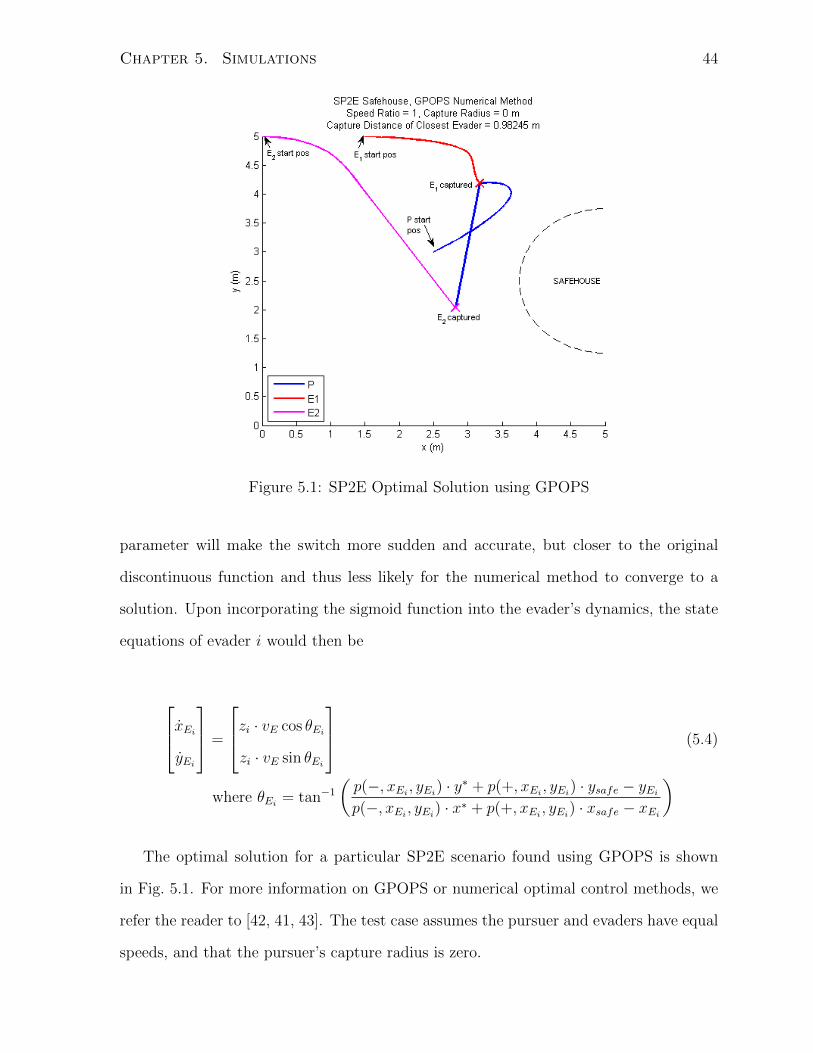
Figure 5.1: SP2E Optimal Solution using GPOPS
parameter will make the switch more sudden and accurate, but closer to the original
discontinuous function and thus less likely for the numerical method to converge to a
solution. Upon incorporating the sigmoid function into the evader’s dynamics, the state
equations of evader i would then be
xEi
yEi
=
zi · vE cos θEi
zi · vE sin θEi
(5.4)
where θEi= tan−1
(p(−, xEi
, yEi) · y∗ + p(+, xEi
, yEi) · ysafe − yEi
p(−, xEi, yEi
) · x∗ + p(+, xEi, yEi
) · xsafe − xEi
)
The optimal solution for a particular SP2E scenario found using GPOPS is shown
in Fig. 5.1. For more information on GPOPS or numerical optimal control methods, we
refer the reader to [42, 41, 43]. The test case assumes the pursuer and evaders have equal
speeds, and that the pursuer’s capture radius is zero.
Chapter 5. Simulations 45
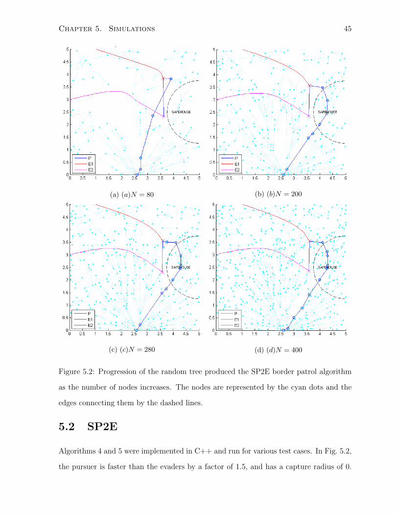
(a) (a)N = 80 (b) (b)N = 200
(c) (c)N = 280 (d) (d)N = 400
Figure 5.2: Progression of the random tree produced the SP2E border patrol algorithm
as the number of nodes increases. The nodes are represented by the cyan dots and the
edges connecting them by the dashed lines.
5.2 SP2E
Algorithms 4 and 5 were implemented in C++ and run for various test cases. In Fig. 5.2,
the pursuer is faster than the evaders by a factor of 1.5, and has a capture radius of 0.
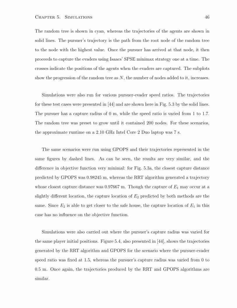
Chapter 5. Simulations 46
The random tree is shown in cyan, whereas the trajectories of the agents are shown in
solid lines. The pursuer’s trajectory is the path from the root node of the random tree
to the node with the highest value. Once the pursuer has arrived at that node, it then
proceeds to capture the evaders using Isaacs’ SPSE minimax strategy one at a time. The
crosses indicate the positions of the agents when the evaders are captured. The subplots
show the progression of the random tree as N , the number of nodes added to it, increases.
Simulations were also run for various pursuer-evader speed ratios. The trajectories
for these test cases were presented in [44] and are shown here in Fig. 5.3 by the solid lines.
The pursuer has a capture radius of 0 m, while the speed ratio is varied from 1 to 1.7.
The random tree was preset to grow until it contained 200 nodes. For these scenarios,
the approximate runtime on a 2.10 GHz Intel Core 2 Duo laptop was 7 s.
The same scenarios were run using GPOPS and their trajectories represented in the
same figures by dashed lines. As can be seen, the results are very similar, and the
difference in objective function very minimal: for Fig. 5.3a, the closest capture distance
predicted by GPOPS was 0.98245 m, whereas the RRT algorithm generated a trajectory
whose closest capture distance was 0.97667 m. Though the capture of E1 may occur at a
slightly different location, the capture location of E2 predicted by both methods are the
same. Since E2 is able to get closer to the safe house, the capture location of E1 in this
case has no influence on the objective function.
Simulations were also carried out where the pursuer’s capture radius was varied for
the same player initial positions. Figure 5.4, also presented in [44], shows the trajectories
generated by the RRT algorithm and GPOPS for the scenario where the pursuer-evader
speed ratio was fixed at 1.5, whereas the pursuer’s capture radius was varied from 0 to
0.5 m. Once again, the trajectories produced by the RRT and GPOPS algorithms are
similar.

Chapter 5. Simulations 47
(a) (a)vP /vE = 1 (b) (b)vP /vE = 1.4
(c) (c)vP /vE = 1.5 (d) (d)vP /vE = 1.7
Figure 5.3: Trajectories generated by the SP2E border patrol algorithm (solid lines) and
the GPOPS numerical method (dashed lines) for different speed ratios. The random tree
produced by the RRT algorithm was grown until it contained 200 nodes.
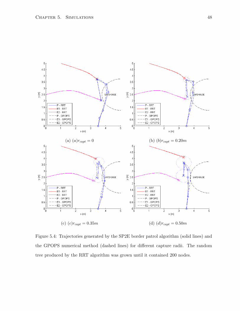
Chapter 5. Simulations 48
(a) (a)rcapt = 0 (b) (b)rcapt = 0.20m
(c) (c)rcapt = 0.35m (d) (d)rcapt = 0.50m
Figure 5.4: Trajectories generated by the SP2E border patrol algorithm (solid lines) and
the GPOPS numerical method (dashed lines) for different capture radii. The random
tree produced by the RRT algorithm was grown until it contained 200 nodes.
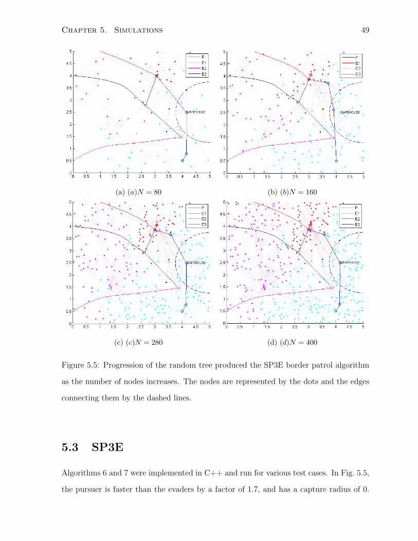
Chapter 5. Simulations 49
(a) (a)N = 80 (b) (b)N = 160
(c) (c)N = 280 (d) (d)N = 400
Figure 5.5: Progression of the random tree produced the SP3E border patrol algorithm
as the number of nodes increases. The nodes are represented by the dots and the edges
connecting them by the dashed lines.
5.3 SP3E
Algorithms 6 and 7 were implemented in C++ and run for various test cases. In Fig. 5.5,
the pursuer is faster than the evaders by a factor of 1.7, and has a capture radius of 0.

Chapter 5. Simulations 50
The random tree is shown in various colours: nodes belonging to Subtree 0 are shown in
cyan, Subtree 1 in red, Subtree 2 in magenta, and Subtree 3 in black. As was the case in
SP2E, the pursuer’s trajectory is the path from the root node of the random tree to the
node with the highest value. Once the pursuer has arrived at that node, it then proceeds
to capture the remaining two evaders using Isaacs’ SPSE minimax strategy one at a time.
The crosses indicate the positions of the agents when the evaders are captured.
Simulations were also run for various pursuer-evader speed ratios and the resulting
trajectories shown in Fig. 5.6 by the solid lines. The pursuer has a capture radius of 0
m, while the speed ratio is varied from 1.5 to 2.0. The random tree was preset to grow
until it contained 200 nodes. For these scenarios, the approximate runtime on a 2.10
GHz Intel Core 2 Duo laptop was 12 s.
The same scenarios were run using GPOPS and their trajectories represented by
dashed lines. Again, the results are very similar, and the difference in objective function
very minimal. In fact, in Fig. 5.6b, the border patrol algorithm actually outperforms
the trejectory generated by GPOPS: the closest capture distance predicted by GPOPS
was 0.31391 m, whereas the RRT algorithm generated a trajectory whose closest capture
distance was 0.55008 m. In this case, it is likely that GPOPS is stuck in a local maxima,
while the RRT algorithm presented in this paper has the ability to overcome such ob-
stacles due to its sample-based design. For the other scenarios presented in Fig. 5.6, the
proximity of the closest capture location from the safe house found by the border patrol
algorithm and GPOPS are very similar.
Simulations were also carried out where the pursuer’s capture radius was varied for
the same player initial positions. Fig. 5.7 shows the trajectories generated by the RRT
algorithm and GPOPS for the scenario where the pursuer-evader speed ratio was fixed
at 1.6, while the pursuer’s capture radius was varied from 0 to 0.6 m. Once again, the
trajectories produced by the RRT and GPOPS algorithms are similar.
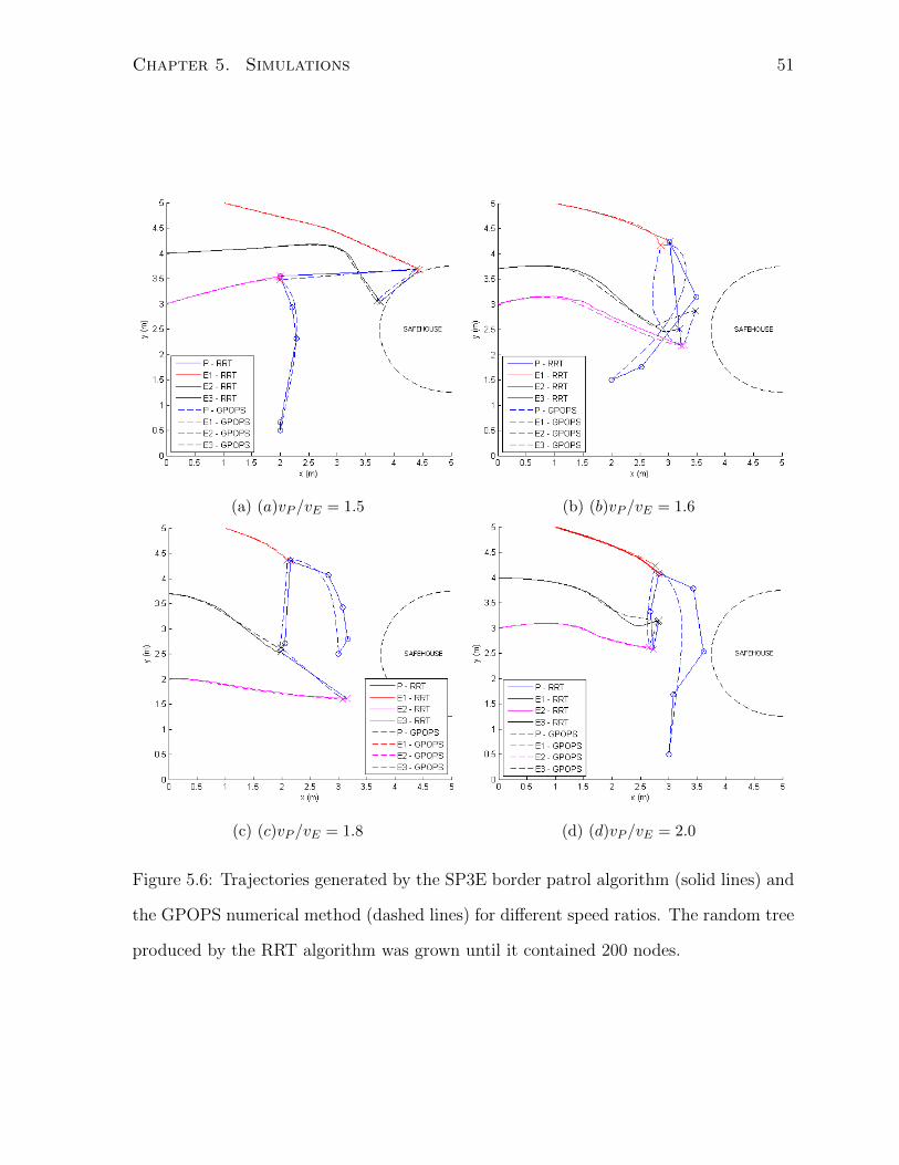
Chapter 5. Simulations 51
(a) (a)vP /vE = 1.5 (b) (b)vP /vE = 1.6
(c) (c)vP /vE = 1.8 (d) (d)vP /vE = 2.0
Figure 5.6: Trajectories generated by the SP3E border patrol algorithm (solid lines) and
the GPOPS numerical method (dashed lines) for different speed ratios. The random tree
produced by the RRT algorithm was grown until it contained 200 nodes.
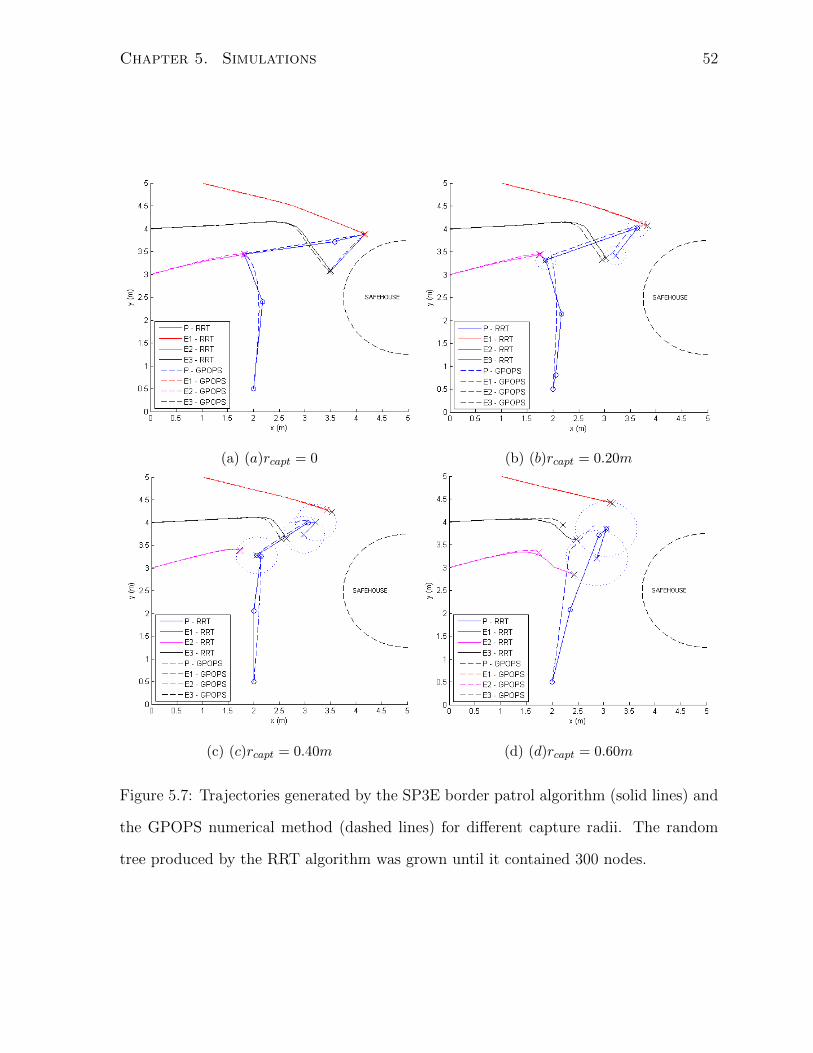
Chapter 5. Simulations 52
(a) (a)rcapt = 0 (b) (b)rcapt = 0.20m
(c) (c)rcapt = 0.40m (d) (d)rcapt = 0.60m
Figure 5.7: Trajectories generated by the SP3E border patrol algorithm (solid lines) and
the GPOPS numerical method (dashed lines) for different capture radii. The random
tree produced by the RRT algorithm was grown until it contained 300 nodes.
Chapter 6
Experiments
To demonstrate the feasibility of using the border patrol algorithms developed earlier for
physical applications, experiments were conducted on ground robots for both the two and
three-evader scenarios. By developing a suitable closed-loop control law for the pursuer
to follow the trajectory produced by the algorithm, and by incorporating feedback of the
evaders’ positions, a complete picture of the border patrol pursuit system is provided
that can capture border trespassers before they arrive at the safe house.
6.1 Setup
The experimental setup consists of four iRobot Creates, shown in Fig. 6.1, three acting
as the evaders and one as the pursuer. The four robots are identical and acquire their
poses from a 10-camera Vicon motion capture system mounted at the perimeter of the
test facility. The experimental scenario is set up as defined in 3.1.2, with lb = 5m and
rsafe = 1.25m. The evader robots begin at Xenter, the left-half perimeter of X, while the
pursuer is allowed to begin at any point in X. Once the problem begins, the pursuer
robot must compute a trajectory to follow so it can capture all evaders before they arrive
at Xsafe. An evader is assumed to be captured if it is within the pursuer’s capture region
Xcapt.
53
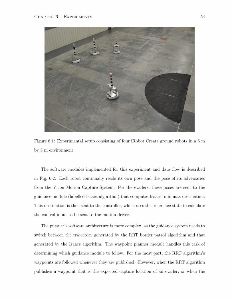
Chapter 6. Experiments 54
Figure 6.1: Experimental setup consisting of four iRobot Create ground robots in a 5 m
by 5 m environment
The software modules implemented for this experiment and data flow is described
in Fig. 6.2. Each robot continually reads its own pose and the pose of its adversaries
from the Vicon Motion Capture System. For the evaders, these poses are sent to the
guidance module (labelled Isaacs algorithm) that computes Isaacs’ minimax destination.
This destination is then sent to the controller, which uses this reference state to calculate
the control input to be sent to the motion driver.
The pursuer’s software architecture is more complex, as the guidance system needs to
switch between the trajectory generated by the RRT border patrol algorithm and that
generated by the Isaacs algorithm. The waypoint planner module handles this task of
determining which guidance module to follow. For the most part, the RRT algorithm’s
waypoints are followed whenever they are published. However, when the RRT algorithm
publishes a waypoint that is the expected capture location of an evader, or when the

Chapter 6. Experiments 55
pursuer has completed all waypoints published by the RRT algorithm, the waypoint
planner hands control over to the Isaacs algorithm module for the purpose of capturing
a specific evader.
Figure 6.2: Experimental setup data flow
6.2 Controller Design
The waypoints provide the controller module with reference states that the robot needs to
arrive at sequentially before moving on to the next waypoint. Given an inertial reference
frame FV whose coordinates are given by the Vicon Motion Capture System and a goal
state xg = [xg yg θg]T , the control law developed to drive the robot to this state is based
on the motion controller proposed in [45]. Assume a robot reference frame FR whose
origin is pinned to the robot center of mass and whose x-axis points in the direction of
Chapter 6. Experiments 56
the robot heading θV , as shown in Fig. 6.3. As the RRT algorithm only provides the x
and y coordinates of the goal state xg, the desired final heading θg is specified to be the
angle between the vector from the initial position of the robot to the goal state and the
x-axis of FV . Also assume a goal inertial frame FG translated and rotated with respect
to FV by (xr, yr) and θg. The pose error vector in FR is given by
e =
[x y θ
]T(6.1)
As the control inputs to the robot are its forward and angular speeds v and ω, the task,
then, is to find a controller of the form
v(t)
ω(t)
= K · e =
k11 k12 k13
k21 k22 k23
e, kij = k(t, e) (6.2)
such that the pose error vector e goes to zero in finite time [45].
The kinematics of the robot in the goal inertial frame is given by
x
y
θ
=
cos θ 0
sin θ 0
0 1
vω
(6.3)
Let r be the vector from the position of the robot to the goal state, and α be the
angle between r and the x-axis of FR. Perform a coordinate transformation into polar
coordinates in FG:
ρ =√
∆x2 + ∆y2 (6.4)
α = atan2(∆y,∆x)− θ (6.5)
β = −θ − α (6.6)
where ρ is the distance between the robot and the goal and β is the angle between r and
the x-axis of FG. The kinematics expressed in these coordinates is

Chapter 6. Experiments 57
Figure 6.3: Robot kinematics
ρ
α
β
=
− cosα 0
sinαρ
−1
− sinαρ
0
vω
(6.7)
The proposed control law takes the form
vω
=
kρ 0 0
0 kα kβ
ρ
α
β
(6.8)
For this application, as we constrain the vehicles to travel at constant speeds, we set
kρ = kcρ/ρ, where kcρ is constant. The resulting closed loop system has been shown in
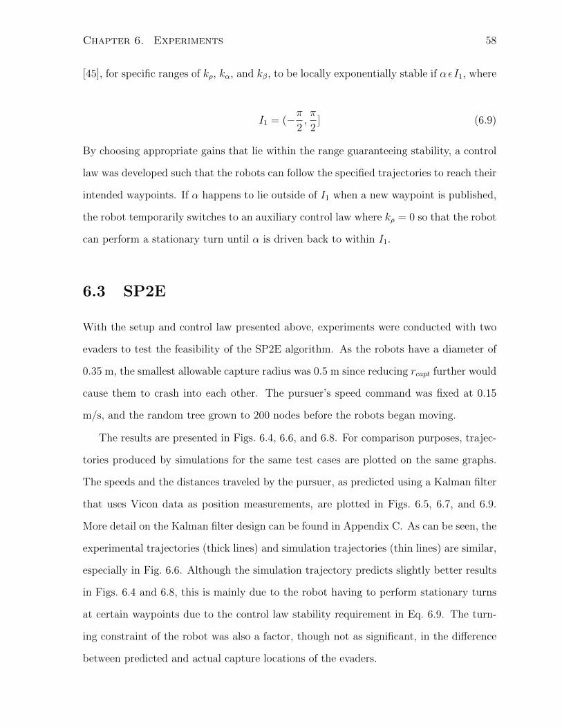
Chapter 6. Experiments 58
[45], for specific ranges of kρ, kα, and kβ, to be locally exponentially stable if αεI1, where
I1 = (−π2,π
2] (6.9)
By choosing appropriate gains that lie within the range guaranteeing stability, a control
law was developed such that the robots can follow the specified trajectories to reach their
intended waypoints. If α happens to lie outside of I1 when a new waypoint is published,
the robot temporarily switches to an auxiliary control law where kρ = 0 so that the robot
can perform a stationary turn until α is driven back to within I1.
6.3 SP2E
With the setup and control law presented above, experiments were conducted with two
evaders to test the feasibility of the SP2E algorithm. As the robots have a diameter of
0.35 m, the smallest allowable capture radius was 0.5 m since reducing rcapt further would
cause them to crash into each other. The pursuer’s speed command was fixed at 0.15
m/s, and the random tree grown to 200 nodes before the robots began moving.
The results are presented in Figs. 6.4, 6.6, and 6.8. For comparison purposes, trajec-
tories produced by simulations for the same test cases are plotted on the same graphs.
The speeds and the distances traveled by the pursuer, as predicted using a Kalman filter
that uses Vicon data as position measurements, are plotted in Figs. 6.5, 6.7, and 6.9.
More detail on the Kalman filter design can be found in Appendix C. As can be seen, the
experimental trajectories (thick lines) and simulation trajectories (thin lines) are similar,
especially in Fig. 6.6. Although the simulation trajectory predicts slightly better results
in Figs. 6.4 and 6.8, this is mainly due to the robot having to perform stationary turns
at certain waypoints due to the control law stability requirement in Eq. 6.9. The turn-
ing constraint of the robot was also a factor, though not as significant, in the difference
between predicted and actual capture locations of the evaders.
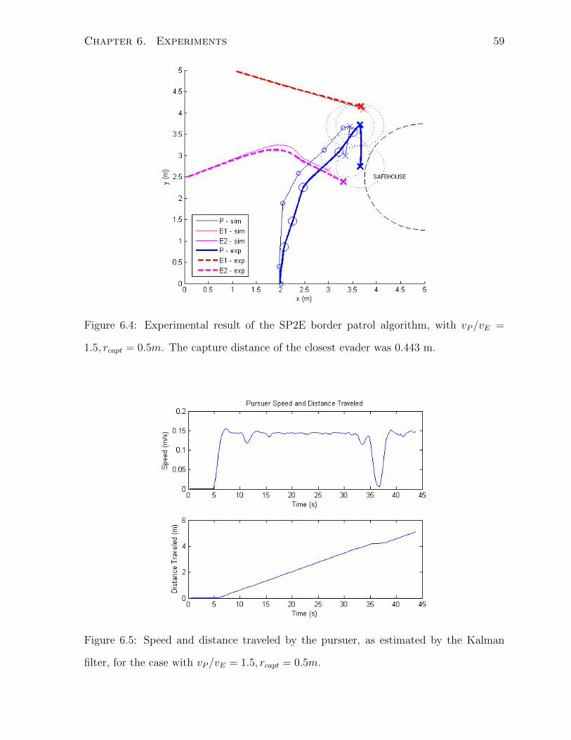
Chapter 6. Experiments 59
Figure 6.4: Experimental result of the SP2E border patrol algorithm, with vP/vE =
1.5, rcapt = 0.5m. The capture distance of the closest evader was 0.443 m.
Figure 6.5: Speed and distance traveled by the pursuer, as estimated by the Kalman
filter, for the case with vP/vE = 1.5, rcapt = 0.5m.
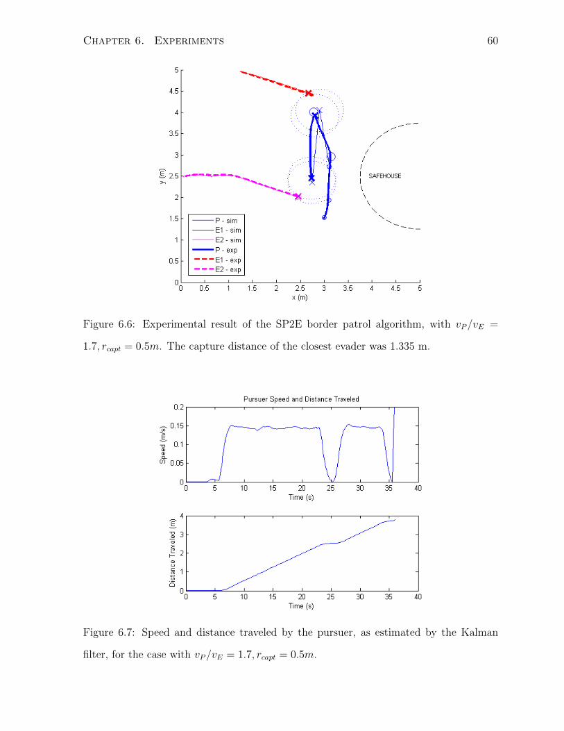
Chapter 6. Experiments 60
Figure 6.6: Experimental result of the SP2E border patrol algorithm, with vP/vE =
1.7, rcapt = 0.5m. The capture distance of the closest evader was 1.335 m.
Figure 6.7: Speed and distance traveled by the pursuer, as estimated by the Kalman
filter, for the case with vP/vE = 1.7, rcapt = 0.5m.
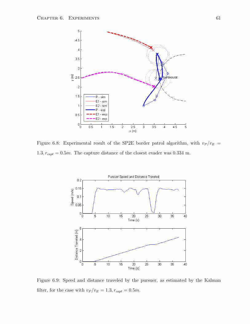
Chapter 6. Experiments 61
Figure 6.8: Experimental result of the SP2E border patrol algorithm, with vP/vE =
1.3, rcapt = 0.5m. The capture distance of the closest evader was 0.334 m.
Figure 6.9: Speed and distance traveled by the pursuer, as estimated by the Kalman
filter, for the case with vP/vE = 1.3, rcapt = 0.5m.
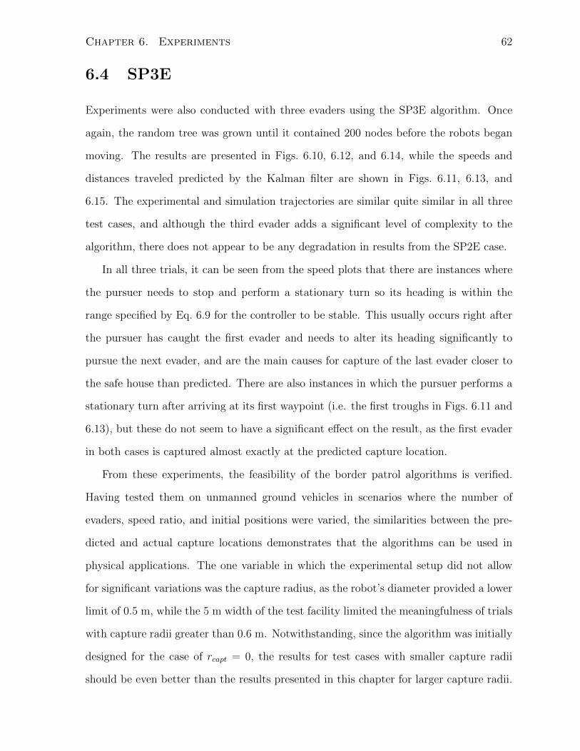
Chapter 6. Experiments 62
6.4 SP3E
Experiments were also conducted with three evaders using the SP3E algorithm. Once
again, the random tree was grown until it contained 200 nodes before the robots began
moving. The results are presented in Figs. 6.10, 6.12, and 6.14, while the speeds and
distances traveled predicted by the Kalman filter are shown in Figs. 6.11, 6.13, and
6.15. The experimental and simulation trajectories are similar quite similar in all three
test cases, and although the third evader adds a significant level of complexity to the
algorithm, there does not appear to be any degradation in results from the SP2E case.
In all three trials, it can be seen from the speed plots that there are instances where
the pursuer needs to stop and perform a stationary turn so its heading is within the
range specified by Eq. 6.9 for the controller to be stable. This usually occurs right after
the pursuer has caught the first evader and needs to alter its heading significantly to
pursue the next evader, and are the main causes for capture of the last evader closer to
the safe house than predicted. There are also instances in which the pursuer performs a
stationary turn after arriving at its first waypoint (i.e. the first troughs in Figs. 6.11 and
6.13), but these do not seem to have a significant effect on the result, as the first evader
in both cases is captured almost exactly at the predicted capture location.
From these experiments, the feasibility of the border patrol algorithms is verified.
Having tested them on unmanned ground vehicles in scenarios where the number of
evaders, speed ratio, and initial positions were varied, the similarities between the pre-
dicted and actual capture locations demonstrates that the algorithms can be used in
physical applications. The one variable in which the experimental setup did not allow
for significant variations was the capture radius, as the robot’s diameter provided a lower
limit of 0.5 m, while the 5 m width of the test facility limited the meaningfulness of trials
with capture radii greater than 0.6 m. Notwithstanding, since the algorithm was initially
designed for the case of rcapt = 0, the results for test cases with smaller capture radii
should be even better than the results presented in this chapter for larger capture radii.
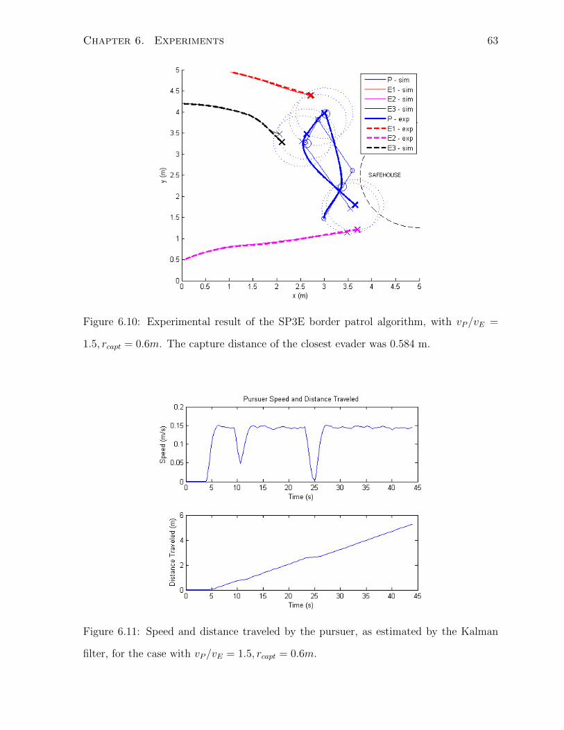
Chapter 6. Experiments 63
Figure 6.10: Experimental result of the SP3E border patrol algorithm, with vP/vE =
1.5, rcapt = 0.6m. The capture distance of the closest evader was 0.584 m.
Figure 6.11: Speed and distance traveled by the pursuer, as estimated by the Kalman
filter, for the case with vP/vE = 1.5, rcapt = 0.6m.
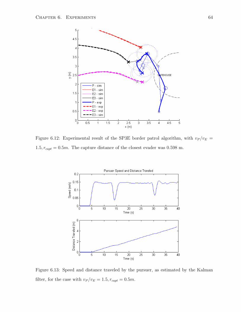
Chapter 6. Experiments 64
Figure 6.12: Experimental result of the SP3E border patrol algorithm, with vP/vE =
1.5, rcapt = 0.5m. The capture distance of the closest evader was 0.598 m.
Figure 6.13: Speed and distance traveled by the pursuer, as estimated by the Kalman
filter, for the case with vP/vE = 1.5, rcapt = 0.5m.
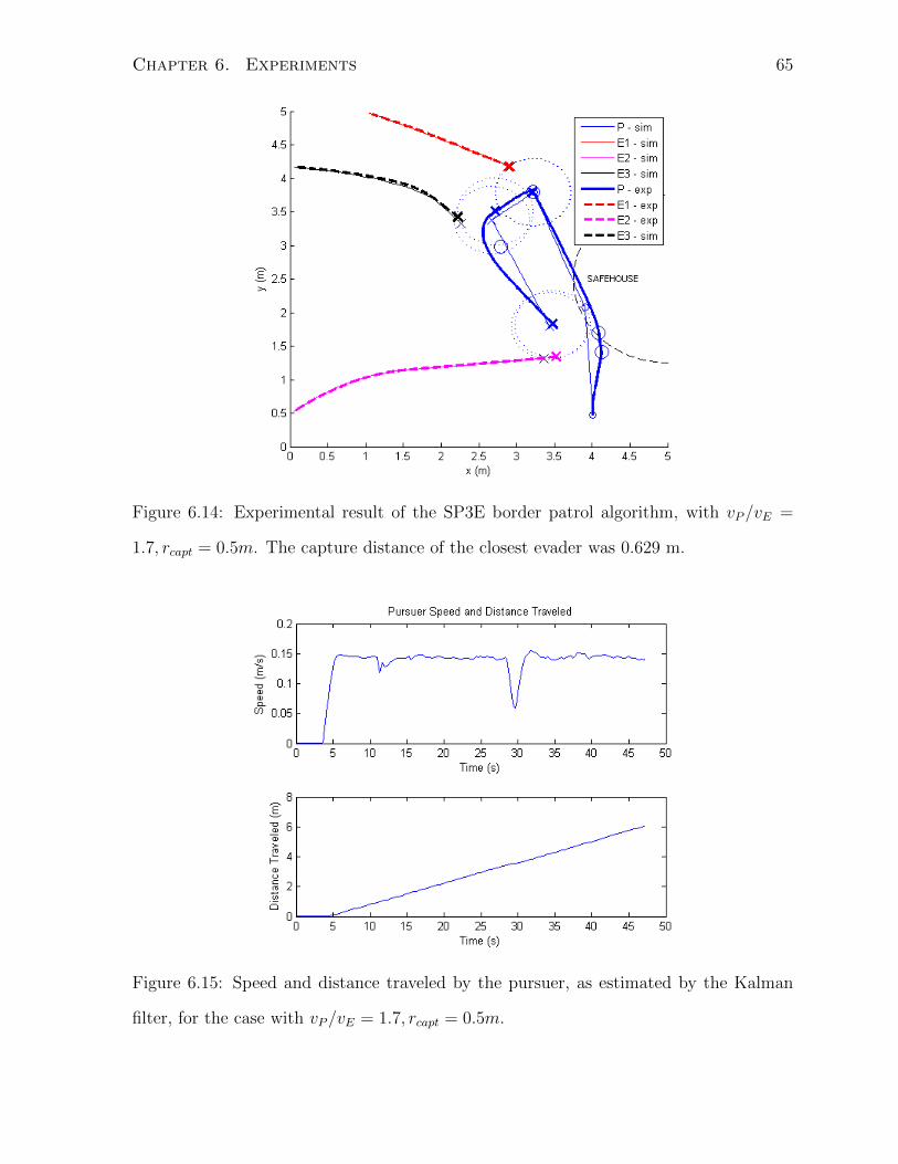
Chapter 6. Experiments 65
Figure 6.14: Experimental result of the SP3E border patrol algorithm, with vP/vE =
1.7, rcapt = 0.5m. The capture distance of the closest evader was 0.629 m.
Figure 6.15: Speed and distance traveled by the pursuer, as estimated by the Kalman
filter, for the case with vP/vE = 1.7, rcapt = 0.5m.
Chapter 7
Conclusion
7.1 Contribution
In this thesis, an efficient sampling-based algorithm was presented for the border pa-
trol Pursuit-Evasion game, where a single vehicle was responsible for capturing multiple
trespassers before they found refuge in a target safe house. An appropriate model of
the evaders’ control law was first developed based on Isaacs’ Target Guarding problem,
extended to the case where the pursuer is faster than the evader, and demonstrated to be
the minimax solution in the SPSE case. Using this model, an algorithm was developed
for the resulting optimal control problem based on the Rapidly-exploring Random Tree
path planning algorithm and concepts from Dynamic Programming. Separate algorithms
were developed for the case of two and three evaders.
Simulations were run for different scenarios, including two and three evaders with
varying speed ratios, capture radii, and initial positions. By comparing the results with
the solution generated by the GPOPS numerical optimal control method, it was shown
that the trajectories produced by the algorithm were near-optimal and efficient in quickly
generating the solution. Experiments were also carried out to demonstrate the feasibility
of implementing this path planning algorithm on physical applications. A closed-loop
66

Chapter 7. Conclusion 67
feedback system was set up for the ground robots to capture evaders and a control
law developed for following the trajectory produced by the border patrol algorithm.
Experimental results showed that the final trajectories followed by the robot were similar
to that predicted in simulation.
7.2 Future Work
Future work on these algorithms includes considering the holonomic constraints of the
robot into the algorithms for the purpose of generating trajectories that can be more
accurately followed by the vehicle. A possible method for including such holonomic
constraints, such as the minimum turning radius, is to include the heading angle of the
pursuer in the algorithm’s sampling procedure, and connect nodes within the random
tree using Dubins’ paths, which were shown in [46] to be optimal in terms of path length,
and the choice of the six different Dubins’ paths classified for different scenarios in [47].
The addition of the heading angle during sampling increases the dimensionality of the
configuration space, so improvements in computational efficiency will be necessary for
the non-holonomic version of the algorithm to be efficient enough for real-time guidance
systems.
In addition, proving the algorithm’s convergence to the optimal solution as the number
of nodes in the tree increases and feasibility studies on the region in which the pursuer
is able to catch all evaders are theoretical tasks that would provide a more complete
picture of the border patrol problem. Also, while the algorithm is able to generate near-
optimal trajectories within several seconds, improvements can be made in improving its
computational efficiency. Such improvements would allow for expanding the algorithm
such that it continually improves the trajectory even as the robot is moving.
Appendix A
SPSE Target Guarding
State equations for the SPSE problem:
xP = vP cos θP yP = vP sin θP
xE = vE cos θE yE = vE sin θE
Objective function:
J = φ(xf ) +
∫ tf
0
L(x, uP , uE)dt, L(x, uP , uE) = 0
=√
(xE,f − xD)2 + (yE,f − yD)2 − rD
Terminal conditions:
ψ =√
(xE − xP )2 + (yE − yP )2 − rcapt = 0
Modified space:
x1 = xE − xP x2 = yE − yP
x3 = xD − xE x4 = yD − yE
The problem, in the modified space, is then
x1 = vE cos θE − vP cos θP x2 = vE sin θE − vP sin θP
x3 = −vE cos θE x4 = −vE sin θE
68
Appendix A. SPSE Target Guarding 69
J =√x23,f + x24,f − rD (A.1)
ψ =√x21 + x22 − rcapt = 0 (A.2)
Isaacs’ Main Equation:
H∗(xf , uP,f , uE,f , λf ) = 0
−vP (λ1 cos θ∗P + λ2 sin θ∗P )− vE((−λ1 + λ2) cos θ∗E + (−λ2 + λ4) sin θ∗E) = 0 (A.3)
From [1],
maxθP
(λ1 cos θP + λ2 sin θP ) = ρ1 where
ρ1 =√λ21 + λ22, cos θ∗P =
λ1ρ1, sin θ∗P =
λ2ρ1
and
minθE
((−λ1 + λ3) cos θE + (−λ2 + λ4) sin θE) = −ρ2 where
ρ2 =√
(−λ1 + λ3)2 + (−λ2 + λ4)2, cos θ∗E =−(−λ1 + λ3)
ρ1, sin θ∗E =
−(−λ2 + λ4)
ρ1
Eq. A.3 then becomes
−vPρ1 + vEρ2 = 0 (A.4)
The costate equations, from Eq. 3.32, are:
λ1 = λ2 = λ3 = λ4 = 0 (A.5)
Parametric terminal surface:
x1 = rcapt cos s1 x2 = rcapt sin s1
x3 = s2 x4 = s3
Appendix A. SPSE Target Guarding 70
From Eq. 3.34, the following end-point conditions are:
∂φ
∂s1= 0 = λ1(−rcapt sin s1) + λ2(rcapt cos s1) → λ2 = λ1 tan s1 (A.6)
∂φ
∂s2=
s2√s22 + s23
= λ3 (A.7)
∂φ
∂s3=
s3√s22 + s23
= λ4 (A.8)
Also, from Eq. A.4,
−vP√λ21 + λ22 + vE
√(−λ1 + λ3)2 + (−λ2 + λ4)2 = 0 (A.9)
Sub Eqs. A.6, A.7, A.8 in A.9:(((vPvE
)2
− 1
)sec2 s1
)λ21 + 2
(s2 + s3 tan s1√
s22 + s23
)λ1 − 1 = 0 (A.10)
This quadratic equation can be solved for an explicit expression of λ1, while Eqs. A.6,
A.7, and A.8 provide expressions for λ2, λ3, and λ4.
Backward integration: τ = tf − t, u = dudτ
x1 = vP cos θP − vE cos θE x2 = vP sin θP − vE sin θE
x3 = vE cos θE x4 = vE sin θE
Since λ’s are constant, trajectories are all straight lines emanating from the capture point.
Integration yields the following minimax trajectory:
x1 =
[vP
(λ1ρ1
)+ vE
(λ3 − λ1ρ2
)]τ + rcapt cos s1 (A.11)
x2 =
[vP
(λ2ρ1
)+ vE
(λ4 − λ2ρ2
)]τ + rcapt sin s1 (A.12)
x3 =
[−vE
(λ3 − λ1ρ2
)]τ + s2 (A.13)
x4 =
[−vE
(λ4 − λ2ρ2
)]τ + s3 (A.14)

Appendix B
C++ SP2E Algorithm
Node.h
#ifndef NODE_H
#define NODE_H
#include <vector>
#include "fn_header.h"
using namespace std;
class Node {
public:
int id; // this is only for MATLAB plotting purposes
double x, y;
double payoff;
double xe1,ye1,xe2,ye2;
vector<Node *> children;
Node * parent;
Node(double,double,Node *,int);
~Node();
void set_Epos(double,double,double,double);
void set_payoff(double);
void add_child(Node *);
void change_parent(Node *);
void steer(double,double,double &, double &, double &, double &);
vector<Node *> ancestors();
void update_descendants();
};
//--------------------------------------------------------------------------------
// Constructor
Node::Node(double x_in, double y_in, Node * parent_in, int id_in) {
x = x_in;
71

Appendix B. C++ SP2E Algorithm 72
y = y_in;
parent = parent_in; // if parent == 0, it is a null pointer and thus indicates a root node
id = id_in;
// if node has a parent, add node to parent’s list to children
if (parent != 0) parent->add_child(this);
}
//--------------------------------------------------------------------------------
// Destructor
Node::~Node() {
delete parent;
}
//--------------------------------------------------------------------------------
// set E1 and E2’s positions if P is at this node
void Node::set_Epos(double xe1_in, double ye1_in, double xe2_in, double ye2_in) {
xe1 = xe1_in;
ye1 = ye1_in;
xe2 = xe2_in;
ye2 = ye2_in;
}
//--------------------------------------------------------------------------------
// set payoff of node
void Node::set_payoff(double payoff_in) {
payoff = payoff_in;
}
//--------------------------------------------------------------------------------
// add child
void Node::add_child(Node * child_in) {
children.push_back(child_in);
}
//--------------------------------------------------------------------------------
// change parent
void Node::change_parent(Node * parent_in) {
// erase this node as a child of old parent
Node * old_parent = parent;
for (int i=0; i < (int) old_parent->children.size(); i++) {
if (old_parent->children[i] == this) {
old_parent->children.erase(old_parent->children.begin()+i);
break;
}
}
// change parent from old to new
parent = parent_in;
// add this node as a child of the new parent
parent->children.push_back(this);
}
//--------------------------------------------------------------------------------
Appendix B. C++ SP2E Algorithm 73
// calculate E1 and E2’s coords if P went from current node to specified coords
void Node::steer(double x_f, double y_f, double &xe1_f, double &ye1_f, double &xe2_f, double &ye2_f) {
double xp_curr, yp_curr, xe1_curr, ye1_curr, xe2_curr, ye2_curr;
double theta_p, theta_e1, theta_e2, payoff1_min, payoff2_min;
double length, t_capt, n_raw, dt_use, dl_use;
int n_use;
xp_curr = x;
yp_curr = y;
xe1_curr = xe1;
ye1_curr = ye1;
xe2_curr = xe2;
ye2_curr = ye2;
// P’s heading
theta_p = atan2(y_f-yp_curr,x_f-xp_curr);
// modify time interval slightly s.t. n*dt is equal to the time need to travel to capture pt
length = sqrt(pow(x_f-xp_curr,2) + pow(y_f-yp_curr,2));
t_capt = length/v;
n_raw = t_capt/dt;
n_use = (int) ceil(n_raw);
dt_use = length/(n_use*v);
dl_use = v*dt_use;
int status1 = 0, status2 = 0;
// march forward in time until P arrives at specified coords
for (int t = 0; t < n_use; t++) {
if (status1 == 0) { //reduce # calls to find_heading if E makes it to safehouse
// find the optimal heading of E1
find_heading(xp_curr,yp_curr,xe1_curr,ye1_curr,xe1_f,ye1_f,payoff1_min,status1);
// find E1’s heading angle
theta_e1 = atan2(ye1_f-ye1_curr,xe1_f-xe1_curr);
}
if (status2 == 0) {
// find the optimal heading of E2
find_heading(xp_curr,yp_curr,xe2_curr,ye2_curr,xe2_f,ye2_f,payoff2_min,status2);
// find E2’s heading angle
theta_e2 = atan2(ye2_f-ye2_curr,xe2_f-xe2_curr);
}
// find P’s new position
xp_curr = xp_curr + dl_use*cos(theta_p);
yp_curr = yp_curr + dl_use*sin(theta_p);
// find E1’s new position
xe1_curr = xe1_curr + dl_use/k*cos(theta_e1);
ye1_curr = ye1_curr + dl_use/k*sin(theta_e1);
// find E2’s new position
xe2_curr = xe2_curr + dl_use/k*cos(theta_e2);
ye2_curr = ye2_curr + dl_use/k*sin(theta_e2);
}
// return final E pos
xe1_f = xe1_curr;
ye1_f = ye1_curr;
xe2_f = xe2_curr;

Appendix B. C++ SP2E Algorithm 74
ye2_f = ye2_curr;
}
//--------------------------------------------------------------------------------
// produce vector of specified node’s ancestors
vector<Node *> Node::ancestors() {
Node * node_curr, * node_parent;
vector<Node *> ancestor_nodes;
node_curr = parent;
while (node_curr != 0) {
ancestor_nodes.push_back(node_curr);
node_parent = node_curr->parent;
node_curr = node_parent;
}
return ancestor_nodes;
}
//--------------------------------------------------------------------------------
// update properties of descendants (this function is called when node is rewired to new parent)
void Node::update_descendants() {
double x_child, y_child, xe1, ye1, xe2, ye2, payoff;
Node * node_child;
// for each child node
int num_children = (int) children.size();
for (int i=0; i < num_children; i++) {
// access current child node
node_child = children[i];
x_child = node_child->x;
y_child = node_child->y;
// travel from current node to child node
this->steer(x_child,y_child,xe1,ye1,xe2,ye2);
// find payoff as a result of getting to child node
payoff = find_payoff(x_child,y_child,xe1,ye1,xe2,ye2);
// update child’s E pos and payoff
node_child->set_Epos(xe1, ye1, xe2, ye2);
node_child->set_payoff(payoff);
// recursively call child’s update_descendants method
node_child->update_descendants();
}
}
#endif
Tree.h
#ifndef TREE_H
#define TREE_H
Appendix B. C++ SP2E Algorithm 75
#include <iostream>
#include <fstream>
#include <sstream>
#include <vector>
#include <math.h>
#include "Node.h"
using namespace std;
class Tree {
public:
vector<Node *> node_list;
Tree(Node *,int);
~Tree();
void insertNode(Node *);
Node * nearest(double,double,double &);
vector<Node *> near(double, double, double);
void extend(double,double,int);
Node * max_payoff();
};
//--------------------------------------------------------------------------------
// constructor (root node supplied as argument)
Tree::Tree(Node * root_node, int max_size) {
node_list.push_back(root_node);
node_list.reserve(max_size);
}
//--------------------------------------------------------------------------------
// Destructor
Tree::~Tree() {
int num = (int) node_list.size();
// for each node in tree
for (int i = 0; i < num; i++) {
delete node_list[i];
}
}
//--------------------------------------------------------------------------------
// insert node into tree
void Tree::insertNode(Node * node_in) {
node_list.push_back(node_in);
}
//--------------------------------------------------------------------------------
// find nearest node to specified coordinates
Node * Tree::nearest(double x, double y, double &distance_out) {
Node * node_curr, * node_closest;
double x_curr, y_curr, dist_curr, dist_closest = 9999;
int num = (int) node_list.size();
// for each node in tree
for (int i = 0; i < num; i++) {
// access node coords

Appendix B. C++ SP2E Algorithm 76
node_curr = node_list[i];
x_curr = node_curr->x;
y_curr = node_curr->y;
// calculate distance between node and specified coords
dist_curr = sqrt(pow(x_curr-x,2) + pow(y_curr-y,2));
// if this is the closest we’ve found so far
if (dist_curr < dist_closest) {
dist_closest = dist_curr;
node_closest = node_curr;
}
}
distance_out = dist_closest;
return node_closest;
}
//--------------------------------------------------------------------------------
// find all nodes that are within the prescribed distance from specified coords
vector<Node *> Tree::near(double x, double y, double radius) {
vector<Node *> near_nodes;
Node * node_curr;
double x_curr, y_curr, dist_curr;
int num = (int) node_list.size();
// for each node in tree
for (int i = 0; i < num; i++) {
// access node coords
node_curr = node_list[i];
x_curr = node_curr->x;
y_curr = node_curr->y;
// calculate distance between node and specified coords
dist_curr = sqrt(pow(x_curr-x,2) + pow(y_curr-y,2));
// if distannce is within radius, add to list of nodes to be returned
if (dist_curr <= radius) {
near_nodes.push_back(node_curr);
}
}
return near_nodes;
}
//--------------------------------------------------------------------------------
// extend tree by adding new node with specified coordinates
void Tree::extend(double x_new, double y_new, int id) {
double distance, xe1, ye1, xe2, ye2, xe1_best, ye1_best, xe2_best, ye2_best, payoff, payoff_best;
Node * node_curr, * parent_best;
double n, radius;
vector<Node *> nodes_nearby;
int num_nearby, i;
double r_factor = 20/4.0; // setting on the size of the circle to check for nearby nodes
double r_decay = 0.5; // setting on how fast the circle decays in size
// find node closest to (x_new,y_new), the new node being added
node_curr = this->nearest(x_new, y_new, distance);
// calculate E1 and E2’s updated pos if P goes from node_curr to new node
Appendix B. C++ SP2E Algorithm 77
node_curr->steer(x_new, y_new, xe1, ye1, xe2, ye2);
// calculate payoff of new node as a result of getting there from node_curr
payoff = find_payoff(x_new, y_new, xe1, ye1, xe2, ye2);
// specify node_curr as the best parent found so far
xe1_best = xe1;
ye1_best = ye1;
xe2_best = xe2;
ye2_best = ye2;
parent_best = node_curr;
payoff_best = payoff;
// find all nodes within search radius of new node
n = (double) node_list.size() + 1;
radius = r_factor*sqrt(log(r_decay*n)/(r_decay*n));
nodes_nearby = this->near(x_new, y_new, radius);
num_nearby = (int) nodes_nearby.size();
// for each nearby node
for (i = 0; i < num_nearby; i++) {
// specify current nearby node as node_curr
node_curr = nodes_nearby[i];
// calculate E1 and E2’s updated pos if P goes from node_curr to new node
node_curr->steer(x_new, y_new, xe1, ye1, xe2, ye2);
// calculate payoff of new node as a result of getting there from node_curr
payoff = find_payoff(x_new, y_new, xe1, ye1, xe2, ye2);
// if this route yields a higher payoff than the best route found so far
if (payoff > payoff_best) {
// specify node_curr as the best parent found so far
xe1_best = xe1;
ye1_best = ye1;
xe2_best = xe2;
ye2_best = ye2;
parent_best = node_curr;
payoff_best = payoff;
}
}
// create new node
Node * node_new = new Node(x_new, y_new, parent_best, id+1);
node_new->set_Epos(xe1_best, ye1_best, xe2_best, ye2_best);
node_new->set_payoff(payoff_best);
// add new node to tree
this->insertNode(node_new);
// ===== REWIRING PHASE =====
int num_ancestors, j;
vector<Node *> ancestor_nodes;
bool is_ancestor;
double x_curr, y_curr, payoff_curr;
// produce list of all ancestors of new node
ancestor_nodes = node_new->ancestors();
num_ancestors = (int) ancestor_nodes.size();
// for each nearby node
for (i = 0; i < num_nearby; i++) {
// specify current nearby node as node_curr
Appendix B. C++ SP2E Algorithm 78
node_curr = nodes_nearby[i];
// make sure that this node is not an ancestor of new node
is_ancestor = false;
for (j = 0; j < num_ancestors; j++) {
if (node_curr == ancestor_nodes[j]) {
is_ancestor = true;
break;
}
}
if (is_ancestor) continue;
// node_curr data
x_curr = node_curr->x;
y_curr = node_curr->y;
payoff_curr = node_curr->payoff;
// calculate E1 and E2’s updated pos if P goes from new node to node_curr
node_new->steer(x_curr, y_curr, xe1, ye1, xe2, ye2);
// calculate payoff of new node as a result of getting there from new node
payoff = find_payoff(x_curr, y_curr, xe1, ye1, xe2, ye2);
// if this route yields a higher payoff than the old one
if (payoff > payoff_curr) {
// make new node the parent of node_curr
node_curr->change_parent(node_new);
// update E pos and payoff of node_curr
node_curr->set_Epos(xe1, ye1, xe2, ye2);
node_curr->set_payoff(payoff);
// need to update E pos and payoffs of all child nodes
node_curr->update_descendants();
}
}
}
//--------------------------------------------------------------------------------
// return node with max payoff
Node * Tree::max_payoff() {
Node * node_best, * node_curr;
double payoff, payoff_best = -9999;
int num = (int) node_list.size();
// for each node in tree
for (int i = 0; i < num; i++) {
// access node
node_curr = node_list[i];
payoff = node_curr->payoff;
// if node has higher payoff than previous best, make this the best one so far
if (payoff > payoff_best) {
payoff_best = payoff;
node_best = node_curr;
}
}
return node_best;
}
Appendix B. C++ SP2E Algorithm 79
#endif
find heading.cpp
#include <math.h>
#include "constants.h"
void shortest_strat(double xp, double yp, double xe, double ye, double &xf, double &yf,
double &payoff_min);
void intersection_strat(double xp, double yp, double xe, double ye, double &xf, double &yf,
double &payoff_min);
/* find_heading ----------------------------------------------------------------------------
Find the destination point that E will go to such that P will get the lowest payoff possible.
Returns a pointer to an array containing {xf,yf,payoff_min}.
*/
void find_heading(double xp, double yp, double xe, double ye, double &xf, double &yf,
double &payoff_min, int &status) {
// status: 0 - E can’t make it to safehouse; 1 - E can make it; 2 - E already in safehouse
// Feb 25: check whether E is already in safehouse
if (sqrt(pow(xd-xe,2) + pow(yd-ye,2))-rd <= 0) {
xf = -1;
yf = -1;
payoff_min = -100;
status = 2;
}
// if E not in safehouse, check if E can get to safehouse without being caught
else {
shortest_strat(xp,yp,xe,ye,xf,yf,payoff_min);
if (xf < 0) status = 0;
else status = 1;
}
// if P is able to capture E, then switch to intersection strategy
if (status == 0) {
intersection_strat(xp,yp,xe,ye,xf,yf,payoff_min);
}
}
/* shortest_strat ----------------------------------------------------------------------------
Determines whether it is possible for E to safely get to the safehouse. If possible,
function returns a pointer to the closest coordinates on the safehouse perimeter that
E can safely get to. If not possible (P can capture it), the coordinates are given as (-1,-1).
Returns a pointer to an array containing {xf,yf,payoff_min=-100}.
*/
void shortest_strat(double xp, double yp, double xe, double ye, double &xf, double &yf,
double &payoff_min) {
xf = -1;
yf = -1;
payoff_min = -100;

Appendix B. C++ SP2E Algorithm 80
double re_best = 9999;
double x_per, y_per, re, rp;
// for each point on safehouse perimeter
for (y_per = yd-rd; y_per <= yd+rd; y_per = y_per + 0.05/4.0) {
x_per = xd - sqrt(pow(rd,2) - pow(y_per-yd,2));
// calculate E and P’s distance from that point
re = sqrt(pow(x_per-xe,2) + pow(y_per-ye,2));
rp = sqrt(pow(x_per-xp,2) + pow(y_per-yp,2));
// if E can get there before P does, E can get there safely
if (re < rp/k) {
// if we haven’t found a safe destination prior to this, or if this new point is
// closer than what we’ve previously found
if (xf < 0 || re < re_best) {
// make this new point the E’s new destination
xf = x_per;
yf = y_per;
re_best = re;
//break; // technically, shouldn’t do this cuz its incorrect, but save proc. time
}
}
}
}
/* intersection_strat ----------------------------------------------------------------------------
Provides the point on the locus of intersection points between P and E that is closest to the safehouse.
Returns a pointer to an array containing {xf,yf,payoff_min}.
*/
void intersection_strat(double xp, double yp, double xe, double ye, double &xf, double &yf,
double &payoff_min) {
double x_locus, y_locus1, y_locus2, sqrt_arg,H1,H2;
double Hmin = 9999;
xf = -1;
yf = -1;
// for each point on locus of intersection points
for (x_locus = 0; x_locus <= xb; x_locus = x_locus + 0.1/4.0) {
sqrt_arg = -1*pow(k*k-1,2)*pow(x_locus,2) + 2*(k*k-1)*(k*k*xe-xp)*x_locus + k*k*pow(yp-ye,2)
+ (k*k-1)*(xp*xp - pow(k*xe,2));
// can’t take square root of negative number, so this point doesnt exist on locus; skip
if (sqrt_arg < 0) {
continue;
}
// calculate y-coordinates associated with current x-coordinate
y_locus1 = (yp - k*k*ye + sqrt(sqrt_arg))/(1-k*k);
y_locus2 = (yp - k*k*ye - sqrt(sqrt_arg))/(1-k*k);
// if intersection point 1 is within the game environment
if (y_locus1 <= yb && y_locus1 >= 0) {
H1 = sqrt(pow(xd-x_locus,2) + pow(yd-y_locus1,2)) - rd;
// if payoff of intersection point is lower than the lowest found so far, make this the new lowest
if (H1 < Hmin) {
Hmin = H1;
xf = x_locus;
yf = y_locus1;
}

Appendix B. C++ SP2E Algorithm 81
}
// if intersection point 2 is within the game environment
if (y_locus2 <= yb && y_locus2 >= 0) {
H2 = sqrt(pow(xd-x_locus,2) + pow(yd-y_locus2,2)) - rd;
// if payoff of intersection point is lower than the lowest found so far, make this the new lowest
if (H2 < Hmin) {
Hmin = H2;
xf = x_locus;
yf = y_locus2;
}
}
}
payoff_min = Hmin;
}
find payoff.cpp
#include <math.h>
#include <iostream>
#include "constants.h"
void find_heading(double xp, double yp, double xe, double ye, double &xf, double &yf,
double &payoff_min, int &status);
double find_payoff(double xp, double yp, double xe1, double ye1, double xe2, double ye2) {
double payoff_best = -9999;
double xe1_f, ye1_f, payoff1_min, xe2_f, ye2_f, payoff2_min;
double length, t_capt, n_raw, dt_use, dl_use, payoff_curr;
double theta_seq[3];
int order, rows, n_use;
rows = 2;
double pos[2][6] = {{xp, yp, xe1, ye1, xe2, ye2},{xp, yp, xe2, ye2, xe1, ye1}};
int status1, status2;
// for different engagement sequences
for (order = 0; order < rows; order++) {
status1 = 0;
status2 = 0;
// find the optimal heading of P and E#1 and the corresponding payoff
find_heading(pos[order][0],pos[order][1],pos[order][2],pos[order][3],xe1_f,ye1_f,payoff1_min,status1);
// if P is able to catch E#1, do it
if (status1 == 0) {
// find P and E#1’s heading angles
theta_seq[0] = atan2(ye1_f-pos[order][1],xe1_f-pos[order][0]);
theta_seq[1] = atan2(ye1_f-pos[order][3],xe1_f-pos[order][2]);
// modify time interval slightly s.t. n*dt is equal to the time need to travel to capture pt
length = sqrt(pow(xe1_f-pos[order][0],2) + pow(ye1_f-pos[order][1],2));
t_capt = length/v;
n_raw = t_capt/dt;
Appendix B. C++ SP2E Algorithm 82
n_use = (int) ceil(n_raw);
dt_use = length/(n_use*v);
dl_use = v*dt_use;
// march forward in time until E#1 is captured
for (int t = 0; t < n_use; t++) {
// if E#1 is captured due to capture radius, break loop
if (sqrt(pow(pos[order][0]-pos[order][2],2) + pow(pos[order][1]-pos[order][3],2)) <= rcap) {
payoff1_min = sqrt(pow(pos[order][2]-xd,2) + pow(pos[order][3]-yd,2))-rd;
if (payoff1_min <= 0) payoff1_min = -100;
break;
}
if (status2 == 0) {
// find the optimal heading of E#2
find_heading(pos[order][0],pos[order][1],pos[order][4],pos[order][5],xe2_f,ye2_f,payoff2_min,status2);
// find E#2’s heading angle
theta_seq[2] = atan2(ye2_f-pos[order][5],xe2_f-pos[order][4]);
}
// find P’s new position
pos[order][0] = pos[order][0] + dl_use*cos(theta_seq[0]);
pos[order][1] = pos[order][1] + dl_use*sin(theta_seq[0]);
// find E#1’s new position (move only if not in safehouse)
if (status1 != 2) {
pos[order][2] = pos[order][2] + dl_use/k*cos(theta_seq[1]);
pos[order][3] = pos[order][3] + dl_use/k*sin(theta_seq[1]);
}
// find E#2’s new position (move only if not in safehouse)
if (status2 != 2) {
pos[order][4] = pos[order][4] + dl_use/k*cos(theta_seq[2]);
pos[order][5] = pos[order][5] + dl_use/k*sin(theta_seq[2]);
}
}
}
// find the optimal heading of P and E#2 and the corresponding payoff
find_heading(pos[order][0],pos[order][1],pos[order][4],pos[order][5],xe2_f,ye2_f,payoff2_min,status2);
// find P and E#2’s heading angles
theta_seq[0] = atan2(ye2_f-pos[order][1],xe2_f-pos[order][0]);
theta_seq[2] = atan2(ye2_f-pos[order][5],xe2_f-pos[order][4]);
// modify time interval slightly s.t. n*dt is equal to the time need to travel to capture pt
length = sqrt(pow(xe2_f-pos[order][0],2) + pow(ye2_f-pos[order][1],2));
t_capt = length/v;
n_raw = t_capt/dt;
n_use = (int) ceil(n_raw);
dt_use = length/(n_use*v);
dl_use = v*dt_use;
// march forward in time until E#2 is captured
for (int t = 0; t < n_use; t++) {
// if E#2 is captured due to capture radius, break loop
if (sqrt(pow(pos[order][0]-pos[order][4],2) + pow(pos[order][1]-pos[order][5],2)) <= rcap) {
Appendix B. C++ SP2E Algorithm 83
payoff2_min = sqrt(pow(pos[order][4]-xd,2) + pow(pos[order][5]-yd,2))-rd;
if (payoff2_min <= 0)
payoff2_min = -100;
break;
}
// find P’s new position
pos[order][0] = pos[order][0] + dl_use*cos(theta_seq[0]);
pos[order][1] = pos[order][1] + dl_use*sin(theta_seq[0]);
// find E#2’s new position
pos[order][4] = pos[order][4] + dl_use/k*cos(theta_seq[2]);
pos[order][5] = pos[order][5] + dl_use/k*sin(theta_seq[2]);
}
// if P couldn’t catch E#1, that’s a -100 penalty plus the capture distance of E#2
// (if P can’t catch E#2 either, that’s another -100 penalty for a total of -200)
if (payoff1_min <= 0)
payoff_curr = payoff1_min + payoff2_min;
// if P catches E#1
else {
// if P can’t catch E#2 after, that’s a -100 penalty
if (payoff2_min <= 0)
payoff_curr = payoff1_min + payoff2_min;
// if P catches E#2 as well, then the payoff is the closest capture distance
else {
if (payoff1_min <= payoff2_min) payoff_curr = payoff1_min;
else payoff_curr = payoff2_min;
}
}
// if payoff resulting from this order of engagement is better than what we’ve found so far
if (payoff_curr > payoff_best) {
payoff_best = payoff_curr;
}
}
return payoff_best;
}
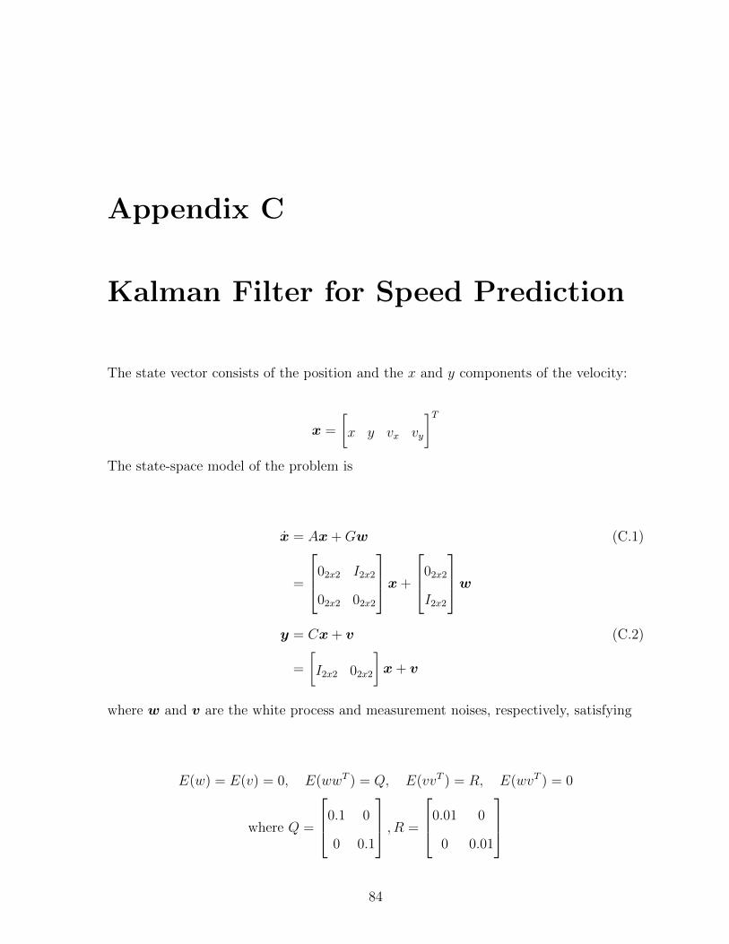
Appendix C
Kalman Filter for Speed Prediction
The state vector consists of the position and the x and y components of the velocity:
x =
[x y vx vy
]TThe state-space model of the problem is
x = Ax +Gw (C.1)
=
02x2 I2x2
02x2 02x2
x +
02x2
I2x2
w
y = Cx + v (C.2)
=
[I2x2 02x2
]x + v
where w and v are the white process and measurement noises, respectively, satisfying
E(w) = E(v) = 0, E(wwT ) = Q, E(vvT ) = R, E(wvT ) = 0
where Q =
0.1 0
0 0.1
, R =
0.01 0
0 0.01
84
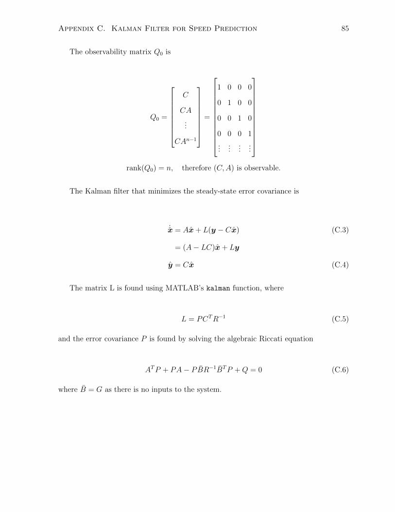
Appendix C. Kalman Filter for Speed Prediction 85
The observability matrix Q0 is
Q0 =
C
CA
...
CAn−1
=
1 0 0 0
0 1 0 0
0 0 1 0
0 0 0 1
......
......
rank(Q0) = n, therefore (C,A) is observable.
The Kalman filter that minimizes the steady-state error covariance is
˙x = Ax + L(y − Cx) (C.3)
= (A− LC)x + Ly
y = Cx (C.4)
The matrix L is found using MATLAB’s kalman function, where
L = PCTR−1 (C.5)
and the error covariance P is found by solving the algebraic Riccati equation
ATP + PA− PBR−1BTP +Q = 0 (C.6)
where B = G as there is no inputs to the system.

Bibliography
[1] R. Isaacs, Differential Games. New York: John Wiley and Sons, Inc., 1965.
[2] J. Lewin, Differential Games: Theory and Methods for Solving Game Problems with
Singular Surfaces. London: Springer-Verlag, 1994.
[3] J. Hespanha, M. Prandini, and S. Sastry, “Probabilistic pursuit-evasion games: A
one-step nash approach,” Proceedings of the 39th IEEE Conference on Decision and
Control, Sydney, Australia, vol. 3, pp. 2272–2277, 2000.
[4] J. Hespanha, H. Kim, and S. Sastry, “Multiple-agent probabilistic pursuit-evasion
games,” Proceedings of the 38th IEEE Conference on Decision and Control, Phoenix,
Arizona, vol. 3, pp. 2432–2437, 1999.
[5] R. Vidal, O. Shakernia, H. Kim, D. Shim, and S. Sastry, “Probabilistic pursuit-
evasion games: Theory, implementation, and experimental evaluation,” IEEE Trans-
actions on Robotics and Automation, vol. 18(5), pp. 662–669, 2002.
[6] S. LaValle, D. Lin, L. Guibas, J. Latombe, and R. Motwani, “Finding an unpre-
dictable target in a workspace with obstacles,” Proceedings of the IEEE International
Conference on Robotics and Automation, Albuquerque, New Mexico, pp. 737–742,
1997.
86
Bibliography 87
[7] A. AlDahak and A. Elnagar, “A practical pursuit-evasion algorithm: Detection and
tracking,” IEEE International Conference on Robotics and Automation, Roma, Italy,
pp. 343–348, 2007.
[8] B. Tovar and S. LaValle, “Visibility-based pursuit-evasion with bounded speed,” The
International Journal of Robotics Research, vol. 27(11-12), pp. 1350–1360, 2008.
[9] D. Li and J. Cruz, Jr., “A two-player stochastic pursuit-evasion differential game,”
Proceedings of the 46th IEEE Conference on Decision and Control, New Orleans,
LA, pp. 4057–4062, 2007.
[10] T. Shima and O. Golan, “Bounded differential games guidance law for dual-
controlled missiles,” IEEE Transactions on Control Systems Technology, vol. 14(4),
pp. 719–724, 2006.
[11] S. Bhattacharya, S. Hutchinson, and T. Basar, “Game-theoretic analysis of a visi-
bility based pursuit-evasion game in the presence of obstacles,” Proceedings of the
American Conference, St. Louis, Missouri, pp. 373–378, 2009.
[12] S. Bhattacharya and S. Hutchinson, “On the existence of nash equilibrium for a two-
player pursuit-evasion game with visibility constraints,” The International Journal
of Robotics Research, vol. 29(7), pp. 831–839, 2010.
[13] T. Muppirala, S. Hutchinson, and R. Murrieta-Cid, “Optimal motion strategies
based on critical events to maintain visibility of a moving target,” Proceedings of
the IEEE International Conference on Robotics and Automation, Barcelona, Spain,
pp. 3826–3831, 2005.
[14] J. Kim and M. Tahk, “Co-evolutionary computation for constrained min-max prob-
lems and its applications for pursuit-evasion games,” Proceedings of the Congress of
Evolutionary Computation, vol. 2, pp. 1205–1212, 2001.
Bibliography 88
[15] J. Ge, L. Tang, J. Reimann, and G. Vachtsevanos, “Hierarchical decomposition
approach for pursuit-evasion differential game with multiple players,” Proceedings of
the IEEE Aerospace Conference, 2006.
[16] D. Li, J. Cruz, Jr., G. Chen, C. Kwan, and M. Chang, “A hierarchical approach
to multi-player pursuit-evasion differential games,” Proceedings of the 44th IEEE
Conference on Decision and Control, Seville, Spain, pp. 5674–5679, 2005.
[17] A. Sun and H. Liu, “Multi-pursuer evasion,” AIAA Guidance, Navigation and Con-
trols Conference, Honolulu, HI, 2008.
[18] A. Bolonkin and R. Murphey, “Geometry-based parametric modeling for single-
pursuer/mutiple-evader problems,” Journal of Guidance, Control, and Dynamics,
vol. 28(1), pp. 145–149, 2005.
[19] S. Bopardikar, F. Bullo, and J. Hespanha, “On discrete-time pursuit-evasion games
with sensing limitations,” IEEE Transactions on Robotics, vol. 24(6), pp. 1429–1439,
2008.
[20] J. Durham, A. Franchi, and F. Bullo, “Distributed pursuit-evasion with limited-
visibility sensors via frontier-based exploration,” Proceedings of the IEEE Interna-
tional Conference on Robotics and Automation, pp. 3562–3568, 2010.
[21] B. Gerkey, S. Thrun, and G. Gordon, “Visibility-based pursuit-evasion with limited
field of view,” International Journal of Robotics Research, vol. 25(4), pp. 299–315,
2006.
[22] A. Antoniades, H. Kim, and S. Sastry, “Pursuit-evasion strategies for teams of mul-
tiple agents with incomplete information,” Proceedings of the 42nd IEEE Conference
on Decision and Control, Maui, HI, vol. 1, pp. 756–761, 2003.
Bibliography 89
[23] G. Wang and Z. Yu, “A pontryagins maximum principle for non-zero sum differen-
tial games of bsdes with applications,” IEEE Transactions on Automatic Control,
vol. 55(7), pp. 1742–1747, 2010.
[24] A. Starr and Y. Ho, “Nonzero-sum differential games,” Journal of Optimization
Theory and Applications, vol. 3(3), pp. 184–206, 1969.
[25] H. Sun, M. Li, and W. Zhang, “Infinite time nonzero-sum linear quadratic stochastic
differential games,” Proceedings of the 29th Chinese Control Conference, Beijing,
China, pp. 1081–1084, 2010.
[26] A. Akhmetzhanov, P. Bernhard, F. Grognard, and L. Mailleret, “Competition be-
tween foraging predators and hiding preys as a nonzero-sum differential game,”
Game Theory for Networks, pp. 357–365, 2009.
[27] A. Lim, X. Zhou, , and J. Moore, “Multiple objective risk-sensitive control and
stochastic differential games,” Proceedings of the 38th Conference on Decision &
Control, Phoenix, AZ, pp. 558–563, 1999.
[28] H. Choset, K. Lynch, S. Hutchinson, G. Kantor, W. Burgard, L. Kavraki, and
S. Thrun, Principles of Robot Motion: Theory, Algorithms, and Implementations.
Cambridge, MA: MIT Press, 2005.
[29] C. Goerzen, Z. Kong, and B. Mettler, “A survey of motion planning algorithms from
the perspective of autonomous uav guidance,” Journal of Intelligent and Robotic
Systems, vol. 57, pp. 65–100, 2010.
[30] Y. Hwang and N. Ahuja, “A potential field approach to path planning,” IEEE
Transactions of Robotics and Automation, vol. 8(1), pp. 23–32, 1992.
[31] S. LaValle, Planning Algorithms. Cambridge University Press, 2006.
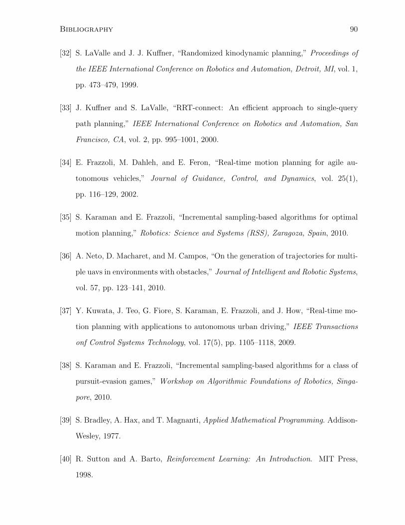
Bibliography 90
[32] S. LaValle and J. J. Kuffner, “Randomized kinodynamic planning,” Proceedings of
the IEEE International Conference on Robotics and Automation, Detroit, MI, vol. 1,
pp. 473–479, 1999.
[33] J. Kuffner and S. LaValle, “RRT-connect: An efficient approach to single-query
path planning,” IEEE International Conference on Robotics and Automation, San
Francisco, CA, vol. 2, pp. 995–1001, 2000.
[34] E. Frazzoli, M. Dahleh, and E. Feron, “Real-time motion planning for agile au-
tonomous vehicles,” Journal of Guidance, Control, and Dynamics, vol. 25(1),
pp. 116–129, 2002.
[35] S. Karaman and E. Frazzoli, “Incremental sampling-based algorithms for optimal
motion planning,” Robotics: Science and Systems (RSS), Zaragoza, Spain, 2010.
[36] A. Neto, D. Macharet, and M. Campos, “On the generation of trajectories for multi-
ple uavs in environments with obstacles,” Journal of Intelligent and Robotic Systems,
vol. 57, pp. 123–141, 2010.
[37] Y. Kuwata, J. Teo, G. Fiore, S. Karaman, E. Frazzoli, and J. How, “Real-time mo-
tion planning with applications to autonomous urban driving,” IEEE Transactions
onf Control Systems Technology, vol. 17(5), pp. 1105–1118, 2009.
[38] S. Karaman and E. Frazzoli, “Incremental sampling-based algorithms for a class of
pursuit-evasion games,” Workshop on Algorithmic Foundations of Robotics, Singa-
pore, 2010.
[39] S. Bradley, A. Hax, and T. Magnanti, Applied Mathematical Programming. Addison-
Wesley, 1977.
[40] R. Sutton and A. Barto, Reinforcement Learning: An Introduction. MIT Press,
1998.

Bibliography 91
[41] A. Rao, D. Benson, C. Darby, M. Patterson, C. Francolin, I. Sanders, and
G. Huntington, “Open-source general pseudospectral optimal control software.”
http://www.gpops.org, 2008.
[42] A. Rao, A Primer on Pseudospectral Methods for Solving Optimal Control Problems.
Gainesville, FL, January 2011.
[43] D. Kirk, Optimal Control Theory: An Introduction. Eaglewood Cliffs, NJ: Printice
Hall, 1970.
[44] G. Lau and H. Liu, “Online border patrol guidance algorithm for unmanned aerial
vehicles,” Proceedings of the AIAA Guidance, Navigation and Controls Conference,
Minneapolis, Minnesota, 2012.
[45] R. Siegwart and I. Nourbakhsh, Introduction to Autonomous Mobile Robots. MIT
Press, 2004.
[46] L. Dubins, “On curves of minimal length with a constraint on average curvature,
and with prescribed initial and terminal positions and tangents,” American Journal
of Mathematics, vol. 79, pp. 497–516, 1957.
[47] A. Shkel and V. Lumelsky, “Classification of the dubins set,” Robotics and Au-
tonomous Systems, vol. 34, pp. 179–202, 2001.


![Particle Swarm Optimization Algorithms for Autonomous ... · Bad Centers [1]. It has different deployment strategies implemented from where the moving algorithms start. The frontend](https://static.fdocuments.net/doc/165x107/5f0cf8567e708231d438082e/particle-swarm-optimization-algorithms-for-autonomous-bad-centers-1-it-has.jpg)