PATH INTEGRALS IN QUANTUM MECHANICS

BENJAMIN MCKAY

Abstract. These notes are intended to introduce the mathematically inclined

reader to the formulation of quantum mechanics via path integrals.

Contents

1. Introduction 12. The two slit experiment 23. How to find the amplitude of a path 44. The classical limit 85. Cutting and pasting 96. Example: the free particle 107. Example: the harmonic oscillator 138. The Schrodinger equation 179. Amplitudes as states 1810. Measurements and operators 1911. Insertions in the path integral 2112. Why the Hamiltonian operator represents energy 2313. Functional calculus and the operator equation of motion 2614. The functional Fourier transform 2715. Gaussian integrals 2816. Gaussian integrals with insertions 3117. Perturbation theory and Feynman diagrams 3218. Answers to the exercises 34References 39

“ I’m not making this up, youknow.”Anna Russell, The Ring of theNibelung

1. Introduction

This material is drawn largely from Feynman & Hibbs [2]. It is also helpfulto take a look the list of errata given by Styer [4]. I would like to thank themathematicians who sat through these lectures, and particularly Aaron Bertram,Jim Carlson, Javier Fernandez and Steve Gersten for helpful comments.

Date: November 19, 2001.

1

2 BENJAMIN MCKAY

Emitter of electrons Screen with two slits Detector

Figure 1. The two slit experiment

2. The two slit experiment

In the experiment shown in figure 2 we watch electrons strike a detector; eachone arrives like a drop of rain. Each electron is counted with a “click” and itsapproximate location recorded. The electrons coming in are counted up, and wefind the numbers of them (actually, the density) graphed in figure 2 on the nextpage. What is it?Guesses

(1) Each electron passes through either hole 1 or hole 2.(2) The number of electrons per second striking at a spot on the detector is the

sum of the number/second coming through hole 1 with the number/secondcoming through hole 2.

Lets check. Close hole 2, as in figure 2 on the facing page. The distribution ofelectrons is drawn in figure 2 on page 4. Now close hole 1. This is not working.Guess 2 is wrong! It would give us Imagine a breakwater in a harbour with twogaps for ships to pass through. What do the waves look like? Suppose we havetwo breakwaters: Ships go up and down like oscillating. The magnitude squared ofthis wave form looks a lot like the counting of electrons in the two slit experiment.Guess:Guesses

(3) For each point of the screen, there are complex numbers φ1 and φ2 (repre-senting contributions from each of the two holes) called amplitudes so thatthe probability of seeing an electron at that point of the screen is |φ1 + φ2|2with both holes open.

(4) If we close a hole, say hole 2, then φ2 is replaced by 0.This works. The humps in figures 2 on page 4 and 2 on page 5 show |φ1|2 and |φ2|2but adding φ1 + φ2 gives interference from phases.

Now lets try lots of holes as in figure 2 on page 7: Then we have to add upcomplex amplitudes for each hole at each point of the detector screen. Suppose wehave lots of screens too, as in figure 2 on page 8. Then we have to add up not just

3

0

0.2

0.4

0.6

0.8

1

–6 –4 –2 2 4 6

x

Figure 2. The density of electrons coming in at the detector

Emitter of electrons DetectorScreen with one slit shut

Figure 3. Closing one hole

a contribution from each hole, but from a choice of which hole to pass through ineach screen: a choice of route that the electron could pick in travelling from emitterto screen.

4 BENJAMIN MCKAY

0.2

0.4

0.6

0.8

1

–6 –4 –2 2 4 6

x

Figure 4. The density of electrons after we close the right hole

In the limit, we have a continuum of screens, but each of them is all holes. (Sothere aren’t actually any screens at all.) We find the sum over possible routesbecomes a path integral. So the probability of finding an electron at a point x1 ofthe screen is

Prob (x1) =∣∣∣∣∫ [dx]φ [x(t)]

∣∣∣∣2where the integral sums over all paths x(t) from the emitter to the point x1, andφ [x(t)] means the amplitude for this path.

3. How to find the amplitude of a path

A plane wave in empty space has linearly evolving phase. By analogy, in order toget wave-like behaviour of amplitudes, we expect to have evolution of phase alonga product of paths to be the sum of the phases for each. This suggests:

Guesses

(5)

φ

(· A // · B // ·

)= φ

(· A // ·

)φ

(· B // ·

)in other words: amplitudes for events in succession multiply.

5

0

0.2

0.4

0.6

0.8

1

–6 –4 –2 2 4 6

x

Figure 5. The density of electrons after we close the left hole

With this given, finding amplitudes is a local problem. In particular, for a pathwhich is just a single point

φ(·) = 1

by the multiplication of amplitudes. Let us find the amplitude of a little piece ofpath, say infinitesimally large. This is just a tangent vector to the path. So

φ ( // ) = 1 + correction .

To have pure linear evolution of phase in empty space, we want the correction tojust push the phase around, (i.e. to be tangent to the unit circle in the complexnumbers) so to be imaginary:

φ ( // ) = 1 + iL

for some quantity L which depends only on the tangent vector to our curve (so L is areal valued function on the tangent bundle). Multiplying together the contributionsalong a whole curve:

φ [x(t)] = ei∫

L(x(t),x(t)) dt.

To make rescaling easier, we will include a rescaling constant ~. This ~ must havethe same units as L. Why? Because to take an exponential

ez = 1 + z +z2

2+ . . .

6 BENJAMIN MCKAY

0

0.2

0.4

0.6

0.8

1

–6 –4 –2 2 4 6

x

Figure 6. The density of electrons expected to come in at the detectorShips tie up here

Dry land

First breakwall: one hole Second breakwall: two holes

Open sea

Figure 7. A harbour

7

–0.4

–0.2

0

0.2

0.4

0.6

0.8

1

–6 –4 –2 2 4 6

x

Figure 8. Waves lifting ships in a harbour

Emitter of electrons DetectorScreen with many slits

Figure 9. Lots of holes

we have to be able to add together all powers of z. But the units of z2 will onlyequal those of z if z is unitless. Therefore we put in an ~ just to balance off theunits.

8 BENJAMIN MCKAY

Emitter of electrons DetectorLots of screens with lots of slits

Figure 10. Lots of screens with lots of holes

Summing up (both literally and figuratively), the probability of seeing an electronat x1 is

Prob (x0) =∣∣∣[dx]e i

~∫

dt L(x(t),x(t))∣∣∣2

where the integral is over all paths from emitter to x1. What is L?Guesses

(6) L is the Lagrangian of the classical theory.Justifications

• It works!• The Lagrangian is the only function we know on the tangent bundle which

can determine the entire classical theory, i.e. the classical paths.Remark 1 The paths we sum over include those going back and forth many times,as in figure 3 on the facing page.Remark 2 Aaron’s lectures only allowed Lagrangians to depend on position and

velocity. Sometimes it is convenient to allow them to depend on time as well—butnot for studying fundamental physics where we want to assume that the laws ofphysics are independent of time. However, in a lab, the potential energy function(which is part of the Lagrangian) may change with time because objects in the labequipment might move over time. We keep track of this in the potential energy,in lieu of trying to keep track of all particles in the universe directly in our math-ematical model. How we go about “averaging” all of the ambient universe into apotential function is a serious question which we probably won’t return to. Butthese issues are already present in classical physics.

4. The classical limit

If L is a typical Lagrangian like

L =m

2

∣∣∣∣dxdt∣∣∣∣2 − V (x)

9

Emitter of electrons Detector

Figure 11. A path which doubles back several times before hit-ting the detector

then the action S =∫Ldt has units of mass length2/time, and therefore to obtain

unitless quantities S/~ in our exponential, ~ has the same units. If we fix a lengthscale to measure in based on the size of physical phenomena we want to study, thenhaving ~ small is the same as studying large objects (or very massive ones).

The numbers

S =∫dtL

will become huge, and vary enormously with slight changes in path, and the complexnumbers e

i~ S will oscillate wilding in phase (i.e. direction in the complex plane).

But near a classical path, the integral of the Lagrangian does not vary as much as itdoes at other places, so that these numbers e

i~ S all point in nearly the same direction

for paths close to a classical path. These add up to a large contribution, comparedto the wildly varying phases away from a classical path, which (we imagine) canceleach other out.

In the ~ → 0 (semiclassical) limit, only classical paths contribute, explainingtheir significance in large scale physics.

5. Cutting and pasting

The rule

φ

(· A // · B // ·

)= φ

(· A // ·

)φ

(· B // ·

)which obviously holds for

φ = ei~ S

allows us to cut the path integral in two. First, lets write

〈x1, t1|x0, t0〉 =∫

[dx]x1,t1x0,t0e

i~ S

where the integral is carried out over paths which leave the point x0 at time t0 andarrive at x1 at time t1. Then splitting paths in two at an intermediate time tm

10 BENJAMIN MCKAY

Emitter of electrons Detector

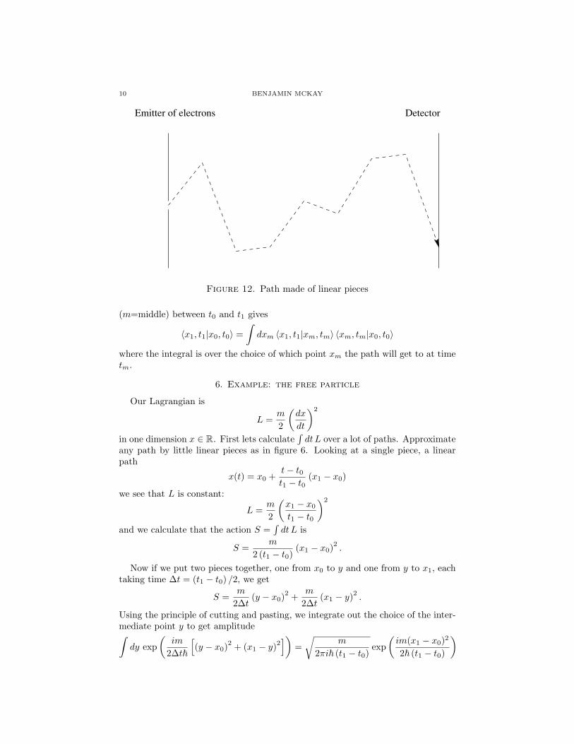
Figure 12. Path made of linear pieces

(m=middle) between t0 and t1 gives

〈x1, t1|x0, t0〉 =∫dxm 〈x1, t1|xm, tm〉 〈xm, tm|x0, t0〉

where the integral is over the choice of which point xm the path will get to at timetm.

6. Example: the free particle

Our Lagrangian is

L =m

2

(dx

dt

)2

in one dimension x ∈ R. First lets calculate∫dtL over a lot of paths. Approximate

any path by little linear pieces as in figure 6. Looking at a single piece, a linearpath

x(t) = x0 +t− t0t1 − t0

(x1 − x0)

we see that L is constant:

L =m

2

(x1 − x0

t1 − t0

)2

and we calculate that the action S =∫dtL is

S =m

2 (t1 − t0)(x1 − x0)

2.

Now if we put two pieces together, one from x0 to y and one from y to x1, eachtaking time ∆t = (t1 − t0) /2, we get

S =m

2∆t(y − x0)

2 +m

2∆t(x1 − y)2 .

Using the principle of cutting and pasting, we integrate out the choice of the inter-mediate point y to get amplitude∫dy exp

(im

2∆t~

[(y − x0)

2 + (x1 − y)2])

=√

m

2πi~ (t1 − t0)exp

(im(x1 − x0)2

2~ (t1 − t0)

)

11

the amplitude from going along two linear pieces, with an arbitrary choice of mid-point.1 To handle 3 pieces, we carry out two integrations over midpoints in thesame manner and find exactly the same answer.

Continuing in this manner, if we divide up an interval of time from t0 to t1 intopieces of duration ∆t = (t1 − t0)/N for a large N , we get amplitude√

m

2πi~ (t1 − t0)exp

(im(x1 − x0)2

2~ (t1 − t0)

)for traveling along a piecewise linear path with breakpoints at times t0, t0+∆t/N, . . . , t1.Since this expression is independent of how many break points we use, in the limitas N →∞ we obtain, for any points x0, t0 and x1, t1:

〈x1, t1|x0, t0〉 =√

m

2πi~ (t1 − t0)exp

(im(x1 − x0)2

2~ (t1 − t0)

).

Therefore the probability of the particle arriving at x1 at time t1, if it was at x0

at time t0, is

Prob (x1) =∣∣∣∣√ m

2πi~ (t1 − t0)exp

(im(x1 − x0)2

2~ (t1 − t0)

)∣∣∣∣2 =m

2π (t1 − t0) ~

which is independent of x1 so it is equally likely to be anywhere. The probabilitythat the particle is somewhere at all is∫

Prob (x1) dx1 = ∞.

So it isn’t really a probability at all.Exercise 1. Wave functions

Given a function φ0(x) define

(1) φ(x, t) =∫〈x, t|x0, 0〉φ0 (x0) dx0

where the expression〈x, t|x0, 0〉

is the free particle amplitude computed above. Show that(a) The function φ(x, t) satisfies the Schrodinger equation for the

free particle∂φ

∂t=

i~2m

∂2φ

∂x2.

(b)

φ(x, t) → φ0 (x) in L2 as t→ 0.

(c) ∫|φ(x, t)|2 dx

is independent of t (unitary evolution).

1The evaluation of Gaussian integrals will be discussed in section 15 on page 28.

12 BENJAMIN MCKAY

To handle the infinity of the “probability”∫

Prob dx1, we must “smear” the parti-cles, giving them their own amplitude functions, say φ(x, t), so that the probabilitythat the electron is between x0 and x0 + ∆x is∫ x0+∆x

x0

|φ (x, t0)|2 dx

and allow these amplitude functions to evolve via equation 1 on the page before.Call the function φ the wave function or state of the electron.To handle the free particle in n dimensional space Rn, treat it as a sum of

independent contributions to the Lagrangian, which get exponentiated:

〈x1, t1|x0, t0〉 =(

m

2πi~ (t1 − t0)

)n/2

exp

(im ‖x1 − x0‖2

2~ (t1 − t0)

).

Exercise 2. The free particle on the circle(a) Take a particle α(t) on a circle R/2πRZ, with R > 0, and the

same free particle Lagrangian

L =m

2

(dα

dt

)2

.

Calculate〈α1, t1|α0, t0〉

for−πR ≤ α0, α1 < πR.

Hint: you will have to sum over all “winding numbers” of apath around the circle.

(b) Express your answer in terms of the ϑ function

ϑ(z, τ) =∑N∈Z

exp(πiN2τ + 2πiNz

).

(c) Use the functional identity

ϑ(z, τ) = exp(πi

4

)τ−1/2 exp

(−πiz2

τ

)ϑ

(z

τ,−1

τ

)to find that

〈α1, t1|α0, t0〉 =1

2πRϑ

(α1 − α0

2πR,−~ (t1 − t0)

2πR2m

).

(d) Now show directly from the definition of ϑ that this ampli-tude 〈α1, t1|α0, t0〉 satisfies the same properties that you foundfor the free particle amplitude in the previous problem: itis a Green’s function for the same free particle Schrodingerequation, and as a Green’s function, it propagates a functionφ(α, t) preserving∫

R/2πRZdα |φ(α, t)|2

over all time t. (Hint: see pages 4 and 5 of Mumford [3].)Note that ϑ(z, τ) is defined by an “oscillatory sum” for realvalues of τ (real τ is the boundary of the Siegel half-plane),

13

but still makes sense in this context as a pseudodifferentialoperator.

Exercise 3. Fourier series

Use Fourier transforms [or Fourier series] in the x [or α] variableto solve the free particle Schrodinger equation on the line [or thecircle], expressing the answer as

φ(x, t) =∫G (x, t, x0, t0)φ0 (x0) dx0

so that φ satisfies the free Schrodinger equation, and φ = φ0 att = t0. Compare to the amplitude coming from the path integral.

Exercise 4. Twisted sectors

Consider an s-fold covering of a circle:

α ∈ R/2πRZ 7→ β = sα ∈ R/2πRZ.

Split each function φ(α) on the covering circle into Fourier series,

φ (α) =∑k∈Z

ckeikα

and write it as

φ (α) =s−1∑r=0

φr (α)

whereφr (α) =

∑q∈Z

cqs+rei(qs+r)α.

Interpret this as defining line bundles on the base circle. Showthat φ(α) evolves as a free particle wave function precisely if eachof the functions φr (α) evolves as in equation 1 on page 11 withthe amplitudes

〈β1, t1|β0, t0〉r =1

2πRϑ[r/s

0

] (z, τ)

where

z =β1 − β0

2πRand τ = − ~ (t1 − t0)

2πm(R/s)2

and the expression ϑ[r/s0

] means the ϑ-function with characteris-

tics, defined by

ϑ[ab

](z, τ) =∑N∈Z

exp(πi(a+N)2τ + 2πi(a+N)(z + b)

).

7. Example: the harmonic oscillator

The Lagrangian is

L =m

2

((dx

dt

)2

− ω2x2

).

14 BENJAMIN MCKAY

xcl(t)

xcl(t) + y(t)

Figure 13. Perturbing a classical path

We will find the amplitude 〈x1, t1|x0, t0〉 . It suffices to find 〈x1, T |x0, 0〉, becausethe Lagrangian does not depend (directly) on time. Note that the Lagrangian isquadratic. So

S[x] =∫dtL (x(t), x(t))

is quadratic in x.If we take a path x(t) we can split it into a classical path xcl(t) (satisfying the

Euler–Lagrange equations) and a “perturbation” y(t) with y(0) = y(T ) = 0, as infigure 7.

Since S[x] is quadratic, we can write it as S[x, x] a bilinear form, and find

S[x] = S [xcl + y]

= S [xcl] + 2S [xcl, y] + S [y]

Exercise 5.

Write S [xcl, y] as an integral.

The Euler–Lagrange equations say perturbing a classical path has no influenceon the action, to first order, so

S [xcl, y] = 0.

Therefore

S[x] = S [xcl] + S [y]

15

and the amplitude is

〈x1, T |x0, 0〉 =∫

[dx]eiS[x]/~

=∫

[dy]eiS[xcl+y]/~

=∫

[dy]eiS[xcl]/hbareiS[y]/~

= eiS[xcl]/~∫

[dy]eiS[y]/~.

The [dy] integral is an integral over all perturbations of the classical path xcl(t), sothese y(t) must vanish at times t = 0 and t = T . Hence we have factored

〈x1, T |x0, 0〉 = eiS[xcl]/~︸ ︷︷ ︸Depends on x0,x1,T

〈0, T |0, 0〉︸ ︷︷ ︸Depends on T

into a purely classical contribution, and a path integral.Exercise 6. The action on classical paths

(a) Find the Euler–Lagrange equations of the harmonic oscillator.(b) Find the classical path xcl(t) passing through x0 at time t = 0

and x1 at time t = T . Assume that ωT is not an integer.(c) Calculate the action S [xcl] along this classical path. You

should get

S [xcl] =∫dtL (x(t), x(t))

=mω

2 sin (ωT )(cos (ωT )

(x2

0 + x21

)− 2x0x1

).

Now we expand the perturbation into eigenfunctions of the Sturm–Liouville op-erator. What is that?Exercise 7. Sturm–Liouville operators

Recall that the Euler–Lagrange equations for a path xcl(t) witht0 ≤ t ≤ t1 are S′ [xcl] = 0, where

S′[x]y =∫dt

(∂L

∂x− d

dt

∂L

∂x

)y.

(a) Show that if S′ [xcl] = 0, then for any functions y(t), z(t)vanishing at t = t0 and t = t1:

S′′ [xcl] (y, z) =∫ (

∂2L

∂x2z(t) +

∂2L

∂x∂xz(t)− d

dt

(∂2L

∂x∂xz(t) +

∂2L

∂x2z(t)

))y(t).

In particular if we ask that S′′ [xcl] (y, z) = 0 for all y then weobtain a second ordinary differential operator in z which wewrite S′′[x](z), called the Sturm–Liouville operator.

(b) Why is the Sturm–Liouville operator self-adjoint?(c) Show that the Sturm–Liouville operator of the harmonic os-

cillator is

S′′[x] = −m d2

dt2−mω2.

16 BENJAMIN MCKAY

Show that the functions

yk(t) =

√2T

sin(πkt

T

)are an orthonormal basis of its eigenfunctions, with eigenval-ues

λk = m

((πk

T

)2

− ω2

).

So in the basis yk(t) the quadratic function S is now given by a diagonal matrix:

S =

λ1

λ2

λ3

. . .

and the path integral is a Gaussian integral:∫

[dy]eiS[y]/~ =1√

det(

S′′

2π

)(essentially; see section 15 on page 28 for more). How do we calculate the determi-nant? It is the product of eigenvalues:

1√det(

S′′

2π

) =1√∏k

λk

2π

=1√∏

km2π

((πkT

)2 − ω2)

=1√√√√√√

∏k

mπk2

2T 2

∏k

(1− ω2T 2

k2π2

)︸ ︷︷ ︸Ahlfors [1] pg. 197

=1

F (T )√

sin(ωT )ωT

This F (T ) is annoying: it has to be

F (T ) =

√∏k

mπk2

2T 2

which is divergent. But if we ignore it, we have

〈x1, T |x0, 0〉 =eiS[xcl]/~

F (T )√

sin(ωT )ωT

.

Exercise 8. Normalizing the amplitude

17

Taking ω → 0 we should get the same result as the free particle.Note that F (T ) above is independent of ω. Use this to find F (T )and to show that the final amplitude is

(2)

〈x1, T |x0, 0〉 =√

m

2πi~T

(ωT

sin (ωT )

)1/2

exp

(im

2~T

((x2

0 + x21

)ωT

tan (ωT )− 2x0x1ωT

sin (ωT )

)).

Exercise 9. The Schrodinger pictureGet Maple (or a long hand calculation) to show that this functionis a Green’s function for the Schrodinger equation for the harmonicoscillator, which is

i~∂φ

∂t= − ~2

2m∂2φ

∂x2+mω2x2φ.

8. The Schrodinger equation

We have insisted (but by no means proven) that our amplitudes

〈x1, t1|x0, t0〉

must provide a transformation of wave functions preserving probabilities, i.e. if

(3) φ1 (x1) =∫dx0 〈x1, t1|x0, t0〉φ0 (x0)

then we require ∫dx1 |φ1 (x1)|2 =

∫dx0 |φ0 (x0)|2 .

This is essential to ensure that if we start with |φ0|2 a probability density (i.e.nonnegative of unit integral), then we end up with another probability density.

Therefore equation 3 is an equation of unitary evolution. Write it as

U (t0, t1)φ0 = φ1.

This U (t0, t1) is a unitary operator on complex valued functions. Therefore itsinverse is its adjoint:

U (t1, t0) = U (t0, t1)−1 = U (t0, t1)

∗.

In terms of integrals, this is just

(4)∫dx0 〈x1, t1|x0, t0〉 〈x′1, t1|x0, t0〉

∗ = δ (x0 − x′0)

(where the ∗ here means complex conjugate of a complex number).Differentiating and then setting t1 = t0, and defining

H (t0) = i~∂

∂t1U (t0, t1)

∣∣∣∣t1=t0

we find that this H (t0) is a self-adjoint operator.2 Call it the Hamiltonian operator.Another way to say this: the Lie algebra of the unitary group consists of the skew-adjoint operators. But every skew-adjoint operator is just A = −iH where H is

2For the present, we will write hats on operators to indicate that they are self-adjoint operators.

18 BENJAMIN MCKAY

self-adjoint. We put in the ~ for convenience. Then we recover the unitary evolutionfrom

(5)∂φ

∂t= − i

~H(t)φ

which is the Schrodinger equation.3

9. Amplitudes as states

Now suppose that we carry out an experiment, in which a particle hits a certainspot if the particle has a certain property, and doesn’t hit it otherwise. (In somemanner, perhaps involving many particles, all experiments have this form.) The wayin which we arrange the experimental apparatus, our lab equipment, is describedby a Lagrangian, say Lexperiment. Therefore the probability that the particle hasthe property is

Prob =∣∣∣∣∫

spot

dx1 〈x1, t1|x0, t0〉experiment φ (x0)∣∣∣∣2

where φ is the wave function of the particle at the time t0 when the experimentstarted.

If the particle’s wave function was a δ function at a point x0, this would give∣∣∣〈x1, t1|x0, t0〉experiment

∣∣∣2 .So the amplitude

〈x1, t1|x0, t0〉as a function of x1 is the wave function at time t1, so that the original wave functionat time t0 was a δ function.

On the other hand, if we want to be certain about the precise outcome of theexperiment, then we want a δ function to come out, say at a point xtarget.∫

dx1 〈x1, t1|x0, t0〉experiment φ (x0) = δ (x1 − xtarget) .

What function φ should we use? From equation 4 on the preceding page, we seethat we can take

φ (x0) = 〈xtarget, t1|x0, t0〉∗experiment .

By invertibility of unitary evolution, this function is the only function we can use.Therefore the complex conjugate 〈x1, t1|x0, t0〉∗experiment of the amplitude is the statea particle must be in at time t0 to have complete certainty that it will end up atx1 at time t1.

Writeψ (x0) = 〈x1, t1|x0, t0〉∗experiment .

This is the state that a particle must be in at time t0 to have certainty of its beingat x1 at time t1. So each experimental outcome has associated with it a state ψ,

ψ(x) = 〈x, t1|x0, t0〉 .

3For an arbitrary Lie group, instead of just a unitary group, we would prefer to call a Lie

equation.

19

In this case, we will say that it is the state of being at x1 at time t1. The amplitudeof a particle in state φ (x0) ending up at x1 at time t1 is∫

dx0 ψ∗ (x0)φ (x0)

which we write as an inner product

〈ψ, φ〉 .

In general, the probability of a particle represented by φ at time t0 behaving acertain way at a given time t1 is given by

|〈ψ, φ〉|2

where ψ is the state associated to that behaviour.

10. Measurements and operators

The expected value of an experimental measurement (which we assume to be areal number) is the sum over all possible outcomes a of

aProb(a).

Let us call A the quantity we are trying to measure. Then let ψa be the staterepresenting A = a. The expected value of A for a particle in state φ is∫

da a |〈ψa, φ〉|2 =∫da a

(∫dxψa(x)φ∗(x)

)(∫dx′ ψ∗a (x′)φ (x′)

)=∫dx dx′ φ∗(x) 〈x|A|x′〉φ (x′)

where we have written

〈x|A|x′〉 =∫da aψa(x)ψ∗a (x′) .

Exercise 10.

Show that〈x|A|x′〉∗ = 〈x′|A|x〉 .

Use this to show that the operator

Aφ(x) =∫dx′ 〈x|A|x′〉φ (x′)

is self-adjoint in the L2 norm.Exercise 11.

(a) Show that the expected value of A in state ψa(x) is a.(b) Show that

Aψa(x) = aψa(x).

These ψa(x) are the eigenfunctions of the operator A, and these a values are theeigenvalues.Exercise 12. Measuring position

Suppose that A is the measurement of position at time t0.

20 BENJAMIN MCKAY

(a) Show thatψx0(x) = δ (x− x0)

and thatAφ(x) = xφ(x).

Consequently, we will write this operator as x.(b) Find the function 〈x′|x|x〉.

Exercise 13. Measuring momentum(a) Let us first return to classical mechanics. Recall from Aaron’s

lectures4 that the Hamiltonian vector field ~H associated to afunction H(x, p) (on the cotangent bundle) is

~H =∂H

∂p

∂

∂x− ∂H

∂x

∂

∂p.

Also, the observables of classical mechanics are functions onthe cotangent bundle. So observables F (x, p) have “dynam-ics” associated to them: the flow of the vector field ~F . Showthat the flow of the vector field ~p (i.e. taking Hamiltonianfunction H(x, p) = p) is translation in the x variables, leavingp fixed.

(b) Suppose that we write p for the operator

pφ(x) = −i~∂φ∂x.

Show that this operator is self-adjoint.(c) Taking p as Hamiltonian operator, H = p, plug it into the

Schrodinger equation 5 on page 18 and integrate it to showthat the associated evolution is given by

U (t0, t1)φ (x1) = φ (x1 − (t1 − t0)) .

This should explain why this operator is called momentumand written p: the associated evolution is through translationsin the q variables.

(d) Find the eigenfunctions and eigenvalues of p.(e) Find the function

〈x′|p|x〉 .Exercise 14.

Calculate[x, p] = xp− px

Exercise 15. Momentum representation(For now) write the Fourier transform as

φ(p) =∫dx e−ixp/~φ(x)

(a) Show that the operator p becomes the operator

pφ(p) = pφ(p).

(b) What happens to the position operator x?

4The gentle reader will pardon me for not maintaining his distinction between q and x.

21

(c) What is the inverse of this Fourier transform? (Get the con-stants right.)

(d) What constant c do we have to take so that∫c dp

∣∣∣φ(p)∣∣∣2 =

∫dx |φ(x)|2?

11. Insertions in the path integral

The operator x which gives the expected position of a particle applies only towave functions at a given time t0 like

expected position at time t0 =∫dxφ (x, t0)

∗xφ (x, t0) .

If we only know the wave function at earlier and later times, say at times t0 andt1, and we want its expected position at an intermediate time tm then this is givenby taking the amplitude to get to a point xm, multiplying by xm, and taking theamplitude to get from xm:∫

dx1 dx0 dxm φ (x1, t1)∗ 〈x1, t1|xm, tm〉xm 〈xm, tm|x0, t0〉φ (x0, t0)

which we will write as∫dx1 dx0 φ (x1, t1)

∗ 〈x1, t1|x (tm) |x0, t0〉φ (x0, t0) .

By cutting and pasting,

〈x1, t1|x (tm) |x0, t0〉 =∫

[dx(t)]ei~ S x (tm)︸ ︷︷ ︸

A number!

so that expected position at an intermediate time tm is expressed in terms of a pathintegral with x (tm) inserted into it. Similarly, we can calculate any operator F (x)at time tm by inserting F (x (tm)) into the path integral.Exercise 16. Momentum in the path integral

Show that expected momentum at time tm is calculated from thewave function in the same manner as above for position, using∫

dp φ (x1, t1)∗ 〈x1, t1|p (tm) |x0, t0〉φ (x0, t0)

but where the “matrix elements”

〈x1, t1|p (tm) |x0, t0〉are calculated by taking the amplitudes

〈x1, t1|x+ y, tm〉 peipy/~ 〈x, tm|x0, t0〉and integrating out the intermediate position x and “jump” y, andthe momentum value p. So the interpretation is that the particlemoves along from x0 to x, and then jumps to x+y (see figure 11 onthe following page) with a contribution eipy/~ (which is the ampli-tude for a free particle to move from x to x+y with momentum p),and then the particle moves from x to x1. We measure the momen-tum during the jump to be p. But the “jump” is instantaneous.

22 BENJAMIN MCKAY

Emitter of electrons Detector

Figure 14. Measuring momentum with path integrals; we usepaths with jumps

Taking any functions A(x) and B(x) we can plug them into the path at twodifferent times ∫

[dx]ei~ S[x]A (x (ta))B (x (tb))

to calculate A (x (ta))B (x (tb)) . But this doesn’t quite work: if we expand outthe result in terms of amplitudes up to different times, we find that this computesA (x (ta))B (x (tb)) if ta > tb but computes B (x (tb))A (x (ta)) if ta < tb. Thereforewe define the time ordered product

T [A (x (ta))B (x (tb))] = θ (ta − tb)A (x (ta))B (x (tb))+θ (tb − ta)B (x (tb))A (x (ta))

where

θ(t) =

1 if t > 012 if t = 00 if t < 0

.

Exercise 17. Calculating HamiltoniansWe still haven’t indicated how to write down the Hamiltonian op-erator of any quantum systems, except the free particle and theharmonic oscillator. Suppose that you have a Lagrangian L0 andyou know its Hamiltonian operator H0(t). Make a new Lagrangianby

L (x, x) = L0 (x, x)− V (x)for some function V (x). Lets try to find the associated HamiltonianH(t).(a) First, we need to express H0 in terms of a path integral. Show

that

(6) H0 (t)φ(x) = i~d

dε

∣∣∣∣ε=0

∫〈x, t+ ε|y, t〉0 φ(y) dy.

where the amplitude with a zero subscript

〈x, t+ ε|y, t〉0

23

means that it is computed with a path integral containing L0

instead of L.(b) Next, we need to write amplitudes for L in terms of those for

L0. Writing

exp(i

~S[x]

)= exp

(i

~S0[x]

)exp

(− i

~

∫dt V (x (t))

),

expand out the second exponential factor, and derive theequation

〈x, t+ ε|y, t〉 =∞∑

k=0

1k!

(−i~

)k ∫ t+ε

t

dt1 . . .

∫ t+ε

t

dtk 〈x, t+ ε|T [V (x (t1)) . . . V (x (tk))] |y, t〉0 .

(c) Differentiate this expression with

d

dε

∣∣∣∣ε=0

to findH(t) = H0(t) + V (x) .

(d) IfL =

m

2x2 − V (x)

show that

H(t) = − ~2

2m∂2

∂x2+ V (x).

(e) Show that this is what you get from taking the Legendre trans-form (see Aaron’s notes) of of the Lagrangian and then replac-ing p variables by p operators and x variables by x operators.

12. Why the Hamiltonian operator represents energy

We want to see that the operator H has some relation to the Hamiltonian func-tion H, at least in the semiclassical limit.Exercise 18. The Hamilton–Jacobi equation

(It would have been better to see this in Aaron’s lectures.) Con-sider the picture of classical paths as trajectories of a flow

~H =∂H

∂p

∂

∂x− ∂H

∂x

∂

∂p.

The phase space maps to the configuration space by (x, p) 7→ x.Fix a particular point of configuration space x0, and look at thefiber of this map above that point. In figures 12 on the next pageand 12 on page 25 this fiber is a vertical line.(a) Fix times t1 > t0. Consider the map p0 7→ x1 defined by

taking an initial momentum p0 (a point of the fiber) and thenfollowing along the flow from (x0, p0) for time t1 − t0 to apoint (x1, p1). Looking at the expression of the Hamiltonianvector field above, under what conditions will it be true thatfor sufficiently small times t1 − t0 the map p0 7→ x1 is a localdiffeomorphism near some fixed value of p0? (Essentially theidea is that in the phase diagram, the x components of the

24 BENJAMIN MCKAY

–2

–1

0

1

2

p

–2 –1 1 2

x

Figure 15. The phase flow of a classical pendulum, indicating thelevels of the Hamiltonian

vector ~H are all different at different points of the fiber, atleast locally.) For what positions and times does this work forthe harmonic oscillator?

(b) Suppose that this map p0 7→ x1 is a diffeomorphism. Nowconsider the action S = S (x1, t1) obtained by integrating theLagrangian along the classical path that leaves x0 at time t0and reaches x1 at time t1. Consider the extended phase spacewith coordinates (x, p, t), and the 1-form ξ = p dx −H dt onthat space. The flow on the extended phase space is given bythe vector field

~H =∂H

∂p

∂

∂x− ∂H

∂x

∂

∂p+∂

∂t.

Show that ~H dξ = 0. Now taking two points x1 and x1+∆x1

and two times t1 and t1 +∆t1, consider for each 0 ≤ s ≤ 1 theclassical path that leaves x0 at time t0 and arrives at x1+s∆x1

at time t1 + s∆t1. These paths form a rectangle in extendedphase space. By using Stoke’s theorem applied to ξ on thisrectangle, show that

∆S = S (x1 + ∆x1, t1 + ∆t1)− S (x1, t1)

25

–2

–1

0

1

2

p

–2 –1 1 2

x

Figure 16. The phase flow of a classical pendulum, indicatingphase velocity

is given by

∆S = p1 ∆x1 −H ∆t1 +O((∆x1)

2, (∆t1)

2).

(c) Show thatdS = p dx−H dt.

(d) Use this to see that the function S = S (x1, t1) satisfies theHamilton–Jacobi equation

∂S

∂t+H

(x,∂S

∂x, t

)= 0.

This says that if you allow yourself more time ∆t to get there,the classical path requires less action by about −H∆t, whereH is total energy at the end of that original path.

Exercise 19.

In the semiclassical limit, i.e. for ~ very small, we have seen thatonly classical paths contribute. Lets assume this.(a) For any two points x0, x1 and times t0 < t1, show that in the

semiclassical limit,

〈x1, t1|x0, t0〉 =∑

x

exp(i

~S[x]

)

26 BENJAMIN MCKAY

and that⟨x1, t1|H (tm) |x0, t0

⟩=∑

x

H (x (tm) , p (tm)) exp(i

~S[x]

)where the sum is over all classical paths x(t) which satisfy

x (t0) = x0 x (t1) = x1

and the momentum p(t) is the momentum along that classicalpath. (Hint: equation 6 on page 22.) So it looks like aninsertion of the classical Hamiltonian into the path integral.

It is in this sense that we say that the eigenvalues of H represent energy levels.

13. Functional calculus and the operator equation of motion

The action S[x] is a functional: it eats paths and gives numbers. We differentiateit like:

dS[x]y =d

dεS[x+ εy]

∣∣∣∣ε=0

where y is a perturbation of the path x.Writing

S[x] =∫ t1

t0

dtL (x(t), x(t))

we find

dS[x]y =∂L

∂xy

∣∣∣∣t=t1

t=t0

+∫ t1

t0

dt

(∂L

∂x− d

dt

∂L

∂x

)y(t).

We will also consider more general functionals, say F [x].If we take y to be a δ function:

y(t) = δ (t− tm)

then we will writeδF

δx (tm)= dF [x]y.

For example, if t0 < tm < t1, then

δS

δx (tm)=(∂L

∂x− d

dt

∂L

∂x

)∣∣∣∣t=tm

.

It is this which vanishes on classical paths.If y(t) vanishes at t = t0 and t = t1, then since we add all paths into the path

integral, ∫[dx]F [x] =

∫[d(x+ y)]F [x+ y] =

∫[dx]F [x+ y].

Therefore ∫[dx]dF [x]y = lim

ε→0

∫[dx]F [x+ εy]−

∫[dx]F [x]

ε

= 0.

(Stoke’s theorem). Allowing y to become a δ function,∫[dx]

δF

δx (tm)= 0.

27

In particular if F [x] = exp(iS[x]/~),

0 =∫

[dx]δF

δx (tm)

=∫

[dx]eiS/~ δS

δx (tm)

=

⟨x1, t1|

δS

δx (tm)|x0, t0

⟩shows that

δS

δx (tm)= 0.

This is Ehrenfest’s theorem or the operator equation of motion. For example, itsays that the expected acceleration of a free particle is zero. In general it says thata particle is expected to satisfy the Euler–Lagrange equations.Exercise 20.

Using integration by parts in the path integral, show that

T

[δS

δx (tA)x (tB)

]= i~ δ (tB − tA)

as operators.

14. The functional Fourier transform

To package all of the insertions into one object, consider a function J(t) vanishingat times t0 and t1 and let LJ be the new Lagrangian

LJ = L− J(t)x(t).

Exercise 21.

Starting with Lagrangian

L =m

2

(dx

dt

)2

− V (x)

show that this corresponds physically to adding an external forceJ(t).

Define the partition function

Z(J) =∫

[dx] exp(i

~SJ [x]

).

We can expand this out into

Z(J) =∫

[dx] exp(i

~S[x]

)exp

(− i

~

∫dt J(t)x(t)

)=∫

[dx] exp(i

~S[x]

) ∞∑k=0

1k!

(−i~

∫dt J(t)x(t)

)k

.

28 BENJAMIN MCKAY

Now take functional derivatives:

δ

δJ (t1). . .

δ

δJ (tk)

∣∣∣∣J=0

Z(J) =(−i~

)k ∫[dx] exp

(i

~S[x]

)x (t1) . . . x (tk)

=(−i~

)〈x1, t1|T [x (t1) . . . x (tk)] |x0, t0〉 .

This gives all possible insertions, contained in the functional Z(J). By definition,Z(J) is the Fourier transform of exp (iS[x]/~). It might be useful to write it as〈x1, t1|x0, t0〉J to emphasize the dependence on the initial and final points.

Physicists say that the insertions determine the partition function Z(J) by Taylorexpansion:

Z(J) = −i~∑ 1

k!〈x1, t1|T [x (t1) . . . x (tk)] |x0, t0〉 J (t1) . . . J (tk) .

I don’t know what this means, except that they clearly believe that the values ofall insertions determine the partition function, although I don’t see how.Exercise 22. The free particle partition function

Calculate Z(J) for the free particle. It helps to have some notationlike

J1(t) =∫ t

t0

J(u) du.

15. Gaussian integrals

We have used some Gaussian integrals already. Define

I(A, b) =∫

Rn

dx e−12 〈Ax,x〉+〈b,x〉

where A is a positive definite symmetric matrix. To calculate it:(1) Change variables to y = x−A−1b (so that y = 0 is the minimum point) to

get

I(A, b) = e12 〈A−1b,b〉I(A, 0).

(2) Diagonalize A by a rotation of the y variables

I(A, 0) = I(Λ, 0)

where

Λ =

λ1

λ2

. . .λn

is the matrix of eigenvalues of A.

(3) Use the identity

e−12 〈Λx,x〉 = e−λ1x2

1/2 . . . e−λnx2n/2

to getI(Λ, 0) = I (λ1, 0) . . . I (λn, 0) .

Now we are reduced to 1-dimensional integrals.

29

(4) Change variables yj =√λjxj to get

I (λj , 0) =1√λj

I(1, 0).

(5) Finally, the Liouville trick: use polar coordinates in the plane

I(1, 0)2 =∫

R2dx dy e−(x2+y2)/2

=∫ ∞

0

r dr

∫ π

−π

dθe−r2/2

= 2π∫ ∞

0

drd

dr

(−e−r2/2

)= 2π

ThereforeI(1, 0) =

√2π.

Putting it together

I(A, b) =e

12 〈A−1b,b〉√det(

A2π

) .The final answer does not involve the dimension n. By analytic continuation, thesame equation holds for any complex matrix A with positive definite real part, andany complex vector b.

For Q a real definite symmetric matrix (maybe not positive definite) we willdefine the oscillatory integral

J(Q, b) =∫

Rn

ei2 〈Qx,x〉+〈b,x〉

(which a priori is not integrable) as a limit

J(Q, b) = limP→0

I(P − iQ, ib) =e−

i2 〈Q−1b,b〉√

det(−iQ2π

)where the limit is taken as the positive definite matrix P goes to zero. The trickypart is pulling out the −i in the determinant. Diagonalize Q, say

Q =

−λ1

−λ2

. . .−λn

µ1

µ2

. . .µp

with all λj , µk > 0. The square root that we use on P − iQ has branch set up sothat it gives positive real numbers on positive real numbers. So on iλj it gives√

iλj = eπi/4√λj ,

30 BENJAMIN MCKAY

and on −iµk it gives √−iµk = e−πi/4√µk.

So we get √det(−iQ2π

)= e−πi Index(Q)/4

√det(Q

2π

).

Note that this index is the index of inertia (also known as the signature), not theFredholm index. Finally:∫

Rn

ei2 〈Qx,x〉+〈b,x〉 = eπi Index(Q)/4 e

i2 〈Q−1b,b〉√det(

Q2π

)Exercise 23. Large radius limit

Use Gaussian integrals to show that the amplitude

〈α1, t1|α0, t0〉of a free particle on the circle of radius R approaches the amplitudeof a free particle on the line as the radius R goes to infinity. Hint:the ϑ function looks like a Riemann sum.

Exercise 24. Constant force fieldsFor a particle in a constant external field f , with Lagrangian

L =m

2x2 + fx

show that the amplitude for travelling between two points is

〈x1, t1|x0, t0〉 =( m

2πi~T

)exp

(i

~

[m (x1 − x0)

2

2T+

12fT (x0 + x1)−

f2T 3

24m

])where T = t1 − t0. The Hamiltonian is

H =p2

2m− fx.

Express the eigenfunctions of H in terms of the Airy function.Draw the eigenfunction with lowest eigenvalue and interpret thepicture.

Exercise 25.Using Fourier transforms of distributions (i.e. generalized func-tions) show that we can “define” the oscillatory integral∫

Rn

ei2 〈Qx,x〉 dx =

∫f(x) dx

as the limitlimp→0

f(p)

of its Fourier transform, and that we obtain the expected answer.Exercise 26.

Using a Gaussian integral, being careful about phase, show thatthe phase in our calculation of the amplitude 〈x1, T |x0, 0〉 for theharmonic oscillator in equation 2 on page 17 is wrong. What is theright phase?

31

16. Gaussian integrals with insertions

To handle insertions into the integrals, which we write like

〈p(x)〉 =∫

Rn

dx ei2 〈Qx,x〉p(x)

with p(x) a polynomial, we just need to keep in mind

∂

∂bebx = xebx

and its multivariate generalizations. In multiindices α = (α1, . . . , αn) with

xα = xα11 . . . xαn

n

and|α| = α1 + · · ·+ αn

we find∂|α|

∂bαe〈b,x〉 = xαe〈b,x〉

and ifp(x) =

∑α

cαxα

then

p

(∂

∂b

)e〈b,x〉 = p(x)e〈b,x〉.

Then

p

(∂

∂b

)∫Rn

dx ei2 〈Qx,x〉+〈b,x〉

∣∣∣∣b=0

=∫

Rn

dx ei2 〈Qx,x〉p(x).

Consequently

〈p(x)〉 = p

(∂

∂b

)J(Q, b)

∣∣∣∣b=0

=exp

(πi4 Index(Q)

)√det(

Q2π

) p

(∂

∂b

)exp

(i

2⟨Q−1b, b

⟩)∣∣∣∣b=0

.

Expand out the exponential

〈p(x)〉 =exp

(πi4 Index(Q)

)√det(

Q2π

) p

(∂

∂b

)∑k

1k!

(i

2⟨Q−1b, b

⟩)k∣∣∣∣∣b=0

.

In particular, since all terms are even in b, odd order terms in p(x) make no con-tribution.

Theorem 16.1 (Wick).

(7) 〈xα〉 = 〈1〉 ik∑

Q−1i1j1

. . . Q−1ikjk

where |α| = 2k, and the sum is over all possible pairings of indices so that

xα =k∏

m=1

ximxjm

32 BENJAMIN MCKAY

and we include two terms into the sum in equation 7 on the page before precisely ifthey generate (formally) different terms. The number of terms is

(4k)!22k (2k)!

.

In terms of a symmetric matrix A with positive definite real part, the integral

〈xα〉 =∫

Rn

dx e−12 〈Ax,x〉xα

is given by

〈xα〉 =

∑A−1

i1j1. . . A−1

ikjk√det(

A2π

)with the same type of sum.

17. Perturbation theory and Feynman diagrams

A perturbation of an insertion is something like

〈p(x)〉λ =∫

Rn

dx ei( 12 〈Qx,x〉−λV (x))p(x)

where V (x) is a function and λ a small parameter.Naively, expand the exp (−iλV (x)) in λ:

〈p(x)〉λ =∑

k

(−iλ)k

k!

∫Rn

dx ei2 〈Qx,x〉V (x)kp(x)

=∑

k

(−iλ)k

k!⟨V (x)kp(x)

⟩a sum of insertions.Exercise 27. Asymptotic series

(a) Use this perturbative approach to expand∫ ∞

−∞e−x2/2−λx4

dx

into a series in λ. You should get

√2π

∞∑k=0

(−1

4

)k (4k)!k!(2k)!

λk.

(b) Use Stirling’s formula to estimate the coefficients of this ex-pansion. You should get that the λk coefficient is approxi-mately (

−16ke

)k

.

So this is a divergent series.(c) How could we have guessed that the series would diverge by

just looking at the integral—in other words why is this not ananalytic function of λ near λ = 0?

33

������

����

Figure 17. A Feynman diagram

(d) Extra credit (i.e. I have no idea): why is the exact value ofthe integral

14

√2λe1/32λK1/4

(1

32λ

)where Kν(ζ) is the modified Bessel function of the secondkind, satisfying

ζ2 ∂2K

∂ζ2+ ζ

∂K

∂ζ=(ζ2 + ν2

)K?

Is it an analytic function of 1/32λ?. For help, you might lookat Zinn-Justin [5], chapters 36 and 40.

WriteV (x) =

∑α

cαxα

as a Taylor expansion. Then these insertions can be expanded out as insertions inmonomials. The λk order term is calculated as follows: it is a sum of insertionsinvolving k monomial terms from V (x) and one from p(x). For each V (x) monomial,draw a vertex. For each linear factor in that monomial, draw an edge coming outof the vertex. Then do the same for the monomial from p(x). Now to form the sumin the Wick theorem, we have to sum over all pairings of monomials, i.e. ways ofjoining the legs.

Traditionally, we draw the p(x) monomial vertex at infinity, so just have a bunchof edges sticking out. Figure 17 shows a diagram for p(x) = 1. If

34 BENJAMIN MCKAY

������

����

Q−1ij

Q−1mn

almnpq

aijk

Q−1pq

Figure 18. The diagram from figure 17 on the preceding pagedecorated by the relevant expansion terms

V (x) = a0 + aixi +

12aijx

ixj +16aijkx

ixjxk + . . .

then this diagram contributes the expression

(−iλ)8Q−1ij aijkQ

−1pq almnpqQ

−1mn

which we see when it is decorated as in figure 17.

Theorem 17.1 (Wick).∫Rn

dx ei( 12 〈Qx,x〉−λV (x))p(x) =

exp (πi Index(Q)/4)√det(

Q2π

) ∑k

(−iλ)k

k!

∑Γ

contribution from Γ|Aut(Γ)|

where the sum∑

Γ is over all diagrams Γ which have k edges.

18. Answers to the exercises

1. (a) Just take derivatives.(b) Test this on a Gaussian first; it is just a Gaussian integral. Next, use

the fact that Gaussian functions are dense in L2.(c) Write

|φ(x, t)|2 = φ(x, t)∗φ(x, t)

and differentiate in time, and then plug in the Schrodinger equation.

35

2. Take α0, α1 with

−πR ≤ α0, α1 < πR.

Every path α(t) satisfying

α (tj) = αj , j = 0, 1

can be written as a classical piece and a perturbation. The classicalpiece is

αN (t) = vN (t− t0) + α0

where

vN =2πRN + α1 − α0

t1 − t0.

The perturbation is any path β(t) with

β (t0) = β (t1) = 0.

〈α1, t1|α0, t0〉 =∑N∈Z

∫[dβ] exp

(i

~

∫dtLN

)where

LN = L [αN + β]

=m

2

(dαN

dt+dβ

dt

)2

=m

2

(v2

N + 2vNdβ

dt+(dβ

dt

)2).

But the term

2vNdβ

dtcontributes nothing, since it integrates to

2vN (β (t1)− β (t0)) = 0.

So we take

LN =m

2v2

N +m

2

(dβ

dt

)2

.

The action is

S =∫dtLN

= vN (t1 − t0) +m

2

∫ (dβ

dt

)2

.

The path integral is

〈α1, t1|α0, t0〉 =∑N∈Z

exp(i

~m

2v2

N (t1 − t0))∫

[dβ] exp(i

~Lline

)=∫

[dβ] exp(i

~Lline

) ∑N∈Z

exp(i

~m

2v2

N (t1 − t0)).

36 BENJAMIN MCKAY

The remaining path integral, with Lagrangian Lline, is just the pathintegral of a free particle on the line, going from 0 to 0, which givesthe contribution √

m

2πi~ (t1 − t0).

Putting it together:

〈α1, t1|α0, t0〉 =√

m

2πi~ (t1 − t0)

∑N∈Z

exp(i

~m

2v2

N (t1 − t0)).

Plug in the value of vN :

v2N = (2πRN + α1 − α0)

2

= 4π2R2N2 + 4πRN (α1 − α0) + (α1 − α0)2.

This gives

im

2~v2

N (t1 − t0) = πiN2

(2πR2m

~ (t1 − t0)

)+ 2πN

mR (α1 − α0)~ (t1 − t0)

+im (α1 − α0)

2

2~ (t1 − t0).

Define

z =mR (α1 − α0)

~ (t1 − t0)

τ =2πR2m

~ (t1 − t0).

The amplitude is

〈α1, t1|α0, t0〉 =√

m

2πi~ (t1 − t0)

∑N∈Z

exp(πiN2τ + 2πiNz

)exp

(im (α1 − α0)

2

2~ (t1 − t0)

)

=√

m

2πi~ (t1 − t0)exp

(im (α1 − α0)

2

2~ (t1 − t0)

)exp

(πiN2τ + 2πiNz

)Just employ the functional identity.

(a)(b) The proof that it is a Green’s function for the Schrodinger equation isthe same as for the heat equation, as in Mumford’s book. The unitarityof evolution follows again from using the Schrodinger equation.

3. We leave the Fourier transform to the reader. On the circle, using theFourier series

φ(α, t) =∑

ck(t)eikα/R,

we recover the coefficients ck from

ck(t) =1

2πR

∫φ(α, t)e−imα/R dα.

Just differentiating, we find that the Schrodinger equation is satisfied on φprecisely when the coefficients ck satisfy

dckdt

= − i~k2

2mR2ck.

The solution of this ordinary differential equation is

ck(t) = exp(− i~k2t

2mR2

)ck(0).

37

We recover φ :

φ(α, t) =∑

k

exp(− i~k2t

2mR2

)ck(0) exp (ikx/R) .

Plugging in the expression for ck(0) as a Fourier coefficient of φ(α, 0),

φ(α, t) =∑

k

exp(− i~k2t

2mR2+ ikα/R

)∫φ (α0, 0) exp (−ikα0) dα0.

Changing the order of integration, we find

φ (α1, t1) =∫dα0G (α1 − α0, t1 − t0)φ (α0, t0)

where

G (α, t) =1

2πRϑ

(α

2πR,− ~t

2πmR2

).

4. Up on the covering circle, the Fourier coefficients ck evolve as

dckdt

= − i~k2

2mR2ck.

Writing ck = cqs+r this gives

cqs+r(t) = exp

(− i~

2m

(qs+ r

R

)2

t

).

This gives

φr (α, t) = exp(irα

R

)∑q

exp

(− i~t

2m

(qs+ r

R

)2

+iqsα

R

)cqs+r(0).

Plugging in the Fourier integral that computes cqs+r(0) out of φ(α, 0),

φr (β1, t1) =∫dα0 〈β1, t1|β0, t0〉r φr (β0, t0)

where

〈β1, t1|β0, t0〉r =1

2πR

∑q

exp(πi (q + r/s)2

(− ~t

2mπ(R/s)2

)+ 2πi(q + r/s)

β1 − β0

2πR

)which is expressed in terms of the ϑ function with characteristics in themanner indicated.

5.

S[xcl, y] =∫dtm

2

(dx

dt

dy

dt− ω2xy

)=∫dtm

2

(−d

2x

dt2− ω2x

)y

6. (a)

−d2x

dt2− ω2x = 0.

(b)

x(t) =1

sin(ωT )(sin (ω(T − t))x0 + sin (ωt)x1) .

38 BENJAMIN MCKAY

(c) Plugging in the classical path from the last part, this is a very com-plicated, but ultimately elementary integral.

7. (a) We have seen that

S′[x]y =∫dt

(∂L

∂x− d

dt

∂L

∂x

)y

so

S′ [xcl + εz] y = S′ [xcl] y + εS′′ [xcl] (z, y) + . . .

= εS′′ [xcl] (z, y) + . . .

and we just plug in x = xcl + εz.(b) This is just the symmetry of second derivatives.(c) Easy calculation. The is a complete basis of the square integrable

functions, because the Sturm–Liouville operator is self-adjoint.8. Using

sin (ωT )ωT

→ 1

we find the action goes to the action of a free particle, and so the amplitudegoes to that of the free particle precisely if

F (T ) =

√2πi~Tm

.

9. Plug the amplitude function into Maple and differentiate it; you see that itsatisfies the Schrodinger equation (except at T = 0). Now convolve with aGaussian function φ0(x):

φ(x, t) =∫dx0 〈x1, t|x0, 0〉φ0 (x0) .

Since this story is translation invariant, you can take a Gaussian centeredat x = 0, and since rescaling just changes the constants, you can assume itis

φ0(x) = e−x2.

Get Maple to show that this is an isometry in L2, and that

limt↘0

φ(x, t) = φ0(x)

pointwise and in L2 (by carrying out the appropriate integrals for the L2

norm of the difference explicitly). Then density of Gaussians proves theresult.

10.

〈x|A|x′〉 =∫da aψa(x)ψ∗a (x′)

so

〈x|A|x′〉∗ =∫da aψa(x)∗ψa (x′) = 〈x′|A|x〉 .

39

To calculate A∗,⟨ψ, Aφ

⟩L2

=∫dxψ∗(x)Aφ(x)

=∫dxψ∗(x)

∫dx′ 〈x|A|x′〉φ (x′)

=∫dx′ φ (x′)

∫dx 〈x|A|x′〉ψ∗(x)

=∫dxφ(x)

∫dx′ 〈x′|A|x〉∗ ψ∗ (x′)

=⟨Aψ, φ

⟩L2.

References

1. Lars V. Ahlfors, Complex analysis, third ed., McGraw-Hill Book Co., New York, 1978, An

introduction to the theory of analytic functions of one complex variable, International Seriesin Pure and Applied Mathematics. MR 80c:30001 16

2. Richard P. Feynman and Albert R. Hibbs, Quantum mechanics and path integrals, International

Series in Pure and Applied Physics, McGraw–Hill, New York, 1965. 1

3. David Mumford, Tata lectures on theta. I, Birkhauser Boston Inc., Boston, MA, 1983, Withthe assistance of C. Musili, M. Nori, E. Previato and M. Stillman. MR 85h:14026 12

4. Dan Styer, Additions and corrections to Feynman and Hibbs,

http://www.oberlin.edu/physics/dstyer/TeachQM/Hibbs.pdf, March 2000. 15. Jean Zinn-Justin, Quantum field theory and critical phenomena, second ed., The International

Series of Monographs on Physics, Oxford University Press, Oxford, 1993. 33

University of Utah, Salt Lake City, UtahE-mail address: mckay@math.utah.edu