Patch Group based Bayesian Learning for Blind Image Denoisingcsjunxu/paper/PGBL_BID.pdf ·...

Patch Group based Bayesian Learning for Blind ImageDenoising

Jun Xu1, Dongwei Ren1,2, Lei Zhang1??, David Zhang1

1Dept. of Computing, The Hong Kong Polytechnic University, Hong Kong, China2School of Computer Science and Technology, Harbin Institute of Technology, Harbin, China

Abstract. Most existing image denoising methods assume to know the noisedistributions, e.g., Gaussian noise, impulse noise, etc. However, in practice thenoise distribution is usually unknown and is more complex, making image de-noising still a challenging problem. In this paper, we propose a novel blind imagedenoising method under the Bayesian learning framework, which automaticallyperforms noise inference and reconstructs the latent clean image. By utilizing thepatch group (PG) based image nonlocal self-similarity prior, we model the PGvariations as Mixture of Gaussians, whose parameters, including the number ofcomponents, are automatically inferred by variational Bayesian method. We thenemploy nonparametric Bayesian dictionary learning to extract the latent cleanstructures from the PG variations. The dictionaries and coefficients are automat-ically inferred by Gibbs sampling. The proposed method is evaluated on imageswith Gaussian noise, images with mixed Gaussian and impulse noise, and realnoisy photographed images, in comparison with state-of-the-art denoising meth-ods. Experimental results show that our proposed method performs consistentlywell on all types of noisy images in terms of both quantitative measure and visualquality, while those competing methods can only work well on the specific typeof noisy images they are designed for and perform poorly on other types of noisyimages. The proposed method provides a good solution to blind image denoising.

1 Introduction

Image denoising is an important problem in image processing and computer vision.Most existing methods are designed to deal with specific types of noise, e.g., Gaus-sian noise, mixed Gaussian and impulse noise, etc. Gaussian noise removal is a funda-mental problem and has received intensive research interests with many representativework [1–8]. Gaussian noise removal is not only an independent task but also can beincorporated into other tasks, e.g., the removal of mixed Gaussian and impulse noise.The ’first-impulse-then-Gaussian’ strategy is commonly adopted by methods of [9–11],which are designed specifically for mixed Gaussian and impulse noise. However, noisein real images is more complex than simple Gaussian or mixed Gaussian and impulsedistribution. Besides, noise is usually unknown for existing methods. This makes imagedenoising still a challenging problem.

To the best of our knowledge, the study of blind image denoising can be tracedback to the BLS-GSM model [12]. In [12], Portilla et al. proposed to use scale mixture?? This work is supported by the HK RGC GRF grant (PolyU5313/12E).

2 Jun Xu, Dongwei Ren, Lei Zhang, David Zhang

of Gaussian in overcomplete oriented pyramids to estimate the latent clean images. In[13], Portilla proposed to use a correlated Gaussian model for noise estimation of eachwavelet subband. Based on the robust statistics theory [14], Rabie modeled the noisypixels as outliers, which could be removed via Lorentzian robust estimator [15]. Liuet al. proposed to use ’noise level function’ (NLF) to estimate the noise and then useGaussian conditional random field to obtain the latent clean image [16]. Recently, Gonget al. proposed an optimization based method [17], which models the data fitting termby weighted sum of `1 and `2 norms and the regularization term by sparsity prior in thewavelet transform domain. Later, Lebrun el al. proposed a multiscale denoising algo-rithm called ’Noise Clinic’ [18] for blind image denoising task. This method generalizesthe NL-Bayes [19] to deal with signal and frequency dependent noise.

Despite the success of these methods, they have many limitations. On one hand, assuggested in [16, 18], Gaussian noise, assumed by [13, 15, 16], may be inflexible formore complex noise in real images. Hence, better approximation to the noise couldbring better image denoising performance [16, 18]. On the other hand, the method [17]needs tune specific parameters for different types of noise. This makes the proposedmethod not a strictly ”blind” image denoising. Based on these observations, it is stillneeded to design an robust and effective model for blind image denoising. Few assump-tion and no parameter tuning would bring extra points.

In this paper, we propose a new method for blind image denoising task. The keyfactor of success is to employ the Mixture of Gaussian (MoG) model to fit the patchesextracted from the image. Since the noise in real image is unknown, we utilize vari-ational Bayesian inference to determine all the parameters, including the number ofcomponents. That is, the noise is modeled by a MoG adapted to the testing image.This data driven property makes our model able to deal with blind noise. Then we em-ploy the nonparametric Bayesian model [20] to reconstruct the latent clean structures ineach component. Specificly, the beta-Bernoulli process [21, 22] is suitable for this task.In our proposed method, the noise in each component is assumed to be Gaussian. Theparameters of the beta-Bernoulli process are automatically determined by nonparamet-ric strategies such as the Gibbs sampling. The proposed model is tested on Gaussiannoise, mixed Gaussian and impulse noise,and real noise in photographed images.

To summarize, our paper has the following contributions:– We proposed a noval framework for blind image denoising problem;– The proposed model is more robust on image denoising tasks than the competing

methods;– We demonstrated that, the performance of the Beta Process Factor Analysis (BPFA)

model can be largely improved by structural clustering strategy and Non-local selfsimilarity property;

– We achieve comparableor even better performance on blind image denoising tasksthan the competing methods.

The remainder of this paper is organized as follows. Section II introduces the relatedworkd. Section III introduces the patch group based Mixture of Gaussian model inferedby variational Bayesian method. In section IV, we will formulate the proposed PG basednonparametric Bayesian dictionary learning model. Section V summarizes the overallalgorithm. In section VI, we will present the experimental results, as well as discussions,on blind image denoising tasks. Section VII concludes this paper.

Patch Group based Bayesian Learning for Blind Image Denoising 3

2 Related Work

Structural clustering are employed by many image denoising methods. For exam-ple, both EPLL [7] and PLE [23] utilized the Mixture of Gaussian (MoG) model [24]for clustering similar patches. NCSR [25] utilized the k-means algorithm. The recentlyproposed Patch Group Prior based Denoising (PGPD) [26] employ the MoG model tolearn the non-local self-similarity (NSS) prior of images. However, all these methodsneed preset the number of clusters. In [27], the Beta-Bernoulli Factor Analysis (BPFA)model is further extended by nonparametric clustering processes such as Dirichlet pro-cess (DP) [28] or probit stick-breaking processes (PSBP) [29]. However, the authors in[27] pointed out that, the resulting ’clustering-aided’ models achieved similar perfor-mance on image denoising to the original BPFA model [27]. In this paper, we demon-strate that, we could indeed improve the performance of Bayesian methods on imagedenoising tasks, if we utilize the structural clustering strategy properly.

Dictionary learning is very useful for image denoising tasks. The dictionary canbe chosen off-the-shelf (wavelets and curvelets) or can be learned from natural imagepatches. The seminal work of K-SVD [4] has demonstrated that dictionary learning notonly can help achieves promising denoising performance, but also can be used in otherimage processing applications. In image denoising, dictionary learning is commonlycombined with the non-local self-similarity (NSS) prior [2, 26], sparse prior [5, 6, 25],and low rank prior [30], etc. Though work well on Gaussian noise removal, the abovemethods perform poorly on other types of noises, especially noise in real noisy images.

3 Patch Group based Bayesian Learning for Structural Clustering

3.1 Patch Group based Non-local Self Similarity Property

Non-local self similarity (NSS) is a common image prior employed by many imagerestoration methods [2, 5, 6, 25, 30, 26]. In PGPD [26], the patch group (PG) based NSSprior is learned on clean natural images for efficient image denoising. In this paper,however, we apply the PG based NSS prior directly on testing noisy images. Given anoisy image, we firstly extract image patches of size p× p. Then, for each image patch,we find theM most similar patches to it in a large enough local window of sizeW×W .The similarity measurement is based on Euclidean distance, i.e., `2 norm, which iscommonly used in other methods [5, 6, 25, 30, 26]. In this work, we set p = 8, M = 6,W = 31. The PG is a set of similar patches {xm}Mm=1, in which the xm ∈ Rp2×1 isthe mth patch vector. The group mean of this PG is µ = 1

M

∑Mm=1 xm. The mth group

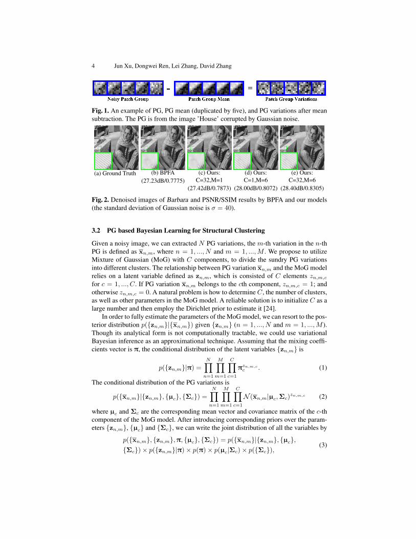
mean subtracted patch vector is xm = xm − µ. The X , {xm}, m = 1, ...,M iscalled the PG variations. In Figure 1, we show one example of PG, PG mean, and thePG variations after group mean subtraction. The PG mean is the main structure of thisPG. Here, we proposed to embed this idea into the BPFA model [27] and compare theperformance on the Gaussian noise removal. The results are listed in Figure 2. Whencomparing the images (b) and (d), we can see that the introduce of PG based NSSprior can really boost the performance on image denoising of the BPFA model. Theimprovements on PSNR is nearly 0.8dB and on SSIM is nearly 0.03. In particular, theimage quality in (d) is much better than that in (b).


Fig. 1. An example of PG, PG mean (duplicated by five), and PG variations after meansubtraction. The PG is from the image ’House’ corrupted by Gaussian noise.

(a) Ground Truth (b) BPFA(27.23dB/0.7775)

(c) Ours:C=32,M=1

(27.42dB/0.7873)

(d) Ours:C=1,M=6

(28.00dB/0.8072)

(e) Ours:C=32,M=6

(28.40dB/0.8305)

Fig. 2. Denoised images of Barbara and PSNR/SSIM results by BPFA and our models(the standard deviation of Gaussian noise is σ = 40).

3.2 PG based Bayesian Learning for Structural Clustering

Given a noisy image, we can extracted N PG variations, the m-th variation in the n-thPG is defined as xn,m, where n = 1, ..., N and m = 1, ...,M . We propose to utilizeMixture of Gaussian (MoG) with C components, to divide the sundry PG variationsinto different clusters. The relationship between PG variation xn,m and the MoG modelrelies on a latent variable defined as zn,m, which is consisted of C elements zn,m,c

for c = 1, ..., C. If PG variation xn,m belongs to the cth component, zn,m,c = 1; andotherwise zn,m,c = 0. A natural problem is how to determineC, the number of clusters,as well as other parameters in the MoG model. A reliable solution is to initialize C as alarge number and then employ the Dirichlet prior to estimate it [24].

In order to fully estimate the parameters of the MoG model, we can resort to the pos-terior distribution p({zn,m}|{xn,m}) given {zn,m} (n = 1, ..., N and m = 1, ...,M ).Though its analytical form is not computationally tractable, we could use variationalBayesian inference as an approximational technique. Assuming that the mixing coeffi-cients vector is π, the conditional distribution of the latent variables {zn,m} is

p({zn,m}|π) =N∏

n=1

M∏m=1

C∏c=1

πzn,m,cc . (1)

The conditional distribution of the PG variations is

p({xn,m}|{zn,m}, {µc}, {Σc}) =N∏

n=1

M∏m=1

C∏c=1

N (xn,m|µc,Σc)zn,m,c (2)

where µc and Σc are the corresponding mean vector and covariance matrix of the c-thcomponent of the MoG model. After introducing corresponding priors over the param-eters {zn,m}, {µc} and {Σc}, we can write the joint distribution of all the variables by

p({xn,m}, {zn,m},π, {µc}, {Σc}) = p({xn,m}|{zn,m}, {µc},{Σc})× p({zn,m}|π)× p(π)× p(µc|Σc)× p({Σc}),

(3)


where the mixing coefficients vector π is assumed to follow Dirichlet distribution.Finally, we can perform variational maximization (M step) and expectation esti-

matation of the responsibilities (E step) alternatively. By taking suitable parametersfor the equation 3, we can re-write the lower bound as a function of the parame-ters. This lower bound can be used to determine the posterior distribution over thenumber of components C in the MoG model. Please refer to [24] for more details.We use the Matlab code implemented in Pattern Recognition and Machine LearningToolbox http://www.mathworks.com/matlabcentral/fileexchange/55826-pattern-recognition-and-machine-learning-toolbox.

3.3 Discussion

Based on above description, we discuss as follows the advantages of the proposed modelfor PG based modeling directly on noisy images: Firstly, all the parameters of the pro-posed model are automatically estimated from the noisy image via variational Bayesianinference. This is a major advantage over PGPD [26]. Secondly, we demonstrated thatstructural clustering can indeed boost the performance of Bayesian methods such asBPFA [27]. This is demonstrated in the images (b) and (c) of Figure 2. Thirdly, theNon-local Self Similarity prior can be used to improve the performance of BPFA [27].This can be demonstrated by comparing the images ((b), (c), (e)) or ((b), (d), (e)).

4 Patch Group based Bayesian Dictionary Learning

4.1 Truncated beta-Bernoulli Process for Dictionary LearningOnce we have clustered similar PG variations into different components, we can extractthe latent clean PG variations using sparse or low rank image priors. These priors arealso frequently employed by many state-of-the-art methods [5–7, 25, 30, 26] for imagerestoration tasks. We do not fixed the number of atoms in the dictionary learning. Thisis different from the previous methods, including PGPD. Instead, we set a large numberK, which makes our Bayesian model a truncated beta-Bernoulli process. We employthe beta-Bernoulli process [20–22] to seek the sparse priors on infinite feature space.

In this paper, we express noisy PG variations X asX = DW + V, (4)

where X ∈ Rp2×M , the coefficients vector W ∈ RK×M , and the noise term V ∈Rp2×M . The matrix D ∈ Rp2×K contains K dictionary atoms. The coefficients matrixW is represented by W = B � S. The matrices B,S ∈ RK×M are the binary matrixand the coefficients matrix, respectively and � is the element-wise product. We denotex as any column of the PG variations X and w,b ∈ {0, 1}K , and s as correspondingcolumns of the coefficients matrix W, the binary matrix B, and the coefficients matrixS. We denote {dk}Kj=1 as columns of the dictionary D, {sj}nj=1 as columns of S, and{vj}nj=1 as columns of the noise matrix V. Each column w is represented by a binaryvector b ∈ {0, 1}K and a coefficient vector s ∈ RK×1, i.e., w = b � s. Then we canimpose suitable priors on these parameters, i.e., b, {dk}Kk=1, {sk}Kk=1, and {vj}nj=1.The binary vector b ∈ {0, 1}K denotes which of the columns (or atoms) in D areused for the representation of x. At beginning, we do not know the suitable K. Wecan set K → ∞ and impose sparse prior on b ∈ {0, 1}K to limit the number of


atoms in D used for representing each PG variation x extracted from noisy images.The beta-Bernoulli process [20–22] provides a convenient way for this purpose. Forinference convenience, we impose independent Gaussian priors on {dk}Kk=1, {sk}Kk=1,and {vj}nj=1.

The dictionary learning model for PG variations isX = DW + V,W = B� S, (5)

where � is element-wise product. The beta-Bernoulli process [22] for binary vector is:

b ∼K∏

k=1

Bernoulli(πk),π ∼K∏

k=1

Beta(a

K,b(K − 1)

K), (6)

dk ∼ N (0, P−1IP ), sj ∼ N (0, γ−1s IK),vj ∼ N (0, γ−1

v IP ), (7)γs ∼ Gamma(c, d), γv ∼ Gamma(e, f), (8)

where {a, b}, {c, d}, {e, f} are the corresponding hyper parameters of the parametersπ, γs, and γv in the conjugate hyper priors in equations (6), (8). The inference proce-dures we take for the Bayesian model is Gibbs sampling [31] and we ignore the pro-cedures here. As we can see, the noise estimation is integrated into the overall modelin Gibbs samppling process. That is th reason why the proposed algorithm can be usedto deal with blind noise. This is also different from the other non-blind image denois-ing methods [2, 5–7, 25, 30, 26], since they do not have the ability to estimate the noisewithin the noisy images.

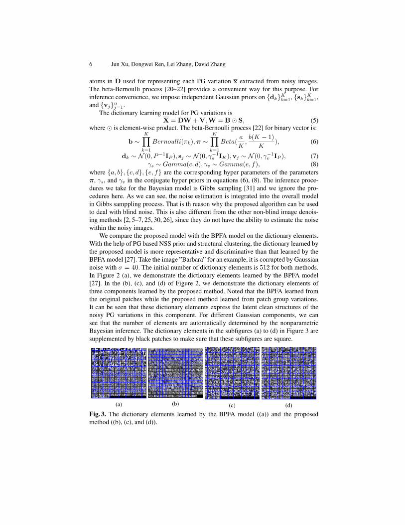
We compare the proposed model with the BPFA model on the dictionary elements.With the help of PG based NSS prior and structural clustering, the dictionary learned bythe proposed model is more representative and discriminative than that learned by theBPFA model [27]. Take the image ”Barbara” for an example, it is corrupted by Gaussiannoise with σ = 40. The initial number of dictionary elements is 512 for both methods.In Figure 2 (a), we demonstrate the dictionary elements learned by the BPFA model[27]. In the (b), (c), and (d) of Figure 2, we demonstrate the dictionary elements ofthree components learned by the proposed method. Noted that the BPFA learned fromthe original patches while the proposed method learned from patch group variations.It can be seen that these dictionary elements express the latent clean structures of thenoisy PG variations in this component. For different Gaussian components, we cansee that the number of elements are automatically determined by the nonparametricBayesian inference. The dictionary elements in the subfigures (a) to (d) in Figure 3 aresupplemented by black patches to make sure that these subfigures are square.

(a) (b) (c) (d)

Fig. 3. The dictionary elements learned by the BPFA model ((a)) and the proposedmethod ((b), (c), and (d)).


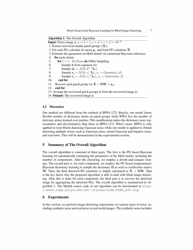
Algorithm 1: The Overall AlgorithmInput: Noisy image y, a = b = 1, c = d = e = f = 10−6

1. Extract non-local similar patch groups {X};2. For each PG, calculate its mean µx and form PG variations X;3. Estimate the parameters in MoG model via variational Bayesian inference;4. for each cluster5. for t = 1 : IteNum do Gibbs Sampling:6. Sample b from equation (6)7. Sample dk ∼ N (0, P−1IP )8. Sample sj ∼ N (0, γ−1

s IK , γs ∼ Gamma(c, d)9. Sample vj ∼ N (0, γ−1

v IP ), γv ∼ Gamma(e, f)10. end for11. Recover each patch group via X = DW + µx;12. end for13. Average the recovered patch groups to form the recovered image y;14. Output: The recovered image y.

4.2 Discussion

Our method are different from the method of BPFA [27]. Basicly, our model learnsflexible number of dictionary atoms on patch groups while BPFA fixs the number ofdictioary atoms learned over patches. This modification makes the dictionary more rep-resentative and discriminative than those in BPFA [27]. What’s more, BPFA is onlyapplied in (non-blind) denoising Gaussian noise while our model is applied to (blind)denoising multiple noises such as Gaussian noise, mixed Gaussian and impulse noise,and real noise. This will be demonstrated in the experimental section.

5 Summary of The Overall Algorithm

The overall algorithm is consisted of three parts. The first is the PG based Bayesianlearning for automatically estimating the parameters of the MoG model, including thenumber of components. After the clustering, we employ a divide-and-conquer strat-egy. The second part is, for each component, we employ the PG based nonparametricBayesian dictionary learning to sample the dictionary D as well as coefficients matrixW. Then, the final denoised PG variations is simply calculated as X = DW. Thatis the key factor why the proposed algorithm is able to deal with blind image denois-ing. After this is done for each component, the third part is to recover the denoisedimage by aggregating the denoised PGs. The overall algorithm is summarized in Al-gorithm 1. The Matlab source code of our algorithm can be downloaded at http://www4.comp.polyu.edu.hk/˜csjunxu/code/PGBL_BID.zip.

6 Experiments

In this section, we perform image denoising experiments on various types of noise, in-cluding synthetic noise and real noise in real world images. The synthetic noise includes


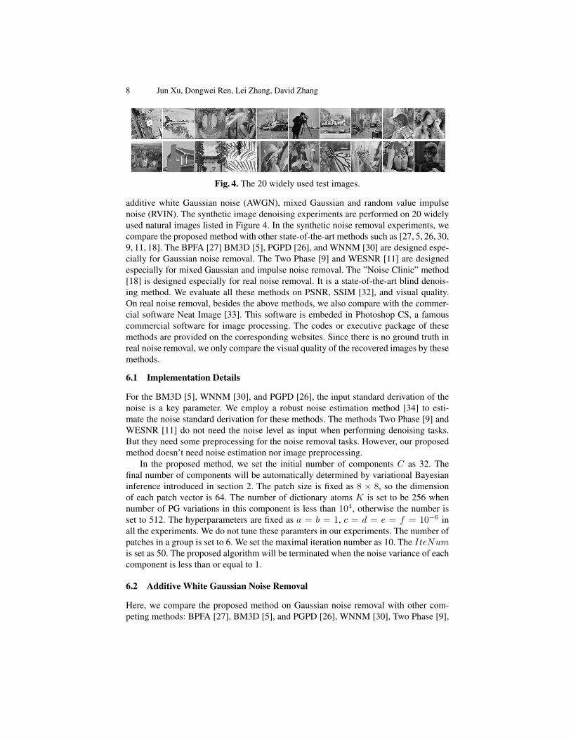
Fig. 4. The 20 widely used test images.

additive white Gaussian noise (AWGN), mixed Gaussian and random value impulsenoise (RVIN). The synthetic image denoising experiments are performed on 20 widelyused natural images listed in Figure 4. In the synthetic noise removal experiments, wecompare the proposed method with other state-of-the-art methods such as [27, 5, 26, 30,9, 11, 18]. The BPFA [27] BM3D [5], PGPD [26], and WNNM [30] are designed espe-cially for Gaussian noise removal. The Two Phase [9] and WESNR [11] are designedespecially for mixed Gaussian and impulse noise removal. The ”Noise Clinic” method[18] is designed especially for real noise removal. It is a state-of-the-art blind denois-ing method. We evaluate all these methods on PSNR, SSIM [32], and visual quality.On real noise removal, besides the above methods, we also compare with the commer-cial software Neat Image [33]. This software is embeded in Photoshop CS, a famouscommercial software for image processing. The codes or executive package of thesemethods are provided on the corresponding websites. Since there is no ground truth inreal noise removal, we only compare the visual quality of the recovered images by thesemethods.

6.1 Implementation Details

For the BM3D [5], WNNM [30], and PGPD [26], the input standard derivation of thenoise is a key parameter. We employ a robust noise estimation method [34] to esti-mate the noise standard derivation for these methods. The methods Two Phase [9] andWESNR [11] do not need the noise level as input when performing denoising tasks.But they need some preprocessing for the noise removal tasks. However, our proposedmethod doesn’t need noise estimation nor image preprocessing.

In the proposed method, we set the initial number of components C as 32. Thefinal number of components will be automatically determined by variational Bayesianinference introduced in section 2. The patch size is fixed as 8 × 8, so the dimensionof each patch vector is 64. The number of dictionary atoms K is set to be 256 whennumber of PG variations in this component is less than 104, otherwise the number isset to 512. The hyperparameters are fixed as a = b = 1, c = d = e = f = 10−6 inall the experiments. We do not tune these paramters in our experiments. The number ofpatches in a group is set to 6. We set the maximal iteration number as 10. The IteNumis set as 50. The proposed algorithm will be terminated when the noise variance of eachcomponent is less than or equal to 1.

6.2 Additive White Gaussian Noise Removal

Here, we compare the proposed method on Gaussian noise removal with other com-peting methods: BPFA [27], BM3D [5], and PGPD [26], WNNM [30], Two Phase [9],


WNSER [11], Noise Clinic [18]. As a common experimental setting, we add additivewhite Gaussian noise with zero mean and standard deviation σ to the test images. Thedenoising experiments are performed on multiple noise levels of σ = 30, 40, 50, 75.

The averaged results on PSNR and SSIM are listed in Tables 1 and 2. We can seethat the PSNR and SSIM results of our proposed method are much better than theBPFA, Two Phase, and WESNR, Noise Clinic methods. The results of the proposedmethod are comparable to BM3D when the noise levels are higher than 30. Thoughgetting inferior results on PSNR and SSIM when compared to WNNM and PGPD, theproposed method can achieve similar or even better performance when compared withother methods. For instance, from Figure 4 and Figure 5, we can see that the proposedmethod generates better image quality and less artifacts on the image ”House” and”Hill” than the other methods. Considering that the proposed method is fully blind, it ismore convincing to see that our proposed method achieves better image quality resultsthan the Noise Clinic [18], which is a state-of-the-art blind image denoising method.We want to mention again that BM3D, PGPD, and WNNM can only work well on theGaussian noise, which they are designed for, but perform poorly on other types of noise,which will be demonstrated later.

Table 1. Average PSNR(dB) results of different algorithms on 20 natural images cor-rupted by Gaussian noise.

σ BPFA BM3D WNNM PGPD Two Phase WESNR Noise Clinic Ours30 28.81 29.11 29.35 29.13 18.84 27.44 26.81 28.6540 27.45 27.68 28.03 27.88 16.52 25.07 24.90 27.5950 26.38 26.80 27.06 26.89 14.80 22.02 23.47 26.6875 24.40 25.04 25.25 25.11 11.95 9.02 21.31 24.91

Table 2. Average SSIM results of different algorithms on 20 natural images corruptedby Gaussian noise.

σ BPFA BM3D WNNM PGPD Two Phase WESNR Noise Clinic Ours30 0.7988 0.8108 0.8156 0.8089 0.3137 0.7430 0.6520 0.797140 0.7576 0.7706 0.7784 0.7747 0.2361 0.6063 0.5631 0.766850 0.7216 0.7430 0.7510 0.7435 0.1855 0.4483 0.4990 0.738275 0.6470 0.6803 0.6897 0.6825 0.1147 0.1749 0.4289 0.6766

6.3 Mixed Gaussian and Impulse Noise Removal

Here, we compare the proposed method on mixed Gaussian and impulse noise with thecompared methods [27, 5, 26, 30, 9, 11, 18]. We consider Random Value Impulse Noise(RVIN) here. The pixels in the testing image corrupted by RVIN is distributed between0 and 255. This is much harder than salt and pepper noise, which is only 0 or 255 values.In the synthetic noise, the standard derivations of the Gaussian noise are σ = 10, 20 andthe ratios of the impulse noise are 0.15, 0.30, respectively. The RVIN noise is generatedby the ”impulsenoise” function used by WESNR [11].


(a) Ground Truth (b) Noisy Image(16.30dB/0.1701)

(c) BPFA(29.75dB/0.8048)

(d) BM3D(30.63dB/0.8231)

(e) PGPD(31.02dB/0.8302)

(f) WNNM(31.19dB/0.8279)

(g) Two Phase(16.30dB/0.1701)

(h) WESNR(27.27dB/0.6076)

(i) Noise Clinic(26.48dB/0.5370)

(j) Ours(30.90dB/0.8328)

Fig. 5. Denoised images of House and PSNR/SSIM results by different methods (thestandard deviation of Gaussian noise is σ = 40).


(c) BPFA(26.81dB/0.6530)

(d) BM3D(27.19dB/0.6745)

(e) PGPD(27.22dB/0.6702)

(f) WNNM(27.34dB/0.6772)

(g) Two Phase(14.68dB/0.1357)

(h) WESNR(23.50dB/0.4218)


(j) Ours(27.02dB/0.6618)

Fig. 6. Denoised images of Hill and PSNR/SSIM results by different methods (the stan-dard deviation of Gaussian noise is σ = 50).


For BPFA [27], BM3D [5], and PGPD [26], WNNM [30], they are designed todeal with Gaussian noise. Hence, we still employ the noise estimation method [34]to estimate the noise levels σ. We also compare the proposed method with the methodsTwo Phase [9] and WESNR [11], which are designed especially for the mixed Gaussianand RVIN noise. Noted that both Two Phase [9] and WESNR [11] employ AdaptiveMedian Filter (AMF) [35] to preprocess the image before performing image denoisingtask. We also compare with the Noise Clinic [18].

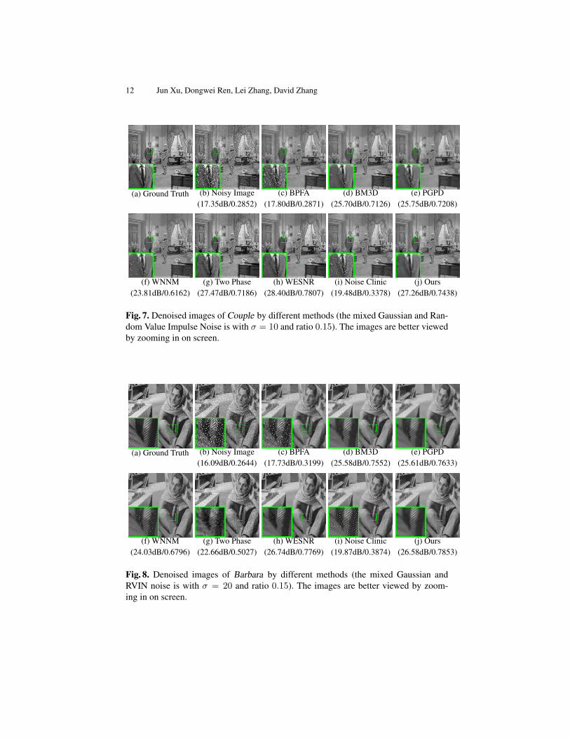
The results on PSNR and SSIM are listed in Table 3 and Table 4. As we can see,the performance of the proposed method is comparable or better than other methods.For the visual quality comparison, the proposed method can generate better results thanother methods. Take the image ”Couple” for an example, from the Figure 7, the pro-posed method removes the noise clearly while all other methods remain some noiseor generate some artifacts. From the results on ”Barbara” listed in Figure 8, the pro-posed method achieves higher SSIM and generates better image quality than all othermethods. We have to mention again that the Two Phase and WESNR are two state-of-the-art methods designed especially for the mixed Gaussian and impulse noise. But theyperform poorly on other types of noises such as Gaussian.

Table 3. Average PSNR(dB) results of different algorithms on 20 natural images cor-rupted by mixed of Gaussian and RVIN noise.

σ, Ratio BPFA BM3D WNNM PGPD Two Phase WESNR Noise Clinic Ours10, 0.15 17.12 25.18 22.98 25.41 27.28 27.37 18.66 27.1710, 0.30 14.19 21.80 21.40 21.74 26.12 21.50 16.44 22.1720, 0.15 17.62 25.13 23.57 25.33 24.43 27.24 19.66 26.1220, 0.30 17.61 21.73 21.40 21.64 23.61 22.69 14.46 21.89

Table 4. Average SSIM results of different algorithms on 20 natural images corruptedby mixed of Gaussian and RVIN noise.

σ, Ratio BPFA BM3D WNNM PGPD Two Phase WESNR Noise Clinic Ours10, 0.15 0.2749 0.7037 0.5806 0.7242 0.7091 0.7499 0.3198 0.745910, 0.30 0.1576 0.6444 0.6038 0.6405 0.6783 0.4970 0.2042 0.655920, 0.15 0.2821 0.7132 0.6190 0.7220 0.5468 0.7568 0.3423 0.731220, 0.30 0.2821 0.6414 0.6310 0.6371 0.5183 0.5871 0.1346 0.6470

6.4 Real Noisy Image DenoisingIn this section, we will test the proposed method on real noise removal. Since thecolor images are in RGB channels, we firstly transform the color images into YCbCrchannels, then perfrom denoising on the Y channel, and finally transform the denoisedYCbCr channel image back into RGB channels. The denoised images are cropped tosize of 800 × 600 for better visualization. We do not compare with WNNM [30] andTwo Phase [9] here since they achieve worse denoising quality than the other methodssuch as BM3D [5], WESNR [11], and Noise Clinic [18]. For BM3D and PGPD, theinput noise level σ is still estimated by [34]. We also compare with the Neat Image[33], a commercial software embedded in Photoshop CS. In this paper, we take threereal noisy images for examples, which are ”SolvayConf1927”, ”Girls”, and ”Windmill”.The image ”SolvayConf1927” is an old image provided by the Noise Clinic website on



(c) BPFA(17.80dB/0.2871)

(d) BM3D(25.70dB/0.7126)

(e) PGPD(25.75dB/0.7208)

(f) WNNM(23.81dB/0.6162)

(g) Two Phase(27.47dB/0.7186)

(h) WESNR(28.40dB/0.7807)


(j) Ours(27.26dB/0.7438)

Fig. 7. Denoised images of Couple by different methods (the mixed Gaussian and Ran-dom Value Impulse Noise is with σ = 10 and ratio 0.15). The images are better viewedby zooming in on screen.


(c) BPFA(17.73dB/0.3199)

(d) BM3D(25.58dB/0.7552)

(e) PGPD(25.61dB/0.7633)

(f) WNNM(24.03dB/0.6796)

(g) Two Phase(22.66dB/0.5027)

(h) WESNR(26.74dB/0.7769)


(j) Ours(26.58dB/0.7853)

Fig. 8. Denoised images of Barbara by different methods (the mixed Gaussian andRVIN noise is with σ = 20 and ratio 0.15). The images are better viewed by zoom-ing in on screen.


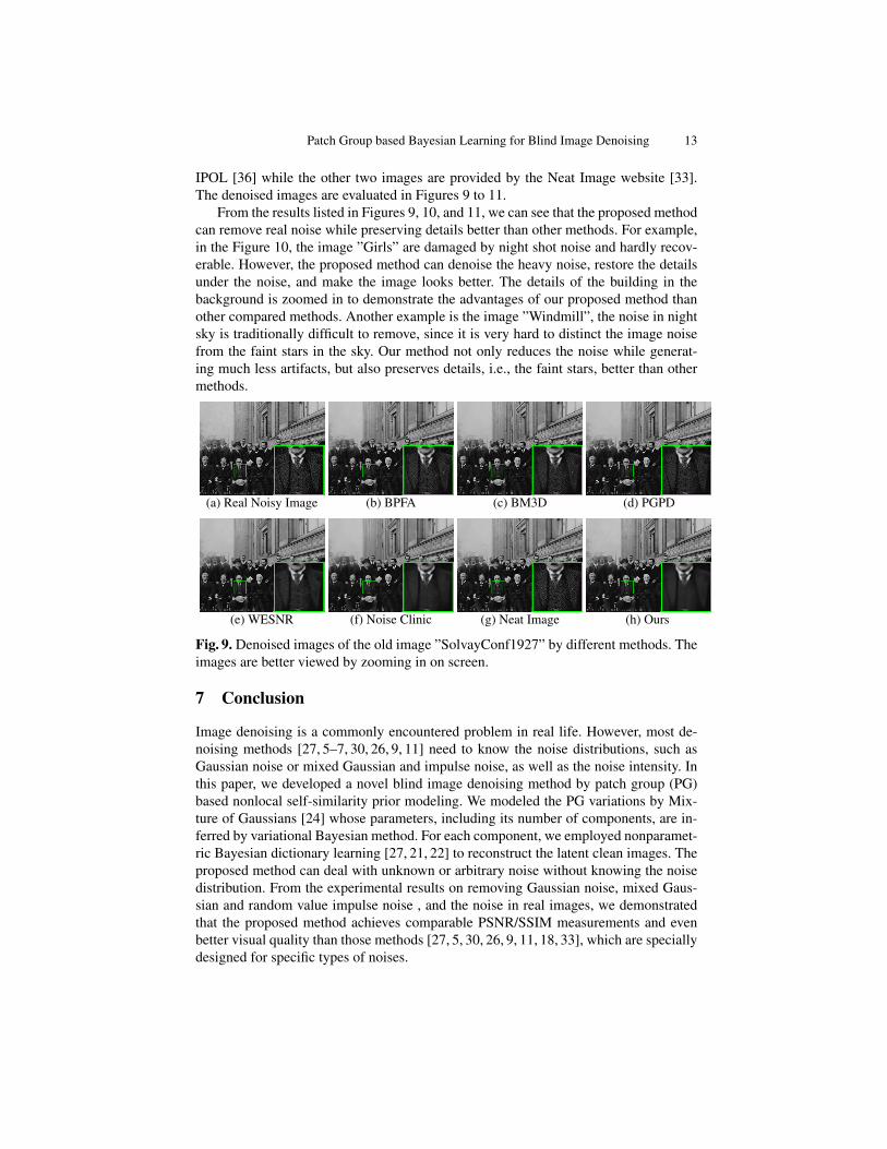
IPOL [36] while the other two images are provided by the Neat Image website [33].The denoised images are evaluated in Figures 9 to 11.

From the results listed in Figures 9, 10, and 11, we can see that the proposed methodcan remove real noise while preserving details better than other methods. For example,in the Figure 10, the image ”Girls” are damaged by night shot noise and hardly recov-erable. However, the proposed method can denoise the heavy noise, restore the detailsunder the noise, and make the image looks better. The details of the building in thebackground is zoomed in to demonstrate the advantages of our proposed method thanother compared methods. Another example is the image ”Windmill”, the noise in nightsky is traditionally difficult to remove, since it is very hard to distinct the image noisefrom the faint stars in the sky. Our method not only reduces the noise while generat-ing much less artifacts, but also preserves details, i.e., the faint stars, better than othermethods.

(a) Real Noisy Image (b) BPFA (c) BM3D (d) PGPD

(e) WESNR (f) Noise Clinic (g) Neat Image (h) Ours

Fig. 9. Denoised images of the old image ”SolvayConf1927” by different methods. Theimages are better viewed by zooming in on screen.

7 Conclusion

Image denoising is a commonly encountered problem in real life. However, most de-noising methods [27, 5–7, 30, 26, 9, 11] need to know the noise distributions, such asGaussian noise or mixed Gaussian and impulse noise, as well as the noise intensity. Inthis paper, we developed a novel blind image denoising method by patch group (PG)based nonlocal self-similarity prior modeling. We modeled the PG variations by Mix-ture of Gaussians [24] whose parameters, including its number of components, are in-ferred by variational Bayesian method. For each component, we employed nonparamet-ric Bayesian dictionary learning [27, 21, 22] to reconstruct the latent clean images. Theproposed method can deal with unknown or arbitrary noise without knowing the noisedistribution. From the experimental results on removing Gaussian noise, mixed Gaus-sian and random value impulse noise , and the noise in real images, we demonstratedthat the proposed method achieves comparable PSNR/SSIM measurements and evenbetter visual quality than those methods [27, 5, 30, 26, 9, 11, 18, 33], which are speciallydesigned for specific types of noises.



(e) WESNR (f) Noise Clinic (g) Neat Image (h) Ours

Fig. 10. Denoised images of the image ”Girls” by different methods. The images arebetter viewed by zooming in on screen.


(c) WESNR (d) Noise Clinic (e) Neat Image (f) Ours

Fig. 11. Photo courtesy of Alexander Semenov. Denoised images of the image ”Wind-mill” by different methods. The images are better viewed by zooming in on screen.


References

1. Rudin, L.I., Osher, S., Fatemi, E.: Nonlinear total variation based noise removal algorithms.Physica D: Nonlinear Phenomena 60 (1992) 259–268

2. Buades, A., Coll, B., Morel, J.M.: A non-local algorithm for image denoising. CVPR (2005)60–65

3. Roth, S., Black, M.J.: Fields of Experts. International Journal of Computer Vision 82 (2009)205–229

4. Elad, M., Aharon, M.: Image denoising via sparse and redundant representations over learneddictionaries. Image Processing, IEEE Transactions on 15 (2006) 3736–3745

5. Dabov, K., Foi, A., Katkovnik, V., Egiazarian, K.: Image denoising by sparse 3-D transform-domain collaborative filtering. Image Processing, IEEE Transactions on 16 (2007) 2080–2095

6. Mairal, J., Bach, F., Ponce, J., Sapiro, G., Zisserman, A.: Non-local sparse models for imagerestoration. ICCV (2009) 2272–2279

7. Zoran, D., Weiss, Y.: From learning models of natural image patches to whole image restora-tion. ICCV (2011) 479–486

8. Burger, H.C., Schuler, C.J., Harmeling, S.: Image denoising: Can plain neural networkscompete with bm3d? In: Computer Vision and Pattern Recognition (CVPR), 2012 IEEEConference on, IEEE (2012) 2392–2399

9. Cai, J.F., Chan, R.H., Nikolova, M.: Fast two-phase image deblurring under impulse noise.Journal of Mathematical Imaging and Vision 36 (2010) 46–53

10. Xiao, Y., Zeng, T., Yu, J., Ng, M.K.: Restoration of images corrupted by mixed gaussian-impulse noise via l1l0 minimization. Pattern Recognition 44 (2011) 1708 – 1720

11. Jiang, J., Zhang, L., Yang, J.: Mixed noise removal by weighted encoding with sparse non-local regularization. Image Processing, IEEE Transactions on 23 (2014) 2651–2662

12. Portilla, J., Strela, V., Wainwright, M., Simoncelli, E.: Image denoising using scale mixturesof Gaussians in the wavelet domain. Image Processing, IEEE Transactions on 12 (2003)1338–1351

13. Portilla, J.: Full blind denoising through noise covariance estimation using gaussian scalemixtures in the wavelet domain. Image Processing, 2004. ICIP ’04. 2004 International Con-ference on 2 (2004) 1217–1220

14. Huber, P.J.: Robust statistics. Springer (2011)15. Rabie, T.: Robust estimation approach for blind denoising. Image Processing, IEEE Trans-

actions on 14 (2005) 1755–176516. Liu, C., Szeliski, R., Kang, S.B., Zitnick, C.L., Freeman, W.T.: Automatic estimation and

removal of noise from a single image. IEEE Transactions on Pattern Analysis and MachineIntelligence 30 (2008) 299–314

17. Gong, Z., Shen, Z., Toh, K.C.: Image restoration with mixed or unknown noises. MultiscaleModeling & Simulation 12 (2014) 458–487

18. Lebrun, M., Colom, M., Morel, J.M.: Multiscale image blind denoising. Image Processing,IEEE Transactions on 24 (2015) 3149–3161

19. Lebrun, M., Buades, A., Morel, J.M.: A nonlocal bayesian image denoising algorithm. SIAMJournal on Imaging Sciences 6 (2013) 1665–1688

20. Hjort, N.L.: Nonparametric bayes estimators based on beta processes in models for lifehistory data. The Annals of Statistics (1990) 1259–1294

21. Thibaux, R., Jordan, M.I.: Hierarchical beta processes and the indian buffet process. In:International conference on artificial intelligence and statistics. (2007) 564–571

22. Paisley, J., Carin, L.: Nonparametric factor analysis with beta process priors. In: Proceedingsof the 26th Annual International Conference on Machine Learning, ACM (2009) 777–784


23. Yu, G., Sapiro, G., Mallat, S.: Solving inverse problems with piecewise linear estimators:From Gaussian mixture models to structured sparsity. Image Processing, IEEE Transactionson 21 (2012) 2481–2499

24. Bishop, C.M.: Pattern recognition and machine learning. (2006)25. Dong, W., Zhang, L., Shi, G., Li, X.: Nonlocally centralized sparse representation for image

restoration. Image Processing, IEEE Transactions on 22 (2013) 1620–163026. Xu, J., Zhang, L., Zuo, W., Zhang, D., Feng, X.: Patch group based nonlocal self-similarity

prior learning for image denoising. The IEEE International Conference on Computer Vision(ICCV) (2015) 244–252

27. Zhou, M., Chen, H., Ren, L., Sapiro, G., Carin, L., Paisley, J.W.: Non-parametric bayesiandictionary learning for sparse image representations. In: NIPS. (2009) 2295–2303

28. Ferguson, T.S.: A bayesian analysis of some nonparametric problems. The annals of statistics(1973) 209–230

29. Ren, L., Du, L., Carin, L., Dunson, D.: Logistic stick-breaking process. The Journal ofMachine Learning Research 12 (2011) 203–239

30. Gu, S., Zhang, L., Zuo, W., Feng, X.: Weighted nuclear norm minimization with applicationto image denoising. CVPR (2014) 2862–2869

31. Zhou, M., Chen, H., Paisley, J., Ren, L., Li, L., Xing, Z., Dunson, D., Sapiro, G., Carin, L.:Nonparametric bayesian dictionary learning for analysis of noisy and incomplete images.Image Processing, IEEE Transactions on 21 (2012) 130–144

32. Wang, Z., Bovik, A.C., Sheikh, H.R., Simoncelli, E.P.: Image quality assessment: from errorvisibility to structural similarity. Image Processing, IEEE Transactions on 13 (2004) 600–612

33. ABSoft, N.: Neat image. (https://ni.neatvideo.com/home)34. Liu, X., Tanaka, M., Okutomi, M.: Single-image noise level estimation for blind denoising.

Image Processing, IEEE Transactions on 22 (2013) 5226–523735. Hwang, H., Haddad, R.: Adaptive median filters: new algorithms and results. Image Pro-

cessing, IEEE Transactions on 4 (1995) 499–50236. Lebrun, M., Colom, M., Morel, J.M.: The noise clinic: a blind image denoising algorithm.

(http://www.ipol.im/pub/art/2015/125/) Accessed 01 28, 2015.

Patch Group based Bayesian Learning for Blind Image Denoisingcsjunxu/paper/PGBL_BID.pdf ·...

Documents

Transcript of Patch Group based Bayesian Learning for Blind Image Denoisingcsjunxu/paper/PGBL_BID.pdf ·...