Partitioning a Graph in Alliances and its Application to...

Partitioning a Graph in Alliances and its Application to DataClustering

by

Khurram Hassan ShafiqueB.E. (Computer Systems Engineering)

N.E.D. University of Engineering and TechnologyM.Sc. (Computer Science)

University of Central Florida

A dissertation submitted in partial fulfillment of the requirementsfor the degree of Doctor of Philosophy

in the School of Computer Sciencein the College of Engineering and Computer Science

at the University of Central FloridaOrlando, Florida

Fall Term2004

Major Professor:Ronald D. Dutton

UMI Number: 3163605

31636052005

UMI MicroformCopyright

All rights reserved. This microform edition is protected against unauthorized copying under Title 17, United States Code.

ProQuest Information and Learning Company 300 North Zeeb Road

P.O. Box 1346 Ann Arbor, MI 48106-1346

by ProQuest Information and Learning Company.

Abstract

Any reasonably large group of individuals, families, states, and parties exhibits the phe-

nomenon of subgroup formations within the group such that the members of each group

have a strong connection or bonding between each other. The reasons of the formation

of these subgroups that we call alliances differ in different situations, such as, kinship and

friendship (in the case of individuals), common economic interests (for both individuals and

states), common political interests, and geographical proximity. This structure of alliances is

not only prevalent in social networks, but it is also an important characteristic of similarity

networks of natural and unnatural objects. (A similarity network defines the links between

two objects based on their similarities). Discovery of such structure in a data set is called

clustering or unsupervised learning and the ability to do it automatically is desirable for

many applications in the areas of pattern recognition, computer vision, artificial intelligence,

behavioral and social sciences, life sciences, earth sciences, medicine, and information theory.

In this dissertation, we study a graph theoretical model of alliances where an alliance of

the vertices of a graph is a set of vertices in the graph, such that every vertex in the set

is adjacent to equal or more vertices inside the set than the vertices outside it. We study

the problem of partitioning a graph into alliances and identify classes of graphs that have

such a partition. We present results on the relationship between the existence of such a

iii

partition and other well known graph parameters, such as connectivity, subgraph structure,

and degrees of vertices. We also present results on the computational complexity of finding

such a partition.

An alliance cover set is a set of vertices in a graph that contains at least one vertex from

every alliance of the graph. The complement of an alliance cover set is an alliance free set,

that is, a set that does not contain any alliance as a subset. We study the properties of

these sets and present tight bounds on their cardinalities. In addition, we also characterize

the graphs that can be partitioned into alliance free and alliance cover sets.

Finally, we present an approximate algorithm to discover alliances in a given graph. At

each step, the algorithm finds a partition of the vertices into two alliances such that the

alliances are strongest among all such partitions. The strength of an alliance is defined as

a real number p, such that every vertex in the alliance has at least p times more neighbors

in the set than its total number of neighbors in the graph). We evaluate the performance of

the proposed algorithm on standard data sets.

iv

Dedicated to my daughter Aleesha

v

Acknowledgments

I would first like to thank my thesis advisor, Professor Ronald D. Dutton, who introduced

me to the fields of graph theory, computational complexity and algorithms.

Special thanks to Professor Mubarak Shah for his support and encouragement during my

studies.

It is also a pleasure to thank Professor Robert Brigham, Professor Narsingh Deo, Pro-

fessor David Workman, and Professor Yue Zhao for serving as my committee members and

for their valuable comments and suggestions.

Finally I thank my wife, Wajiha Khurram, my sister, Huma Shafique, my parents Rehana

Shafique and M. Shafique Siddiqui, for their patience, and understanding during the entire

period of my tenure as a graduate student.

vi

Table of Contents

LIST OF TABLES . . . . . . . . . . . . . . . . . . . . . . . . . . . . . . . . . . . x

LIST OF FIGURES . . . . . . . . . . . . . . . . . . . . . . . . . . . . . . . . . . xi

CHAPTER 1 INTRODUCTION . . . . . . . . . . . . . . . . . . . . . . . . . . 1

1.1 Motivation . . . . . . . . . . . . . . . . . . . . . . . . . . . . . . . . . . . . . 1

1.2 Definitions and Notation . . . . . . . . . . . . . . . . . . . . . . . . . . . . . 5

1.3 Dissertation Outline . . . . . . . . . . . . . . . . . . . . . . . . . . . . . . . 7

CHAPTER 2 ALLIANCES IN GRAPHS . . . . . . . . . . . . . . . . . . . . 8

2.1 Introduction . . . . . . . . . . . . . . . . . . . . . . . . . . . . . . . . . . . . 8

2.2 Types of Alliances . . . . . . . . . . . . . . . . . . . . . . . . . . . . . . . . 11

2.3 Alliance Numbers . . . . . . . . . . . . . . . . . . . . . . . . . . . . . . . . . 13

2.4 Basic Properties and Known Bounds on Alliance Numbers . . . . . . . . . . 16

2.4.1 Defensive Alliance Numbers . . . . . . . . . . . . . . . . . . . . . . . 16

2.4.2 Global Defensive Alliance Numbers . . . . . . . . . . . . . . . . . . . 20

2.4.3 Offensive Alliance Numbers . . . . . . . . . . . . . . . . . . . . . . . 21

vii

2.4.4 Powerful Alliance Numbers . . . . . . . . . . . . . . . . . . . . . . . . 22

2.5 Open Problems . . . . . . . . . . . . . . . . . . . . . . . . . . . . . . . . . . 31

CHAPTER 3 PARTITIONING A GRAPH INTO DEFENSIVE AND GLOBAL

DEFENSIVE ALLIANCES . . . . . . . . . . . . . . . . . . . . . . . . . . . . . . 34

3.1 Introduction . . . . . . . . . . . . . . . . . . . . . . . . . . . . . . . . . . . . 34

3.2 Basic Properties . . . . . . . . . . . . . . . . . . . . . . . . . . . . . . . . . . 38

3.3 Satisfiability and Connectivity . . . . . . . . . . . . . . . . . . . . . . . . . . 41

3.4 Subgraph Characterizations . . . . . . . . . . . . . . . . . . . . . . . . . . . 44

3.5 Satisfiability and Cardinality of Minimum Alliance . . . . . . . . . . . . . . 46

3.6 Special Cases . . . . . . . . . . . . . . . . . . . . . . . . . . . . . . . . . . . 48

3.6.1 Satisfiability of Regular Graphs . . . . . . . . . . . . . . . . . . . . . 49

3.6.2 Satisfiability of Odd Graphs and Triangle free Eulerian Graphs . . . . 55

3.6.3 Satisfiability of Line Graphs . . . . . . . . . . . . . . . . . . . . . . . 57

3.7 Computational Complexity . . . . . . . . . . . . . . . . . . . . . . . . . . . . 63

CHAPTER 4 ALLIANCE FREE AND ALLIANCE COVER SETS . . . 67

4.1 Introduction . . . . . . . . . . . . . . . . . . . . . . . . . . . . . . . . . . . . 67

4.2 Basic Properties . . . . . . . . . . . . . . . . . . . . . . . . . . . . . . . . . . 69

4.3 Defensive k−Alliance Free & Cover Sets . . . . . . . . . . . . . . . . . . . . 71

viii

4.4 Offensive k−Alliance Free & Cover Sets . . . . . . . . . . . . . . . . . . . . . 80

CHAPTER 5 PARTITIONING A GRAPH INTO DEFENSIVE 0-ALLIANCE

FREE (COVER) SETS . . . . . . . . . . . . . . . . . . . . . . . . . . . . . . . . . 84

5.1 When G is not Partitionable . . . . . . . . . . . . . . . . . . . . . . . . . . . 85

5.2 When a Block is Not Partitionable . . . . . . . . . . . . . . . . . . . . . . . 88

CHAPTER 6 GRAPH PARTITIONING AND DATA CLUSTERING . . 93

6.1 Introduction . . . . . . . . . . . . . . . . . . . . . . . . . . . . . . . . . . . . 93

6.2 Graph Theoretical Techniques for Clustering . . . . . . . . . . . . . . . . . . 100

6.3 Clustering Using Maximum Satisfactory Minimum Cut . . . . . . . . . . . . 106

6.3.1 Problem Definition . . . . . . . . . . . . . . . . . . . . . . . . . . . . 106

6.3.2 Semidefinite Relaxation of MSMC . . . . . . . . . . . . . . . . . . . . 110

6.4 Results . . . . . . . . . . . . . . . . . . . . . . . . . . . . . . . . . . . . . . . 115

6.4.1 Zachary’s Karate Club Network . . . . . . . . . . . . . . . . . . . . . 115

6.4.2 Zoo Database . . . . . . . . . . . . . . . . . . . . . . . . . . . . . . . 116

6.4.3 Networks of Fictional Characters . . . . . . . . . . . . . . . . . . . . 121

6.4.4 Other Standard Data Sets . . . . . . . . . . . . . . . . . . . . . . . . 122

6.5 Conclusion . . . . . . . . . . . . . . . . . . . . . . . . . . . . . . . . . . . . . 131

REFERENCES . . . . . . . . . . . . . . . . . . . . . . . . . . . . . . . . . . . . 134

ix

List of Tables

6.1 General Information about Zoo database. . . . . . . . . . . . . . . . . . . . . . 119

6.2 Clusters of animals in the Zoo database as found by the proposed algorithm. . . . 120

6.3 Grouping of characters of Victor Hugo’s Les Miserables. . . . . . . . . . . . . . . 123

6.4 General information about Wine Recognition database. . . . . . . . . . . . . . . 126

6.5 General information about Iris Plant data set . . . . . . . . . . . . . . . . . . . 126

6.6 General information about Hepatitis data set . . . . . . . . . . . . . . . . . . . 127

6.7 General information about Dermatology data set . . . . . . . . . . . . . . . . . 127

6.8 General information about Protein Localization Sites (Ecoli) data set . . . . . . . 130

6.9 Comparison of MSMC Algorithm and Normalized Cut Algorithm . . . . . . . . . 132

x

List of Figures

2.1 (a) An 11-vertex component (b)A 9-vertex component.(c) Constructed graph G′.

Each vertex vi, 1 ≤ i ≤ K is connected to an 11-vertex component and each vertex

vj , K + 1 ≤ j ≤ n, is connected to a 9-vertex component. . . . . . . . . . . . . . 25

2.2 (a) Construction of an instance of PA from an instance of AHGPA. . . . . . . . . 27

6.1 (a) Two levels of a clustering hierarchy. In the first level the graph is split into two

clusters A and B. In the second level, each of these clusters are further subdivided

into two clusters. (b) Three levels of a clustering hierarchy. In the first level the

graph is split into two clusters A and B. In the second level, cluster A is again split

into two clusters A1 and A2. Cluster A1 is split into two more clusters in level 3. . 98

6.2 The dendrograms (or hierarchical trees) of the hierarchies shown in Figure 6.1. The

leaves of the dendrogram represent the final clusters. As we move up the tree, the

vertices join together to form larger and larger clusters (indicated by horizontal

lines). All these clusters are joined together in a single group at the root of the tree. 99

xi

6.3 The network of ties between the members of the karate club from Zachary Karate

Club data set. The bipartition of the data generated by our algorithm is shown by

using different colors for the members belonging to different clusters. The members

with greater ties with the administrator (vertex 1) are colored blue whereas the

members with greater ties with the instructor (vertex 33) are colored yellow. Only

the coloring of vertex 3 is inconsistent with the actual split of the club. . . . . . 116

6.4 Final clustering of the Zachary Karate Club data generated by the proposed algo-

rithm. . . . . . . . . . . . . . . . . . . . . . . . . . . . . . . . . . . . . . . . 117

6.5 Grouping among the animals of zoo database. A total of 9 groups were recognized

by the algorithm. . . . . . . . . . . . . . . . . . . . . . . . . . . . . . . . . . . 118

6.6 Dendrogram of the clusters obtained by the proposed algorithm. . . . . . . . . . 121

6.7 Grouping among the characters of Victor Hugo’s Les Miserables. A total of 10

groups were recognized by the algorithm excluding the three groups that only con-

tain one character each, which form the connected components of the network . . 128

6.8 Nine groups that were found by the proposed algorithm among the characters of

Mark Twain’s Huckleberry Finn . . . . . . . . . . . . . . . . . . . . . . . . . . 129

xii

CHAPTER 1

INTRODUCTION

1.1 Motivation

The word ‘Alliance’ means a bond or connection between individuals, families, states, or par-

ties. In the real world, alliances are found in many varieties, each having different properties,

for example

• alliances of nations for mutual support in war (to attack against a common enemy or

to defend against an aggressor), in economy, or for other common interests,

• alliances of different political parties,

• alliances of people who unite by relationship or friendship,

• alliances of companies with common economic interests.

Inspired by the alliances between nations at war, alliances in graphs were first introduced

by Hedetniemi, et. al.[HHK00]. Assuming that nations are represented by vertices in a graph

and edges correspond to possible relations (of either friendship or hostility) between nations,

1

they defined an alliance to be a set of vertices in a graph such that each vertex is adjacent to

at least as many vertices inside the set (including itself) as outside it. In other words, every

nation in an alliance has at least as many friends in the alliance as it has enemies outside

the alliance. One can think of a vertex in an alliance being able to defend itself or any

of its neighboring allies (by strength of numbers) from possible attack by vertices outside

the alliance. That is why such an alliance is called a defensive alliance. Within the similar

context of national security, more types of alliances were defined in the latter studies, which

include offensive alliances[FFG02], powerful alliances[BDH02], secure alliances[BDH04], and

alliances in directed graphs[Lan04](The definitions and other properties of each of these

alliances are presented in Chapter 2). In realistic scenarios, the amount of support or hostility

is not determined by the strength of numbers, but by the economic power of the nation,

the size and effectiveness of its forces, geographical conditions, etc. These factors can be

modelled by using edge weighted graphs. In this case, the weight of an edge between two

vertices represents the amount of support or hostility between the two corresponding nations.

A defensive alliance in an edge weighted graph is a set of vertices of the graph such that for

each vertex in the alliance, the sum of the weights of its edges within the alliance is at least

as large as the sum of the weights of its edges outside the alliance.

In general, this concept of alliances can be applied whenever a grouping of objects, with

respect to some common property, is the matter of concern. We may assume that the vertices

in a graph are objects that we seek to group and the edges define the common property the

objects share (say, similarity of objects with each other). Then by using the above definition

2

of weighted defensive alliance, an alliance is a set of objects such that the similarity of

objects within the alliance is more than the similarity outside it. Such grouping or clustering

of objects by their similarities with each other (and/or dissimilarities with respect to other

groups) is one of the fundamental properties of living organisms [Sok77]. A human being

at a very early stage of life would doubtlessly recognize and differentiate between many

clusters of objects such as clusters of people vs trees, clusters of birds vs fish, clusters of

men vs women, etc. These clusters can be seen as a part of unsupervised learning in human

beings that allows them to infer important characteristics and patterns from the given input

stimuli. Thus, clustering is a higher level intellectual activity necessary to our understanding

of nature and modelling of human intellect and perceptual processes.

The problem for automatically finding clusters of similar object (data) arises in many ar-

eas of studies such as pattern recognition, computer vision, artificial intelligence, behavioral

and social sciences, life sciences, earth sciences, medicine, and information theory [And73].

This automatic clustering of objects (data) is by no means a trivial task, which is evidenced

by the overwhelming amount of existing literature focussing on this problem in almost every

field of science. A large repertoire of mathematical techniques [DH, Eve93a, Har75, Mir96]

is used including graph theoretical models and vertex partitioning schemes, such as con-

nected component, clique, graph coloring, min-cut, minimum spanning tree, and minimum

normalized cut.

Despite this interest and effort, the clustering problem in general is far from solved. Pro-

posed methods are largely ad hoc and/or specialized to specific problems. One particular

3

difficulty in finding such a solution is the formalization of the notions of clusters and clus-

tering processes [FP03]. It is clear that what we should be doing is forming clusters that are

helpful to a particular application, but this criterion has not been formalized in any useful

way.

Using this as our motivation, we study different types of alliances in graphs. Of particular

interest are the problems of partitioning the vertex set of a graph into different types of

alliances. A number of interesting problems in graph theory and algorithm design arise

from the study. We study the associated parameters, their properties, inter-relation and the

extremal cases. Computational complexity and algorithms of the resulting problems are also

investigated.

In particular, we identify classes of graphs that have partitions into defensive alliances

and strong defensive alliances based on their connectivity, and subgraph properties. We also

characterize special classes of graphs, such as, regular graphs and line graphs, that have these

partitions. We characterize the graphs that have partitions into strong defensive alliance free

sets and strong defensive alliance cover sets (An alliance cover set is a set of vertices in a

graph that contains at least one vertex from every alliance of the graph. An alliance free set

is a set that does not contain any alliance as a subset). In addition, we prove tight bounds

on the sizes of strong defensive alliance, defensive alliance free sets, and defensive alliance

cover sets.

We also present an approximate algorithm for data clustering. The algorithm clusters

the data by splitting large insufficiently similar clusters into smaller clusters by finding a

4

partition of the vertices into two alliances such that the alliances are strongest among all

such partitions. The strength of an alliance is defined as a real number p, such that every

vertex in the alliance has at least p times more neighbors in the set than its total number of

neighbors in the graph). We applied this algorithm for different clustering applications and

tested it on standard data sets.

1.2 Definitions and Notation

In the remainder of this text, we will assume the following notation.

Consider a graph G = (V,E) without loops or multiple edges, having vertex set V and

edge set E. If |V | = n and |E| = m, we say that G is of order n and size m. For any

vertex v ∈ V , the open neighborhood of v is the set N(v) = {u : uv ∈ E}, while the closed

neighborhood of v is the set N [v] = N(v) ∪ {v}. The degree of a vertex v is defined as

deg(v) = |N(v)|. For a set S and vertex v, we denote degS(v) = |N(v) ∩ S| = |NS(v)| =

deg(v)−degV −S(v). Similarly, N [v]∩S = NS[v]. The open and closed neighborhoods of sets

of vertices S ⊂ V are defined as follows: N(S) =⋃

v∈S N(v), and N [S] = N(S) ∪ S. The

boundary of a set S is the set ∂S =⋃

v∈S N(v) − S. A graph G′ = (V ′, E ′) is a subgraph

of a graph G = (V,E), written G′ ⊆ G if V ′ ⊆ V and E ′ ⊆ E. If S ⊂ V is a subset of the

vertex set, the subgraph induced by S is the graph G[S] = (S,E ∩ (S × S)).

5

An edge cutset of a connected graph G is a set S ⊆ E (G) such that G−S is disconnected.

If no proper subset of S is a cutset, then S is called minimal cutset. If S has the minimum

number of edges among all cutsets then S is called a minimum cutset of G. Let V1 and V2

partition V . The set of edges of the cutset S which have one end vertex in V1 and the other

in V2 is denoted as 〈V1, V2〉. The same notation will be used for the vertex partition formed

by V1 and V2. The meaning of notation will be obvious by the context within which it is

used. Edge connectivity κ1 (G) of a graph G is the minimum number of edges whose removal

from G results in a disconnected graph. Similarly, Vertex connectivity κ (G) of a graph G is

the minimum number of vertices whose removal from G results in a disconnected graph or

the trivial graph.

A set K ⊆ V is called a vertex cover of graph G if every edge of G has at least one

end vertex in K. A vertex cover K of G is minimum if G has no vertex cover K ′ with

|K ′| < |K|. The number of vertices in a minimum vertex cover of G is called the vertex

covering number of G and is denoted by α0.

An independent set of graph G is a subset S of V such that no two vertices of S are

adjacent in G. An independent set S of G is maximum if G has no independent set S ′

with |S ′| > |S|. The number of vertices in a maximum independent set of G is called the

independence number or stability number of G and is denoted by β0(G).

A set of vertices D in a graph G is a dominating set in G if every vertex not in D

is adjacent to a vertex in D. The minimum cardinality of a dominating set of G is the

domination number γ(G).

6

Other terminology and notation will be introduced as needed. In general, we follow that

in [Wes01].

1.3 Dissertation Outline

The dissertation is organized as follows: In Chapter 2, different types of alliances in graphs

are introduced, and their properties, associated parameters and the computational com-

plexities are discussed. In Chapter 3, the problem of finding a bipartition of a graph into

defensive alliances (Satisfactory partitioning problem) is studied, where the conditions for

the existence and computability of such partitions and the computational complexities of

the related problems are presented. The concept of alliance-free sets and alliance-cover sets

is introduced in Chapter 4. In Chapter 5, we characterize the graphs whose vertex set can

be partition into alliance-free (cover) sets.

7

CHAPTER 2

ALLIANCES IN GRAPHS

2.1 Introduction

In order to study the properties of real world alliances, the graph theoretical definition of

alliance was first introduced by Hedetniemi, et. al.[HHK00]. Though they formalized the

notion based on the alliances formed by different nations (to defend each other or attack

a common enemy), the concept can be generalized to other situations where a grouping of

similar elements is a matter of concern. In this chapter, we will present different types of

alliances and their variants along with the associated parameters and problems of interest.

We begin with the definition of defensive alliance. Consider a graph G = (V,E) without

loops or multiple edges. A non-empty set of vertices S ⊆ V is called a defensive alliance if

and only if for every v ∈ S, |N [v] ∩ S| ≥ |N(v) ∩ (V − S)|. Using national security issues

to illustrate these concepts, one can think of a vertex in an alliance S being able to defend

itself or any of its neighboring allies from possible attack by vertices in V − S. Since each

vertex in a defensive alliance S has at least as many vertices from its closed neighborhood in

8

S as it has in V −S, by strength of numbers, we say that every vertex in S can be defended

from possible attack by vertices in V − S. A defensive alliance is called strong if for every

vertex v ∈ S, |N [v] ∩ S| > |N(v) ∩ (V − S)|, i.e., degS(v) ≥ degV −S(v). In this case, we say

that every vertex in S is strongly defended.

Though the notion of alliances in graphs was first introduced and formally defined in

[HHK00], similar concepts had been the topic of several studies in the past. The bipartition

of the vertex set of a graph in degree constraint sets can be traced back to the problem

of unfriendly partition of graphs introduced by Borodin and Kostochka [BK] in 1977. A

partition is said to be unfriendly if each vertex has as many or more neighbors outside the set

in which it occurs than inside it. The problem has been studied by Bernardi [Ber87], Cowan

and Emerson [CE], Aharoni, Milner and Prikry [AMP90] and Shelah and Milner [SM90].

In [GK01], Gerber and Kobler studied a similar but complementary problem where the

bipartition of vertex set was sought such that each vertex has as many or more neighbors

inside the set in which it occurs than outside it. Such a partition is called Satisfactory

Partition and was also the focus of study in [SD02a], where necessary and sufficient conditions

for graphs to have such a partition were presented. In terms of alliances, a satisfactory

partition is basically a bipartition of vertex sets in strong defensive alliances. In [SD02a],

the term cohesive sets was used for the strong defensive alliances.

Another similar concept is that of web communities [FLG00, Bri02]. The emergence of the

world wide web, enormous increase in computing power, data storage and communication

speed in recent years has lead to the availability of huge amounts of data. The task of

9

indexing and categorizing such data is difficult. One way of categorizing the Web is to

divide it into communities each of which would be rich in content specific to a topic. Flake

et al [FLG00] define web community as a set of sites that have more links (in either direction)

to the members of the community than to non-members.

The concept of alliance is also related to signed [DHH95b] and minus [DHH99] dominating

functions in graphs. A function f : V → {−1, +1} is called a signed dominating function

if for every vertex v ∈ V ,∑

w∈N [v] f(w) ≥ 1. It is easy to see that if 〈V−1, V1〉 is a partition

defined by f−1, V1 is a strong defensive alliance. Similarly, a function g : V → {−1, 0, +1} is

called a minus dominating function if for every vertex v ∈ V ,∑

w∈N [v] g(w) ≥ 1. Once again,

V1 is a strong defensive alliance if 〈V−1, V0, V1〉 is a partition defined by g−1. Signed and minus

domination in graphs are also studied in [DHH96, DGH96, Fav94, HHS94, HHS95, Zel96].

A set S ⊆ V is called nearly perfect [DHH95a] if for all v ∈ V − S, degS(v) ≤ 1.

Similarly, an efficient dominating set [BHJ93] is a set such that ∀v ∈ V − S, degS(v) = 1.

A 2-packing is a set S ⊆ V if ∀v ∈ V, degS[v] ≤ 1. From these definitions, it is easy to see

that the complements of every nearly perfect set, efficient dominating set, and 2-packing are

defensive alliances.

A set S ⊆ V is called an α− dominating set [DHL00], for some α, 0 < α ≤ 1, if for

every vertex v ∈ V − S, degS(v) ≥ α deg(v). Thus, if α ≤ 1/2, the complement of an

α−dominating set is a strong defensive alliance.

10

2.2 Types of Alliances

Other than defensive alliances defined in the previous section, several other types of alliances

were proposed in [HHK00], while other generalizations have also been presented recently. In

this section, we review some of these.

A concept similar to defensive alliances is that of offensive alliance, where a non empty set

of vertices S ⊆ V is called an offensive alliance if and only if for every v ∈ ∂S, |N(v) ∩ S| ≥

|N [v] ∩ (V − S)|. Here, we say that every vertex in ∂S is vulnerable to possible attack by

vertices in S (by strength of numbers). An offensive alliance is called a strong offensive

alliance if for ever vertex v ∈ ∂S, |N(v) ∩ S| > |N [v] ∩ (V − S)|.

In [SD03], the concepts of defensive and offensive alliances were generalized to de-

fensive(offensive) k-alliances, where the strength of an alliance is related to the value of

parameter k. A vertex v in set S ⊆ V is said to be k−satisfied with respect to S if

degS(v) ≥ degV −S(v)+k. A set S is a defensive k-alliance if all vertices in S are k−satisfied

with respect to S, where −∆ < k ≤ ∆. Note that a defensive (−1)−alliance is a “defen-

sive alliance” (as defined in [HHK00]), and a defensive 0−alliance is a “strong defensive

alliance” or “cohesive set” [SD02a]. Similarly, a set S ⊆ V is an offensive k−alliance if

∀v ∈ ∂S, degS(v) ≥ degV −S(v) + k, where −∆ + 2 < k ≤ ∆. Here, an offensive 1−alliance is

an ”offensive alliance” and an offensive 2−alliance is a ”strong offensive alliance” (as defined

in [FFG02, HHK00]).

11

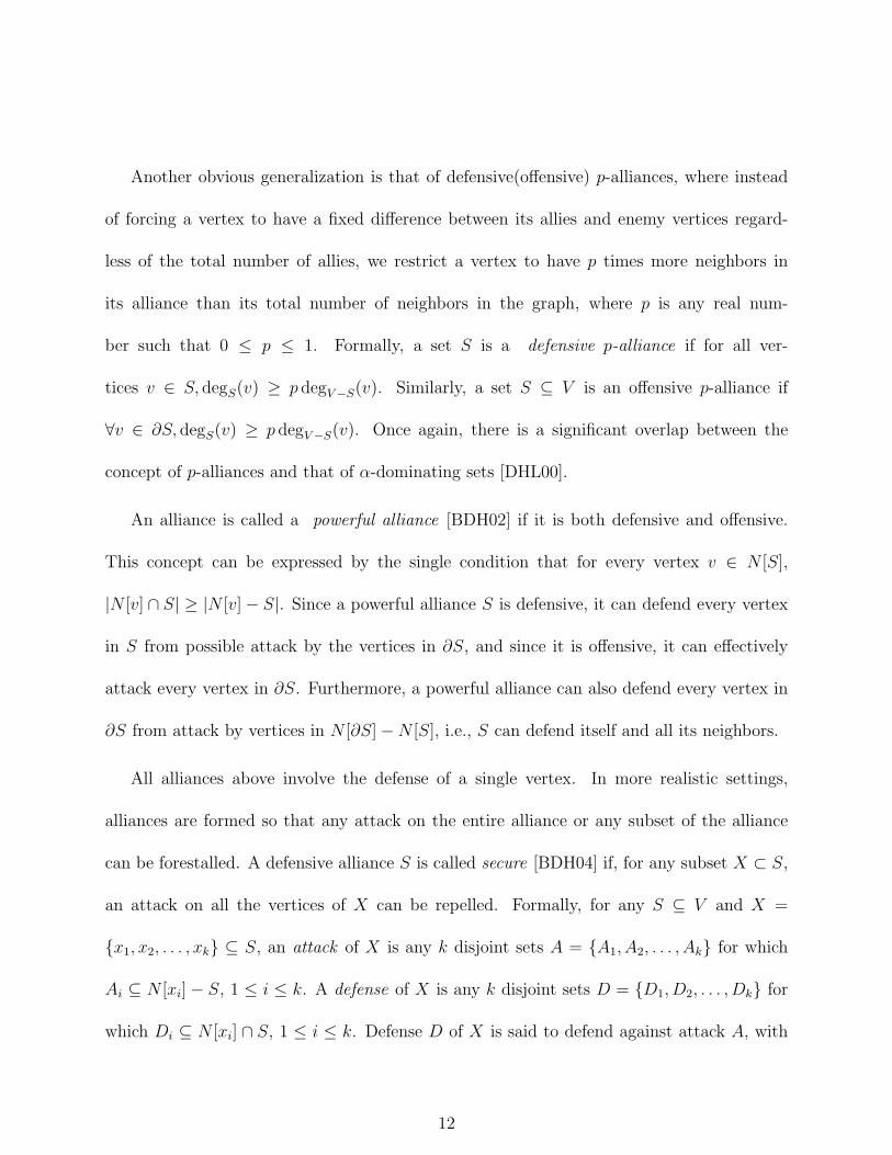
Another obvious generalization is that of defensive(offensive) p-alliances, where instead

of forcing a vertex to have a fixed difference between its allies and enemy vertices regard-

less of the total number of allies, we restrict a vertex to have p times more neighbors in

its alliance than its total number of neighbors in the graph, where p is any real num-

ber such that 0 ≤ p ≤ 1. Formally, a set S is a defensive p-alliance if for all ver-

tices v ∈ S, degS(v) ≥ p degV −S(v). Similarly, a set S ⊆ V is an offensive p-alliance if

∀v ∈ ∂S, degS(v) ≥ p degV −S(v). Once again, there is a significant overlap between the

concept of p-alliances and that of α-dominating sets [DHL00].

An alliance is called a powerful alliance [BDH02] if it is both defensive and offensive.

This concept can be expressed by the single condition that for every vertex v ∈ N [S],

|N [v] ∩ S| ≥ |N [v] − S|. Since a powerful alliance S is defensive, it can defend every vertex

in S from possible attack by the vertices in ∂S, and since it is offensive, it can effectively

attack every vertex in ∂S. Furthermore, a powerful alliance can also defend every vertex in

∂S from attack by vertices in N [∂S] − N [S], i.e., S can defend itself and all its neighbors.

All alliances above involve the defense of a single vertex. In more realistic settings,

alliances are formed so that any attack on the entire alliance or any subset of the alliance

can be forestalled. A defensive alliance S is called secure [BDH04] if, for any subset X ⊂ S,

an attack on all the vertices of X can be repelled. Formally, for any S ⊆ V and X =

{x1, x2, . . . , xk} ⊆ S, an attack of X is any k disjoint sets A = {A1, A2, . . . , Ak} for which

Ai ⊆ N [xi] − S, 1 ≤ i ≤ k. A defense of X is any k disjoint sets D = {D1, D2, . . . , Dk} for

which Di ⊆ N [xi] ∩ S, 1 ≤ i ≤ k. Defense D of X is said to defend against attack A, with

12

respect to the set S, whenever |Di| ≥ |Ai| for 1 ≤ i ≤ k. Alternatively, X is defendable from

attack by A. The set X is S-secure if it is defendable from attack by A. When X = S and

S is S − secure, S is said to be secure.

An alliance (of any type) is called global [HHH02] if it affects every vertex in V −S, i.e.,

every vertex in V − S is adjacent to at least one member of the alliance S. In other words

an alliance S is global if it is also a dominating set.

Note that all these alliances can be easily generalized to edge weighted and/or vertex

weighted graphs. Let f : E → < and g : V → <. A set S ⊆ V is called weighted defensive

alliance, if for all v ∈ S,∑

u∈NS [v] f(u, v)g(u) ≥ ∑

u∈NV −S(v) f(u, v)g(u). Alliances defined

earlier can be generalized to weighted graphs in a similar fashion. For the un-weighted cases,

the functions f and g may both be assumed to be equal to 1.

2.3 Alliance Numbers

In this section, we will introduce some parameters associated with the different types of

alliances. In general we will refer to all types of alliances simply as alliances and the param-

eters are collectively called alliance numbers. An alliance (of some type) is called critical or

minimal if no proper subset of S is an alliance (of the same type). In the rest of this text we

will ignore the parenthesized phrases emphasizing that the alliances of same types are the

topic of concern and will assume that it will always be the case unless specified otherwise.

13

Note that the property of being an alliance is not necessarily hereditary, i.e., a set contained

in an alliance is not necessarily an alliance. We define an alliance S to be locally minimal

or locally critical, if for all v ∈ S, S − {v} is not an alliance. Generalizing, we define an

alliance S to be r−critical or r−minimal if for all T ⊂ S such that |T | = r, S − T is not an

alliance. An alliance is minimum if it is a minimal alliance of smallest cardinality.

Similarly, an alliance S is maximal if it is not a proper subset of any other alliance. It is

k−maximal if for all T ⊆ V − S, such that |T | = k, S ∪ T is not an alliance. An alliance is

maximum if it is a maximal alliance of maximum cardinality.

The cardinality of minimum alliance of a graph G is called the alliance number of G,

while the largest cardinality of a minimal alliance of a graph G is called the upper alliance

number of G. (Note that the terms alliance number and upper alliance number are used for

the cardinalities of minimum defensive alliance and largest minimal defensive alliance of a

graph in [HHK00]. In this text, we will use the terms defensive alliance number and upper

defensive alliance number for these parameters). This leads to two invariants for each type

of alliance defined in the previous section. Of particular interest are the following invariants:

a(G) = the defensive alliance number of graph G

A(G) = the upper defensive alliance number of graph G

a(G) = the strong defensive alliance number of graph G

A(G) = the upper strong defensive alliance number of graph G

14

ak(G) = the defensive k-alliance number of graph G

Ak(G) = the upper defensive k-alliance number of graph G

ak(G) = the strong defensive k-alliance number of graph G

Ak(G) = the upper strong k-defensive alliance number of graph G

ao(G) = the offensive alliance number of graph G

Ao(G) = the upper offensive alliance number of graph G

ao(G) = the strong offensive alliance number of graph G

Ao(G) = the upper strong offensive alliance number of graph G

γa(G) = the global defensive alliance number of graph G

γa(G) = the global strong defensive alliance number of graph G

ap(G) = the powerful alliance number of graph G

ap(G) = the strong powerful alliance number of graph G

as(G) = the secure alliance number of graph G

From the definitions, it is easy to see that the following relations hold for the above

parameters;

i. a−1(G) = a(G) ≤ a(G) = a0(G) ≤ A(G) = A0(G),

ii. a(G) ≤ A(G) = A0(G),

iii. a(G) ≤ ad(G),

iv. a(G) ≤ γa(G),

15

v. a(G) ≤ ad(G),

vi. a(G) ≤ γa(G),

vii. ao(G) ≤ ao(G) ≤ Ao(G),

viii. ao(G) ≤ Ao(G),

ix. ao(G) ≤ ad(G),

x. ao(G) ≤ ad(G).

2.4 Basic Properties and Known Bounds on Alliance Numbers

The following subsections summarizes several observations and properties of different types

of alliances and respective alliance numbers.

2.4.1 Defensive Alliance Numbers

It has been shown in [MGH02] that finding a(G) and a(G) for arbitrary graph G is NP-

Hard, even when restricted to bipartite or chordal graphs. The classes of graphs for which

the values of a(G) and a(G) belong to the set {1, 2, 3} are summarized below:

16

Observation 1 [HHK00]

i. a(G) = 1 if and only if there exists a vertex v ∈ V such that deg(v) ≤ 1.

ii. a(G) = 1 if and only if G has an isolated vertex.

iii. a(G) = 2 if and only if δ(G) ≥ 2 and G has two adjacent vertices of degree at most

three.

iv. a(G) = 2 if and only if δ(G) ≥ 1 and G has two adjacent vertices of degree at most

two.

v. a(G) = 3 if and only if a(G) 6= 1, a(G) 6= 2, and G has an induced subgraph isomorphic

to either (a) P3, with vertices, in order, u, v, and w, where deg(u) and deg(w) are at

most three, and deg(v) is at most five, or (b) K3, each vertex of which has degree at

most five.

vi. a(G) = 3 if and only if a(G) 6= 1, a(G) 6= 2, and G has an induced subgraph isomorphic

to either (a) P3, with vertices, in order, u, v, and w, where deg(u) and deg(w) are at

most two, and deg(v) is at most four, or (b) K3, each vertex of which has degree at

most four.

The values of defensive alliance numbers for some special classes of graphs are also known

and are as follows:

Theorem 2 [HHK00] For the m × n grid graph Gm,n,

i. a(Gm,n) = 1 if and only if min{m,n} = 1.

17

ii. a(Gm,n) = 2 if and only if min{m,n} ≥ 2.

iii. a(Gm,n) = 2 if and only if min{m,n} < 3.

iv. a(Gm,n) = 3 if and only if min{m,n} = 3.

v. a(Gm,n) = 4 if and only if min{m,n} ≥ 4.

Theorem 3 [HHK00] For any graph G = (V,E),

i. if G is 1-regular, then a(G) = 1 and a(G) = 2.

ii. if G is 2-regular, then a(G) = 2 and a(G) = 2.

iii. if G is 3-regular, then a(G) = 2 and a(G) = girth(G).

iv. if G is 4-regular, then a(G) = a(G) = girth(G).

v. if G is 5-regular, then a(G) = girth(G).

For all the above classes of graphs, the values of defensive alliance numbers are constant,

however, for wheels, complete graphs, and complete bipartite graphs, these values can be

arbitrarily large. For wheels Wn of order n, a(Wn) =⌈

n2

⌉

. For the complete graph Kn,

a(Kn) =⌈

n2

⌉

and a(Kn) =⌊

n2

⌋

+ 1. Frick et al [FLH] showed that the complete graphs

achieve the upper bound for defensive alliance number a(G).

Theorem 4 [FLH] For any graph G of order n,

a(G) ≤⌈n

2

⌉

.

18

We now show that the even complete graphs achieve the upper bound for strong defensive

alliance number a(G), i.e., a minimum strong defensive alliance of graph G has at most

⌊

n2

⌋

+ 1 vertices.

Theorem 5 For any graph G, of order n, a(G) ≤⌊

n2

⌋

+ 1.

Proof. Let A be a minimum defensive 0-alliance of a graph G and B = V (G)−A. Assume

to the contrary that |A| >⌊

n2

⌋

+ 1. If ∃T ⊆ B and v ∈ A, such that Tor T ∪ {v} is a

defensive 0-alliance then |T |+ 1 ≤⌈

n2

⌉

− 1 < |A|, a contradiction. Thus, there is a partition

〈V1, V2〉 of V (G) such that ∀P ⊆ V1, P is not a defensive 0-alliance. Similarly, ∀Q ⊆ V2,

Q is not a defensive 0-alliance. Consider such a partition with the property that the size of

edge-cutset S separating V1 and V2 is minimum among all such partitions. Assume without

loss of generality that |V1| ≥⌈

n2

⌉

. Since V1 is not a defensive 0-alliance, ∃v ∈ V1 such that

degV1(v) < degV2

(v). Consider the partition 〈V1 − {v} , V2 ∪ {v}〉. Let S ′ be the edge-cutset

separating V1 −{v} and V2 ∪{v} such that |S ′| = |S|−degV2(v)+degV1

(v) < |S|. Hence, at

least one of the sets, V1 −{v} or V2 ∪{v}, must be a defensive 0-alliance or contain a subset

that is a defensive 0-alliance. Since V1 − {v} is not a defensive 0-alliance, V2 ∪ {v} must be

a defensive 0-alliance or contain a defensive 0-alliance, but then |V2 ∪ {v}| ≤⌊

n2

⌋

+ 1 < |A|,

a contradiction. ¤

19

2.4.2 Global Defensive Alliance Numbers

We now present some properties of global defensive alliance numbers γa(G) and γa(G). We

begin by giving values for specific graph families.

Proposition 6 [HHH02] For the complete graph Kn,

(i) γa(Kn) =⌊

n+12

⌋

, and

(ii) γa(Kn) =⌈

n+12

⌉

.

Proposition 7 [HHH02] For the complete bipartite graph Kr,s,

(i) γa(K1,s) =⌊

s2

⌋

+ 1,

(ii) γa(Kr,s) =⌊

r2

⌋

+⌊

s2

⌋

if r, s ≥ 2, and

(iii) γa(Kr,s) =⌈

r2

⌉

+⌈

s2

⌉

.

By definition, for every global defensive alliance S, ∂S = V −S, i.e., every global defensive

alliance set is a dominating set. Hence, γa(G) ≥ γ(G), where γ(G) is the domination number

of graph G.

A set D of vertices of G is defined to be a total dominating set if N(D) = V . In other

words, a total dominating set is a dominating set D with an added condition that every

vertex in D must also be adjacent to some other vertex of D. The total domination number

γt(G) of a graph G is the smallest cardinality of a total dominating set. It is easy to see

that for any graph G, γa(G) ≥ γt(G). In addition, the following lower bounds are known for

global defensive alliance numbers.

20

Theorem 8 [HHH02] If G is a graph of order n, then

γa(G) ≥(√

4n + 1 − 1)

/2,

γa(G) ≥ √n.

Both of the above bounds are tight and are achieved by the graphs Kk◦Kk and Kk◦Kk−1

respectively, where, for graphs G and H, the corona G ◦H is the graph formed from G and

|V (G)| copies of H, where the ith vertex of G is adjacent to every vertex in the ith copy of

H.

Theorem 9 [HHH02] If G is a graph of order n and maximum degree ∆, then

γa(G) ≥ 2n∆+3

,

γa(G) ≥ 2n∆+2

.

Cami et al [CBD04] have shown that the problem of computing γ(G) is NP-Hard. A

similar construction can be used to show a more general problem of minimum defensive

k-alliance is NP-Hard for any fixed k.

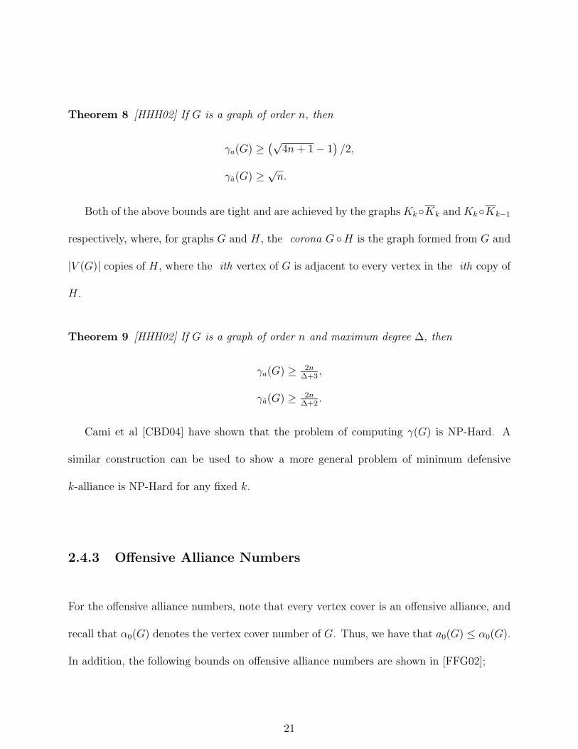
2.4.3 Offensive Alliance Numbers

For the offensive alliance numbers, note that every vertex cover is an offensive alliance, and

recall that α0(G) denotes the vertex cover number of G. Thus, we have that a0(G) ≤ α0(G).

In addition, the following bounds on offensive alliance numbers are shown in [FFG02];

21

Theorem 10 For all graphs G of order n ≥ 2, ao(G) ≤ 2n3.

Theorem 11 For all graphs G of order n ≥ 3, ao(G) ≤ 5n/6. Moreover, if G has minimum

degree at least 2, then ao(G) ≤ 3n/4.

Theorem 12 For graph G with order n and minimum degree δ, ao(G) ≤ ao(G) ≤ n (1/2 + o(δ)).

A tight upper bound or the extremal graphs for the strong offensive alliance numbers are

yet unknown.

As is the case with other alliance parameters, computing ao(G) and ao(G) is also an NP-

Hard problem, even for cubic graphs [FFG02]. Similarly, the problem of computing global

offensive alliance number is also NP-Hard.

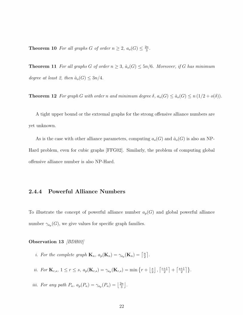
2.4.4 Powerful Alliance Numbers

To illustrate the concept of powerful alliance number ap(G) and global powerful alliance

number γap(G), we give values for specific graph families.

Observation 13 [BDH02]

i. For the complete graph Kn, ap(Kn) = γap(Kn) =

⌈

n2

⌉

.

ii. For Kr,s, 1 ≤ r ≤ s, ap(Kr,s) = γap(Kr,s) = min

{

r +⌊

s2

⌋

,⌈

r+12

⌉

+⌈

s+12

⌉}

.

iii. For any path Pn, ap(Pn) = γap(Pn) =

⌊

2n3

⌋

.

22

iv. For any cycle Cn, ap(Cn) = γap(Cn) =

⌈

2n3

⌉

.

We define a problem PA(POWERFUL ALLIANCE) to be the problem of deciding

whether a given graph has a powerful alliance of size less than or equal to a given bound

K. Similarly the problem GPA(GLOBAL POWERFUL ALLIANCE) is defined to be the

problem of deciding whether a given graph has a global powerful alliance of size less than or

equal to a given bound K. It is shown in [CBD04] that GPA is NP-Complete. We now show

that the problem PA is also NP-Complete by showing that an NP-Complete variant of GPA

is polynomially reducible to PA. The problems we are interested in are formally defined as

follows:

GLOBAL POWERFUL ALLIANCE (GPA)

Input: A Graph G(V,E) and a positive integer K ≤ |V |.

Question: Is there a global powerful alliance in G of size K or less?

AT MOST HALF GLOBAL POWERFUL ALLIANCE (AHGPA)

Input: A Graph G(V,E).

Question: Is there a global powerful alliance in G of size |V |2

or less?

POWERFUL ALLIANCE (PA)

Input: A Graph G(V,E) and a positive integer K ≤ |V |.

Question: Is there a powerful alliance in G of size K or less?

Theorem 14 AT MOST HALF GLOBAL POWERFUL ALLIANCE (AHGPA) is NP-

Complete.

23

Proof. It is easy to see that AHGPA is in NP. Given an instance of GPA, i.e., a graph

G = (V,E) and a positive integer K ≤ |V |, where V = {v1, v2, . . . , vn}, we transform the

instance of GPA into an instance of AHGPA by constructing a graph G′ = (V ′, E ′) as follows:

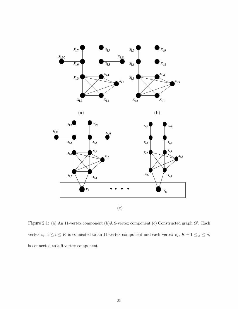
Let V ′ = V ∪ A1 ∪ A2 ∪ . . . ∪ An, where for 1 ≤ i ≤ K, Ai = {xi,j, 1 ≤ j ≤ 11} is a

component of 11 vertices, and for K + 1 ≤ i ≤ n, Ai = {xi,j, 1 ≤ j ≤ 9} is a component of

9 vertices. Both types of components are shown in Figure 2.1. Thus |V ′| = 10n + 2K. The

vertices xi,1 and xi,2 of each component Ai are adjacent to the vertex vi ∈ V . We define Ei

to be the set of edges incident to the vertices in Ai, 1 ≤ i ≤ n. As shown in the figure, for

i ≤ K,

Ei = {xi,jxi,k|1 ≤ j < k ≤ 5}∪{xi,3xi,6, xi,6xi,7, xi,4xi,8, xi,8xi,9, xi,6xi,10, xi,8xi,11, vixi,1, vixi,2},

and for i > K, Ei = {xi,jxi,k|1 ≤ j < k ≤ 5} ∪ {xi,3xi,6, xi,6xi,7, xi,4xi,8, xi,8xi,9, vixi,1, vixi,2}.

Define the edge set E ′ of the constructed graph G′ as

E ′ = E ∪(

⋃

1≤i≤n

Ei

)

.

We now claim that the constructed graph G′ has a global powerful alliance of size less

than or equal to |V ′|2

if and only if the given graph G has a global powerful alliance of size

less than or equal to K. The proof of the claim is as follows:

=⇒ Suppose that the given graph G has a global powerful alliance S of size less than or

equal to K. Consider a set T = S ∪(⋃

1≤i≤n{xi,2, xi,3, xi,4, xi,6, xi,8})

. Since S is a global

powerful alliance in G, for each vi ∈ V , |NS[vi]| ≥ |NV −S[vi]|. By construction, for each

vi ∈ V , NT−V [vi] = {xi,2} and NV ′−V −T [vi] = {xi,1}. Hence, |NT [vi]| = |NS[vi]| + 1 ≥

24

xi,1

xi,5

xi,4xi,3

xi,2

xi,6 xi,8

xi,7 xi,9

xi,10 xi,11

xi,1

xi,5

xi,4xi,3

xi,2

xi,6 xi,8

xi,7 xi,9

xi,10 xi,11

xi,1

xi,5

xi,4xi,3

xi,2

xi,6 xi,8

xi,7 xi,9

xi,1

xi,5

xi,4xi,3

xi,2

xi,6 xi,8

xi,7 xi,9

(a) (b)

x1,1

x1,5

x1,4x1,3

x1,2

x1,6 x1,8

x1,7 x1,9

x1,10 x1,11

xn,1

xn,5

xn,4xn,3

xn,2

xn,6 xn,8

xn,7 xn,9

v1 v

n

x1,1

x1,5

x1,4x1,3

x1,2

x1,6 x1,8

x1,7 x1,9

x1,10 x1,11

xn,1

xn,5

xn,4xn,3

xn,2

xn,6 xn,8

xn,7 xn,9

v1 v

n

(c)

Figure 2.1: (a) An 11-vertex component (b)A 9-vertex component.(c) Constructed graph G′. Each

vertex vi, 1 ≤ i ≤ K is connected to an 11-vertex component and each vertex vj , K + 1 ≤ j ≤ n,

is connected to a 9-vertex component.

25

|NV −S[vi]| + 1 = |NV ′−T [vi]|. Furthermore, for all x ∈ ⋃

1≤i≤n Ai, |NT [x]| ≥ |NV ′−T [x]|.

Thus, T is a powerful alliance and |T | ≤ 5n + K = |V ′|2

.

⇐= Let S ′ be a global powerful alliance of the constructed graph G′, such that |S ′| ≤ |V ′|2

=

5n + K. From the construction of graph G′, it is easy to see that any global powerful

alliance must contain at least five vertices from each Ai, 1 ≤ i ≤ n. Thus |S ′ ∩ V | ≤ K.

Let S = S ′ ∩ V and WS′ = {vi|NS[vi] < NV −S[vi]}. Let S ′ be a minimum global powerful

alliance in graph G′, such that |WS′| is minimum among all such alliances.

Suppose now that WS′ 6= ∅ and let vi ∈ WS′ . Since S ′ is a global powerful alliance, we

must have {xi,1, xi,2} ⊂ S ′ and 2 ≤ |NS′ [vi]| = |NV ′−S′ [vi]| = |NV −S′ [vi]|. Also, by the design

of component Ai and the definition of global powerful alliance, |S ′∩Ai| ≥ 6. Arbitrarily pick

a vertex vj ∈ NV −S′(vi) and consider the set T ′ = (S ′ − Ai)∪ {xi,2, xi,3, xi,4, xi,6, xi,8} ∪ {vj}.

Note that all the vertices in V ′ − Ai have equal or more neighbors (including themselves)

in T ′ than they had in S ′. Also, for all vertices a ∈ Ai, NT ′ [a] ≥ NV ′−T ′ [a]. Hence, T ′ is

a minimum global powerful alliance in graph G′ and WT ′ = WS′ − {vi}, which is contrary

to WS′ being a minimum such set. Hence WS′ = ∅, i.e., for all i, NS[vi] ≥ NV −S[vi], which

implies that S is a global powerful alliance in graph G. ¤

Now that we have shown that AHGPA is NP-Complete, we prove that POWERFUL

ALLIANCE (PA) is also NP-Complete.

Theorem 15 POWERFUL ALLIANCE (PA) is NP-Complete.

26

Proof. It is easy to see that PA is in NP. Given an instance of AHGPA, i.e., a graph

G = (V,E), where V = {v1, v2, . . . , vn}, we transform the instance of AHGPA into an

instance of PA by setting K ′ =⌊

3n2

⌋

+ 2 and constructing a graph G′ = (V ′, E ′) as follows:

Figure 2.2: (a) Construction of an instance of PA from an instance of AHGPA.

The vertex set V ′ of the graph G′ is defined as V ′ = V ∪W ∪X∪Y ∪{z1, z2}, where W =

{w1, w2, . . . , wn}, X = {x1, x2, . . . , xn}, Y = {y1, y2, . . . , yn}. W , X and Y are independent

sets, such that for all wi ∈ W , N(wi) = {xi, z2}, for all xi ∈ X, N(xi) = {vi, wi, yi, z1, z2},

and for all yi ∈ Y , N(yi) = {vi, xi, z1}. Also, N(z1) = X ∪ Y and N(z2) = X ∪ W . (See

Figure 2.2). Formally, the edge set E ′ of the constructed graph G′, is defined as

E ′ = E ∪(

⋃

1≤i≤n

{wixi, wiz2, xivi, xiyi, xiz1, xiz2, yivi, yiz1})

27

The order of the constructed graph, |V ′| = 4n+2 and the size of the graph, |E ′| = |E|+8n,

which are polynomially related to the size of the AHGPA problem. We now claim that the

constructed graph G′ has a powerful alliance of size less than or equal to K ′ =⌊

3n2

⌋

+ 2 if

and only if the given graph G has a global powerful alliance of size less than or equal to n2.

=⇒ Suppose that the given graph G has a global powerful alliance S of size less than or

equal to n2. Let S = {v1, v2, . . . , vr}, r ≤ n

2. Consider a set T = S ∪ X ∪ {z1, z2}. Since S

is a global powerful alliance in G, for each vi ∈ V , |NS[vi]| ≥ |NV −S[vi]|. By construction,

for each vi ∈ V , |NT−V [vi]| = 1 and |NV ′−V −T [vi]| = 1. Hence, |NT [vi]| = |NS[vi]| + 1 ≥

|NV −S[vi]| + 1 = |NV ′−T [vi]|. Similarly, for all vertices xi ∈ X, |NT [xi]| ≥ 3 ≥ |NV ′−T [xi]|.

For all yi ∈ Y , |NT [yi]| ≥ 2 ≥ |NV ′−T [yi]|. For all wi ∈ W , |NT [wi]| = 2 > |NV ′−T [wi]| = 1.

Finally, |NT [z1]| = n + 1 > |NV ′−T [z1]| = n and |NT [z2]| = n + 1 > |NV ′−T [z2]| = n. Since

for all vertices v ∈ N [T ], |NT [v]| ≥ |NV ′−T [v], T is a powerful alliance in graph G′ and

|T | = r + n + 2 ≤⌊

3n2

⌋

+ 2 = K ′.

⇐= Suppose that the constructed graph G′ has a powerful alliance of size less than or equal

to K ′ =⌊

3n2

⌋

+ 2. We now present a sequence of results, which culminate with the proof

that the graph G has a global powerful alliance of size less than or equal to n2.

Lemma 16 If S ′ is a powerful alliance in graph G′ such that |S ′| ≤⌊

3n2

⌋

+2, then {z1, z2} ⊆

S ′.

Proof. Assume to the contrary, and first let S ′ − V = ∅ and let S ′ = {v1, v2, . . . , vr}. Then

for all xi, 1 ≤ i ≤ r, |NS′ [xi]| = 1 < |NV ′−S′ [xi]| = 5, which is contrary to S ′ being a powerful

set. Thus, S ′ − V 6= ∅. Since for all u ∈ V ′ − V , {z1, z2} ∩ N [u] 6= ∅, {z1, z2} ∩ N [S ′] 6= ∅.

28

We now consider two exhaustive cases:

Case 1: S ′ ∩ {z1, z2} = ∅. Consider zi ∈ {z1, z2} ∩ N [S ′]. By the definition of powerful

alliance, |NS′(zi)| ≥ |NV ′−S′ [zi]|. From the construction, |N [zi]| = 2n + 1, therefore we have,

|NS′(zi)| ≥ n + 1. Let X ′ = {xi|{xi, yi} ∩ NS′(zi) 6= ∅}. Since N(zi) =⋃

1≤i≤n{xi, yi},

|X ′| ≥⌊

n2

⌋

+ 1. Also note that for all xi ∈ X ′, |N [xi]| = 6, hence, we must have |NS′ [xi]| =

|{vi, wi, xi, yi, z1, z2} ∩ S ′| ≥ 3, which implies that, for all xi ∈ X ′, |{vi, wi, xi, yi} ∩ S ′| ≥ 3.

Thus |S ′| ≥ 3|X ′| = 3⌊

n2

⌋

+ 3 > K ′, a contradiction.

Case 2: |S ′ ∩ {z1, z2}| = 1. Since for all xi ∈ X, {z1, z2} ⊂ N [xi], X ⊂ N [S ′]. Hence, we

must have |NS′ [xi]| ≥ 3. That is, for all xi ∈ X, |{vi, wi, xi, yi} ∩ S ′| ≥ 2, which implies that

|S ′| ≥ 2|X| + 1 = 2n + 1 > K ′, again a contradiction.

Since both cases lead to contradiction, we must assume that {z1, z2} ⊆ S ′. ¤

Corollary 17 If S ′ is a powerful alliance in graph G′ such that |S ′| ≤⌊

3n2

⌋

+ 2, then

|S ′ − V | ≥ n + 2.


3n2

⌋

+ 2, then

(V ′ − V ) ⊆ N [S ′].


3n2

⌋

+ 2, then for all i,

1 ≤ i ≤ n, S ′ ∩ {wi, xi} 6= ∅.

Proof. From Corollary 18, W ⊂ N [S ′]. Since for all wi ∈ W , N [wi] = {wi, xi, z2}, by the

definition of power alliance, |NS′ [wi]| ≥ 2, i.e., |S ′ ∩ {wi, xi}| ≥ 1. ¤

29


3n2

⌋

+ 2, then for all i,

1 ≤ i ≤ n, S ′ ∩ {vi, xi, yi} 6= ∅.

Proof. From Corollary 18, Y ⊂ N [S ′]. Since for all yi ∈ Y , N [yi] = {vi, xi, yi, z1}, by the

definition of power alliance, |NS′ [yi]| ≥ 2, i.e., |S ′ ∩ {vi, xi, yi}| ≥ 1. ¤


3n2

⌋

+ 2, then

V ⊂ N [S ′].


3n2

⌋

+ 2, then S ′ is

a global powerful alliance.


3n2

⌋

+ 2, then S ′ ∩ V

is a global powerful alliance in graph G.

Proof. Let S ′ be a powerful alliance of the constructed graph G′, such that |S ′| ≤⌊

3n2

⌋

+ 2.

Let S = S ′ ∩ V and US′ = {vi|NS[vi] < NV −S[vi]}. Let S ′ be a powerful alliance for which

|US′ | is minimum among all such powerful alliances in the graph G′ of size less than or equal

to⌊

3n2

⌋

+ 2. If US′ = ∅ then S ′ ∩ V is a global powerful alliance in graph G.

Suppose now that US′ 6= ∅. Let vi ∈ US′ . From Corollary 22, S ′ is a global powerful

alliance, hence, we must have {xi, yi} ⊂ S ′ and 2 ≤ |NS′ [vi]| = |NV ′−S′ [vi]| = |NV −S′ [vi]|.

Arbitrarily pick a vertex vj ∈ NV −S′(vi) and consider the set T ′ = (S ′ − {yi}) ∪ {vj}. Note

that for all u ∈ V ′ − {xi, yi, z1}, |NT ′ [u]| ≥ |NS′ [u]|. Also, |NT ′ [xi]| ≥ 4 > |NV ′−T ′ [xi]| and

|NT ′ [yi]| = 3 > |NV ′−T ′ [yi]|. Now there are two cases:

30

Case 1: |NT ′ [z1]| ≥ |NV ′−T ′ [z1]|. Then for all vertices u ∈ V ′, NT ′ [u] ≥ NV ′−T ′ [u], i.e., T ′

is a powerful alliance. In addition, |T ′| = |S ′|, and |UT ′ | < |US′ |, a contradiction.

Case 2: |NT ′ [z1]| < |NV ′−T ′ [z1]|. From Lemma 17, we have, |NT ′ [z1]| = n. Since z1 ∈

T ′, by pigeonhole principle, there exists a set {xk, yk} such that {xk, yk} ∩ T ′ = ∅. From

Lemma 19, wk ∈ T ′. Let T = (T ′ − {wk}) ∪ {xk}. It is easy to see that for all the vertices

u ∈ V ′, NT [u] ≥ NV ′−T [u]. Hence T is a powerful alliance in graph G′ with |T | = |T ′| = |S ′|,

and |UT | < |US′ |, a contradiction.

Since both cases lead to contradiction, we must conclude that our initial assumption that

US′ 6= ∅ was incorrect. Thus, S ′ ∩ V is a global powerful alliance in graph G. ¤

It follows from Corollaries 17 and 22, and from Lemma 23 that if the constructed graph

G′ has a powerful alliance of size less than or equal to K ′ =⌊

3n2

⌋

+ 2, then the graph G has

a global powerful alliance of size less than or equal to n2. ¤

2.5 Open Problems

We conclude this chapter with a list of open problems relating to alliances and alliance

numbers.

• Determine the relationships between alliance numbers (defensive, offensive, global, etc.)

and other domination parameters.

31

• Find the real upper bound for the offensive alliance numbers and the extremal graphs.

• Characterize the graphs (or some family of graphs) for which γ(G) = γa(G).

• Characterize the graphs (or some family of graphs) for which γt(G) = γa(G).

• Characterize the graphs (or some family of graphs) for which ao(G) = ao(G).

• Characterize the graphs (or some family of graphs) for which ao(G) = αo(G).

• Determine the computational complexity of computing the parameters A(G), Ao(G),

ad(G), ad(G), γa(G), and γa(G).

• Study the alliance numbers for k−alliances and p-alliances.

• Study the global counterparts for alliances other than defensive alliances.

• Determine the exact values or good bounds for special families of graphs (e.g., trees,

grid graphs, planar, outer-planar graphs).

• Given a graph G and a vertex v ∈ V , define the alliance number (of some type) of

v, a(v) to be the smallest alliance (of that type) containing vertex v. What is the

complexity of finding a(v) (for each each type of alliance)?

• Given a graph G and a set S ∈ V , what is a(S), that is the smallest cardinality of an

alliance containing set S (for each type of alliance)?

• Given a graph G, define alliance packing numbers Pa(G) to equal the maximum num-

ber of pairwise-disjoint, alliances contained in G. Similarly, define alliance partitioning

32

numbers, ψa(G), to equal the maximum order of a partition Π = {V1, V2, . . . , Vk} of

V (G), such that each block of the partition Vi is an alliance. What is the complexity

of finding Pa(G) and ψa(G) for each type of alliance.

• Find exact efficient algorithms for computing the alliance numbers that are not NP-

Hard.

• Find the approximate algorithms for the alliance numbers that are NP-Hard.

• What is the minimum error that can be guaranteed to compute the alliance numbers

in polynomial time?

33

CHAPTER 3

PARTITIONING A GRAPH INTO DEFENSIVE

AND GLOBAL DEFENSIVE ALLIANCES

3.1 Introduction

In this chapter, we discuss the problem of partitioning a graph into defensive and strong

defensive alliances. The problem of partitioning a graph into strong defensive alliances was

first introduced by Gerber and Kobler [GK00] and was referred to as “Satisfactory Graph

Partitioning Problem (SGP)”.

Consider a graph G = (V,E) without loops or multiple edges. Recall from chapter 2 that

a vertex v in set A ⊆ V is said to be k-satisfied with respect to A if degA(v) ≥ degV −A(v)+k,

where degA(v) = |N(v) ∩ A| = |NA(v)| = deg(v) − degV −A(v). Also recall that a set A is

a defensive k- alliance if all vertices in A are k-satisfied with respect to A. Note that a

defensive (−1)-alliance is a “defensive alliance” (as defined in [HHK00]), and a defensive

0-alliance is a “strong defensive alliance” or “cohesive set” [SD02a]. A k-defensive alliance

34

A is called global if every vertex in V −A is adjacent to at least one member of the alliance

A.

A graph is said to be k-satisfiable if there exists a vertex partition into two or more

nonempty sets so that every vertex is k-satisfied with respect to the set in which it occurs, i.e.,

a partition into two or more k-defensive alliances (it is called k−unsatisfiable otherwise).

Such a partition is referred to as k-satisfactory partition .

Our problem, the k- Satisfactory Graph Partitioning problem (k-SGP), consists in deter-

mining if a graph is k-satisfiable or not, i.e., whether a given graph can be partitioned into

two k-defensive alliances. The problem can be easily generalized to other types of alliances.

Of particular interest are weighted defensive k−alliances and weighted defensive p-alliances.

A related problem has been considered in Artificial Intelligence to study a neural net-

work model of the human brain known as binary coherent system (BCS)[Hop82] or stable

configuration problem[SY91]. The problem can be formally stated as follows: Given an edge

weighted directed graph G = (V,E) and a threshold value tv for each vertex v ∈ V . Find

a partition 〈V−1, V+1〉 of V such that for every vertex v, the energy E(v) is non-negative,

where,

E(v) = sv

tv +∑

e=(u,v)∈E

wesu

sv = 1, if v ∈ V+1 and sv = −1, otherwise.

35

Note that BCS problem allows a set in a partition to be empty, while SGP does not. The

BCS problem has a polynomial time sequential algorithm if all of the weights and thresholds

are input in unary [Lub86].

The Different Than Majority Labelling (DTML) problem [Lub86] is a special case of the

BCS problem. Here the threshold value tv is 0 for every vertex v, and all edge weights are -1.

The DTML problem may also be viewed as a similar but complementary graph partitioning

problem of 0-SGP known as Unfriendly Graph Partitioning Problem (UGP) [BK], where a

partition is said to be unfriendly if each vertex has as many or more neighbors outside the set

in which it occurs than inside it. While there exists an unfriendly graph partition for every

graph1, this is not the case for satisfactory partitions of vertices. For example, complete

graphs Kn and complete bipartite graphs Kp,q (when p or q is odd) are not 0-satisfiable.

Similarly, odd complete graphs are not (−1)-satisfiable. There exists a polynomial time

algorithm for finding an unfriendly partition for graphs. On the other hand, the problem

k-SGP, k ≥ 0, was also shown to be NP-Hard for unweighted graphs in [BTV03a, BTV03b].

For k < −1, every graph has a k-satisfactory partition[Sti96], and such a partition can be

found in polynomial time[BTV03b].

Another complementary problem of SGP is that of partitioning the vertex set into two

or more sets such that none of these sets contain any k-alliance, i.e., a partition into k-

alliance-free sets. The existence of such a partition is again not guaranteed, for example

1All finite graphs have unfriendly bipartitions, but there exist infinite graph with no unfriendly bipartition[SM90]. However, all graphs have an unfriendly 3-partition

36

complete graphs of odd order and odd cycles do not have a partition into 0−alliance free

sets. However, we have characterized the graphs that have such a partition[SD04].

In this chapter, we present results on the solution and the complexity of the following

problems.

PARTITION INTO DEFENSIVE ALLIANCES ((−1)-SGP)


Question: Is there a partition 〈V1, V2〉 of V , such that both V1 and V2 are defensive

alliances ((−1)-defensive alliances)

PARTITION INTO STRONG DEFENSIVE ALLIANCES (0-SGP)


Question: Is there a partition 〈V1, V2〉 of V , such that both V1 and V2 are strong defensive

alliances (0-defensive alliances)

PARTITION INTO GLOBAL DEFENSIVE ALLIANCES


Question: Is there a partition 〈V1, V2〉 of V , such that both V1 and V2 are global defensive

alliances (global (−1)-defensive alliances)

PARTITION INTO GLOBAL STRONG DEFENSIVE ALLIANCES


Question: Is there a partition 〈V1, V2〉 of V , such that both V1 and V2 are global strong

defensive alliances (global 0-defensive alliances)

37

The organization of this chapter is as follows. In Section 2, we present some basic

observations. Section 3 discusses the relationship between satisfiability and connectivity

of graphs. Section 4 presents results regarding categorization of satisfiable graph by their

subgraphs. Section 5 treats special cases, for example, Eulerian graphs, regular graphs and

line graphs. Section 6 concludes the chapter.

Since, disconnected graphs are trivially satisfiable, we will only consider connected graphs.

3.2 Basic Properties

Since every defensive k-alliance is also a defensive l-alliance, for all l < k and since every

global defensive k-alliance is also a defensive k-alliance, our first observation is immediate.

Observation 24 For any graph G

(i) If G has a k-satisfactory partition then G has an l-satisfactory partition, for all l < k.

(ii) If G has a partition into global defensive k-alliances then G has a k-satisfactory parti-

tion.

Also, since for an Eulerian graph a (2r − 1)-defensive alliance is also a 2r-defensive

alliance, we have,

Observation 25 For an Eulerian graph G and r ≤ δ(G)2

, a partition into (global) (2r − 1)-

defensive alliances is also a partition into (global) 2r-defensive alliances.

38

Since V (G) is itself a defensive k-alliance, k ≤ δ(G), we define a defensive k-alliance

X ⊂ V to be locally maximal if ∀v /∈ X, X ∪ {v} is not a defensive k-alliance. If X is a

locally maximal defensive k-alliance of graph G then V (G)−X is a defensive (1−k)-alliance.

Proposition 26 For k ≤ 0, a graph G is k-satisfiable if it has a locally maximal defensive

k-alliance.

The converse of the above proposition is not true, for example, Cn,∀n > 3 is 0-satisfiable

but has no locally maximal defensive 0-alliance.

Similarly, a locally minimal defensive k-alliance is a defensive k-alliance X, such that

∀v ∈ X, X − {v} is not a defensive k-alliance. Every minimal defensive k-alliance is also

a locally minimal defensive k-alliance but a locally minimal defensive k-alliance need not

be a minimal defensive k-alliance. A minimum defensive k-alliance is a minimal defensive

k-alliance of smallest order. If a graph G is k-satisfiable, then, by definition, it has at least

two disjoint minimal defensive k-alliances (the converse of this is also true and is Lemma 27).

Lemma 27 [Sti96] For k ≤ 0, a graph G is k-satisfiable if and only if it has two disjoint

k-alliances.

Hence, if every minimal defensive k-alliance of a graph G has at least⌊

n2

⌋

+ 1 vertices

then G is k-unsatisfiable. From Theorems 4 and 5, we know that a minimum defensive

(-1)-alliance of a graph has at most⌈

n2

⌉

vertices, whereas a minimum defensive (0)-alliance

has no more than⌊

n2

⌋

+ 1 vertices.

39

Next we present the satisfiability of some common graph families.

Observation 28 The following graphs have partition into strong defensive alliances ( i.e.,

they are 0-satisfiable):

(i) Complete graphs of even order minus a 1-factor.

(ii) Complete bipartite graphs Kp,q if both p and q are even.

(iii) Grid graphs.

(iv) Cycles of order greater than 3.

(v) Separable graphs and graphs that have a bridge, which is not a pendant edge, for ex-

ample, trees with diameter greater than 2.

The first two of the above graphs also have a partition into global strong defensive

alliances. From Observation 24, all the above graphs also have a partition into defensive

alliances. Examples of graphs that have a partition into defensive alliances are presented in

the next observation.

Observation 29 The following graphs have partition into defensive alliances ( i.e., they are

(−1)-satisfiable):

(i) Complete graphs of even order.

(ii) Complete bipartite graphs.

40

(iii) Graphs that have one or more pendant vertices.

The following result was shown in [GK01]:

Theorem 30 [GK01] Every graph (that is not K1,n) of girth at least 5 is 0-satisfiable.

3.3 Satisfiability and Connectivity

In this section, we discuss the relation between the connectivity and satisfiability of a

graph. We know that complete graphs are 0-unsatisfiable and that trees, except stars, are

0-satisfiable. We first ask if there is a bound for which graphs with minimum degree greater

than this bound are k-unsatisfiable, for k ∈ {−1, 0}. We prove next that no such bound

exists.

Theorem 31 There is no r ∈ [0, 1) such that δ (G) ≥ rn ⇒ G is 0-unsatisfiable.

Proof. Note that ∀p ≥ 1,K2p minus 1-factor is 0-satisfiable, where V1 and V2 form a 0-

satisfactory partition such that G [V1] ∼= G [V2] ∼= Kp. Assume to the contrary that such an

r exists. Consider p ≥ 11−r

, and let G ∼= K2p minus a 1-factor. Then δ (G) = 2p− 2. Since G

is 0-satisfiable, therefore by assumption, 2p − 2 < r (2p) ⇒ p < 11−r

, hence a contradiction.

¤

Similarly it can be proved that there is no r ∈ [0, 1) such that density (G) ≥ r ⇒ G is

0-unsatisfiable, where density (G) = |E|n(n−1)/2

.

41

We define a Critical Cutset S = 〈V1, V2〉 of a connected graph G to be a minimal cutset,

such that |Vi| > 1, i ∈ { 1, 2} and moving any vertex from one set to the other does not

decrease the size of the resulting cutset.

Theorem 32 G is 0-satisfiable if and only if it has a critical cutset.

Proof. Suppose G has a critical cutset S = 〈V1, V2〉 and there exists a vertex v which is

not 0-satisfied. Assume without loss of generality that v ∈ V1. Then degV1(v) < degV2

(v)

and we may form a new partition S ′ = 〈V1 − {v} , V2 ∪ {v}〉 where |V1 − {v}| ≥ 1. Now,

|S ′| = |S| − degV2(v) + degV1

(v). Since degV1(v) < degV2

(v), we must have that |S ′| < |S|,

contradicting the assumption that S is a critical cutset of G.

For the converse, consider a 0-satisfiable graph G such that the cutset S = 〈V1, V2〉 forms

a 0-satisfactory partition. Suppose that S is not a critical cutset, that is, there exists a

vertex v, such that moving v from one set of the partition to another would decrease the size

of cutset. Assume without loss of generality that v ∈ V1. Then S ′ = 〈V1 − {v} , V2 ∪ {v}〉

and |S ′| < |S|. But |S ′| = |S| − degV2(v) + degV1

(v) which means that degV1(v) < degV2

(v)

and contradicts the assumption that S = 〈V1, V2〉 is a 0-satisfactory partition. ¤

Recall that edge connectivity κ1 (G) of a graph G is the minimum number of edges whose

removal from G results in a disconnected graph. The following result, also proven in [GK00],

is a direct consequence of Theorem 32.

Corollary 33 A connected graph G is 0-satisfiable if κ1 (G) < δ (G).

42

The next theorem provides the relation between 0-satisfiability and vertex connectivity

κ (G);

Theorem 34 For k ≤ 0, a graph G is k-satisfiable if κ (G) ≤⌊

δ(G)−k

2

⌋

.

Proof. Suppose for a graph G, that κ (G) ≤⌊

δ(G)−k

2

⌋

and G is k-unsatisfiable. From

Corollary 33, we may assume G is connected and that V ′ is a set of disconnecting vertices

of G such that 1 ≤ |V ′| ≤⌊

δ(G)−k

2

⌋

. Let A be the set of vertices of one of the components

of G − V ′ and let B = V − V ′ − A. The edge cutset S = 〈B,A ∪ V ′〉 partitions V into two

subsets. Since ∀v ∈ B, N (v) ∩ A = ∅, N (v) − B ⊆ V ′, and thus degV −B (v) ≤⌊

δ(G)−k

2

⌋

≤

degB (v)− k. Hence, every vertex of B is k-satisfied. The only vertices in G, which may not

be k-satisfied with respect to the partition 〈B,A ∪ V ′〉, are those in V ′. Now perform the

following procedure on the partition.

While ∃v ∈ V ′ such that degV −B (v) < degB (v) + k

Begin

Set B ← B ∪ {v} , V ′ ← V ′ − {v}

End

This procedure will certainly terminate, as there is only a finite number of elements in

V ′ and vertices are only moved from set V ′ to set B. Since every vertex of B was initially

k-satisfied, no vertices are removed from B. Therefore every vertex of B is still k-satisfied.

Also, all vertices of V ′ are now k-satisfied. Since at most⌊

δ(G)−k

2

⌋

vertices were moved from

43

set V ′ to set B, vertices of A are each adjacent to at most⌊

δ(G)−k

2

⌋

vertices in B, and are

k-satisfied. Thus, G is k-satisfiable. ¤

3.4 Subgraph Characterizations

In this section we show that there is no forbidden subgraph characterization of minimal

defensive k-alliances. We also show that the same holds for satisfiable and unsatisfiable

graphs.

To show the nonexistence of a forbidden subgraph characterization for satisfiable graphs,

we first prove that for k ≤ 0, there is no such characterization for minimal defensive k-

alliances.

Lemma 35 For k ≤ δ(G), there is no forbidden subgraph characterization for subgraphs

induced by minimal defensive k-alliances.

Proof. Suppose to the contrary that G = (V,E) is a forbidden subgraph for graphs induced

by minimal defensive k-alliances. Since minimal alliances are connected, we may assume that

G is connected. Let V = {v1, v2, . . . , vn}, and construct a graph G′ = (V ′, E ′) as follows:

V ′ = V ∪X1∪X2∪ . . .∪Xn, where Xi ={

x(i)1 , x

(i)2 , . . . , x

(i)deg(vi)−k

}

is a set of independent

vertices; and E ′ = E ∪ Y1 ∪ Y2 ∪ . . . ∪ Yn, where Yi ={

vix(i)1 , vix

(i)2 , . . . , vix

(i)deg(vi)−k

}

. Hence,

by construction, ∀v ∈ V, degV (v) = degV ′−V (v) + k. Since G is connected, V is a minimal

k-alliance of graph G′, contradicting our initial assumption. ¤

44

Theorem 36 For k ≤ δ(G), there is no forbidden subgraph characterization of k-satisfiable

graphs.

Proof. Suppose to the contrary that G = (V,E) is a forbidden subgraph for graphs induced

by k-satisfiable graphs. Hence, G cannot be induced by any subset of a k-satisfiable graph.

Construct a graph G′ = (V ′, E ′) as in the proof of Lemma 35, such that V is a minimal k-

alliance of G′. Add edges between all the vertices in V ′ − V . From construction, |V ′ − V | =

2|E| − kn. Hence V ′ − V forms a clique of 2|E| − kn vertices and hence is a defensive

k-alliance. Thus, V and V ′ − V is a k-satisfactory partition of graph G′, a contradiction. ¤

Note that the graph constructed in the above proof has a partition into global defensive

k-alliances. Thus we have:

Corollary 37 For k ≤ δ(G), there is no forbidden subgraph characterization of the graphs

having a partition into global defensive k-alliances.

The join of simple graphs G1 and G2, written G1 ∨ G2, is the graph obtained by adding

the edges {xy : x ∈ V (G1) , y ∈ V (G2)}.

Theorem 38 For k ≥ 0, there is no forbidden subgraph characterization of k-unsatisfiable

graphs.

Proof. Suppose to the contrary that G = (V,E) is a forbidden subgraph for k-unsatisfiable

graphs, that is G cannot be an induced subgraph of any k-unsatisfiable graph.

We construct a graph G′ = G∨Kn−k+1 where n is the number of vertices in G. Therefore,

G′ must be k-satisfiable, since G is an induced subgraph of G′. Let 〈A,B〉 be a k-satisfactory

45

partition of G′ and consider v ∈ V (Kn−k+1). Assume, without loss of generality, that v ∈ A.

Since deg (v) = 2n − k, |A| ≥ n + 1. Then |B| ≤ n − k and no vertex of V (Kn−k+1) can be

satisfied in B. Hence, V (Kn−k+1) ⊆ A. Since V (Kn−k+1) ⊆ N (u) , ∀u ∈ V (G), if u ∈ B,

degA (u) ≥ n−k+1 > |B| ≥ degB (u). Therefore, B must be an empty set, contradicting the

assumption that 〈A,B〉 forms a k-satisfactory partition of G′. Hence, G′ is k-unsatisfiable.

¤

Since a k-unsatisfiable graph does not contain a partition into global defensive k-alliances,

we have the following corollary:

Corollary 39 For k ≥ 0, there is no forbidden subgraph characterization of the graphs that

do not have a partition into global defensive k-alliances.

3.5 Satisfiability and Cardinality of Minimum Alliance

In this section, we present results concerning the relationship between the satisfiability of a

graph and the cardinality of its minimum alliance. We call a subgraph G′ of a graph G to

be a k-alliance subgraph of G if G′ = G[A] for some k-alliance A in G.

Theorem 40 For k ≤ 0, if a graph G with n vertices contains a k-alliance subgraph G′

of minimum degree δ′ and order n′ < 1∆−δ′−k+1

(

(1 − k)n +⌊

δ2

4

⌋

+ k⌊

δ2

⌋

)

, then G is k-

satisfiable.

46

Proof. Let k ≤ 0 and let G (V,E) be a graph with |V | = n. Also, let G′ (V ′, E ′) be a

k-alliance subgraph of G, such that |V ′| = n′ < 1∆−δ′−k+1

(

(1 − k)n +⌊

δ2

4

⌋

+ k⌊

δ2

⌋

)

. As-

sume to the contrary that G is not k-satisfiable, hence G does not have a k-satisfactory

partition. Consider the cutset S = 〈V ′, V − V ′〉, then |S| ≤ n′ (∆ − δ′). Since V − V ′ is not

a k-alliance, there must be some vertex v ∈ V − V ′ such that moving v from V − V ′ to V ′

decreases the size of the cutset. Let S1 = 〈V ′ + {v} , V − V ′ − {v}〉 = 〈V ′1 , V − V ′

1〉 be the

new cutset, then |S1| ≤ |S| + k − 1. Once again, V ′1 is a k-alliance and 〈V ′

1 , V − V ′1〉 is not

a k-satisfactory partition. Therefore there exists a vertex w ∈ V − V ′1 , such that moving w

from V − V ′1 to V ′

1 will yield a new cutset S2 = 〈V ′1 + {w} , V − V ′

1 − {w}〉 = 〈V ′2 , V − V ′

2〉

such that |S2| ≤ |S1| + k − 1. We continue moving vertices and decreasing the size of

the cutset until only⌊

δ2

⌋

vertices are left in the set that is not a k-alliance. Hence we

have Sn−n′−b δ

2c =

⟨

V ′n−n′−b δ

2c, V − V ′n−n′−b δ

2c

⟩

where

∣

∣

∣

∣

V − V ′n−n′−b δ

2c

∣

∣

∣

∣

=⌊

δ2

⌋

. Hence,

⌊

δ2

⌋ (⌊

δ2

⌋

+ 1)

≤∣

∣

∣S

n−n′−b δ2c

∣

∣

∣≤

∣

∣

∣S

n−n′−b δ2c−1

∣

∣

∣+ k − 1 ≤ · · · ≤ |S| + (k − 1)

(

n − n′ −⌊

δ2

⌋)

,

which implies that |S| ≥⌊

δ2

⌋ (⌊

δ2

⌋

+ 1)

+(1 − k)(

n − n′ −⌊

δ2

⌋)

. But |S| ≤ n′ (∆ − δ′), there-

fore n′ (∆ − δ′) ≥⌊

δ2

4

⌋

+(1−k)(n−n′)+k⌊

δ2

⌋

⇒ n′ ≥ 1∆−δ′−k+1

(

(1 − k)n +⌊

δ2

4

⌋

+ k⌊

δ2

⌋

)

,

hence a contradiction. ¤

Corollary 41 For k ≤ 0, if a graph G with n vertices contains a k-alliance subgraph G′ of

order n′ < 1

b∆−k2 c−k+1

(

(1 − k)n +⌊

δ2

4

⌋

+ k⌊

δ2

⌋

)

, then G is k-satisfiable.

Proof. The proof is similar as that of Theorem 40. Let G (V,E) be a graph with |V | =

n, and let G′ (V ′, E ′) be a k-alliance subgraph of G, such that |V ′| = n′ < 1

b∆−k2 c−k+1

(

(1 − k)n +⌊

δ2

4

⌋

+ k⌊

δ2

⌋

)

. Assume to the contrary that G is not k-satisfiable. Consider the

47

cutset S = 〈V ′, V − V ′〉, then |S| ≤ ∑

v∈V ′

⌊

deg(v)−k

2

⌋

≤ ∑

v∈V ′

⌊

∆−k2

⌋

= n′⌊

∆−k2

⌋

. But, from the

proof of Theorem 40, |S| ≥⌊

δ2

4

⌋

+(1− k)(n−n′)+ k⌊

δ2

⌋

. Therefore n′⌊

∆−k2

⌋

≥⌊

δ2

4

⌋

+(1−

k)(n − n′) + k⌊

δ2

⌋

⇒ n′ ≥ 1

b∆−k2 c−k+1

(

(1 − k)n +⌊

δ2

4

⌋

+ k⌊

δ2

⌋

)

, hence a contradiction. ¤

Corollary 42 If a graph G with n >⌊

∆2

4

⌋

−⌊

δ2

4

⌋

+ ∆ + 1 vertices contains Kd∆

2 e+1, then

G is 0-satisfiable.

Proof. Suppose that the graph G is not satisfiable and V ′ ⊆ V induces a Kd∆

2 e+1, then V ′

is a 0-alliance of G. Hence, by Corollary 41, we have;

⌈

∆

2

⌉

+ 1 ≥ 1⌊

∆2

⌋

+ 1

(

n +

⌊

δ2

4

⌋)

⇒⌈

∆

2

⌉⌊

∆

2

⌋

+ ∆ + 1 ≥ n +

⌊

δ2

4

⌋

⇒ n ≤⌊

∆2

4

⌋

−⌊

δ2

4

⌋

+ ∆ + 1

Hence a contradiction. ¤

3.6 Special Cases

In this section, we discuss the satisfiability of some special types of graphs, for example,

regular graphs, Eulerian graphs and line graphs.

48

3.6.1 Satisfiability of Regular Graphs

The following conditions for satisfiability of regular graphs follow from Theorem 40.

Observation 43

(i) If an r-regular graph G with n vertices contains a defensive (-1)-alliance subgraph of

order n′ < 1b(r+1)/2c+2

(

2n +⌊

r2

4

⌋

−⌊

r2

⌋

)

, then G is (-1)-satisfiable.

(ii) If an r-regular graph G with n vertices contains a defensive 0-alliance subgraph of order

n′ < 1br/2c+1

(

n +⌊

r2

4

⌋)

, then G is 0-satisfiable.

(iii) If an r-regular graph G with n vertices contains a q-regular subgraph of order n′ <

1r−q+2

(

2n +⌊

r2

4

⌋

−⌊

r2

⌋

)

, where⌊

r2

⌋

≤ q < r, then G is (-1)-satisfiable.

(iv) If an r-regular graph G with n vertices contains a q-regular subgraph of order n′ <

1r−q+1

(

n +⌊

r2

4

⌋)

, where⌈

r2

⌉

≤ q < r, then G is 0-satisfiable.

(v) If an r-regular graph G with n > r + 1 vertices contains Kb r2c+1, then G is (-1)-

satisfiable.

(vi) If an r-regular graph G with n > r+1 vertices contains Kd r2e+1, then G is 0-satisfiable.

We proceed by showing that (3,4)-regular graphs, with a few exceptions, are 0-satisfiable.

A (3,4)-regular graph is a graph G with 3 ≤ δ (G) ≤ ∆ (G) ≤ 4.

49

Lemma 44 A set S ⊆ V (G), where G is a (3,4)-regular graph, is a minimal 0-alliance if

and only if S induces a cycle of G.

Proof. Suppose there exists a minimal defensive 0-alliance A in a (3,4)-regular graph G and

let G′ be the subgraph induced by A. First assume that G′ is acyclic. Since A is minimal,

G′ must be connected and hence is a tree. Consider any leaf v of this tree. Since the degree

of v in G is either 3 or 4, v must be connected to at least 2 vertices outside A. Hence, A is

not a defensive 0-alliance, contradicting our initial assumption. Therefore G′ must contain

a cycle and δ(G′) ≥ 2.

Now assume that G′ has more than one cycle. But then each cycle is also a defensive

0-alliance, contradicting that A is minimal. Hence, G′ is a cycle.

For the converse, let A be the set of vertices of any induced cycle of a (3,4)-regular graph.

Clearly, A is a defensive 0-alliance. Assume, to the contrary, that A is not minimal. Then a

proper subset of A must be a defensive 0-alliance. But every proper subset of A induces a

forest and has at least two vertices of degree less than 2 that are not satisfied, a contradiction.

¤

Corollary 45 A (3,4)-regular graph is 0-satisfiable if and only if it has at least two vertex

disjoint cycles.

We now characterize the (3,4)-regular graphs that have vertex disjoint cycles. Let Q be

the set of graphs that have n − 3 independent degree 3 vertices, where n is the number of

50

vertices. A wheel Wn is a cycle on n− 1 vertices plus a single vertex adjacent to all vertices

of the cycle.

Lemma 46 If δ (G) ≥ 3, then G has two disjoint cycles if and only if n ≥ 6, G is not a

wheel, and G is not in Q.

Proof. If G has less than 6 vertices, then it cannot have vertex disjoint cycles. Since every

cycle in a wheel contains a common vertex or has n−1 vertices, it cannot have vertex disjoint

cycles. Suppose that G ∈ Q and let A be the set of n − 3 independent degree 3 vertices.

Then every cycle in G must contain at least 2 vertices from V − A, hence G does not have

vertex disjoint cycles.

We prove the converse by induction on the number of vertices. By case analysis, it can

be seen that there are at least two vertex disjoint cycles in every graph G with δ (G) ≥ 3 and

n = 6 when G is not a wheel and is not in Q. Assume the statement is true for all graphs

with order n ≤ k for arbitrary k ≥ 6.

Consider a graph G with δ (G) ≥ 3 and n = k + 1, G is not a wheel, and is not in Q. We

pick a vertex v in G such that i) deg (v) = δ (G), ii) Among all vertices of minimum degree,

v maximizes the number of edges induced by N (v) ∪ {v}. Consider the graph G − v. If

G− v is not a wheel and is not in Q, and δ (G − v) ≥ 3 then by induction hypothesis G− v

has at least two vertex disjoint cycles, hence G has at least two vertex disjoint cycles.

Assume that δ (G − v) < 3, then degG (v) = 3. Let N (v) = {v1, v2, v3}, where the

degree of at least one of vi is 2 in graph G − v. Assume without loss of generality that

51

degG−v (v1) = 2. Let G1 be the graph obtained by adding edges in G − v between the

vertices of N (v), such that δ (G1) ≥ 3. Let E ′ = E (G1) − E (G), where 1 ≤ |E ′| ≤ 2.

Suppose that we cannot construct G1 by adding edges because the vertices were already

adjacent, then we have a triangle say vv1v2v in graph G such that v and v1 are adjacent to

exactly one vertex in V ′ = V − {v, v1, v2}. If there is any cycle in V ′, then the graph G

has 2 vertex disjoint cycles. Now assume that the graph G [V ′] is acyclic. Since δ (G) = 3,

every vertex in G [V ′] with degree less than 2 must be connected to at least 2 vertices of

the triangle, hence, G [V ′] must be a path with each internal vertex having an edge to v2.

Therefore G is a wheel, contradicting our assumption.

Let G1 ∈ Q and let V1 be the set of k − 3 independent vertices and V2 = V − V1. If

V1 ∩ N (v) = ∅ then G ∈ Q, whereas if V2 ∩ N (v) = ∅ then |E ′| = 0, a contradiction.

Since ∀w ∈ V2, degV1(w) ≥ 3, therefore ∀e ∈ E ′, e = xy ⇒ x ∈ V1 ∧ y ∈ V2. Also, since

∀w ∈ V1, deg (w) = 3, every vertex in V1 is end vertex of at most one edge in E ′. Now

consider two cases. Case 1. |E ′| = 1: Let e = v1v2 ∈ E ′ such that v1 ∈ V1 and v2 ∈ V2,

then there are two vertex disjoint cycles in G, a triangle T (where T = vv1v3v, if v3 ∈ V2

and T = vv2v3v, if v3 ∈ V1) and wxyzw where w, y ∈ V1 − T and x, z ∈ V2 − T . Case 2.

|E ′| = 2: Let e1, e2 ∈ E ′ where e1 = v1v2 and e2 = v3v2. Then the only possibility is that

|V1| ≥ 4, v1, v3 ∈ V1 and v2 ∈ V2. Again there are two vertex disjoint cycles in G, vv1pv3v

(where p ∈ V2 − {v2}) and wxyzw where w, y ∈ V1 − N (v) and x, z ∈ V2 − {p}.

Let G1 be a wheel such that X = {x1, x2, . . . , xk−1} forms a cycle C, and y is a vertex

adjacent to every vertex of X. Since ∀xi ∈ X −N (v), deg (xi) = 3 and N (xi)∪{xi} induces

52

5 edges in G, by choice of v, N (v) ∪ {v} must induce at least 5 edges in G. But this is

possible only if ∃xj, xj+1 ∈ N (v). If xjxj+1 ∈ E (G) then there are two vertex disjoint

cycles vxjxj+1v and yxj+2xj+3y in G1. Otherwise vy ∈ E (G) and hence G is a wheel, a

contradiction.

We may now assume that G1 is not a wheel and is not in Q. Hence by induction

hypothesis, G1 has two vertex disjoint cycles. If these cycles do not include the edges in E ′,

then G has two vertex disjoint cycles. If any of these cycles in G1 include a path (assume

v1v2) consisting of edges in E ′, then it can be extended in G by replacing the path v1v2 by

edges v1v and vv2. Hence, G has two vertex disjoint cycles.

Now assume that G− v is a wheel such that X = {x1, x2, . . . , xk−1} forms a cycle C, and

y is a vertex adjacent to every vertex of X. Then, in G, v must be adjacent to at least two

vertices xi, xj ∈ X. Let xm, xm+1 be two adjacent vertices in one of the xi − xj paths in C

Then yxmxm+1y and vxi − xjv forms two vertex disjoint cycles in G.

Finally, assume that G−v ∈ Q. Let A = {a1, a2, . . . , ak−3} be the set of k−3 independent

degree 3 vertices and B = {b1, b2, b3} be the remaining 3 vertices. Then v must be adjacent

to at least one vertex ai ∈ A, otherwise G ∈ Q. If v is connected to any vertex in B, say b1,

then G has at least two vertex disjoint cycles, vaib1v and the other formed by b2, b3 and any

two vertices in A other than ai. If v is not connected to any vertex in B, let ai, aj ∈ N (v),

then again there are two vertex disjoint cycles, vaib1ajv and b2apb3aqb2 where ap and aq

are vertices in A other than ai and aj. The vertices ap and aq always exist for all k > 6.

53

When k = 6 then either there are vertex disjoint cycles, vaib1ajv and apb2b3ap or G ∈ Q,

contradicting the hypothesis. ¤

Theorem 47 A (3,4)-regular graph G is 0-satisfiable if and only if n ≥ 6, G is not a wheel

and G is not in Q.

Corollary 48

(i) Every (3,4)-regular graph of order n ≥ 8 is 0-satisfiable.

(ii) Every 4-regular graph except K5 is 0-satisfiable.

(iii) Every 3-regular graph except K3,3 and K4 is 0-satisfiable.

(iv) Every (3,4)-regular graph except K5 is (-1)-satisfiable.

We believe, but have been unable to prove that the following generalization of Corol-

lary 48(ii) is true.

Conjecture 49 Every finite 2k-regular graph with more than 2k+1 vertices is 0-satisfiable.

We prove next a weaker result that all triangle free Eulerian graphs are 0-satisfiable. In

addition, we show that all graphs that do not have a triangle of even vertices are (−1)-

satisfiable.

54

3.6.2 Satisfiability of Odd Graphs and Triangle free Eulerian Graphs

We define a set A to be degenerate if ∀S ⊆ A, ∃v ∈ S such that degS (v) ≤⌊

deg(v)2

⌋

.

It is strong degenerate if the inequality is strong. If a set A is (strong) degenerate, then

∀S ⊆ A, S is also (strong) degenerate. If A is not strong degenerate then ∃S ⊆ A, such

that ∀v ∈ S, degS (v) ≥⌊

deg(v)2

⌋

, i.e., A contains a defensive (-1)-alliance. Similarly, if A is

not degenerate then ∃S ⊆ A, such that for all v ∈ S, degS(v) >⌊

deg(v)2

⌋

.

Theorem 50 A graph that does not contain any triangle of even vertices is (-1)-satisfiable.

Proof. The proof follows a similar reasoning as in [Kan98]. Let G be a graph that does not

contain any triangle of even vertices. Assume to the contrary that G is (-1)-unsatisfiable.

From Observation 29, δ(G) ≥ 2. Consider a partition 〈A,B〉 of V (G) such that A is

degenerate containing a defensive (-1)-alliance, say T . Since every minimal defensive (-

1)-alliance is degenerate, such a partition always exists. Let the partition 〈A,B〉 be such

that the edge cutset S = 〈A,B〉 is minimum among all such partitions. Further assume

that A is minimum subject to these properties. Since A contains a defensive (-1)-alliance,

and since δ(G) ≥ 2, |A| ≥ 2. Since A is degenerate, there is a vertex v ∈ A such that

degA (v) ≤⌊

deg(v)2

⌋

, hence |B| ≥⌊

δ(G)2

⌋

≥ 1.

Suppose |B| = 1, and let q ∈ B, then ∃r ∈ A such that deg (r) = 2 and qr ∈ E (G).

Consider the partition 〈A − {r} , B ∪ {r}〉. By definition, A − {r} is degenerate and the

size of the new edge cutset is equal to |S|. By minimality of A, the only alternative is

that A − {r} does not contain any defensive (-1)-alliance, that is ∃s ∈ A − {r} such that

55

degA−{r} (s) <⌊

deg(s)2

⌋

. This is possible only if degA−{r} (s) = 0 and deg (s) = 2, which

implies that {r, s} is a minimal defensive (-1)-alliance in G. Consider now the partition

〈{r, s} , V − {r, s}〉. Since {r, s} is a minimal defensive -1-alliance, it is also degenerate.

Moreover, the size of the cutset T = 〈{r, s} , V − {r, s}〉 is at most the size of the cutset

S = 〈A,B〉. Since A was minimum such set, |A| = 2, i.e., G is a triangle, a contradiction.

Hence, |B| ≥ 2.

Recall that if B is not strong degenerate then it contains a (-1)-alliance, say C. But then

there are two vertex-disjoint (-1)-alliances C and T in G, a contradiction. So we may assume

that B is strong degenerate, i.e., ∃x ∈ B such that degB (x) <⌊

deg(x)2

⌋

.

Let D ={

v ∈ A| degA (v) ≤⌊

deg(v)2

⌋}

and R ={

w ∈ B| degB (w) <⌊

deg(w)2

⌋}

. Since A

is degenerate and B is strong degenerate, D 6= ∅ and R 6= ∅.

We claim that for any (-1)-alliance T ′ ⊆ A, D ⊆ T ′. Suppose not. Then there ex-

ists a vertex v ∈ A − T ′ such that degA (v) ≤⌊

deg(v)2

⌋

. Hence the size of cutset S ′ =

〈A − {v} , B ∪ {v}〉 is at most |S|. By definition A−{v} is degenerate and since T ′ ⊆ A−{v},

A−{v} contains a (-1)-alliance, which is a contradiction since A is a minimal such set. Hence

D ⊆ T ′, as claimed. This also implies that ∀v ∈ D, degA (v) =⌊

deg(v)2

⌋

. Hence A is a (-1)-

alliance. Furthermore, |D| > 1 and for all v ∈ D, N(v) ∩ D 6= ∅.

Now we claim that for all x ∈ R, D ⊆ N (x). Suppose not. Consider the partition

〈A ∪ {x} , B − {x}〉, the cutset S ′ = 〈A ∪ {x} , B − {x}〉 is strictly smaller than |S|. Hence

A ∪ {x} can not be degenerate, i.e., there exists a (-1)-alliance T ′ ⊆ A such that ∀v ∈

56

T ′ ∪ {x} , degT ′∪{x} (v) >⌊

deg(v)2

⌋

. Since D ⊆ T ′, and ∀v ∈ D, degA (v) =⌊

deg(v)2

⌋

,

D ⊆ N (x).

Let x ∈ R and y ∈ D and consider the partition 〈(A ∪ {x}) − {y} , (B ∪ {y}) − {x}〉.

The size of cutset S ′′ = 〈A − {y} , B ∪ {y}〉 is less than or equal to |S|. Suppose |S ′′| < |S|.

We know that A′ = (A ∪ {x})−{y} contains a defensive (-1)-alliance T ′ = (T ∪ {x})−{y}.

The only alternative is that A′ is not degenerate, i.e., ∀v ∈ T ′, degT ′ (v) >⌊

deg(v)2

⌋

. Which

is only possible if |D| = 1 or N(y)∩D = ∅, a contradiction. Hence, |S ′′| = |S|, which implies

that both x and y have even degrees. Thus, all vertices in R ∪ D have even degrees. Since

|D| > 1 and ∀v ∈ D, N(v) ∩ D 6= ∅, and since ∀x ∈ R, D ⊆ N(x), the graph G[D ∪ R]

contains a triangle. This contradicts that G does not contain a triangle of even vertices.

Hence, our initial assumption that G is (-1)-unsatisfiable must be incorrect. ¤

Corollary 51

(i) Every odd graph is (−1)-satisfiable.

(ii) Every triangle free Eulerian graph is 0-satisfiable.

(iii) Every triangle free 2k-regular graph is 0-satisfiable.

3.6.3 Satisfiability of Line Graphs

A line graph L(G) of a graph G is obtained by associating a vertex with each edge of the

graph and connecting two vertices with an edge if and only if the corresponding edges of G

57

meet at one or both endpoints. In this section, we characterize the graphs whose line graphs

are satisfiable.

Theorem 52 If a graph G has at least ∆2 − δ2 + 2δ edges, then the line graph L (G) is

0-satisfiable.

Proof. Let G be a graph with n vertices. The line graph L (G) of G is a graph with

m = E (G) vertices such that nδ2≤ m ≤ n∆

2. Let maximum and minimum degrees of L (G)

be ∆′ and δ′ respectively, then, ∆′ ≤ 2∆−2 and 2δ−2 ≤ δ′ ≤ ∆+ δ−2. The edges incident

to a vertex v in G form a clique in L (G), therefore L (G) contains K∆. Since ∆ ≥ ∆′

2+ 1,

Corollary 42 implies L (G) is 0-satisfiable whenever

m >

⌊

∆′2

4

⌋

−⌊

δ′2

4

⌋

+ ∆′ + 1

Since ∆′ ≤ 2∆ − 2 and δ′ ≥ 2δ − 2, we have,

⌊

∆′2

4

⌋

−⌊

δ′2

4

⌋

+ ∆′ + 1 <

⌊

(2∆ − 2)2

4

⌋

−⌊

(2δ − 2)2

4

⌋

+ (2∆ − 2) + 2

= ∆2 − δ2 + 2δ.

Hence, if m ≥ ∆2 − δ2 + 2δ then L(G) is 0-satisfiable. ¤

Corollary 53 If a graph G is r-regular with n > 3 vertices then the Line graph L (G) of G

is 0-satisfiable.

58

A vertex v is ‘degree k-dominant’ if deg (v) ≥ deg (w) + k, ∀w ∈ N (v).

Let EU = {e ∈ E|e = uv, ∀u ∈ U} , ∀U ⊆ V (G) and f : 2E(G) → 2V (L(G)) such that

f (E ′) is the set of vertices in L (G) corresponding to the edges in E ′ ⊆ E (G). For simplicity

of notation, we will denote single element subsets {e} by the elements themselves, i.e., e.

Note that f is one to one and onto and |Eu| = |f (Eu)| = deg (u). Eu∩Ev = uv if uv ∈ E (G),

otherwise Eu ∩ Ev = ∅. Also f (Eu) ∩ f (Ev) = f (Eu ∩ Ev).

Lemma 54 If v is degree k-dominant vertex of a graph G then f (Ev) is a defensive k-

alliance in L (G).

Proof. Let v be a degree k-dominant vertex of a graph G then f (Ev) forms a clique

Kdeg(v) in L (G). Suppose ∃w = f (uv) ∈ f (Ev) that is not k-satisfied in f (Ev) then

deg (v) − 1 = |N (w) ∩ f (Ev)| < |N (w) ∩ f (Eu)| + k = deg (u) − 1 + k. This implies that

deg (v) < deg (u) + k, which is not possible since v is degree k-dominant and u ∈ N (v).

Hence f (Ev) is a defensive k-alliance in L (G). ¤

Corollary 55 For k ≤ 0, if a graph G has two non adjacent degree k-dominant vertices u

and v then the Line graph L (G) of G is k-satisfiable.

Proof. Let u, v ∈ V (G), such that both u and v are degree k-dominant. Both f (Eu)

and f (Ev) form cliques Kdeg(u) and Kdeg(v) respectively and by Lemma 54, are defensive

k-alliances in L (G). Since uv /∈ E (G), f (Eu) ∩ f (Ev) = ∅, i.e., f (Eu) and f (Ev) are

disjoint defensive k-alliances in L (G), hence L (G) is k-satisfiable. ¤

59

Theorem 56 If a graph G has a degree 0-dominant vertex not adjacent to any degree 2

vertex then its line graph L (G) is 0-satisfiable if and only if G is not a star, K1,n−1.

Proof. Let v be a degree 0-dominant vertex of a graph G and ∀w ∈ N (v) , deg (w) 6= 2.

Then, by Lemma 54, f (Ev) is a defensive 0-alliance in L (G). Let V2 = V (L (G)) − f (Ev).

Case 1: V2 = ∅. The set V2 = ∅ if and only if G is a star. Since complete graphs are not

0-satisfiable, L (G) is not 0-satisfiable if G is a star. Case 2: V2 6= ∅. Then every vertex

in V2 is adjacent to at most 2 vertices of f (Ev). Also, since N (v) has no degree 2 vertex,

∀u ∈ V2, |N (u) ∩ V2| ≥ |N (u) ∩ f (Ev)|. Thus V2 is also a defensive 0-alliance in L (G).

Hence, L (G) is 0-satisfiable. ¤

Theorem 57 Assume L (G) is not 0-satisfiable and let u and v be the largest and second

largest degree vertices in G respectively (deg (v) ≤ ∆ (G)), then for every integer r in the

interval [2, deg (v)] , ∃w ∈ N (u) such that deg (w) = r.

Proof. From Theorems 56 and Corollary 55, we know that the statement is true for r = 2

and r = deg (v). Assume to the contrary that ∃r, 2 < r < deg (v), such that ∀w ∈ N (u),

deg (w) 6= r. By Lemma 54, we know that f (Eu) is a defensive 0-alliance in L (G). Let

V ′ = {x ∈ V (G) − N [u] | deg (x) ≥ r} ∪ {x ∈ N (u) | deg (x) ≥ r + 1} and consider the set

C = f (EV ′)− f (Eu). Since v ∈ V ′, |V ′| 6= ∅. Also, since L (G) is not 0-satisfiable , C is not

a defensive 0-alliance otherwise there are two vertex disjoint defensive 0-alliances in L (G).

Hence, there must exist w = f (xy) ∈ C, such that degC (w) < degV (L(G))−C (w). Assume

without any loss of generality that x ∈ V ′ and consider two exhaustive cases.

60

Case 1: x /∈ N (u). By the definition of V ′, we know that deg (x) ≥ r. Since f (Ex) ⊆ C

and w ∈ f (Ex), we must have |f (Ey) − C| > |N (w) ∩ C| ≥ deg (x) − 1. This implies that

|f (Ey) − C| ≥ r. Since w ∈ f (Ey) ∩ C, |f (Ey)| = deg (y) ≥ r + 1. But this means that

y ∈ V ′ and hence |f (Ey) − C| ≤ 1, a contradiction.

Case 2: x ∈ N (u). By the definition of V ′, we know that deg (x) ≥ r + 1. Since f (Ex) −

f (ux) ⊆ C, w ∈ f (Ex), and f (ux) ∈ N (w)−C, we must have |f (Ey) − C| ≥ |N (w) ∩ C| ≥

deg (x) − 2. This implies that |f (Ey) − C| ≥ r − 1. Since w ∈ f (Ey) ∩ C, |f (Ey)| =

deg (y) ≥ r. If y /∈ N (u) or deg (y) ≥ r+1 then y ∈ V ′ and hence |f (Ey) − C| ≤ 1, which is

a contradiction. Otherwise y = N (u) and deg (y) = r, which is again contrary to the initial

assumption that ∀w ∈ N (u), deg (w) 6= r. ¤

Let J be the set of graphs of n vertices, such that every graph G in J satisfies the

following properties:

(i) n is even

(ii) There is a vertex u in V (G) of degree n − 1.

(iii) ∀w ∈ V − {u}, deg(w) ≤ 2.

(iv) The number of degree 1 vertices is greater than n/2.

Theorem 58 A line graph L (G) is (-1)-satisfiable if and only if G is not in J and G is not

a triangle.

61

Proof. The line graph of a triangle is also a triangle, which is not (-1)-satisfiable. Let G be

a graph of order n in J then the line graph L(G) of G contains at most 5n/4 − 2 vertices

and a clique Kn−1 of order n − 1. Let X = V (L(G)) − V (Kn−1), then X is an independent

set of degree 2 vertices, such that, |X| ≤ n/4 − 1 and ∀{a, b} ⊂ X, N(a) ∩ N(b) = ∅. Also

let Y = {x ∈ V (Kn−1)| deg(x) = n − 2} and Z = {x ∈ V (Kn−1)| deg(x) = n − 1}. By

the above argument, V (Kn−1) = Y ∪ Z, and |Y | ≥ n − 1 − 2(n/4 − 1) = n/2 + 1. Assume

to the contrary that L(G) has a (−1)-satisfactory partition, A,B. Consider x ∈ Y and

without loss of generality, assume that x ∈ A. Since deg(x) = n − 2 and N(x) = Y ∪ Z,

|A ∩ (Y ∪ Z)| ≥ n/2. But then no vertex in Y is (−1)-satisfied in B, and hence, Y ⊆ A.

Thus, |A| ≥ n/2 + 1. Since, for all vertices x ∈ Z, deg(x) = n − 1 and Y ⊆ N(x), x cannot

be (−1)-satisfied in B. Hence Z ⊆ A. But then the vertices in X cannot be (−1)-satisfied

in B, and B must be empty, a contradiction.

To prove the sufficiency part of the theorem, we first show that if G is not (-1)-satisfiable

then G has at most one vertex of degree greater than 2. Let u and v be the largest and second

largest degree vertices in a (-1)-unsatisfiable graph G respectively, (deg (v) ≤ ∆ (G)). As-

sume to the contrary that deg (v) > 2. By Corollary 55, uv ∈ E(G). By Lemma 54, we know

that f (Eu) is a defensive (-1)-alliance in L (G). Let V ′ = {x ∈ V (G) − N [u] | deg (x) ≥ 2}∪

{x ∈ N (u) | deg (x) ≥ 3} and consider the set C = f (EV ′) − f (Eu). Since v ∈ V ′, |V ′| 6= ∅.

Also, since L (G) is not (-1)-satisfiable , C is not a defensive (-1)-alliance. Hence, there must

exist w = f (xy) ∈ C, such that degC (w) < degV (L(G))−C (w) − 1. Assume without any loss

of generality that x ∈ V ′ and consider two exhaustive cases. Case 1: x /∈ N (u). By the

62

definition of V ′, we know that deg (x) ≥ 2. Since f (Ex) ⊆ C and w ∈ f (Ex), we must

have |f (Ey) − C| − 1 > |N (w) ∩ C| ≥ deg (x) − 1. This implies that |f (Ey) − C| ≥ 3.

Since w ∈ f (Ey) ∩ C, |f (Ey)| = deg (y) ≥ 4. But this means that y ∈ V ′ and hence

|f (Ey) − C| ≤ 1, a contradiction. Case 2: x ∈ N (u). By the definition of V ′, we know

that deg (x) ≥ 3. Since f (Ex) − f (ux) ⊆ C, w ∈ f (Ex), and f (ux) ∈ N (w) − C, we must

have |f (Ey) − C| > |N (w) ∩ C| ≥ deg (x) − 2. This implies that |f (Ey) − C| ≥ 2. Since

w ∈ f (Ey)∩C, |f (Ey)| = deg (y) ≥ 3. Hence, y ∈ V ′ and |f (Ey) − C| ≤ 1, a contradiction.

Since all cases lead to contradiction, we must conclude that for all vertices w ∈ V − {u},

deg(w) ≤ 2.

Suppose now that V −N [u] 6= ∅, then every vertex w ∈ V −N [u] is degree (-1)-dominant.

But then u and w are two non adjacent degree (-1)-dominant vertices in G, which is contrary

to L(G) being (-1)-unsatisfiable. Hence deg(u) = n − 1.

It is easy to see that if n = |V | is odd or if the number of degree 1 vertices in G is less

or equal to n/2 then L(G) is (-1)-satisfiable. Hence, G is either in J or G is a triangle. ¤

3.7 Computational Complexity

Stiebitz [Sti96] showed that the problem of partitioning a graph into defensive k alliances

is polynomial when k < −1. The problem is also polynomial for k = −1 when restricted

to odd graphs. The problem is NP-Complete for all k ≥ 0. Here, we show that the prob-

63

lem PARTITION INTO GLOBAL DEFENSIVE ALLIANCES (PGDA) is NP-Complete by

giving a polynomial transformation from NAE3SAT problem, which is defined as follows:

NOT ALL EQUAL 3SAT (NAE3SAT)

Input: A set U = {u1, u2, . . . , un} of variables and a collection C = {C1, C2, . . . , Cm} of

clauses over U , where each clause contains exactly three literals (variables or their

complements), with no literal appearing more than once in any given clause.

Question: Is there a truth assignment that makes one or two (but not all three) literals

true in each clause?

We may assume that each literal appears in at least one of the clauses, otherwise, for

each literal uj that does not appear in any of the clauses, we can add another variable y

and two clauses C ′1 = {uj, uj, y} and C ′

2 = {uj, uj, y}. These two clauses are satisfied by any

truth assignment and do not affect the truth assignment of the original problem.

Theorem 59 Given a graph G, the problem of deciding whether the graph G has a partition

into global defensive alliances is NP-Complete.

Proof. Given an instance of NAE3SAT with n variables and m clauses, we transform it into

an instance of PGDA by constructing a graph G = (V,E) as follows:

For a literal u ∈ U∪U , let C(u) be the set of clauses that contains u. Let V = Q∪X∪R∪

T , where Q ={

q(u), u ∈(

U ∪ U)}

, X = {xi, 1 ≤ i ≤ n}, R =(

⋃

u∈(U∪U) R(u))

, and T =

(

⋃

1≤j≤m Tj

)

. For all u ∈ U , R(u) = {ri(u), 1 ≤ i ≤ |C(u)| + 2}, and for all u ∈ U , R(u) =

{ri(u), 1 ≤ i ≤ |C(u)|}. Also, for all j, 1 ≤ j ≤ m, Tj = {tj(a), tj(b), tj(c)|Cj = {a, b, c}}.

For each literal u ∈ U ∪ U , we create a star, S(u), where V (S(u)) = {q(u)} ∪ R(u) and

64

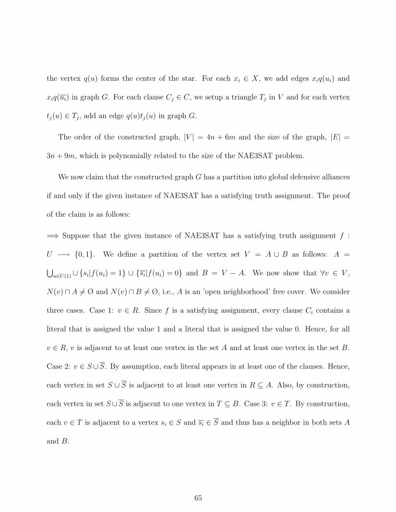
the vertex q(u) forms the center of the star. For each xi ∈ X, we add edges xiq(ui) and

xiq(ui) in graph G. For each clause Cj ∈ C, we setup a triangle Tj in V and for each vertex

tj(u) ∈ Tj, add an edge q(u)tj(u) in graph G.

The order of the constructed graph, |V | = 4n + 6m and the size of the graph, |E| =

3n + 9m, which is polynomially related to the size of the NAE3SAT problem.

We now claim that the constructed graph G has a partition into global defensive alliances

if and only if the given instance of NAE3SAT has a satisfying truth assignment. The proof

of the claim is as follows:

=⇒ Suppose that the given instance of NAE3SAT has a satisfying truth assignment f :

U −→ {0, 1}. We define a partition of the vertex set V = A ∪ B as follows: A =

⋃

u∈U(1) ∪{si|f(ui) = 1} ∪ {si|f(ui) = 0} and B = V − A. We now show that ∀v ∈ V ,

N(v) ∩A 6= Ø and N(v) ∩B 6= Ø, i.e., A is an ’open neighborhood’ free cover. We consider

three cases. Case 1: v ∈ R. Since f is a satisfying assignment, every clause Ci contains a

literal that is assigned the value 1 and a literal that is assigned the value 0. Hence, for all

v ∈ R, v is adjacent to at least one vertex in the set A and at least one vertex in the set B.

Case 2: v ∈ S ∪S. By assumption, each literal appears in at least one of the clauses. Hence,

each vertex in set S ∪ S is adjacent to at least one vertex in R ⊆ A. Also, by construction,

each vertex in set S∪S is adjacent to one vertex in T ⊆ B. Case 3: v ∈ T . By construction,

each v ∈ T is adjacent to a vertex si ∈ S and si ∈ S and thus has a neighbor in both sets A

and B.

65

⇐= Suppose now that the constructed graph G has an ’open neighborhood’ free cover A,

and let B = V − A. We define a truth assignment f : U −→ {0, 1}, such that f(ui) = 1

if and only if si ∈ A. Since each vertex ti ∈ T is adjacent to only two vertices, si ∈ S and

si ∈ S, exactly one of these vertices must be in set A. Thus, for each literal ui, f(ui) = 1 if

and only if f(ui) = 0, i.e., f is a legal assignment. Also, each vertex ri ∈ R has at least one

vertex in A and one vertex in B and hence each clause Ci has at least one true literal and

at least one false literal. Thus, f is a satisfying assignment. ¤

66

CHAPTER 4

ALLIANCE FREE AND ALLIANCE COVER SETS

4.1 Introduction

In this chapter, we introduce the concept of alliance-free and alliance cover sets, where

an alliance free set (for some type of alliance) is a set that does not contain any alliance

(of that type), while an alliance cover set (for some type of alliance) is a set that contains

at least one member (vertex) of each alliance (of that type). In particular, we consider the

alliance free and cover sets in the context of k−defensive and k−offensive alliances as defined

in Chapter 2.

Consider a graph G = (V,E) without loops or multiple edges. Recall that a vertex v in

set A ⊆ V is said to be k-satisfied with respect to A if degA(v) ≥ degV −A(v) + k, where

degA(v) = |N(v) ∩A| = |NA(v)| = deg(v) − degV −A(v). A set A is a defensive k-alliance if

all vertices in A are k−satisfied with respect to A, where −δ < k ≤ δ. Similarly, a set A ⊆ V

is an offensive k−alliance if ∀v ∈ ∂A, degA(v) ≥ degV −A(v) + k, where −δ + 2 < k ≤ δ.

67

A set X ⊆ V is defensive k−alliance free (k−daf) if for all defensive k−alliances A,

A − X 6= ∅, i.e., X does not contain any defensive k−alliance as a subset. A defensive

k−alliance free set X is maximal if ∀v /∈ X, ∃S ⊆ X such that S ∪ {v} is a defensive

k−alliance. A maximum k−daf set is a maximal k−daf set of largest cardinality. Let φk(G)

be the cardinality of a maximum k−daf set of graph G. For simplicity of notation, we will

refer to a maximum k−daf set of G as a φk(G)-set. If a graph G does not have a defensive

k−alliance (for some k), we say that φk(G)= |V (G)| = n, for example, φk(Pn)= n, ∀k > 1.

Since ∀k1 ≥ k2, a defensive k2−alliance free set is also defensive k1−alliance free, we have

φk1(G) ≥ φk2

(G) if and only if k1 ≥ k2.

We define a set Y ⊆ V to be a defensive k−alliance cover (k−dac) if for all defensive

k−alliances A, A∩Y 6= ∅, i.e., Y contains at least one vertex from each defensive k−alliance

of G. A k−dac set Y is minimal if no proper subset of Y is a defensive k−alliance cover. A

minimum k−dac set is a minimal cover of smallest cardinality. Let ζk(G) be the cardinality

of a minimum k−dac set of graph G. Once again, we will refer to a minimum k−dac set of

G as a ζk(G)-set. When G does not have a defensive k−alliance (for some k), we say that

ζk(G)= 0.

For offensive k−alliances, we define two types of alliance free (cover) sets depending on

whether or not the boundary vertices of an offensive alliance affect the definition of the

set. A set S ⊆ V is offensive k−alliance free (k−oaf) if for all offensive k−alliances A,

A − S 6= ∅. S is weak offensive k−alliance free (k−woaf) if for all offensive k−alliances A,

(A∪ ∂A)−S 6= ∅. Similarly, a set T ⊆ V is an offensive k−alliance cover (k−oac) if for all

68

offensive k−alliances A, A ∩ T 6= ∅. T is a weak offensive k−alliance cover (k−woac) if for

all offensive k−alliances A, (A ∪ ∂A) ∩ T 6= ∅. The maximum (weak) offensive k−alliance

free sets and minimum (weak) offensive k−alliance cover sets are defined in the same fashion

as their defensive counterparts. For a graph G, we define the following invariants

• φk(G) = Size of a maximum k−daf set of G

• ζk(G) = Size of a minimum k−dac set of G

• φok(G) = Size of a maximum k−oaf set of G

• ζok(G) = Size of a minimum k−oac set of G

• φwk (G) = Size of a maximum k−woaf set of G

• ζwk (G) = Size of a minimum k−woac set of G

In the remaining part of this chapter, we explore the properties and bounds of the above

defined invariants and their relationship with each other. In general we will refer to both

offensive and defensive k−alliances as k−alliances. Similarly, the terms k−alliance free set

and k−alliance cover set will encompass all types of alliance free sets and cover sets defined

in this section.

4.2 Basic Properties

We begin by presenting some basic properties of the alliance free sets and cover sets.

69

Theorem 60 X ⊆ V is a k−alliance cover if and only if V − X is k−alliance free.

Proof. A set X is a defensive k−alliance free set if and only if, for every defensive k−alliance

A, A − X 6= ∅ if and only if, for every defensive k−alliance A, A ∩ (V − X) 6= ∅ if and only

if V − X is a defensive k−alliance cover.

The justification for (weak) offensive alliance covers is similar. ¤

Corollary 61 φk(G)+ζk(G) = φok(G) + ζo

k(G) = φwk (G)+ζw

k (G) = n(G)

Corollary 62

(i) If V ′ is a minimal k-dac (k−oac) then, ∀v ∈ V ′, there exists a defensive (offensive)

k−alliance Sv for which Sv ∩ V ′ = {v}.

(ii) If V ′ is a minimal k-wdac then, ∀v ∈ V ′, there exists an offensive k−alliance Sv for

which (Sv ∪ ∂Sv) ∩ V ′ = {v}.

Since, ∀k1 > k2, a k2−alliance free set is also a k1−alliance free set and every k1−oaf set

is also a k1−woaf set, we have the following observation.

Observation 63 For any graph G and −∆ < k2 < k1 ≤ ∆,

(i) 0 ≤ φok2

(G) ≤ φok1

(G) ≤ φwk1

(G) ≤ n(G)

(ii) 0 ≤ φwk1

(G) ≤ φwk2

(G) ≤ n(G)

(iii) 0 ≤ φk2(G) ≤ φk1

(G) ≤ n(G)

70

Also note that every k−daf set X is also a k−woaf set. Suppose not, then there is

an offensive k−alliance A such that A ∪ ∂A ⊆ X. Then ∀v ∈ A′ = A ∪ ∂A, degA′(v) ≥

degV −A′(v) + k, which implies that A′ is a defensive k−alliance and contradicts X being a

k−daf set.

Observation 64 φwk (G) ≥ φk(G)

Suppose now a minimal k1−dac set Y , k1 > −δ(G), and let A ⊆ Y such that A is an

offensive k2−alliance. Let y ∈ A. Then by Corollary 62, there exists a defensive k1−alliance

Sy such that Sy ∩ Y = {y}. Hence ∃x ∈ ∂A − Y such that degA(x) ≤ degV −A(x) + 2 − k1.

Also, since A is an offensive k2−alliance, degA(x) ≥ degV −A(x) + k2. Combining the two

inequalities, we get, k2 ≤ 2 − k1. This leads to the following observation:

Observation 65 For any graph G and every k1, k2 such that k1 > −δ(G) and k2 > 2 −

k1, φok2

(G) ≥ ζk1(G)

4.3 Defensive k−Alliance Free & Cover Sets

For any k, such that −δ(G) < k ≤ ∆(G), we know that any independent set in a connected

graph G is k−daf, therefore φk(G) ≥ β0(G), where β0(G) is the vertex independence number

of graph G. We can further improve this bound by noting that the addition of any⌈

δ(G)2

⌉

+

⌊

k2

⌋

−1 vertices to an independent set will not produce a defensive k−alliance in the new set,

71

hence, φk(G) ≥ β0(G)+⌈

δ(G)2

⌉

+⌊

k2

⌋

−1. Since, every A ⊂ V , such that |A| ≥ n−⌊

δ(G)2

⌋

+⌈

k2

⌉

,

is a defensive k−alliance, φk(G) < n −⌊

δ(G)2

⌋

+⌈

k2

⌉

.

Observation 66 If G is a connected graph and −δ(G) < k ≤ ∆(G) then

β0(G) +

⌈

δ(G)

2

⌉

+

⌊

k

2

⌋

− 1 ≤ φk(G) < n −⌊

δ(G)

2

⌋

+

⌈

k

2

⌉

Next we present the values of φk(G) for some common graph families.

Observation 67 If G is an Eulerian graph and − δ(G)2

< i ≤ ∆(G)2

, then φ2i−1(G) = φ2i(G).

Observation 68 For the complete graph Kn and −n + 1 < k < n,

φk(Kn) =

⌊

n2

⌋

+⌈

k2

⌉

for odd n

⌊

n2

⌋

+⌊

k2

⌋

for even n.

Observation 69 For the complete bipartite graph Kp,q, where p ≤ q and −p < k ≤ p,

φk(Kp,q) =

q +⌈

p

2

⌉

+⌊

k2

⌋

− 1 for odd p

q +⌈

p

2

⌉

+⌈

k2

⌉

− 1 for even p.

Note that the upper and lower bounds of Observation 66 coincide for both Kn and Kp,q,

when k is even. We now show that for k ≥ 0, even complete graphs achieve the lower bound

for φk(G).

To show this, we first present a bound on φk(G) when k = 0. The result is then generalized

to k ≥ 0 in Theorem 78.

72

Theorem 70 If G is a connected graph then φ0 (G) ≥⌊

n2

⌋

.

Proof. Let A be a φ0 (G)−set of a connected graph G and assume, to the contrary, that

φ0 (G) <⌊

n2

⌋

. Let B = V (G) − A, hence |B| = ζ0 (G) >⌈

n2

⌉

. Since B is a 0−dac,

∀v ∈ B there exists a defensive 0−alliance S (v) such that S (v) ∩ B = {v}. Hence, ∀v ∈ B,

degA (v) ≥ degB (v). If B does not contain a defensive 0−alliance, then B is a 0−daf set,

which is contradiction since, |B| >⌈

n2

⌉

> φ0 (G). Hence, B must contain a minimal defensive

0− alliance T . If v ∈ T then degB (v) = degA (v). Hence, NB (T ) = T .

Suppose T is the only minimal defensive 0−alliance in B. Then, for any vertex x ∈ T ,

the set B − {x} is a defensive 0−alliance free set and |B − {x}| > φ0 (G), a contradiction.

Thus there are at least two disjoint defensive 0−alliances in B.

Now, assume that the number of disjoint minimal defensive 0−alliances in B is minimum

among all such sets. For each v ∈ B, let S (v) be a minimal defensive 0−alliance such that

S (v) ∩ B = {v}. Also, define:

D = {v ∈ B| degB (v) = degA (v)},

R = {v ∈ A| degA (v) = degB (v)},

R− = {v ∈ A| degA (v) < degB (v)}, and

R+ = {v ∈ A| degA (v) > degB (v)}.

Let T1, T2, . . . , Tr be the disjoint minimal defensive 0−alliances in B. By the above

arguments, r ≥ 2 and ∀i, NB (Ti) = Ti ⊆ D.

We now present a sequence of lemmas which culminate in the rest of the proof of Theo-

rem 70.

73

Lemma 71 For 1 ≤ i ≤ r and each x ∈ Ti, NA (x) ⊆ S (x) ∩ R−.

Proof. Suppose x ∈ Ti and let y ∈ NA (x). Since x ∈ Ti ⊆ D, degB (x) = degA (x). Hence,

NA (x) ⊆ S (x) and y ∈ S (x). Assume to the contrary that y /∈ R−, i.e., degA (y) ≥ degB (y).

Let A′ = A ∪ {x} − {y} and suppose S ′ ⊆ A′ is a defensive 0−alliance. Since degA′ (x) <

degB′ (x), x /∈ S ′. But, then S ′ ⊆ A, which contradicts A being 0−daf. Hence, A′ is defensive

0−alliance free and B′ = V −A′ is a 0−dac. Since Ti is a minimal defensive 0−alliance in B,

Ti − {x} is not a defensive 0−alliance in B′. Also, degB′ (y) < degA′ (y) implies that y /∈ T ′,

where T ′ is a defensive 0−alliance in B′. But then the number of disjoint minimal defensive

0−alliances in B′ is r− 1, which contradicts the assumption that B has a minimum number

of disjoint minimal defensive 0−alliances. ¤

Lemma 72 For i 6= j and every x1 ∈ Ti and x2 ∈ Tj, N (x1) ∩ N (x2) = ∅.

Proof. Suppose i 6= j and there exist x1 ∈ Ti and x2 ∈ Tj such that y ∈ N (x1) ∩ N (x2).

Since Ti ∩ Tj = ∅ and NB (Ti) = Ti, we have that y ∈ A. From Lemma 71, we know that

y ∈ R− ∩ S (x1)∩ S (x2). Consider the sets A′ = A∪ {x1, x2} − {y} and B′ = V −A′. Since

|A′| = |A| + 1 and A is a φ0 (G)−set, A′ must contain a defensive 0−alliance S ′. However,

degA (xl) = degB (xl), l ∈ {1, 2} and x1x2 /∈ E (G). Therefore, degA′ (xl) = degB′ (xl) − 1

and, hence, {x1, x2}∩S ′ = ∅. This implies that S ′ ⊆ A, and contradicts A being a defensive

0−alliance free set. ¤

Lemma 73 For every x ∈ Ti

(i) S (x) ⊆ NA (x) ∪ R ∪ {x} ,

74

(ii) S (x) is the unique minimal defensive 0−alliance in A ∪ {x} , and

(iii) NA∪{x} (S (x)) = S (x) .

Proof. Let x ∈ Ti and perform the following procedure:

S ′ ← NA (x) ∪ {x}

While NA (S ′) ⊆ NA (x) ∪ R and NA (S ′) − S ′ 6= ∅

Begin

S ′ ← S ′ ∪ NA (S ′)

End

Since G is finite, the procedure will terminate with either NA (S ′) − S ′ = ∅, or with a

vertex z ∈ NA (S ′) − S ′ such that z /∈ R. Assume NA (S ′) − S ′ 6= ∅. By construction,

S ′ ∪ NA (S ′) ∪ {z} ⊆ S (x) for every S (x) that is a defensive 0−alliance and for which

S (x) ∩ B = {x}. There are two cases.

Case 1. z ∈ R−: This implies that degA∪{x} (z) < degB−{x} (z) and contradicts the

assumption that S (x) is a defensive 0−alliance containing z.

Case 2. z ∈ R+: The set A′ = (A ∪ {x}) − {z} is a φ0 (G)−set, otherwise there is a

defensive 0−alliance in A ∪ {x} not containing z. Thus, B′ = V − A′ is a 0−dac. Since Ti

is a minimal defensive 0−alliance in B, Ti − {x} is not a defensive 0−alliance in B′. Also,

degB′ (z) < degA′ (z) implies that z /∈ T ′, where T ′ is a defensive 0−alliance in B′. But,

then the number of disjoint minimal defensive 0−alliances in B′ is r − 1, contradicting the

assumption that B has minimum number of disjoint minimal defensive 0−alliances.

75

Since both cases lead to a contradiction, we conclude that NA (S ′) − S ′ = ∅. Hence,

S ′ = S (x) ⊆ NA (x) ∪ R ∪ {x} and, by the construction, S (x) = S ′ is the unique minimal

defensive 0−alliance in A∪{x}. Also, since v ∈ S (x) implies degA∪{x}(v) = degB−{x}(v), we

must conclude that NA∪{x} (S (x)) = S (x). ¤

Lemma 74 For i 6= j and every x1 ∈ Ti and x2 ∈ Tj, S (x1) ∩ S (x2) = ∅.

Proof. Suppose i 6= j, x1 ∈ Ti, and x2 ∈ Tj. Assume, to the contrary, that z ∈ S (x1) ∩

S (x2). By Lemmas 71, 72 and 73, we know that NA (x1) ⊆ S (x1)∩R−, NA (x1)∩NA (x2) = ∅,

and S (x2) ⊆ NA (x2) ∪ R ∪ {x2}. Hence, NA (x1) ∩ S (x2) = ∅. Since S (x1) is a minimal

defensive 0−alliance, G [S (x1)], the subgraph of G induced by S (x1), is connected. Hence,

there is a path P in G [S (x1)] between z and a vertex y ∈ NA (x1) that does not contain x1.

From Lemma 73, NA∪{x2} (S (x2)) = S (x2) and, hence, y ∈ NA (x1)∩S (x2), a contradiction.

¤

Corollary 75 For i 6= j and any x1 ∈ Ti and x2 ∈ Tj, every path between S (x1) and S (x2)

contains a vertex not in A.

Lemma 76 If i 6= j then there is no path between Ti and Tj.

Proof. Assume to the contrary that such a path exists. Recall that Ti ∩ Tj = ∅ and

NB (Ti) = Ti. Hence, any path P from Ti to Tj must have an even number of edges in

common with the edge cutset 〈A,B〉. Let the number of common edges between the edge

cutset F = 〈A,B〉 and the path P be |F ∩ P | ≥ 2 and assume that |F ∩ P | is minimum for

all such bipartitions. Now we have two cases:

76

Case 1: |F ∩ P | = 2. Let F ∩ P = {x1a1, a2x2}, where x1 ∈ Ti, a1 ∈ NA (x1) ⊆ S (x1),

x2 ∈ Tj, and a2 ∈ NA (x2) ⊆ S (x2). By Lemma 74, S (x1)∩S (x2) = ∅ and, by Corollary 75,

there is no path from S (x1) to S (x2) consisting of only vertices in A, a contradiction.

Case 2: |F ∩ P | > 2. Let F ∩ P = {x1a1, a2x2, x3a3, . . . , a2s+2x2s+2}, s ≥ 1, where

x1 ∈ Ti, a1 ∈ NA (x1), a2 ∈ S (x1), x2 ∈ NB (a2), . . ., a2s+2 ∈ NA (x2s+2) and x2s+2 ∈ Tj.

Further, for 1 ≤ l ≤ 2s + 2, al ∈ A and xl ∈ B. We claim for 2 ≤ l ≤ 2s + 1, that xl /∈ Tu,

1 ≤ u ≤ r. Otherwise, suppose that xl ∈ Tu. Without loss of generality, assume u 6= i, then

there is a path from Ti to Tu such that |F ∩ P | ≤ 2s, which is contrary to P minimizing

|F ∩ P |.

Since a2 ∈ S (x1), by Lemma 73, the set A′ = A ∪ {x1} − {a2} is a φ0 (G)−set and the

set B′ = V − A′ is a 0−dac. Let F ′ = 〈A′, B′〉. Suppose there is no defensive 0−alliance

T ′ in B′ such that a2 ∈ T ′. Then there are r − 1 disjoint minimal defensive 0−alliances in

B′, which is a contradiction since B has the minimum number of disjoint minimal defensive

0−alliances. Thus, there is a defensive 0−alliance T ′ ⊆ B′ which contains a2 and is disjoint

from sets T1, . . . , Ti−1, Ti+1, . . . , Tk. But, then there is a path P ′ between T ′ and Tj such that

|F ′ ∩ P ′| = 2s, which is again a contradiction.

Since both cases lead to contradictions, there is no path P between Ti and Tj whenever

i 6= j. ¤

77

From Lemma 76, we conclude that G is disconnected, a contradiction. Therefore, the

set B must be defensive 0−alliance free and, hence, φ0 (G) ≥ |B| > |A| = φ0 (G), again a

contradiction. Thus, φ0 (G) ≥⌊

n2

⌋

, which completes the proof of Theorem 70. ¤

Corollary 77 If G is a connected Eulerian graph then φ−1 (G) ≥⌊

n2

⌋

.

In Chapter 5, we show that for connected graphs G, φ0(G) < ζ0(G) if and only if every

block of G is either an odd clique or an odd cycle.

Theorem 78 For every connected graph G and 0 ≤ k ≤ ∆, φk (G) ≥⌊

n2

⌋

+⌊

k2

⌋

.

Proof. By Theorem 70, the statement is true for k = 0. Since every k−daf set is also

(k + 1)−daf, φ1 (G) ≥ φ0 (G) ≥⌊

n2

⌋

=⌊

n2

⌋

+⌊

12

⌋

, i.e., the statement is also true for k = 1.

Hence, we may proceed by induction on k.

Assume that the statement is true for k ≤ M for arbitrary M > 1. Let A be a φM (G)−set

of a graph G. Again, A is also (M + 2)−daf of graph G. By the induction hypothesis,

φM+2 (G) ≥ |A| = φM (G) ≥⌊

n2

⌋

+⌊

M2

⌋

. If there exists a vertex v ∈ V −A such that A∪{v}

is (M + 2)−daf, then φM+2 (G) ≥ |A ∪ {v}| ≥⌊

n2

⌋

+⌊

M2

⌋

+ 1 =⌊

n2

⌋

+⌊

M+22

⌋

. Suppose no

such vertex exists. Then, ∀v ∈ V − A there exists a defensive (M + 2)−alliance S (v) such

that S (v) ∩ (V − A) = {v}. But, then ∀w ∈ S (v), degS(v)−{v} (w) ≥ degV −S(v)−{v} (w) + M

which is contrary to the assumption that A is M−daf. ¤

The bound of Theorem 78 is also sharp and is achieved by the complete graphs of even

order. We believe (but have been unable to prove) the following extension of the above

theorem:

78

Conjecture 79 If G is a connected graph and −δ(G) < k ≤ δ(G) then

φk(G) ≥⌊n

2

⌋

+

⌊

k

2

⌋

.

Next, we show that no forbidden subgraph characterization exists for the graphs induced

by minimal k−dac sets.

Theorem 80 Let G be any graph and r an integer such that r ≥ 2. Then, for all k ≥ 2− r,

there is a graph G′, such that G′ contains G as an induced subgraph and ζk(G′) = r.

Proof. Let a graph G = (V,E) where V = {v1, v2, . . . , vn} and construct a graph G′ =

(V ′, E ′) as follows: V ′ = V ∪X∪Y , where X ={

xji , 1 ≤ i ≤ n, 1 ≤ j ≤ max (2r + k, ∆(G) − k + 1)}

and Y = {y1, y2, . . . , y2r+k−2}. E ′ = E ∪ E1 ∪ E2, where E1 ={

vixji , vi ∈ V, xj

i ∈ X}

and E2 ={

xjiyl, xj

i ∈ X, yl ∈ Y}

. Thus δ(G′) = 2r + k − 1. Since by Observation 66,

ζk(G′) ≥

⌊

δ(G′)2

⌋

−⌈

k2

⌉

+ 1, we have ζk(G′) ≥

⌊

2r+k−12

⌋

−⌈

k2

⌉

+ 1 = r.

Now consider C ⊆ Y such that |C| = r. We claim that C is a k−dac set of graph G′.

Suppose not. Then there exists a defensive k−alliance S ⊆ V ′ − C in G′. Let v ∈ S. Since

∀x ∈ X, deg(x) = 2r + k − 1, if v ∈ X then degS(v) ≤ r + k − 1 < degC(v) + k = r + k,

which is contrary to S being a defensive k−alliance. Hence S ∩ X = ∅. Now let v ∈ V . By

construction of graph G′, ∀v ∈ V, degX(v)+k ≥ ∆(G)+1 > degV ′−X(v) ≥ degS(v), again a

contradiction. The only remaining case is S ⊂ Y , which is not possible as ∀v ∈ S, degS(v) =

0 < degV ′−S(y) + k ≤ n(2r + k) + k. Hence S = ∅ and C is a k−dac set. Thus ζk(G′) ≤ r.

Combining the two results, we get ζk(G′) = r. ¤

79

4.4 Offensive k−Alliance Free & Cover Sets

In this section, we study the properties of the free sets and cover sets associated with offensive

k−alliances. We begin by presenting the values of φok(G) and φw

k (G) for some special classes

of graphs.

Observation 81 For the complete graph Kn, and −n + 3 < k < n

φok(Kn) = φk(Kn) − 1 =

⌊

n + k

2

⌋

− 1

φwk (Kn) = n − 1

Observation 82 For the complete bipartite graph Kp,q, p ≤ q, and −p + 2 < k ≤ q

φok(Kp,q) =

⌈

q

2

⌉

+⌈

p

2

⌉

+ 2⌊

k2

⌋

− 2 p and q both odd

⌈

q

2

⌉

+⌈

p

2

⌉

+ 2⌈

k2

⌉

− 2 p and q both even

⌈

q

2

⌉

+⌈

p

2

⌉

+ k − 2 otherwise

φwk (Kp,q) = n − 2, p, q 6= 1

It is interesting to note that while complete graphs attain the lower bound for φk(G),

they have the maximum value for φwk (G).

Lemma 83 If S is an offensive k1− alliance then

80

(i) for all offensive k2−alliances S ′ ⊆ V − S such that k1 + k2 > 0, ∂S ∩ ∂S ′ = ∅.

(ii) for all defensive k2−alliances S ′ ⊆ V − S such that k1 + k2 > 0, ∂S ∩ S ′ = ∅.

Theorem 84 For a connected graph G, if X is a maximal k1−woaf set and Y = V − X

then

(i) ∀k2 > −k1, Y is a k2−woaf set (and hence, X is a k2−woac set), and

(ii) ∀k2 > max(−k1,−δ(G)), Y is a k2−daf set (hence, X is a k2−dac set).

Proof. For i), let k2 > −k1 and suppose there exists an offensive k2−alliance S for which

N [S] ⊆ Y . Let x ∈ ∂S. From Corollary 62, there is an offensive k1−alliance Sx for which

N [Sx] ∩ Y = {x}. If x ∈ ∂Sx, then from Lemma 83, S and Sx cannot be disjoint, a

contradiction. So we must assume that x ∈ Sx. But then, N(x) ⊆ ∂Sx ⊆ X, which leads to

a contradiction since x must have at least one neighbor in S ⊆ Y . Thus, Y is a k2−woaf set

and, from Theorem 60, X is a k2−woac set.

For ii), let k2 > max(−k1,−δ(G)) and suppose there exists a defensive k2− alliance

S ⊆ Y . Let x ∈ S. From Corollary 62, there exists an offensive k1− alliance Sx for which

N [Sx] ∩ Y = {x}. If x ∈ ∂Sx then from Lemma 83, S and Sx cannot be disjoint, a contra-

diction. So we must assume that x ∈ Sx, but then N(x) ⊆ ∂Sx ⊆ X, which is not possible

since degS(x) ≥ (deg(x) + k2)/2 > 0. Hence, Y is a k2−daf set and, from Theorem 60, X is

a k2−dac set. ¤

81

Corollary 85

(i) Every maximal k1−woaf set contains a minimal k2−woac set, ∀k2 > −k1.

(ii) Every maximal k1−woaf set contains a minimal k2−dac set, ∀k2 > max(−k1,−δ(G)).

Since every k−woaf is also l−woaf ∀l > k, by Theorem 60, every k−woac is also l−woac.

This observation leads to the following corollary of Theorem 84.

Corollary 86 ∀k > 0, ζwk (G) ≤

⌊

n2

⌋

It is easy to prove that ∀k ≥ 0, ζwk (G) =

⌊

n2

⌋

if and only if G ≈ K2 and k < 2.

We conclude this section by presenting a result for ζwk (G) similar to the one for ζk(G) in

Theorem 80.

Theorem 87 Let G be any graph and r an integer such that r ≥ 1. Then there is a graph

G′ with ζwk (G′) = r, which contains G as an induced subgraph.

Proof. Let a graph G = (V,E) where V = {v1, v2, . . . , vn} and construct a graph G′ =

(V ′, E ′) as follows: V ′ = V ∪ X ∪ Y , where X = {x1, x2, . . . , xr} and Y is the union of

disjoint sets Y1, Y2, . . . , Yr, such that ∀i, |Yi| = n−k +1. E ′ = E∪E1∪E2∪E3, where E1 =

{vixj, vi ∈ V, xj ∈ X}, E2 =⋃r

i=1 {xiy, ∀y ∈ Yi} and E3 = {yz| y, z ∈ Yi, 1 ≤ i ≤ r}.

Hence, G′ is obtained by adding r vertex disjoint cliques Yi ∪ {xi}, each of order n − k + 2

vertices and making each xi adjacent to every vertex of V .

It is easy to see that X is a k−woac set of graph G′, i.e. ζwk (G′) ≤ |X| = r. We claim

that ζwk (G′) = r. Suppose not and let C ⊂ V be a k−woac set of graph G′ such that |C| < r.

82

By pigeon hole principle, there exists Yi such that (Yi ∪{xi})∩C = ∅. Since ∂Yi = {xi} and

degYi(xi) = n+k+1 > degV ′−Yi

(xi)+k = n+k, Yi is an offensive k−alliance in G′ such that

N [Yi] ⊆ V ′ −C, which is contrary to C being a k−woac set of graph G′. Hence ζwk (G′) ≥ r.

Combining the two results, we get ζwk (G′) = r. ¤

83

CHAPTER 5

PARTITIONING A GRAPH INTO DEFENSIVE

0-ALLIANCE FREE (COVER) SETS

In this chapter, we deal with the problem of partitioning the vertex set of a graph G into

defensive 0-alliance free sets. We refer to such a partition as a defensive 0-alliance-free

partition and say G is partitionable if it has a defensive 0-alliance-free partition. Recall

from Chapter 3 that a partition is said to be unfriendly if each vertex has as many or more

neighbors outside the set in which it occurs than inside it. Note that, in an unfriendly

partition, if every vertex has strictly more neighbors outside the set in which it occurs than

inside it, then the partition is a defensive 0-alliance-free partition. However, the reverse is

not true, i.e., a vertex in a defensive 0-alliance free partition may have the same number of

neighbors inside the set in which it occurs than outside it.

As in the case for satisfactory partitions, not all the graphs have a defensive 0-alliance-

free partition. For example, odd cliques and odd cycles do not have defensive 0-alliance-free

partitions. In this chapter, we characterize graphs having defensive 0-alliance-free partitions.

In particular, we show the following:

84

Theorem 88 A connected graph G is partitionable if and only if G has a block that is other

than an odd clique or an odd cycle.

Define a set S to be a defensive 0-alliance free cover if S is both defensive 0-alliance free

and a defensive 0-alliance cover. Equivalently, S is a defensive 0-alliance free cover if for all

alliances X, X ∩ S 6= ∅ and X ∩ (V − S) 6= ∅. Thus, we have the following:

Lemma 89 A set S is a defensive 0-alliance free cover if and only if V − S is a defensive

0-alliance free cover.

From Lemma 89 and Theorem 60, we conclude the following:

Theorem 90 A graph G is partitionable if and only if G has a defensive 0-alliance free

cover.

5.1 When G is not Partitionable

We call a defensive 0-alliance cover X to be special if X contains exactly one minimal

defensive 0-alliance UX , such that:

1. ∀x ∈ UX , degX(x) = degV −X(x), i.e., NX(UX) = UX , and

2. ∀x ∈ UX , (V − X) ∪ {x} is also a special defensive 0-alliance cover.

85

It is shown in [SD02b] that if G does not have an defensive 0-alliance free cover then it has

a special defensive 0-alliance cover. Hence, from Theorem 90, if a graph is not partitionable,

it must contain a special defensive 0-alliance cover. The following lemma is immediate from

the definition of special defensive 0-alliance cover.

Lemma 91 If G is not partitionable and X is a special defensive 0-alliance cover in G then

for any x ∈ UX ⊆ X and y ∈ U(V −X)∪{x}, X ′ = (X − {x}) ∪ {y} is a special defensive

0-alliance cover, and y ∈ UX′.

Lemma 92 If G is not partitionable then for every v ∈ V (G), there exists a special defensive

0-alliance cover X such that the minimal defensive 0-alliance UX contains v.

Proof. Assume to the contrary, and let x ∈ V (G), such that for every special defen-

sive 0-alliance cover X, x /∈ UX . Let v ∈ UX be a nearest vertex to x. Also, let P =

v, v1, v2, . . . , vk, x be a shortest path from x to v. Since NX(UX) = UX , and P has minimum

length, v1 ∈ V −X. By the definition of special defensive 0-alliance cover, Y = (V − X)∪{v}

is a special defensive 0-alliance cover, and v1 ∈ UY , which is contrary to v being a nearest

such vertex to x. ¤

Corollary 93 If G is not partitionable, then G is Eulerian.

Proof. By definition of special defensive 0-alliance cover, if UX is the minimal defensive

0-alliance in an special defensive 0-alliance cover X, then ∀x ∈ UX , degX (x) = degV −X (x).

From Lemma 92, every vertex v ∈ V is in some such UX , hence, every vertex in G must have

even degree, i.e., Eulerian. ¤

86

The following theorem describes the partitionable graphs in terms of their blocks.

Theorem 94 A connected graph G is partitionable if and only if some block of G is parti-

tionable.

Proof. The proof is by induction on the number of blocks in graph G. The statement is

true if G is itself a block, and hence, the base case is true. Assume that the statement is

true for all graphs with at most r blocks, for a fixed but arbitrary r ≥ 1. Consider a graph

G with r +1 blocks and let x be a cut-vertex in G. Let G1 be the graph induced by V1 ⊂ V ,

where x ∈ V1 and V1 − {x} induces a connected component in graph G − {x}. Also, let G2

be the graph induced by V2 = (V − V1) ∪ {x}.

First, assume that G is partitionable and thus has a defensive 0-alliance free cover, say

B′. Further, assume that neither G1 nor G2 is partitionable. From Lemma 89, we may

assume that x ∈ B′. Note that for i ∈ {1, 2}, Bi = B′ ∩ Vi is defensive 0-alliance cover in

graph Gi. Thus each Bi must contain a defensive 0-alliance Ti in graph Gi. Now we have

two cases. Case 1: For some i ∈ {1, 2}, x /∈ Ti. Then, Ti ⊆ B′ is also a defensive 0-alliance in

graph G, which is contrary to B′ being a defensive 0-alliance free cover in graph G. Case 2:

x ∈ T1∩T2. But then, T1∪T2 ⊆ B′ is a defensive 0-alliance in graph G, again a contradiction.

Since both cases lead to a contradiction, we conclude that at least one of G1 and G2

is partitionable. Thus, by induction hypothesis, some block of G1 or G2 is partitionable.

Hence, some block of G is partitionable.

Next, suppose some block of G is partitionable. We may assume without loss of generality

that the block is in G1 and, hence, by the induction hypothesis, G1 is partitionable. Let B1

87

be a defensive 0-alliance free cover in G1. From Lemma 89, we may assume that x /∈ B1.

There are two cases. Case 1: G2 is partitionable. Then, there is a defensive 0-alliance free

cover B2 in G2. Once again, we may assume that x /∈ B2. But then B1 ∪ B2 is a defensive

0-alliance free cover of graph G, thus G is partitionable. Case 2: If G2 is not partitionable,

every defensive 0-alliance cover in G2 contains some defensive 0-alliance. By Lemma 92, there

exists a special defensive 0-alliance cover B2 in G2, such that x ∈ UB2. If B′ = (B1 ∪ B2)−{x}

is not a defensive 0-alliance cover of graph G then there must exist a defensive 0-alliance

S in G, such that S ∩ B′ = ∅ and x ∈ S. Since x ∈ UB2, |NV2∩S (x)| = |NV2−S (x)|. From

Corollary 93, we may assume that G is Eulerian, and |NV1(x)| ≥ 2, hence, V1 ∩ S 6= ∅ and

|NV1∩S(x)| ≥ |NV1−S(x)|. But then, V1 ∩ S is also a defensive 0-alliance in graph G1, which

contradicts B1 being a defensive 0-alliance cover in G1. Hence, B′ is a defensive 0-alliance

free cover of graph G, and G is partitionable. ¤

5.2 When a Block is Not Partitionable

From Theorem 94, a graph is not partitionable if and only if every block of G is not parti-

tionable. In this section, we characterize the blocks that are not partitionable.

Let G be a block that is not partitionable, and let X be a special defensive 0-alliance

cover in G containing a defensive 0-alliance UX . Also let Y = V − X.

Lemma 95 If a block G is not partitionable block then the graph G[UX ] is a block.

88

Proof. Assume to the contrary that x is a cut vertex in G[UX ]. Let {a, b} ⊆ UX , such that

every a− b path in G[UX ] contains x. Since G is a block, there must be a path P in G from

a to b that does not contain x. Since NX(UX) = UX , P ∩ 〈X,Y 〉 6= ∅. Assume now that the

choice of X, x, a and b is such that |P ∩ 〈X,Y 〉| is minimum among all such choices. Further,

assume that P is a shortest such path in G. Let P ∩ 〈X,Y 〉 = {y1y2, y3y4, . . . , y4k−1y4k} for

some k ≥ 1, where {y4i−3, y4i} ⊆ X and {y4i−2, y4i−1} ⊆ Y , 1 ≤ i ≤ k. In addition, y2j may

be the same as y2j+1, 0 < j < 2k. Since P is a shortest such path, y1 = a and y4k = b. Let

X0 = X and for 1 ≤ i ≤ k, define;

Xi = (Xi−1 − {y4i−3}) ∪ {y4i−1}, and

Yi = V − Xi.

From Lemma 91, ∀i, Xi is a special defensive 0-alliance cover. Also, ∀i > 0, {y4i−1, y4i, y4i+1} ⊆

UXiand y4i−1y4i ∈ E (G).

Let U ′ ⊆ UX0, such that G[U ′] is a connected component in G[UX0

− a] and b ∈ U ′. Note

that, ∀v ∈ U ′ − N(a), degU ′(v) = degV −U ′(v). In particular, degU ′(b) = degV −U ′(b). Now

there are two cases:

Case 1: Either k = 1 or for all j, 0 < j < k, U ′ ∩ UXj= ∅. Since b ∈ UXk

and

N(UXk) = UXk

, U ′ ⊆ UXk. But degU ′(b) = degV −U ′(b), and y4k−1b ∈ E(G) imply that

degXk(b) > degYk

(b), which is contrary to Xk being a special defensive 0-alliance cover.

Case 2: For some j, 0 < j < k, U ′ ∩ UXj6= ∅. Let j be the smallest such index.

Since, NXj(UXj

) = UXj, U ′ ⊆ UXj

. Since j < k and |P ∩ 〈X,Y 〉| is minimum, every

path in G[UXj] from y4j−1 to b must contain x. But then, x is a cut vertex in G[UXj

] and

89

|P ′ ∩ 〈Xj, Yj〉| < |P ∩ 〈X,Y 〉|, where P ′ ⊆ P is a path from y4j−1 to b that does not contain

x, a contradiction.

Since both cases lead to contradiction, we conclude that, G[UX ] is a block. ¤

Lemma 96 If G is not partitionable and {u, v} ⊆ UX , such that NV −X (u) ∩ NV −X (v) 6= ∅

then uv ∈ E(G).

Proof. Let {u, v} ⊆ UX , such that z ∈ NV −X (u) ∩ NV −X (v). By Lemma 91, X ′ =

(X − {u}) ∪ {z} is a special defensive 0-alliance cover, and z ∈ UX′ . Since v ∈ NX′ (z),

v ∈ UX′ , i.e., |NV −X′ (v)| = |NX′ (v)|, which is possible only if uv ∈ E (G). ¤

Lemma 97 If a block G is not partitionable and X is a special defensive 0-alliance cover

with |UX | > 2 then for any {a, b} ⊂ UX , NY (a) ∩ NY (b) 6= ∅, where Y = V − X.

Proof. Let |UX | > 2 and {a, b} ⊆ UX . From Lemma 95, ∀x ∈ UX , |NUX(x)| ≥ 2. Let

y2 ∈ NY (a). Since G is a block, there must exist a path P from y2 to b that does not

contain a. Let P be such a path, for which |P ∩ 〈X,Y 〉| is minimum among all such paths.

Let y1 = a and P ∩ 〈X,Y 〉 = {y3y4, y5y6, . . . , y4k−1y4k}, k ≥ 1, where {y4i−3, y4i} ⊆ X and

{y4i−2, y4i−1} ⊆ Y , 1 ≤ i ≤ k. Further, y2j may be the same as y2j+1, 0 < j < 2k. Also, let

y4k+1 = b, X0 = X and for 1 ≤ i ≤ k, define;

Xi = (Xi−1 − {y4i−3}) ∪ {y4i−1}, and

Yi = V − Xi.

From Lemma 91, ∀i, Xi is a special defensive 0-alliance cover. Also, ∀i > 0, {y4i−1, y4i, y4i+1} ⊆

UXiand y4i−1y4i ∈ E (G). Note that, ∀i, 0 < i < k, U ′∩UXi

= ∅, where U ′ = UX −{y1}, oth-

90

erwise, there is a y2− b path P ′ ⊆ P such that |P ′ ∩ 〈X,Y 〉| < |P ∩ 〈X,Y 〉|, a contradiction.

Since b ∈ UX2k, U ′ ⊆ UX2k

. Hence, ∀zi ∈ NUX(a), y4k−1zi ∈ E(G). Since |NUX

(a)| > 1, there

are at least two vertices z1, z2 in UX such that y4k−1 ∈ NY (z1) ∩ NY (z2). From Lemma 96,

z1z2 ∈ E(G).

We now claim that ∀x ∈ UX , y4k−1 ∈ N(x). Suppose not. Then there must exist

{u, v, w} ⊆ UX , such that {v, w} ⊆ N(u), and y4k−1 ∈ (N(u) ∩ N(v))−N(w). By Lemma 91,

X ′ = (X − {u}) ∪ {y4k−1} is a special defensive 0-alliance cover, and y4k−1 ∈ UX′ . Also,

since G[UX ] is a block and NX′(UX′) = UX′ , NX′(y4k−1) = NX(u), a contradiction. Hence,

∀x ∈ UX , y4k−1 ∈ N(x), which completes the proof. ¤

Theorem 98 If G is a block, then G is partitionable if and only if G is neither an odd clique

nor an odd cycle.

Proof. It is easy to see that odd complete graphs and odd cycles are not partitionable. To

prove the sufficiency of the theorem, let G be a block that is not partitionable and consider

two exhaustive cases:

Case 1: There exists an special defensive 0-alliance cover X in G, such that |UX | > 2.

Let Y = V −X. From Lemmas 96 and 97, G[UX ] is a clique, and ∀x ∈ UX , G[UY ∪{x}] is also

a clique. Hence ∀x ∈ UX , N [x] = UX ∪UY ∪{x}. Also, from the definition of special defensive

0-alliance covers, NY ∪{x}

(

UY ∪{x}

)

= UY ∪{x}. Thus, from Lemma 97, for every {x, y} ⊂ UX ,

N [x] = N [y]. By above arguments, ∀x ∈ UX , N [x] is a clique, and is a connected component

of the graph G. Since G is connected, this is only possible if G = G[N [x]]. Hence, G is a

complete graph. In addition, since even cliques are partitionable, G has odd order.

91

Case 2: For all special defensive 0-alliance covers X in G, |UX | = 2. From Lemma 91,

for all w ∈ V , there exists a special defensive 0-alliance cover B, such that w ∈ UB. Since,

|UB| = 2 and degUB(w) = degV −UB

(w), deg (w) = 2, and hence, G is a cycle. Further, since

even cycles are partitionable, G is an odd cycle. ¤

From Theorems 94 and 98, we conclude that a connected graph G is partitionable if and

only if G has a block that is other than an odd clique or an odd cycle, which is our main

result (Theorem 88).

For an Eulerian graph, a defensive 0-alliance free set is also a defensive (-1)-alliance free

set. Thus we have:

Corollary 99 An Eulerian graph G has a partition into defensive (-1)-alliance free sets if

and only if G has a block that is other than an odd clique or an odd cycle.

The characterization of graphs with defensive (-1)-alliance free partition is still an open

problem.

Also note that for k > 0, every unfriendly partition is a partition into defensive k-alliance

free sets. Therefore we have the following result.

Theorem 100 For k > 0, every graph G has a partition into defensive k-alliance free sets

and this partition can be found in polynomial time.

92

CHAPTER 6

GRAPH PARTITIONING AND DATA

CLUSTERING

6.1 Introduction

Clustering is a process of partitioning a set of data into clusters, where a cluster is a collection

of data points that are similar to each other and dissimilar to other data points. The problem

and its many variants have been studied extensively in mathematics as well as in applied

sciences. In the recent years, the availability of vast amounts of data (due to the emergence of

the world wide web, enormous increase in computing power, data storage and communication

speed) and the concept of data mining these massive databases has revitalized research on

the problem. Other than that, the clustering concepts are widely applied in the areas of

pattern recognition, machine learning and computer vision.

Different clustering algorithms use different concepts of cluster specific to the application

for which the algorithm is used. Moreover, sometimes the term cluster is implicitly defined by

the clustering criterion itself. In general, we define a set of clusters such that the similarities

93

of objects within each cluster as well as the dissimilarities of objects among the clusters

are maximized. Assume that the vertices in a graph are objects that we seek to group and

the edges (or weight of the edges) define the common property (similarity) that the objects

share. Clustering of these objects is then defined as a division of vertices into groups within

which the edges are dense, but between which they are sparser. This in turn implies that

the vertices in the groups have at least as many edges adjacent to the vertices inside the

group as to the vertices outside it. Recall from chapter 2 that a strong defensive alliance is

a set of vertices that have at least as many neighbors inside the set as they have outside it.

Thus, each cluster is a strong defensive alliance.

Once the definition of cluster is agreed upon, one can pose several interesting questions,

both of practical or theoretical natures. For example,

Q.1. How are the similarity measures to be defined? Similarity measures play an important

part in determining the quality of clustering. Different techniques demand different

types of measures, such as, measure of similarity between two objects, measure of sim-

ilarity between an object and a set of objects, and measure of similarity between two

sets of objects. Though similarity measures between objects are usually available for

the problem in hand, similarity measures between two sets, inter-cluster distances,

are hard to define. These distances are required by the clustering algorithms, which

proceed by merging smaller clusters with small inter-cluster distances ( Agglomera-

tive methods) and/or splitting large insufficiently similar clusters into smaller clusters

( Divisive methods). Standard inter-cluster distances include the distance between

94

the closest elements of the two clusters ( single-link clustering), the distance between

the farthest elements of the two clusters ( complete-link clustering), and the average

distance between the elements in the clusters ( group average clustering). For more

examples of inter-cluster distances, see [Mir96]

Q.2. What is the best choice for the numbers of clusters [Dub87, Bou99]? This fundamental

question in clustering is substantially hard to answer and is usually dodged by either i)

clustering the data for different choice of number of clusters and use the cluster validity

measures to decide which set of clusters best model the data, or ii) by generating

clusters as nested structures called Hierarchies. Given a data set S, a hierarchy is a set

H of subsets Sw ⊂ S, w ∈ W (where W is an index set), called clusters and satisfying

the following conditions: 1) S ∈ H and 2) for any S1, S2 ∈ H, S1 ∩ S2 ∈ {∅, S1, S2}.

Hence, a hierarchy of clusters consists of several levels, where the highest level contains

a single cluster (the whole data), and each data item is considered as a separate cluster

at the lowest level. A cluster in each intermediate level is partitioned by several clusters

at lower levels. The final choice of clustering is then decided by analyzing this hierarchy.

Both of these strategies lead to our next four questions.

Q.3. What is the measure of goodness of a given clustering [HA85, Dav79, BP98]?

Q.4. Can the given data be partitioned into k clusters (for some given k)? Of particular

interest is the special case, when k = 2 which provides the basis to most divisive clus-

tering algorithms. This problem is also known as Assessment of Clustering Tendency,

95

i.e., determining whether the data have structure in them or not without explicitly

looking for clusters in the data [JD88, Eve93b].

Q.5. What is the maximum k for which such a partitioning exist?

Q.6. Given that there is a partition of k clusters in a given data, what is the best such

clustering?

Q.7. Given k data items, is there a partition of k clusters, each containing one of the given

items?

Q.8. What are the upper and lower bounds on the size of a cluster? What are the charac-

teristics of extremal cases?

Q.9. Given a data item x, how many clusters contain x?

Q.10. How many clusters are there in a given data?

Q.11. What is the minimum size of a set containing at least one data item from each cluster?

Q.12. What is the maximum size of a set that does not contain any cluster?

In this chapter, we use strong defensive alliances as a model of clusters in the data.

With strong defensive alliance as the notion of cluster, the results presented in the previous

chapters are directly related to some of the questions posed above. The problem of assessment

of cluster tendency (Q.4), i.e., the existence of a bipartition into strong defensive alliances is

studied in Chapter 3. The maximum number of clusters (Questions 4, 5 and 12) is bounded

96

by the size of a minimum alliance cover of the graph (Chapter 4). The bounds on the size

of a cluster (Q. 8) are presented in Chapter 2. In this chapter, we present an algorithmic

solution for finding the clusters in a given data. Since the number of clusters are not known

in advance (Q. 2), the proposed algorithm generates a hierarchy of clusters by splitting each

cluster (starting with the cluster consisting of whole data) into two smaller clusters (strong

defensive alliances) until no cluster can be further partitioned.

Note that a given set of data may have many partitions into strong defensive alliances and

not every such partition is a good choice for generating a hierarchy of clusters. For example,

in the case of a disconnected graph with two connected components, the better choice for

the first bipartition is the one that divides the graph into two connected components, and

not the one that separates a strong defensive alliance from any of the components. This

problem is illustrated in Figure 6.1. In Figure 6.1(a), we first divide one of the connected

components into two strong defensive alliances and then proceed by further dividing the

generated clusters. In Figure 6.1(b), we first partition the graph into two components (strong

defensive alliances), and then proceed by further dividing the components. Even though the

final set of clusters is the same for both the cases, the hierarchies are not. In general, we

want the algorithm to generate the best division of data at every level of the hierarchy. It

is easy to see that at the first level of hierarchy, the partition of Figure 6.1(b) is a better

choice than the partition of Figure 6.1(a). The hierarchies of Figure 6.1 are represented in

the form of a tree or dendrogram in Figure 6.2.

97

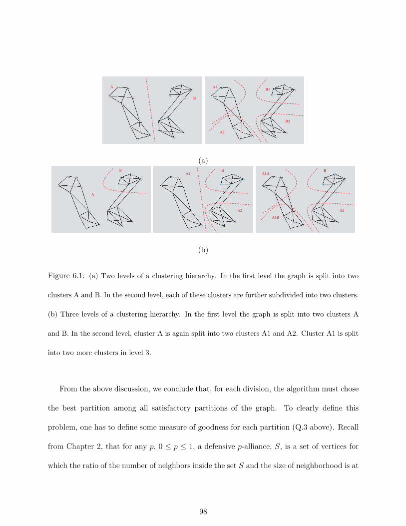
A

B

A

B

A1

B2

B1

A2

A1

B2

B1

A2

(a)

A

B

A

B B

A2

A1B

A2

A1 A1AB

A2

A1B

A1AB

A2

A1B

(b)

Figure 6.1: (a) Two levels of a clustering hierarchy. In the first level the graph is split into two

clusters A and B. In the second level, each of these clusters are further subdivided into two clusters.

(b) Three levels of a clustering hierarchy. In the first level the graph is split into two clusters A

and B. In the second level, cluster A is again split into two clusters A1 and A2. Cluster A1 is split

into two more clusters in level 3.

From the above discussion, we conclude that, for each division, the algorithm must chose

the best partition among all satisfactory partitions of the graph. To clearly define this

problem, one has to define some measure of goodness for each partition (Q.3 above). Recall

from Chapter 2, that for any p, 0 ≤ p ≤ 1, a defensive p-alliance, S, is a set of vertices for

which the ratio of the number of neighbors inside the set S and the size of neighborhood is at

98

A2 B2B1A1

BA

A2 B2B1A1 A2 B2B1A1

BA

A1B BA2A1A

A

A1

(a) (b)

Figure 6.2: The dendrograms (or hierarchical trees) of the hierarchies shown in Figure 6.1. The

leaves of the dendrogram represent the final clusters. As we move up the tree, the vertices join

together to form larger and larger clusters (indicated by horizontal lines). All these clusters are

joined together in a single group at the root of the tree.

least p, i.e., for all vertices v ∈ S, degS(v) ≥ p degV −S(v). Note that every strong defensive

alliance is a p-alliance, for some p ≥ 0.5. We define the measure of goodness of a partition of

strong defensive alliances, < A,B >, by the maximum value p ≤ 1, for which both A and B

are p-alliances. It is easy to see that the partition < A,B > of example in Figure 6.1(b) is

considered better than the partition < A,B > of Figure 6.1(a) by this measure. In the rest

of the chapter, we present an algorithm that finds a satisfactory partition of vertices that

maximizes this measure for all choices of satisfactory partitions of the given graph.

In the remainder of this chapter, we will assume the following notation.

In: unit matrix of order n × n.

en: n dimensional vector of all ones, i.e., en = [ 1 1 . . . 1 ]T .

99

A(i, j): element of ith row and jth column in the matrix A, A(i, j) = Aij

tr(A): trace of matrix A, i.e. sum of diagonal elements of matrix A.

A • B: matrix inner product, A • B = tr(

ATB)

Sn: set of all symmetric n × n matrices.

Mn: set of all n × n matrices.

S+n : set of all positive semidefinite matrices. A ∈ S+

n ⇔ A º 0

Diag(x): diagonal matrix with vector x as its diagonal.

diag(A): diagonal vector of the matrix A.

W: weight matrix of a weighted graph G. Wij is the weight of the edge between vertices vi

and vj.

The chapter is organized as follows: In Section 6.2, we review some existing graph theo-

retical clustering techniques. In Section 6.3, we present the details of the proposed algorithm.

In Section 6.4, we show the performance of the proposed algorithm on standard data sets.

Section 6.5 concludes the chapter.

6.2 Graph Theoretical Techniques for Clustering

The use of graph theoretical formalism to perform data clustering dates back to the 1950s.

The concept of a minimum spanning tree was initially used in clustering in a biologically

oriented method called Wrozlaw taxonomy [MM98]. Zahn [Zah71] also presented a clustering

method based on the minimum spanning tree (MST) of the dissimilarity graph (as opposed

100

to similarity graph). Urquhart [Urq82] used a similar approach along with normalization

of edge weight with respect to small neighborhood. Several other graph structures such as

cycles [SB94, Jac96, JI01, HW91], cliques [SB94] and shortest paths [SB94, CM98] have also

been used for finding clusters in data.

The simplest cluster definitions are formulated in terms of the threshold graphs Gt(Vt, Et),

where Vt = V and Et = {e ∈ E|w(e) ≥ t}. These clusters correspond to cliques, or compo-

nents of threshold graphs Gt. In 1959, Kuhn [Kuh59] defined the maximal complete subgraph

of a graph as a cluster. The same definition was applied in several of the classical clustering

algorithms [GK68] including the complete-link algorithm[JD88]. The definition is seen as

the strictest definition of a cluster [AM70, RY81] and its variants are still used in some clus-

tering applications [BY99]. Matula [Mat72] defined cluster as a maximal k−edge connected

subgraph, which he called k−components of graphs. A k−component is a maximal induced

subgraph G[S] with the property that for every partition 〈S1, S2〉 of S, at least k edges of

G[S] are each incident with a vertex of S1 and of S2. In [Bri02], a similar concept is applied to

define communities in a web-graph (internet-graph). In [Mat77], two other structures namely

k-bond and k-block were proposed. A k−bond is a maximal connected induced subgraph

G[S] where each vertex of S has degree at least k in the subgraph G[S]. The problem of

bi-partitioning of vertex set into sets constrained by their minimum degrees is addressed in

[Sti96, Tho83, Diw00, Kan98, Haj83]. A k−block is a maximal induced subgraph G[S] with

|S| ≥ k + 1 where G[S ′] is connected for any S ′ ⊂ S such that |S ′| ≥ |S| − k + 1.

101

A clump cluster is a set S ⊆ V such that, for every u, v ∈ S and a, b ∈ V − S,

w(u, v) > w(a, b). A strong cluster [Apr66, DF94] is a set S ⊆ V such that, for every

u, v ∈ S and a ∈ V − S, w(u, v) > max (w(a, u), w(a, v)). It can be seen that both clump

clusters and strong clusters form hierarchies of clusters. A weaker form of the above condition

defines weak clusters, where a set S ⊆ V is called a weak cluster if for all u, v ∈ S and

a ∈ V −S, w(u, v) > min (w(a, u), w(a, v)) [BD89]. Weak clusters form a weak hierarchy, i.e.,

for any weak clusters S1, S2, S3, S1 ∩ S2 ∩ S3 ∈ {∅, S1 ∩ S2, S2 ∩ S3, S3 ∩ S1}. A π−cluster

S ⊂ V is defined by the condition that d(S) ≥ π, where, d(S) =∑

u,v∈S

w(u,v)|S|2

is the average

similarity within S. A strict cluster is a set S ⊂ V such that for any a ∈ V − S and v ∈ S,

w(a, S) < w(S)2

≤ w(v, S), where w(a,S) is the average similarity of a and S and w(S) is the

average similarity of S.

The clumps and component clusters can be found by finding cliques and components in

graphs, while the other concepts are not as well developed.

Genkin and Muchnik [Gen93] defined the concept of t−clusters, where a set S ⊆ V is a

t−cluster or is a t−stable set if and only if the following conditions hold:

π (x, S) ≥ t for all x ∈ S

π (x, S) < t for all x ∈ V − S

where π (x, S) is the measure of similarity of data item x with respect to set S. It is shown

that many previously defined concepts of clusters, for example, cliques, k−components, and

k−blocks can be modelled in terms of t−clusters for different choices for π. The algorithms

for finding t−clusters also depends on this choice.

102

Recently, Pavan and Pelillo [PP03] proposed a generalization of the concept of maximal

clique to edge-weighted graphs based on the study of a continuous formulation of the max-

imum clique problem by Motzkin and Straus [MS65]. They termed the proposed structure

as dominant set. Let S ⊆ V be a non-empty subset of vertices and v ∈ V . The average

weighted degree of v w.r.t. S is defined as:

awdegS(v) =1

|S|∑

u∈S

w(u, v).

In addition, if u /∈ S, we define:

φS(u, v) = w(u, v) − awdegS(v).

Intuitively, φS(u, v) measures the similarity between vertices u and v, with respect to the

average similarity between vertex v and its neighbors in S. The weight of vertex v w.r.t. S

is

wS(v) =

1, if |S| = 1

∑

u∈S−{v} φS−{v}(u, v)wS−{v}(u), otherwise

Moreover, the total weight of set S is defined as:

W (S) =∑

v∈S

wS(v).

A non empty subset of vertices S ⊆ V such that W (T ) > 0 for any non-empty T ⊆ S is

said to be dominant if:

Q.1. wS(v) > 0, for all v ∈ S,

Q.2. wS∪{v}(v) < 0, for all v /∈ S.

103

The first condition corresponds to internal homogeneity of cluster while the second models

the external inhomogeneity. A quadratic programming approach was used to find dominant

sets in graphs.

The methods described above, first define a notion of what a cluster is, and then seek a

partition of the given data into the defined structure. Apart from these methods, various

kinds of graph partitioning problems define the clustering criterion without explicitly defining

a notion of cluster. Given a graph G, a partition P = 〈V1, V2, . . . , Vk〉 can be found by

minimizing or maximizing some global criterion. For example, maximizing within cluster

similarity:

f(P ) =k

∑

i=1

∑

u,v∈Vi

w(u, v)

|Vi|=

k∑

i=1

f(Vk).

Another possibility to model this problem is using minimum k−cuts, where a minimum

k−cut problem or k-way Split problem [GH88, HS85, SV91] is defined as follows: Given

an edge weighted graph G = (V,E) and an integer k, find a minimum weight set of edges

E ′ ⊆ E whose removal separates the graph into at least k nonempty connected components.

The problem is NP-hard for arbitrary k, while a polynomial algorithm exists for each fixed

k > 2, even for arbitrary graphs [GH88].

Another similar problem is called k−way cut or Multiway Cuts [DJP94], which is defined

as follows: Given an edge weighted graph G = (V,E), a set S = {s1, s2, . . . , sk} of k specified

vertices or terminals, find a minimum weight set of edges E ′ ⊆ E such that the removal of

E ′ from E disconnects each terminal from all the others. The problem is NP-Hard even for

104

k = 3; however it can be solved in polynomial time for planar graphs for any fixed k. The

planar problem is also NP-Hard for arbitrary k.

Due to the computational cost of the k−way partitioning problem, it is a usual practice to

approximate the general k−way partitioning solution by recursive bi-partitioning, where, at

each step, the graph is partitioned into two sets based on the partitioning criterion (though a

few exceptions exist, see, for example, [GWW01]). Finding a minimum 2-way cut or simply

minimum edge cutset is a polynomial problem [GH61]. As a matter of fact, all minimum cuts

in a graph can be generated in polynomial time [NNI97]. Wu and Leahy [WL93] proposed a

clustering method based on minimum edge cutset of graphs. The problem of finding k−way

partition was then approximated by recursively finding the minimum cuts that bisect the

existing clusters.

Though the minimum cut algorithm bi-partitions the graph in the optimal way, it has the

tendency to create very small clusters (i.e., the partitions formed are unbalanced in terms of

sizes of the sets). However, imposing constraints on the sizes of sets in the partition makes

the problem NP-Hard [WW91].

Shi and Malik [SM00] proposed the normalized cut measure for clustering, where the

normalized cut partitioning the vertex set V into sets A and B is defined as follows:

Ncut(A,B) =

∑

u∈A,v∈B w(u, v)∑

u∈A,t∈V w(u, t)+

∑

u∈A,v∈B w(u, v)∑

u∈B,t∈V w(u, t)

The problem is then to find a minimum normalized cut of graph G. The problem of

finding a minimum normalized cut is NP-Hard and an approximate algorithm known as

105

spectral clustering is applied to find the solution. Perona and Freeman [PF98] proposed an

asymmetric variation of normalized cut, which they referred to as foreground cut. Define

one of the two subsets of G to be a foreground F and its complement B = V − F to be the

background, then the foreground cut N(F ) is given as:

N(F ) =

∑

u∈F,v∈B w(u, v)∑

u∈F,t∈F w(u, t)

Once again, a minimum foreground cut is sought in the graph. Sarkar and Soundararajan

[SS00] also used a graph partition based framework and normalized the edge cutset by the

product of the sizes of each partition and referred to as average cut. Both of these problems

are again NP-Hard and can be approximated by spectral clustering.

Similar ideas of partitioning the vertex set of graphs using some global criterion are

employed in [Vek00, Wan01, KVV00, IG98, Wei99, YS01].

6.3 Clustering Using Maximum Satisfactory Minimum Cut

6.3.1 Problem Definition

In this section, we present the details of the proposed algorithms. As mentioned in Sec-

tion 6.1, that given a graph G = (V,E), we seek a bipartition of the vertex set V into sets

A,B, such that both A and B are defensive p-alliances and p is maximum among all such

bipartitions. In the case, when there is more than one such partition, we find one which

106

has the minimum number of edges between the sets A and B. We refer to such a cut as

a maximum satisfactory minimum cut of the graph G. Formally, we define the problem as

follows:

MAXIMUM SATISFACTORY MINIMUM CUT (MSMC)

Input: A Graph G(V,E) and a weight function w : E → R.

Question: Find a partition A,B of V and a real number p, 0 ≤ p ≤ 1, such that,

i. for all v ∈ A,∑

u∈N(v)∩A w(u, v) ≥ p∑

u∈N(v) w(u, v),

ii. for all v ∈ B,∑

u∈N(v)∩B w(u, v) ≥ p∑

u∈N(v) w(u, v),

iii. p is maximum among all partitions, A,B, satisfying (i) and (ii).

iv. The cut between sets A and B is minimum among all the partitions satisfying (i),(ii)

and (iii).

The above problem is NP-Hard (By reduction from Satisfactory Partition). In order to

find an approximate solution of the above problem, we start by first presenting a quadratic

programming formulation of MSMC. Let V = {v1, v2, . . . , vn}. For each vertex vi ∈ V , we

define a binary variable xi. We want to find a partition, A,B, of V into defensive p-alliances,

A = {vi|xi = 0} and B = {vi|xi = 1} such that p is maximum among all such partitions. A

partition A,B of V is a satisfactory p-partition (a partition into defensive p-alliances, if and

only if for every vertex vi,

107

−∑

vj∈N(vi)

w(vi, vj) ≤ p(2xi − 1)∑

vj∈N(vi)

w(vi, vj) −∑

vj∈N(vi)

xjw(vi, vj) ≤ 0

We also want both sets A and B to be nonempty. As a matter of fact, for the sets A

and B to be strong defensive alliances, each of them must have at least 2 vertices. Thus, we

must have∑n

i=1 xi ≥ 2 and∑n

i=1 xi ≤ n − 2.

The complete quadratic program can now be written as follows:

Maximize: Kp − ∑

1≤i<j≤n w(vi, vj)(xi − xj)2

Subject to the following constraints:

• p(2xi − 1)∑

vj∈N(vi)w(vi, vj) −

∑

vj∈N(vi)xjw(vi, vj) ≤ 0, 1 ≤ i ≤ n

• p(2xi − 1)∑


∑

vj∈N(vi)xjw(vi, vj) ≥ −∑

vj∈N(vi)w(vi, vj), 1 ≤ i ≤ n

• x2i = xi, 1 ≤ i ≤ n

• ∑n

i=1 xi ≥ 2

• ∑n

i=1 xi ≤ n − 2

• p ≥ 0

• p ≤ 1

The second term,∑

1≤i<j≤n w(vi, vj)(xi−xj)2 in the objective function is the value of the

cut and minimizing it corresponds to maximizing the objective function. On the other hand,

the increase in the value of p increases the term Kp and hence, the objective function. Here,

K is a constant that controls the precision of calculating p and should be chosen such that

108

the increase in the value of p by the amount of required precision has more effect on the value

of objective function than the value of any of the cut. In general, K À ∑

1≤i<j≤n w(vi, vj).

The functional and constraints of the above quadratic program have the form of a general

quadratic functional, i.e., xTQx + 2bTx. We can homogenize this program by introducing

a new variable x0 and setting it to 1. We may then replace each linear term axi by the

quadratic term axix0. Thus, the homogenous version of the above quadratic program can

be written as:

Maximize: Kpx0 −∑

1≤i<j≤n w(vi, vj)(xi − xj)2

Subject to the following constraints:

• p(2xi − x0)∑


∑

vj∈N(vi)xjx0w(vi, vj) ≤ 0, 1 ≤ i ≤ n

• p(2xi − x0)∑


∑

vj∈N(vi)xjx0w(vi, vj) ≥ −∑

vj∈N(vi)w(vi, vj), 1 ≤ i ≤ n

• x2i = xix0, 1 ≤ i ≤ n

• ∑n

i=1 xix0 ≥ 2

• ∑n

i=1 xix0 ≤ n − 2

• px0 ≥ 0

• px0 ≤ 1

• x20 = 1

109

6.3.2 Semidefinite Relaxation of MSMC

The quadratic program given in the previous subsection is equivalent to MSMC prob-

lem, and hence, is NP-Hard. We now present a semidefinite relaxation of this quadratic

program. Semidefinite programming is linear programming over the cone of semidefinite

matrices[WSV00, LS91]. In comparison to standard linear programming the vector x ∈ Rn

of variables is replaced by a matrix variable X ∈ S+n , where S+

n is the set of all n×n positive

semidefinite matrices. In other words, the cone of the nonnegative orthant x ≥ 0 is replaced

by the cone of semidefinite matrices X º 0. A semidefinite program is an optimization

problem of the following form:

Maximize A0 • X

subject to Ai • X = ci, 1 ≤ i ≤ m, X º 0

where X ∈ Mn and for all 0 ≤ i ≤ m, Ai ∈ Mn.

The trick to obtain a polynomially solvable relaxation of the quadratic programming

problems (as defined in the previous subsection), is to think of each variable xi as vectors

in a higher dimensional space Rk, and subsequently, multiplications of two vectors as inner

product in this space [Hel00]. Different choices of the dimension k < n (where n is the number

of variables of the quadratic program of concern) of this new space provides different problems

of geometric nature, but usually are still NP-Hard. However, if we chose the dimension of

the new space to be equal to the number of original variables then we get a polynomial time

110

solvable problem. Using this technique, we may write a polynomially solvable relaxation of

the quadratic program of previous subsection as follows:

Maximize: KpTx0 −∑

1≤i<j≤n w(vi, vj)(xi − xj)T (xi − xj)

• pT (2xi − x0)∑


∑

vj∈N(vi)xT

j x0w(vi, vj) ≤ 0, 1 ≤ i ≤ n

• pT (2xi − x0)∑

vj∈N(vi)w(vi, vj)−

∑

vj∈N(vi)xT

j x0w(vi, vj) ≥ −∑

vj∈N(vi)w(vi, vj), 1 ≤

i ≤ n

• xTi xi = xT

i x0, 1 ≤ i ≤ n

• ∑n

i=1 xTi x0 ≥ 2

• ∑n

i=1 xTi x0 ≤ n − 2

• pTx0 ≥ 0

• pTx0 ≤ 1

• xT0 x0 = 1

In order to derive a semidefinite relaxation of the above homogenous quadratic program

of the form xTQx, we note the fact that xTQx = Q•xxT and replace xxT with a matrix X to

come up with a linear objective function. The variables of this new system are the elements

of matrix X. Imposing the condition that X º 0, i.e., X is a semidefinite matrix gives

us a semidefinite program. The inequalities in the constraints are replaced with equalities

by introducing slack variables (one for each inequality). These steps yield the following

111

semidefinite program for the MSMC problem that consists of 3n + 6 variables (including

2n + 4 slack variables) and 3n + 6 constraints.

Maximize A0 • X

X =

X1 0

0 L

∈ S3n+6, where X1 = xxT , x = [ x1 x2 . . . xn p x0 ]T and L is a diago-

nal matrix whose diagonal is the vector of 2n+4 slack variables, i.e., L = Diag(

[ l1 l2 . . . l2n+4 ]T)

.

A0 =

B1 0 0

0 B2 0

0 0 0

, where B1 = W − Diag (Wen), and B2 =

0 K2

K2

0

.

Constraints:

• X º 0

• Ai • X = 0, 1 ≤ i ≤ n.

i. Ai(i, n + 1) = Ai(n + 1, i) =∑

vj∈N(vi)w(vi, vj)

ii. for all j 6= i, 1 ≤ j ≤ n, Ai(j, n + 2) = Ai(n + 2, j) = −12w(vi, vj),

iii. Ai(n + 1, n + 2) = Ai(n + 2, n + 1) = −12

∑

vj∈N(vi)w(vi, vj), and

iv. Ai(n + i + 2, n + i + 2) = 1.

• Ai • X = −∑

vj∈N(vi−n) w(vi−n, vj), n + 1 ≤ i ≤ 2n.

i. Ai(i − n, n + 1) = Ai(n + 1, i − n) =∑

vj∈N(vi−n) w(vi−n, vj)

ii. for all j 6= (i − n), 1 ≤ j ≤ n, Ai(j, n + 2) = Ai(n + 2, j) = −12w(vi−n, vj),

112

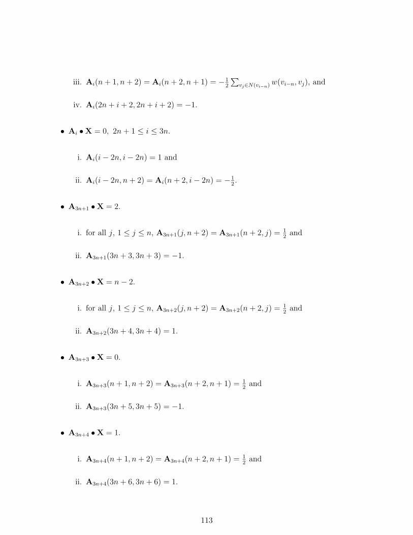
iii. Ai(n + 1, n + 2) = Ai(n + 2, n + 1) = −12

∑

vj∈N(vi−n) w(vi−n, vj), and

iv. Ai(2n + i + 2, 2n + i + 2) = −1.

• Ai • X = 0, 2n + 1 ≤ i ≤ 3n.

i. Ai(i − 2n, i − 2n) = 1 and

ii. Ai(i − 2n, n + 2) = Ai(n + 2, i − 2n) = −12.

• A3n+1 • X = 2.

i. for all j, 1 ≤ j ≤ n, A3n+1(j, n + 2) = A3n+1(n + 2, j) = 12

and

ii. A3n+1(3n + 3, 3n + 3) = −1.

• A3n+2 • X = n − 2.

i. for all j, 1 ≤ j ≤ n, A3n+2(j, n + 2) = A3n+2(n + 2, j) = 12

and

ii. A3n+2(3n + 4, 3n + 4) = 1.

• A3n+3 • X = 0.

i. A3n+3(n + 1, n + 2) = A3n+3(n + 2, n + 1) = 12

and

ii. A3n+3(3n + 5, 3n + 5) = −1.

• A3n+4 • X = 1.

i. A3n+4(n + 1, n + 2) = A3n+4(n + 2, n + 1) = 12

and

ii. A3n+4(3n + 6, 3n + 6) = 1.

113

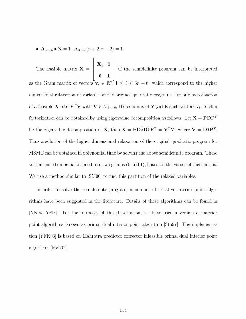
• A3n+5 • X = 1. A3n+5(n + 2, n + 2) = 1.

The feasible matrix X =

X1 0

0 L

of the semidefinite program can be interpreted

as the Gram matrix of vectors vi ∈ Rn, 1 ≤ i ≤ 3n + 6, which correspond to the higher

dimensional relaxation of variables of the original quadratic program. For any factorization

of a feasible X into VTV with V ∈ M3n+6, the columns of V yields such vectors vi. Such a

factorization can be obtained by using eigenvalue decomposition as follows. Let X = PDPT

be the eigenvalue decomposition of X, then X = PD1

2D1

2PT = VTV, where V = D1

2PT .

Thus a solution of the higher dimensional relaxation of the original quadratic program for

MSMC can be obtained in polynomial time by solving the above semidefinite program. These

vectors can then be partitioned into two groups (0 and 1), based on the values of their norms.

We use a method similar to [SM00] to find this partition of the relaxed variables.

In order to solve the semidefinite program, a number of iterative interior point algo-

rithms have been suggested in the literature. Details of these algorithms can be found in

[NN94, Ye97]. For the purposes of this dissertation, we have used a version of interior

point algorithms, known as primal dual interior point algorithm [Stu97]. The implementa-

tion [YFK03] is based on Mahrotra predictor corrector infeasible primal dual interior point

algorithm [Meh92].

114

6.4 Results

6.4.1 Zachary’s Karate Club Network

Wayne Zachary [Zac77] observed social interactions between the members of a karate club at

an American university in the early 1970s for two years. The data consists of the ties between

members of the club based on their social interactions with each other and is shown in

Figure 6.31. He used these data and an information flow model of network conflict resolution

to explain the split-up of this group following disputes among the members. The split-up

of the group occurred after the dispute between the administrator and the principal karate

teacher. In Figure 6.3, we show the partition obtained by our algorithm for this network.

The administrator and the instructor are represented by vertices 1 and 33 respectively. The

vertices in each cluster are shown using different color. From ground truth, we find that only

vertex 3 is incorrectly classified by our algorithm, the rest of the split found by the algorithm

is consistent with the actual split of the club. Also, from the figure it is clear that the vertex

3 has equal number of ties with both clusters and its assignment to any cluster cannot be

justified by the given data and hence, must be made arbitrarily. The final clustering of the

data is shown in Figure 6.4, where a total of 3 clusters were detected.

1The networks shown in this chapter are drawn using Pajek[BM98]

115

Figure 6.3: The network of ties between the members of the karate club from Zachary Karate

Club data set. The bipartition of the data generated by our algorithm is shown by using different

colors for the members belonging to different clusters. The members with greater ties with the

administrator (vertex 1) are colored blue whereas the members with greater ties with the instructor

(vertex 33) are colored yellow. Only the coloring of vertex 3 is inconsistent with the actual split of

the club.

6.4.2 Zoo Database

Zoo Database was created by David Forsyth (PC/BEAGLE User’s Guide) and contains the

data of 101 animals. The entry for each animal consists of 15 binary attributes, such as,

whether or not the animal has fins, feathers, hairs, etc, or if the animal lays eggs, or is

116

Figure 6.4: Final clustering of the Zachary Karate Club data generated by the proposed algorithm.

venomous. There is also one numeric attribute that provides the number of legs for each

animal. Some properties of the database are listed in Table 6.1.

We defined the dissimilarity between two animals as the hamming distance between their

binary feature vector (Though legs is a numeric feature, it only takes five discrete values

and can be converted into as many binary features). The edge weights of the graph were

then defined as the number of binary features minus the hamming distance between the two

feature vectors. This graph was used as an input to our algorithm. Our algorithm found

11 groups in the data (this happened because some of the groups in the data set had the

tendency for further subdivision and is not considered an error on the part of algorithm).

The groups obtained by the algorithm are shown in Figure 6.5. The same information

117

is also presented in tabular form in Table 6.2. The class hierarchy is shown in the form

of dendrogram in Figure 6.6. From these results, it can be clearly seen that the clusters

generated by the algorithm are quite consistent with the actual classification of Table 6.1.

Figure 6.5: Grouping among the animals of zoo database. A total of 9 groups were recognized by

the algorithm.

118

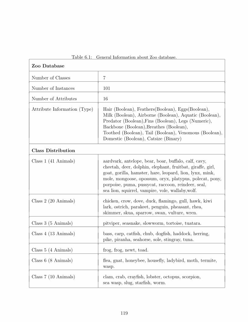
Table 6.1: General Information about Zoo database.

Zoo Database

Number of Classes 7

Number of Instances 101

Number of Attributes 16

Attribute Information (Type) Hair (Boolean), Feathers(Boolean), Eggs(Boolean),Milk (Boolean), Airborne (Boolean), Aquatic (Boolean),Predator (Boolean),Fins (Boolean), Legs (Numeric),Backbone (Boolean),Breathes (Boolean),Toothed (Boolean), Tail (Boolean), Venomous (Boolean),Domestic (Boolean), Catsize (Binary)

Class Distribution

Class 1 (41 Animals) aardvark, antelope, bear, boar, buffalo, calf, cavy,cheetah, deer, dolphin, elephant, fruitbat, giraffe, girl,goat, gorilla, hamster, hare, leopard, lion, lynx, mink,mole, mongoose, opossum, oryx, platypus, polecat, pony,porpoise, puma, pussycat, raccoon, reindeer, seal,sea lion, squirrel, vampire, vole, wallaby,wolf.

Class 2 (20 Animals) chicken, crow, dove, duck, flamingo, gull, hawk, kiwilark, ostrich, parakeet, penguin, pheasant, rhea,skimmer, skua, sparrow, swan, vulture, wren.

Class 3 (5 Animals) pitviper, seasnake, slowworm, tortoise, tuatara.

Class 4 (13 Animals) bass, carp, catfish, chub, dogfish, haddock, herring,pike, piranha, seahorse, sole, stingray, tuna.

Class 5 (4 Animals) frog, frog, newt, toad.

Class 6 (8 Animals) flea, gnat, honeybee, housefly, ladybird, moth, termite,wasp.

Class 7 (10 Animals) clam, crab, crayfish, lobster, octopus, scorpion,sea wasp, slug, starfish, worm.

119

Table 6.2: Clusters of animals in the Zoo database as found by the proposed algorithm.

Number of Classes 11

Class Distribution

Class 1 (2 Animals) aardvark, bear.

Class 2 (30 Animals) antelope, boar, buffalo, calf, cavy, cheetah, deer, elephant,giraffe, goat, hamster, hare, leopard, lion, lynx, mink, mole,mongoose, opossum, oryx, platypus, polecat, pony, puma,cat, raccoon, reindeer, sea lion, vole, wolf.

Class 3 (6 Animals) fruitbat, girl, gorilla, squirrel, vampire, wallaby.

Class 4 (3 Animals) dolphin, porpoise, seal

Class 5 (14 Animals) bass, carp, catfish, chub, dogfish, haddock, herring,pike, piranha, seahorse, sea snake, sole, stingray, tuna.

Class 6 (21 Animals) chicken, crow, dove, duck, flamingo, gull, hawk, kiwilark, ostrich, parakeet, penguin, pheasant, rhea,skimmer, skua, sparrow, swan, tortoise, vulture, wren.

Class 7 (8 Animals) frog, frog, newt, pitviper, scorpion, slowworm, toad, tuatara.

Class 8 (2 Animals) flea,termite.

Class 9 (6 Animals) gnat, honeybee, housefly, ladybird, moth, wasp

Class 10 (5 Animals) crab, crayfish, lobster, octopus, starfish.

Class 11 (4 Animals) clam, sea wasp, slug, worm.

120

Class 1

Class 3

Class 2

Class 9

Class 8

Class 7

Class 6

Class 5

Class 4

Class 11

Class 10

Figure 6.6: Dendrogram of the clusters obtained by the proposed algorithm.

6.4.3 Networks of Fictional Characters

In this subsection, we present results on two data sets based on the ties between the fictional

characters. The first data set provides the ties between different characters of Victor Hugo’s

novel Les Miserables, whereas the other provides the same for Mark Twain’s Huckleberry

Finn. Compiled by Knuth[Knu93] as part of the Stanford GraphBase project, the data

sets define the ties between two characters based on whether or not the two ever appeared

in the same scene. Our algorithm found 10 clusters of (more than one) characters of Les

Miserables, that are shown in Figure 6.7. The clusters generated are consistent with the

121

different subplots of the novel. We compare the clusters obtained by our algorithm to the

ones achieved by Newman and Girvan [NG04], in Table 6.4.3. A total of 9 groups were found

among the characters of Huckleberry Finn (Figure 6.8). The algorithm correctly recognized

the family structure of Grangerfords and also the network of Phelps. The other dominant

groups are centered around the main characters Tom Sawyer, slave Jim, Doctor Robinson

and Duke.

6.4.4 Other Standard Data Sets

In addition to the social structure networks of previous data sets, we also tested our algorithm

on five other standard data sets for classification algorithms. These data sets are Wine, Iris

Plant, Hepatitis, Dermatology Database, and Protein Localization Sites. (Some facts about

these databases are summarized in Tables 6.4-6.8. We also compare the performance of our

algorithm on these data sets with the performance of normalized cut algorithm by Shi and

Malik[SM00].

The first data set, Wine Recognition Data (Table 6.4) consists of the results of a chemical

analysis of wines grown in the same region in Italy but derived from three different cultivars.

The analysis determined the quantities of 13 constituent found in each of the three types

of wines. There are a total of 178 samples of wines in the data set, 59 belonging to class

1, 71 of class 2 and 48 of class 3. When run over the complete data set, our algorithm

correctly classifies all the samples of first and third class, however 9 samples of the class

122

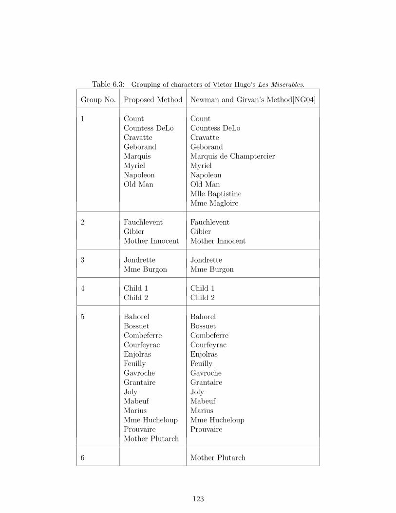
Table 6.3: Grouping of characters of Victor Hugo’s Les Miserables.

Group No. Proposed Method Newman and Girvan’s Method[NG04]

1 Count CountCountess DeLo Countess DeLoCravatte CravatteGeborand GeborandMarquis Marquis de ChamptercierMyriel MyrielNapoleon NapoleonOld Man Old Man

Mlle BaptistineMme Magloire

2 Fauchlevent FauchleventGibier GibierMother Innocent Mother Innocent

3 Jondrette JondretteMme Burgon Mme Burgon

4 Child 1 Child 1Child 2 Child 2

5 Bahorel BahorelBossuet BossuetCombeferre CombeferreCourfeyrac CourfeyracEnjolras EnjolrasFeuilly FeuillyGavroche GavrocheGrantaire GrantaireJoly JolyMabeuf MabeufMarius MariusMme Hucheloup Mme HucheloupProuvaire ProuvaireMother Plutarch

6 Mother Plutarch

123


7 Baroness T Baroness TGillenormand GillenormandLt Gillenormand Lt GillenormandMlle Gillenormand Mlle GillenormandMlle Vaubois Mlle VauboisMme Pontmercy Mme Pontmercy

CosetteOld Woman 2MagnonToussaint

8 BoulatruelleCosetteMagnonOld woman 2ToussaintAnzelma AnzelmaBabet BabetBrujon BrujonClaquesous ClaquesousEponine EponineGueulemer GueulemerJavert JavertMme Thenardier Mme ThenardierMontparnasse MontparnassePontmercy PontmercyThenardier Thenardier

9 Boulatruelle

124


10 Blacheville BlachevilleDahlia DalhiaFameuil FameuilFantine FantineFavourite FavouriteListolier ListolierFelix Tholomyes Felix TholomyesZephine Zephine

MargueritePerpetue

11 Mlle BaptistinePerpetueMme MagloireMargueriteGervais GervaisIsabeau IsabeauLabarre LabarreMme De R Mme De ROld Woman 1 Old Woman 1Scaufflaire ScaufflaireSimplice SimpliceJean Valjean Jean Valjean

BamataboisBrevetChampmathieuChenildeiuCockepailleJudge

12 BamataboisBrevetChampmathieuChenildeiuCockepailleJudge

125

Table 6.4: General information about Wine Recognition database.

Data Set: Wine Recognition



Attributes alcohol, malic acid, ash, alcalinity of ash, magnesium,total phenols, flavanoids, nonflavanoid phenols,proanthocyanins, color intensity, hue,OD280/OD315 of diluted wines, proline

Class Distribution Class 1: 59 instancesClass 2: 71 instancesClass 3: 48 instances

Table 6.5: General information about Iris Plant data set

Data Set: Iris Plant



Attributes sepal length, sepal width, petal length, petal width

Class Distribution Class 1 (Iris Setosa): 50 instancesClass 2 (Iris Versicolour): 50 instancesClass 3 (Iris Virginica): 50 instances

126

Table 6.6: General information about Hepatitis data set

Data Set: Hepatitis



Attributes age, sex, steroid, antivirals, fatigue, malaise, anorexia,liver big, liver firm, spleen palpable, spiders, ascites, varices,bilirubin, alk phosphate, sgot, albumin, protime, histology

Class Distribution Class 1 (Live): 123 instancesClass 2 (Die) : 32 instances

Table 6.7: General information about Dermatology data set

Data Set: Dermatology



Class Distribution Class 1 (psoriasis): 112 instancesClass 2 (seboreic dermatitis): 61 instancesClass 3 (lichen planus): 72 instancesClass 4 (pityriasis rosea): 49 instancesClass 5 (cronic dermatitis): 52 instancesClass 6 (pityriasis rubra pilaris) : 20 instances

127

Figure 6.7: Grouping among the characters of Victor Hugo’s Les Miserables. A total of 10 groups

were recognized by the algorithm excluding the three groups that only contain one character each,

which form the connected components of the network

2 were incorrectly classified, 6 were assigned to class 1 and 3 to class 2. On the other

hand, normalized cut algorithm was unable to correctly classify 36 members of class 2 and

1 member of class 3, thus providing the classification accuracy of 79.21% as compared to

94.94% accuracy of Maximum Satisfactory Minimum Cut (MSMC) algorithm. We also

128

Figure 6.8: Nine groups that were found by the proposed algorithm among the characters of Mark

Twain’s Huckleberry Finn

tested the algorithm by using the data points of only two of the classes at a time. The

algorithm MSMC algorithm classified 97.69% of data points belonging to class 1 and 2. The

classification accuracy values between class 2 and class 3 and between class 1 and class 3

were 97.48% and 100% respectively. For the same data, the classification accuracy values for

129

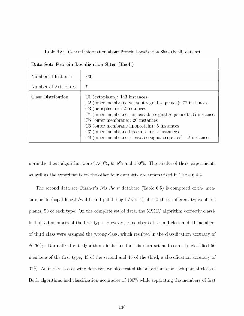
Table 6.8: General information about Protein Localization Sites (Ecoli) data set

Data Set: Protein Localization Sites (Ecoli)



Class Distribution C1 (cytoplasm): 143 instancesC2 (inner membrane without signal sequence): 77 instancesC3 (perisplasm): 52 instancesC4 (inner membrane, uncleavable signal sequence): 35 instancesC5 (outer membrane): 20 instancesC6 (outer membrane lipoprotein): 5 instancesC7 (inner membrane lipoprotein): 2 instancesC8 (inner membrane, cleavable signal sequence) : 2 instances

normalized cut algorithm were 97.69%, 95.8% and 100%. The results of these experiments

as well as the experiments on the other four data sets are summarized in Table 6.4.4.

The second data set, Firsher’s Iris Plant database (Table 6.5) is composed of the mea-

surements (sepal length/width and petal length/width) of 150 three different types of iris

plants, 50 of each type. On the complete set of data, the MSMC algorithm correctly classi-

fied all 50 members of the first type. However, 9 members of second class and 11 members

of third class were assigned the wrong class, which resulted in the classification accuracy of

86.66%. Normalized cut algorithm did better for this data set and correctly classified 50

members of the first type, 43 of the second and 45 of the third, a classification accuracy of

92%. As in the case of wine data set, we also tested the algorithms for each pair of classes.

Both algorithms had classification accuracies of 100% while separating the members of first

130

class from the other two. The classification accuracy of MSMC algorithm between class 2

and class 3 was 80% compared to 88% of normalized cut algorithm.

Similar experiments were performed for other three data sets. Other than the iris plant

data set, MSMC algorithm consistently provided better accuracy than normalized cut. The

results are presented in Table 6.4.4.

6.5 Conclusion

Clustering is still a developing field and is far from solved. The models and algorithms are

neither general enough to be applicable to a variety of problems nor is there much consensus

of which models to be used in which problems and why. This is because of the arbitrariness of

the choice of models and the difficulty of independent interpretation of them outside the given

applications. In addition, most of the models lead to NP-Hard problems and that requires a

search for efficient approximate algorithms preferably with lower bounds on errors. Alliance

is an intuitive model for clusters, groups or communities in a network. Using this model,

we defined an objective function that is maximized by the optimal grouping of the vertices

(in terms that the within group similarities and intergroup dissimilarities are maximized).

We also presented an approximate algorithm to find such a grouping. We showed by using

real world data that the algorithm performs well and is also comparable to other competing

algorithms.

131

Table 6.9: Comparison of MSMC Algorithm and Normalized Cut Algorithm

Data Set Input Domain Classification Performance

MSMC Algorithm Normalized Cut Algorithm

Wine Class 1: 59 instants Class 1: 59/59 Class 1: 59/59Recognition Class 2: 71 instants Class 2: 62/71 Class 2: 35/71

Class 3: 48 instants Class 3: 48/48 Class 3: 47/48

Accuracy: 94.94% Accuracy: 79.21%

Class 1: 59 instants Class 1: 59/59 Class 1: 58/59Class 2: 71 instants Class 2: 68/71 Class 2: 69/71



Accuracy: 100% Accuracy: 100%



Iris Class 1: 50 instants Class 1: 50/50 Class 1: 50/50Plant Class 2: 50 instants Class 2: 41/50 Class 2: 43/50

Class 3: 50 instants Class 3: 39/50 Class 3: 45/50

Accuracy: 86.66% Accuracy: 92%







132

Data Set Input Domain Classification Performance

MSMC Algorithm Normalized Cut Algorithm

Hepatitis Class 1: 32 instants Class 1: 30/32 Class 1: 30/32Class 2: 123 instants Class 2: 65/123 Class 2: 55/123


Dermatology Class 1: 112 instants Class 1: 112/112 Class 1: 112/112Class 4: 49 instants Class 4: 49/49 Class 4: 49/49



Accuracy: 100% Accuracy: 95.45%





Protein Class 2: 77 instants Class 2: 75/77 Class 2: 70/77Localization Class 4: 52 instants Class 4: 48/52 Class 4: 50/52

Sites (Ecoli) Accuracy: 95.35% Accuracy: 93.02%

133

List of References

[AM70] J. G. Augustson and J. Minker. “An Analysis of Some Graph Theoretical ClusterTechniques.” Journal of the Association for Computing Machinery, 17(4):571–588, October 1970.

[AMP90] R. Aharnoi, E. C. Milner, and K. Prikry. “Unfriendly partitions of a graph.”Journal of Combinatorial Theory Series B, 50:1–10, 1990.

[And73] M. R. Anderberg. Cluster Analysis for Applications. Academic Press, 1973.

[Apr66] Y. Apresian. “An algorithm for finding clusters by a distance matrix.” ComputerTranslation and Applied Linguistics, 9:72–79, 1966.

[BD89] H. J. Bandelt and A. W. M. Dress. “Weak hierarchies associated with similaritymeasures-an additive clustering technique.” Bulletin of Mathematical Biology,51:133–166, 1989.

[BDH02] R. C. Brigham, R. D. Dutton, T. W. Haynes, and S. T. Hedetniemi. “Powerfulalliances in graphs.” Preprint, 2002.

[BDH04] R. C. Brigham, R. D. Dutton, and S. T. Hedetniemi. “Secure alliances.” Preprint,2004.

[Ber87] C. Bernardi. “On a theorem about vertex coloring of graphs.” Discrete Mathe-matics, 64(1):95–96, 1987.

[BHJ93] P. J. Bernhard, S. T. Hedetniemi, and D. P. Jacobs. “Efficient sets in graphs.”Discrete Applied Mathematics, 44:99–108, 1993.

[BK] O. V. Borodin and A. V. Kostochka. “On an upper bound of a graph’s chromaticnumber, depending on the graph’s degree and density.” Journal of CombinatorialTheory Series B, 23:247–250.

[BM98] V. Batagelj and A. Mrvar. “Pajek - Program for Large Network Analysis.”Connections, 21(1):47–57, 1998.

[Bou99] A. O. Boudraa. “Dynamic estimation of number of clusters in data sets.” Elec-tronic Letters, 35(19):1606–1608, 1999.

134

[BP98] J. C. Bezdek and N. R. Pal. “Some new indexes of cluster validity.” IEEETrasactions on Systems, Man, and Cybernetics, 28(3):301–315, June 1998.

[Bri02] M. Brinkmeier. “Communities in Graphs.” Technical report, TU Ilmenau, 2002.

[BTV03a] C. Bazgan, Zs. Tuza, and D. Vanderpooten. “Complexity of the satisfactory par-tition problem.” Algorithmic Discrete Mathematics Technical Report 34, LAM-SADE, December 2003.

[BTV03b] C. Bazgan, Zs. Tuza, and D. Vanderpooten. “On the existence and determinationof satisfactory partitions in a graph.” In ISAAC 2003, LNCS 2906, pp. 444–453,2003.

[BY99] A. Ben-Dor and Z. Yakhini. “Clustering gene expression patterns.” In Proceed-ings of the Third Annual International Conference on Computational MolecularBiology, 1999.

[CBD04] A. Cami, H. Balakrishnan, N. Deo, and R. Dutton. “On the complexity of someglobal alliance problems.” In Eighteenth Midwest Conference on Combinatorics,Cryptography and Computing, 2004.

[CE] R. Cowan and W. Emerson. “Proportional coloring of graphs, unpublished.”.

[CM98] S. Casadei and S. K. Mitter. “Hierarchical Image Segmentation Detection ofRegular Curves in a Vector Graph.” International Journal of Computer Vision,27(1):71–100, 1998.

[Dav79] D. L. Davies. “A cluster separation measure.” IEEE Transactions on PatternAnalysis and Machine Intelligence, 1(4):224–227, 1979.

[DF94] J. Diatta and B. Fichet. “From Apresian hierarchies and Bandelt Dress weakhierarchies to quasi-hierarchies.” In E. Diday, Y. Lechevallier, M. Shader,P. Bertrand, and B. Burtschy, editors, New Approaches in Classification andData Analysis, pp. 111–118. Springer, 1994.

[DGH96] J. E. Dunbar, W. Goddard, S. T. Hedetniemi, M. A. Henning, and A. A. McRae.“The algorithmic complexity of minus domination in graphs.” Discrete Mathe-matics, 168:73–84, 1996.

[DH] R. O. Duda and P. E. Hart. Pattern Classification and Scene Analysis. Wiley-interscience, New York.

[DHH95a] J. E. Dunbar, F. Harris, S. M. Hedetniemi, S. T. Hedetniemi, R. Laskar, andA. McRae. “Nearly perfect sets in graphs.” Discrete Mathematics, 138:229–246,1995.

135

[DHH95b] J. E. Dunbar, S. T. Hedetniemi, M. A. Henning, and P. J. Slater. “Signed domi-nation in graphs.” In Y. Alavi and A. J. Schwenk, editors, Proc. 7th InternationalConferrence on Combinatorics, Graph Theory, Applications, pp. 311–322. Wiley,1995.

[DHH96] J. E. Dunbar, S. T. Hedetniemi, M. A. Henning, and A. A. McRae. “Minusdomination in regular graphs.” Discrete Mathematics, 149:311–312, 1996.

[DHH99] J. E. Dunbar, S. T. Hedetniemi, M. A. Henning, and A. A. McRae. “Minusdomination in graphs.” Discrete Mathematics, 199:35–47, 1999.

[DHL00] J. E. Dunbar, D. G. Hoffman, R. C. Laskar, and L. R. Markus. “α-Dominationin graphs.” Discrete Mathematics, 211:11–26, 2000.

[Diw00] A. A. Diwan. “Decomposing graphs with girth at least five under degree con-straints.” Journal of Graph Theory, 33:237–239, 2000.

[DJP94] E. Dahlhaus, D. S. Johnson, C. H. Papadimitriou, P. D. Seymour, and M. Yan-nakakis. “The Complexity of Multiterminal Cuts.” SIAM Journal of Computing,23:864–894, 1994.

[Dub87] R. C. Dubes. “How many clusters are best?- An experiment.” Pattern Recogni-tion, 20:645–663, 1987.

[Eve93a] B. Everitt. Cluster Analysis. Edward Arnold, London, 1993.

[Eve93b] B. Everitt. Graphical Techniques for Multivariate Data. North Holland, NewYork, 1993.

[Fav94] O. Favaron. “Signed domination in graphs.” Discrete Mathematics, 125:147–152,1994.

[FFG02] O. Favaron, G. Fricke, W. Goddard, S. M. Hedetniemi, S. T. Hedetniemi, P. Kris-tiansen, R. C. Laskar, and D. Skaggs. “Offensive alliances in graphs.” Preprint,2002.

[FLG00] G. W. Flake, S. Lawrence, and C. L. Giles. “Efficient identification of Web com-munities.” In Proc. 6th ACM SIGKDD International Conference on KnowledgeDiscovery and Data Mining, Boston, MA, 2000.

[FLH] G. H. Fricke, L. M. Lawson, T. W. Haynes, S. M. Hedetniemi, and S. T. Hedet-niemi. “A note on defensive alliances in graphs.” Bulletin ICA, to appear.

[FP03] D. A. Forsyth and J. Ponce. Computer Vision: A Modern Approach. PrenticeHall, NJ, 2003.

136

[Gen93] A. V. Genkin. “Fixed points approach to clustering.” Journal of Classification,10:219–240, 1993.

[GH61] R. E. Gomory and T. C. Hu. “Multi-terminal network flows.” SIAM Journal ofApplied Mathematics, 9:551–570, 1961.

[GH88] O. Goldschmidt and D. S. Hochbaum. “Polynomial algorithm for the k−cut prob-lem.” In Proc. 29th Annual Symposium on Foundations of Computer Science, pp.444–451, Los Angeles, California, 1988. IEEE Computer Society.

[GK68] C. C. Gotlieb and S. Kumar. “Semantic clustering of index terms.” Journal ofthe Association for Computing Machinery, 15(4):493–513, 1968.

[GK00] M. U. Gerber and D. Kobler. “Algorithmic approach to the satisfactory graphpartitioning problem.” European Journal of Operational Research, 125:283–291,2000.

[GK01] M. U. Gerber and D. Kobler. “Partitioning a graph to satisfy all vertices.”Technical Report, Swiss Federal Institute of Technology,Lausanne, 2001.

[GWW01] Y. Gdalyahu, D. Weinshall, and M. Werman. “Self organization in vision:Stochastic clustering for image segmentation, perceptual grouping, and imagedatabase organization.” IEEE Transactions on Pattern Analysis and MachineIntelligence, 23(10):1053–1074, 2001.

[HA85] L. J. Hubert and P. Arabie. “Comparing partitions.” Journal of Classification,2:193–218, 1985.

[Haj83] P. Hajnal. “Partition of graphs with condition on the connectivity and minimumdegree.” Combinatorica, 3:95–99, 1983.

[Har75] J. A. Hartigan. Clustering Algorithms. John Wiley and sons, 1975.

[Hel00] C. Helmberg. “Semidefinite Programming for Combinatorial Optimization.” Jan-uary 2000.

[HHH02] T. W. Haynes, S. T. Hedetniemi, and M. A. Henning. “Global defensive alliancesin graphs.” Preprint, 2002.

[HHK00] S. M. Hedetniemi, S. T. Hedetniemi, and P. Kristiansen. “Alliances in graphs.”Preprint, 2000.

[HHS94] J. H. Hattingh, M. A. Henning, and P. J. Slater. “Three-valued k-neighbourhooddomination in graphs.” Australas. Journal of Combinatorics, 9:233–242, 1994.

137

[HHS95] J. H. Hattingh, M. A. Henning, and P. J. Slater. “On the algorithmic complexityof signed domination in graphs.” Australas. Journal of Combinatorics, 12:101–112, 1995.

[Hop82] J.J. Hopfield. “Neural networks and physical systems with emergent collectivecomputational abilities.” Proc. National Academy of Science, 79:2254–2258,1982.

[HS85] D. S. Hochbaum and D. B. Shmoys. “An O(|V |2) algorithm for the planar 3-cutproblem.” SIAM Journal of Algebraic and Discrete Methods, 6:707–712, 1985.

[HW91] D. P. Huttenlocher and P. C. Wayner. “Finding convex edge groupings in animage.” In Proc. IEEE Conference of Computer Vision and Pattern Recognition,pp. 406–412, 1991.

[IG98] H. Ishikawa and D. Geiger. “Segmentation by grouping junctions.” In Proc.IEEE Conference of Computer Vision and Pattern Recognition, 1998.

[Jac96] D. W. Jacobs. “Robust and efficient detection of salient convex groups.” IEEETransactions on Pattern Analysis and Machine Intelligence, 18(1):23–37, Jan-uary 1996.

[JD88] A. K. Jain and R. C. Dubes. Algorithms for Clustering Data. Prentice Hall,Englewood Cliffs, NJ, 1988.

[JI01] I. H. Jermyn and H. Ishikawa. “Globally optimal regions and boundaries as min-imum ratio weight cycles.” IEEE Transactions on Pattern Analysis and MachineIntelligence, 23(10):1075–1088, October 2001.

[Kan98] A. Kaneko. “On decomposition of triangle-free graphs under degree constraints.”Journal of Graph Theory, 27:7–9, 1998.

[Knu93] D. E. Knuth. The Stanford GraphBase: A Platform for Combinatorial Comput-ing. Addison-Wesley, Reading, MA, 1993.

[Kuh59] J. L. Kuhns. “Mathematical analysis of correlation clusters.” In Word correlationand automatic indexing, Progress Rep. No. 2. Ramo-Wooldridge, Canoga Park,California, 1959.

[KVV00] R. Kannan, S. Vempala, and A. Vetta. “On clusterings-good, bad and spectral.”In Proc. 41st Annual Symposium on Foundations of Computer Science, 2000.

[Lan04] L. Langley. “Alliances in Directed Graphs.” In 35th Southeastern InternationalConference on Combinatorics, Graph Theory, and Computing, March 2004.

[LS91] L. Lovasz and A. Schrijver. “Cones of matrices and set-functions and 0-1 opti-mization.” SIAM Journal of Optimization, 1(2):166–190, 1991.

138

[Lub86] M. Luby. “A simple parallel algorithm for the maximum independent set prob-lem.” SIAM Journal of Computing, 15:1036–1053, 1986.

[Mat72] D. W. Matula. “k-components, clusters, and slicing in graphs.” SIAM Journalof Applied Mathematics, 22:459–480, 1972.

[Mat77] D. W. Matula. “Graph Theoretic Cluster Analysis.” In J. V. Ryzin, editor,Classification and Clustering. 1977.

[Meh92] S. Mehrotra. “On the implementation of a primal-dual interior point method.”SIAM Journal on Optimization, 2:575–601, 1992.

[MGH02] A. McRae, W. Goddard, S. M. Hedetniemi, S. T. Hedetniemi, and P. Kristiansen.“The algorithmic complexity of alliances in graphs.” Preprint, 2002.

[Mir96] B. Mirkin. Mathematical Classification and Clustering. Kluwer academic pub-lishers, 1996.

[MM98] B. Mirkin and I. Muchnik. “Combinatorial Optimization in Clustering.” In D. Z.Du and P. M. Pardalos, editors, Handbook of Combinatorial Optimization. KluwerAcademic Publishers, 1998.

[MS65] T. S. Motzkin and E. G. Straus. “Maxima for graphs and a new proof of a theormof Turan.” Canadian Journal of Mathematics, 17:533–540, 1965.

[NG04] M. E. J. Newman and M. Girvan. “Finding and Evaluating Community Structurein Networks.” Phys. Rev. E., 69, 2004.

[NN94] Y. Nesterov and A. Nemirovskii. “Interior-point polynomial algorithms in convexprogramming.” SIAM Studies in Applied Mathematics, 1994.

[NNI97] H. Nagamochi, K. Nishimura, and T. Ibaraki. “Computing all small cuts in anundirected network.” SIAM Journal of Discrete Mathematics, 10:469–481, 1997.

[PF98] P. Perona and W. Freeman. “A factorization approach to grouping.” Proc.European Conference on Computer Vision, pp. 655–670, 1998.

[PP03] M. Pavan and M. Pelillo. “A new graph-theoretic approach to clustering and seg-mentation.” In IEEE Conference of Computer Vision and Pattern Recognition,June 2003.

[RY81] V. V. Raghavan and C. T. Yu. “A comparison of the stability characteristicsof some graph theoretical clustering methods.” IEEE Transactions on PatternAnalysis and Machine Intelligence, 3:393–402, 1981.

139

[SB94] S. Sarkar and K. L. Boyer. “A computational structure for preattentive percep-tual organization: Graphical enumeration and voting methods.” IEEE Transac-tions on Systems, Man, and Cybernetics, 24(2):246–267, 1994.

[SD02a] K. H. Shafique and R. D. Dutton. “On satisfactory partitioning of graphs.”Congressus Numerantium, 154:183–194, 2002.

[SD02b] K. H. Shafique and R. D. Dutton. “A tight bound on the cardinalities of maxi-mum alliance-free and minimum alliance-cover sets.” Preprint, 2002.

[SD03] K. H. Shafique and R. D. Dutton. “Maximum Alliance-Free and MinimumAlliance-Cover Sets.” In 34th Southeastern International Conference on Com-binatorics, Graph Theory, and Computing, March 2003.

[SD04] K. H. Shafique and R. D. Dutton. “Partitioning a graph into Alliance-free Sets.”Preprint, 2004.

[SM90] S. Shelah and E. C. Milner. “Graphs with no unfriendly partitions.” In A. Baker,B. Bollobas, and A. Hajnal, editors, A tribute to Paul Erdos, pp. 373–384. Cam-bridge University Press, 1990.

[SM00] J. Shi and J. Malik. “Normalized Cuts and Image Segmentation.” IEEE Trans-actions on Pattern Analysis and Machine Intelligence, 22(8):888–905, August2000.

[Sok77] R. R. Sokal. “Clustering and Classification: Background and Current Direc-tions.” In J. V. Ryzin, editor, Classification and Clustering. 1977.

[SS00] S. Sarkar and P. Soundararajan. “Supervised learning of large perceptual organi-zation: Graph spectral partitioning and learning automata.” IEEE Transactionson Patterm Analysis and Machine Intelligence, 22(5):504–525, May 2000.

[Sti96] M. Stiebitz. “Decomposing graphs under degree constraints.” Journal of GraphTheory, 23:321–324, 1996.

[Stu97] J. F. Sturm. “Primal-Dual interior point approach to semidefinite programming.”Tinbergen institute research series, vol. 156, Erasmus University Rotterdam, Rot-terdam Netherlands, 1997.

[SV91] H. Saran and V. V. Vazirani. “Finding k−cuts within twice the optimal.” InProc. 32nd Annual Symposium on Foundations of Computer Science, pp. 743–751, Los Angeles, California, 1991. IEEE Computer Society.

[SY91] A. A. Schaffer and M. Yannakakis. “Simple local search problems that are hardto solve.” SIAM Journal of Computing, 20:56–87, 1991.

140

[Tho83] C. Thomassen. “Graph decomposition with constraints on the connectivity andminimum degree.” Journal of Graph Theory, 7:165–167, 1983.

[Urq82] R. Urquhart. “Graph theoretical clustering based on limited neighborhood sets.”Pattern Recognition, 15(3):173–187, 1982.

[Vek00] O. Veksler. “Image segmentation by nested cuts.” In Proc. IEEE Conference onComputer Vision and Pattern Recognition, volume 1, pp. 339–344, 2000.

[Wan01] S. Wang. “Image segmentation with minimum mean cut.” In Proc. InternationalConference on Computer Vision, volume 1, pp. 517–524, 2001.

[Wei99] Y. Weiss. “Segmentation using Eigenvectors: A Unifying View.” In Proc. Inter-national Conference on Computer Vision, volume 1, pp. 975–982, 1999.

[Wes01] D. B. West. Introduction to Graph Theory. Prentice Hall, NJ, 2 edition, 2001.

[WL93] Z. Wu and R. Leahy. “An optimal graph theoretic approach to data cluster-ing: theory and its application to image segmentation.” IEEE Transactions onPattern Analysis and Machine Intelligence, 15(11):1101–1113, November 1993.

[WSV00] H. Wolkowicz, R. Saigal, and L. Vandenberghe. Handbook on Semidefinite Pro-gramming. Kluwer, 2000.

[WW91] D. Wagner and F. Wagner. “Between Min Cut and Graph Bisection.” Algo-rithmic Discrete Mathematics Technical Report 307/1991, TU Berlin, September1991.

[Ye97] Y. Ye. Interior point algorithms, theory and analysis. Interscience Series inDiscrete Mathematics and Optimization. Wiley, New York, 1997.

[YFK03] M. Yamashita, K. Fujisawa, and M. Kojima. “Implementation and Evaluation ofSDPA 6.0 (SemiDefinite Programming Algorithm 6.0).” Optimization Methodsand Software, 18(4):491–505, 2003.

[YS01] S. Yu and J. Shi. “Segmentation with Pairwise Attraction and Repulsion.” InProc. International Conference of Computer Vision, pp. 52–58, 2001.

[Zac77] W. Zachary. “An information flow model for conflict and fission in small groups.”Journal of Anthropological Research, 33:452–473, 1977.

[Zah71] C. T. Zahn. “Graph-theoretic methods for detecting and describing gestalt clus-ters.” IEEE Transactions on Computers, 20:68–86, 1971.

[Zel96] B. Zelinka. “Some remarks on domination in cubic graphs.” Discrete Mathemat-ics, 158:249–255, 1996.

141

Partitioning a Graph in Alliances and its Application to...

Documents

Transcript of Partitioning a Graph in Alliances and its Application to...