4/3/92

PARTITION BACKTRACK PROGRAMS:USER’S MANUAL

JEFFREY S. LEON

Mathmatics Dept, m/c 249University of Illinois at Chicago

Box 4348Chicago, IL 60680

I. INTRODUCTION

This document describes a collection of programs for permutation group computations em-ploying the partition backtrack method, as described in a recent article by the author (Leon,1991). At present, these programs perform the following computations:

set stabilizers, set images (see below),

ordered partition stabilizers, ordered partition images,

intersections,

centralizers (of elements), conjugacy (of elements),

centralizers (of subgroups),

automorphism groups of designs, isomorphism of designs,

automorphism groups of matrices, isomorphism of matrices,

monomial automorphism groups of monomial isomorphism of matricesmatrices over small fields, over small fields,

automorphism groups of linear codes, isomorphism of linear codes.

The term set image problem is used here to refer to the following problem: Given a permu-tation group G and subsets Λ and Φ of the domain, determine if there exists g ∈ G suchthat Λg = Φ. The ordered partition image problem is defined analogously. The term designis used here to refer to any collection of points and blocks. An automorphism of a matrixis any permutation of the rows and columns that leaves the matrix invariant; two matricesare isomorphic if one may be transformed to the other by permutation of rows and columns.For monomial automorphism groups and monomial isomorphism, the matrix entries mustbe taken from a finite field; in addition to permutation of rows and columns, we allow eachrow and each column to be multiplied by a nonzero field element.

Note that each of the problems in the first column above involves computation of a subgroup;these problems will be referred to as subgroup computations. For each problem in the secondcolumn, the set of permutations having the desired property either is empty or forms a rightcoset of an appropriate subgroup; we are seeking one coset representative (if it exists). Theseproblems will be referred to as coset representative computations.

1

4/3/92

Some of the programs described here can be used to compute in groups of relatively highdegree, considerably higher than those that can be handled by programs based on con-ventional algorithms. However, it should be kept mind that the programs are new. Allappear to work correctly, but most have not been thoroughly tested, especially on intransi-tive groups. (The set stabilizer program has been tested the most thoroughly, and in generalthose for subgroup computations have received more testing than those for coset represen-tative calculations.) The author would appreciate any reports of errors; they may be sent toleon@turing.math.uic.edu.

Work on programs for the following computations is in progress:

unordered partition stabilizers, unordered partition images,

normalizers, conjugacy (of subgroups),

coset intersections,

In the course of constructing test cases for the partition backtrack programs and verifyingtheir output, the author has developed several other programs, not based on backtracksearch. These programs are described briefly in Section IX. Many of these programs wereput together quickly, with a view toward simplicity rather than efficiency and ease of use.

At present, the programs run on the following machines: The Sun/3, the Sun/4, theIBM 3090, and the IBM PC. Two versions are available for the IBM PC: a standard version,which is limited to groups of degree no more than 1000 (roughly) due to the 640K memorylimitation, and a 386/486 version using a DOS extender, that can handle larger groups.The source code for all programs is written entirely in C and, with very minor exceptions,conforms to the ANSI standard. The programs should compile, with minimal changes, withany C compiler fully supporting the ANSI standard. The Sun/3 and Sun/4 versions havebeen compiled with the GNU C compiler, the IBM 3090 version with the Waterloo C com-piler, and the IBM/PC versions with the Borland C++ and Zortech C++ compilers (bothconfigured as C compilers).

II. OBJECTS AND FILE FORMATS

At present, the programs compute with objects of seven types: Permutation groups, per-mutations, point sets, partitions (ordered or unordered), block designs, matrices, and linearcodes. Each object used as input by the programs is read from a file. Likewise, each objectconstructed by the programs is written to a file. All of these files are ordinary text files.The format of the files is designed for compatibility with Cayley (Cannon, 1984); it is thatof a Cayley library, with certain restrictions added. Essentially, the restrictions say that thelibrary may contain only statements defining the object, and (at present) that only certainattributes of the object may specified in the library. (Many of the permutation group li-braries distributed with Cayley conform to these restrictions.) Thus objects constructed bythese programs described here may be read into Cayley for further investigation. Likewise,objects defined in existing Cayley libraries may, in many cases, be used as input to theprograms described here. An alternative format, compatible with Gap, may be added at alater date.

2

4/3/92

The examples which follow illustrate the correct format for these object files. Note that thecontents of the files is case–insensitive; upper and lower case letters may be used interchange-ably. (However, the names of the files may be case–sensitive, depending on the operatingsystem.) Also, the use of white space (blanks, tabs, newline characters) is optional: Ex-cept within integers and identifiers, any number of whitespace characters may occur. Textenclosed by ampersands or quotation marks is treated as a comment.

a) Permutation groups: The format for permutation group files is illustrated by follow-ing file, named psp62, which defines PSp6(2) as a permutation group on nonzero vectors(degree 63).

LIBRARY psp62;

" PSp(6,2) acting on nonzero vectors, degree 63."

psp62: permutation group(63);

psp62.forder: 2^9 * 3^4 * 5 * 7;

psp62.generators:

a = (1,2)(3,5)(4,7)(8,12)(11,16)(13,19)(17,18)(20,26)(21,28)(23,30)(24,32)

(25,34)(29,37)(31,40)(33,43)(36,46)(38,41)(39,49)(42,44)(45,52)(48,51)

(53,58)(57,62)(59,61),

b = (1,3,6,10,15,22)(2,4,8,13,20,27)(5,9,14,21,29,38)(7,11,17,23,31,41)

(12,18,24,33,44,34)(16,19,25)(26,35,45,53,32,42)(28,36,47)(30,39,50,

56,61,58)(37,48)(40,51,46,54,59,62)(49,55,60,63,52,57);

FINISH;

The line specifying the factored group order may be omitted; however, since the randomSchreier method is currently used to construct a base and strong generating set for thegroup, there is a possibility (probably small) that the group may be generated incorrectlyif this line is removed. When generators are written in cycle format, as above, inclusion ofcycles of length one is optional. (For compatibility with Cayley, they should be omitted.) Itis also possible to write the generators in image (rather than cycle) format; in this case, thefile shown above would become:

LIBRARY psp62;

" PSp(6,2) acting on nonzero vectors, degree 63."

psp62: permutation group(63);

psp62.forder: 2^9 * 3^4 * 5 * 7;

psp62.generators:

a = /2,1,5,7,3,6,4,12,9,10,16,8,19,14,15,11,18,17,13,26,28,22,30,

32,34,20,27,21,37,23,40,24,43,25,35,46,29,41,49,31,38,44,33,42,

52,36,47,51,39,50,48,45,58,54,55,56,62,53,61,60,59,57,63/,

b = /3,4,6,8,9,10,11,13,14,15,17,18,20,21,22,19,23,24,25,27,29,1,

31,33,16,35,2,36,38,39,41,42,44,12,45,47,48,5,50,51,7,26,43,34,

53,54,28,37,55,56,46,57,32,59,60,61,49,30,62,63,58,40,52/;

FINISH;

3

4/3/92

Finally, if a base and strong generating set for the group are already known, they may beincluded in the file. This eliminates the need for the programs to first construct a base andstrong generating set for the input group. The file format is then as follows.

LIBRARY psp62;

" PSp(6,2) acting on nonzero vectors, degree 63."

psp62: permutation group(63);

psp62.forder: 2^9 * 3^4 * 5 * 7;

psp62.base: seq(1,3,6,2,4,5);

psp62.strong generators: [

x01 = (1,3)(4,27)(5,9)(7,45)(10,48)(11,17)(12,34)(13,20)(14,25)(15,

39)(16,63)(19,60)(21,55)(22,58)(23,28)(24,37)(31,53)(32,47)(33,

61)(36,42)(38,49)(44,50)(51,62)(54,59),

x02 = (2,16)(3,6)(5,55)(8,21)(9,40)(13,51)(14,46)(15,47)(17,44)(19,

59)(20,29)(22,36)(23,58)(24,61)(25,63)(26,37)(27,60)(31,50)(32,

48)(33,41)(34,56)(38,57)(43,45)(52,62),

.

.

x12 = (5,51)(7,12)(8,29)(9,62)(10,42)(13,55)(15,23)(18,35)(20,21)

(22,32)(28,39)(34,45)(36,48)(40,52)(43,56)(47,58)];

FINISH;

(The vertical dots indicated that part of the file has been omitted.) When a base and stronggenerating set are given, inclusion of the factored order of the group is purely optional. Atpresent it is not possible to specify both generators and a base and strong generating set fora group. (This obviously undesirable restriction will be removed eventually.)

b) Permutations: The format for permutation files is illustrated by following file, namedg, which defines a permutation of g of degree 63 and order 4, which turns out to lie in thegroup PSp6(2) given above.

LIBRARY g;

" An element of order 4 in the group psp62 above."

g = (1,40,50,6)(2,58,18,34)(3,8,44,30)(4,10,15,48)(5,11)(7,60,38,32)

(12,46,22,56)(13,62,20,61)(16,42,36,63)(19,49,47,45)(21,53,31,

55)(24,33,37,51)(25,28)(26,52)(27,59,39,54)(29,41);

FINISH;

As with generators for permutation groups, permutations may be written in image format,rather than cycle format. Note that, when cycle format is used, the file contains no explicitindication of the degree of the permutation. Thus, for example, the permutation g abovecould be used wherever a permutation of degree 63 (the largest point appearing explicitly)or greater is expected.

Given the files above, the centralizer in PSp6(2) of g could be computed by the command

cent psp62 g C

which would save the centralizer (in the format described in part (a) above) in the file C.

4

4/3/92

c) Point sets: The format for point sets is illustrated by following file, named lambda,which defines a subset Λ of 1, . . . , 63.

LIBRARY lambda;

" A subset of 1,...,63 of size 31."

lambda = [10,16,44,3,5,33,48,63,56,50,6,52,55,19,34,25,2,35,17,40,21,

58,49,36,39,12,60,30,15,29,37];

FINISH;

Note that there is no explicit indication of the size of the base set. Thus the set lambda

above could be used wherever a subset of 1, . . . , m is expected for any m with m ≥ 63(the largest point appearing explicitly).

The set stabilizer in PSp6(2) of Λ could be computed by the command

setstab psp62 lambda S

which would save the stabilizer in the file S.

d) Partitions: The format for partitions (ordered or unordered) is illustrated by followingfile, named pi, which defines a partition Π of 1, . . . , 63.

LIBRARY pi;

" An (ordered or unordered) partition of 1,...,63 having four "

" cells of sizes 15, 20, 13, and 15. respectively."

pi = seq([1,34,28,48,37,41,13,54,57,51,4,38,8,46,16],[2,40,21,

18,6,53,30,56,42,12,3,11,33,15,32,5,60,31,55,63],[7,

36,25,29,35,9,26,49,14,47,10,24,43],[17,58,52,50,59,

45,20,61,23,39,44,19,22,62,27]);

FINISH;

Note that the individual cells are delimited by square brackets. Note also that the filecontains no indication whether the partition is ordered or unordered; rather each programoperating on partitions interprets the partition as ordered or unordered, whichever is appro-priate for the the program.

The stabilizer in PSp6(2) of Π, interpreted as an ordered partition, could be computed bythe command

parstab psp62 pi T

which saves the stabilizer in the file T.

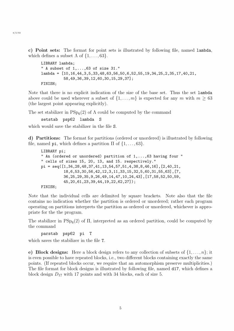
e) Block designs: Here a block design refers to any collection of subsets of 1, . . . , n; itis even possible to have repeated blocks, i.e., two different blocks containing exactly the samepoints. (If repeated blocks occur, we require that an automorphism preserve multiplicities.)The file format for block designs is illustrated by following file, named d17, which defines ablock design D17 with 17 points and with 34 blocks, each of size 5.

5

4/3/92

LIBRARY d17;

" The design with 17 points and 34 blocks, each containing "

" 5 points, obtained from the codewords of weight 5 in the "

" quadratic residue code of length 17 and dimension 9."

d17 = seq( 17, 34,

[3,6,8,15,17], [1,4,7,9,16], [1,4,5,11,17],

[2,5,8,10,17], [3,4,7,8,14], [1,2,5,6,12],

[1,4,6,13,15], [1,3,6,9,11], [1,3,10,12,15],

[3,5,8,11,13], [2,8,9,12,13], [1,7,13,14,17],

[6,8,11,14,16], [4,5,8,9,15], [2,5,7,14,16],

[2,3,6,7,13], [3,4,10,16,17], [3,5,12,14,17],

[1,7,8,11,12], [5,7,10,13,15], [6,12,13,16,17],

[2,4,7,10,12], [2,9,11,14,17], [2,3,9,15,16],

[2,4,11,13,16], [6,7,10,11,17], [4,6,9,12,14],

[5,11,12,15,16], [1,8,10,13,16], [1,2,8,14,15],

[5,6,9,10,16], [4,10,11,14,15], [7,9,12,15,17],

[3,9,10,13,14] );

FINISH;

Note that the file contains the number of points, followed by the number of blocks, followedby a listing of the blocks. Each block is delimited by square brackets.

The automorphism group of this block design could be computed by the command

desauto d17 A

which saves the automorphism group in the file A.

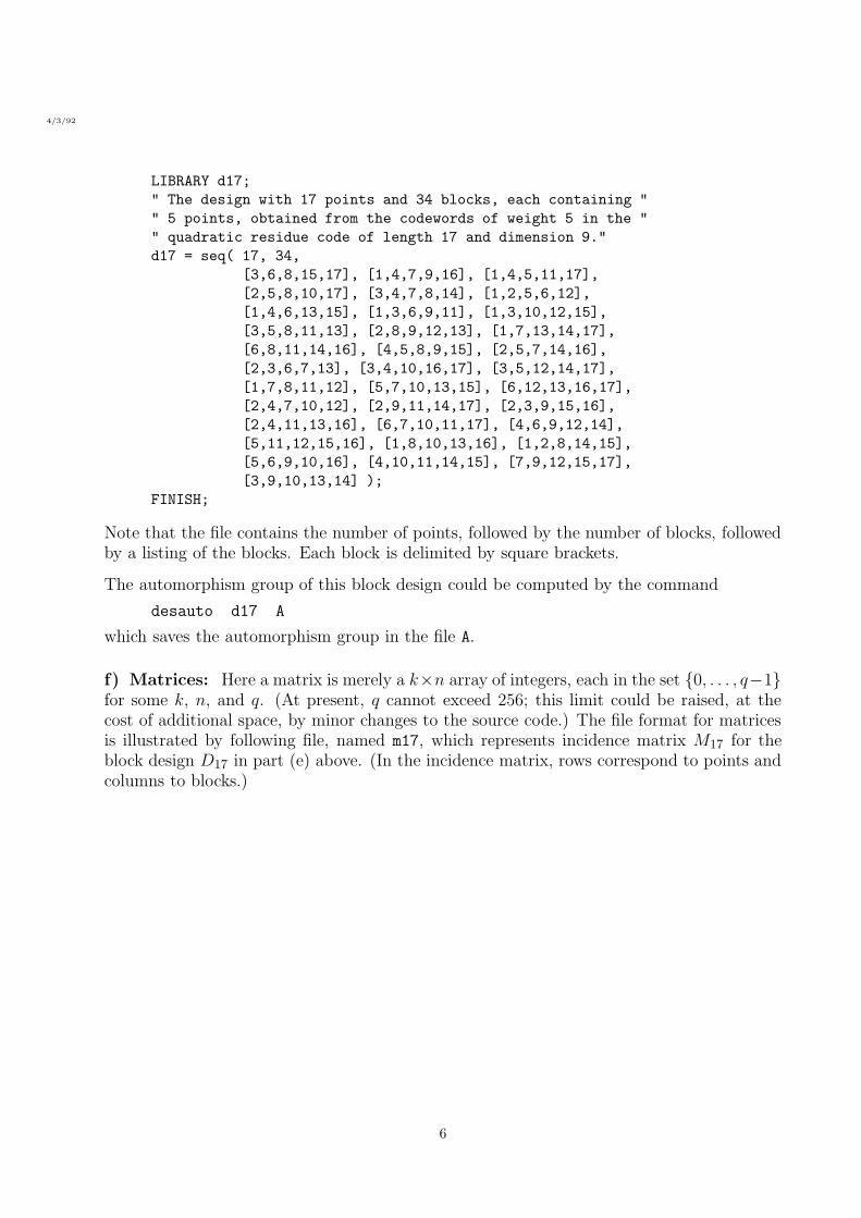
f) Matrices: Here a matrix is merely a k×n array of integers, each in the set 0, . . . , q−1for some k, n, and q. (At present, q cannot exceed 256; this limit could be raised, at thecost of additional space, by minor changes to the source code.) The file format for matricesis illustrated by following file, named m17, which represents incidence matrix M17 for theblock design D17 in part (e) above. (In the incidence matrix, rows correspond to points andcolumns to blocks.)

6

4/3/92

LIBRARY m17;

" The incidence matrix of d17."

m17 = seq( 2, 17, 34, seq(

0,1,1,0,0,1,1,1,1,0,0,1,0,0,0,0,0,0,1,0,0,0,0,0,0,0,0,0,1,1,0,0,0,0,

0,0,0,1,0,1,0,0,0,0,1,0,0,0,1,1,0,0,0,0,0,1,1,1,1,0,0,0,0,1,0,0,0,0,

1,0,0,0,1,0,0,1,1,1,0,0,0,0,0,1,1,1,0,0,0,0,0,1,0,0,0,0,0,0,0,0,0,1,

0,1,1,0,1,0,1,0,0,0,0,0,0,1,0,0,1,0,0,0,0,1,0,0,1,0,1,0,0,0,0,1,0,0,

0,0,1,1,0,1,0,0,0,1,0,0,0,1,1,0,0,1,0,1,0,0,0,0,0,0,0,1,0,0,1,0,0,0,

1,0,0,0,0,1,1,1,0,0,0,0,1,0,0,1,0,0,0,0,1,0,0,0,0,1,1,0,0,0,1,0,0,0,

0,1,0,0,1,0,0,0,0,0,0,1,0,0,1,1,0,0,1,1,0,1,0,0,0,1,0,0,0,0,0,0,1,0,

1,0,0,1,1,0,0,0,0,1,1,0,1,1,0,0,0,0,1,0,0,0,0,0,0,0,0,0,1,1,0,0,0,0,

0,1,0,0,0,0,0,1,0,0,1,0,0,1,0,0,0,0,0,0,0,0,1,1,0,0,1,0,0,0,1,0,1,1,

0,0,0,1,0,0,0,0,1,0,0,0,0,0,0,0,1,0,0,1,0,1,0,0,0,1,0,0,1,0,1,1,0,1,

0,0,1,0,0,0,0,1,0,1,0,0,1,0,0,0,0,0,1,0,0,0,1,0,1,1,0,1,0,0,0,1,0,0,

0,0,0,0,0,1,0,0,1,0,1,0,0,0,0,0,0,1,1,0,1,1,0,0,0,0,1,1,0,0,0,0,1,0,

0,0,0,0,0,0,1,0,0,1,1,1,0,0,0,1,0,0,0,1,1,0,0,0,1,0,0,0,1,0,0,0,0,1,

0,0,0,0,1,0,0,0,0,0,0,1,1,0,1,0,0,1,0,0,0,0,1,0,0,0,1,0,0,1,0,1,0,1,

1,0,0,0,0,0,1,0,1,0,0,0,0,1,0,0,0,0,0,1,0,0,0,1,0,0,0,1,0,1,0,1,1,0,

0,1,0,0,0,0,0,0,0,0,0,0,1,0,1,0,1,0,0,0,1,0,0,1,1,0,0,1,1,0,1,0,0,0,

1,0,1,1,0,0,0,0,0,0,0,1,0,0,0,0,1,1,0,0,1,0,1,0,0,1,0,0,0,0,0,0,1,0

));

FINISH;

Note that the file contains the set size q, followed by the number k of rows, followed by thenumber n of columns, followed by the entries of the matrix listed in row–major order. Notethat matrix entries are not, in general, limited to 0 and 1; if q is the set size, matrix entriesmay be integers in the range 0 through q − 1.

The automorphism group of this matrix could be computed by the command

matauto m17 B

which saves the automorphism group in the file B.

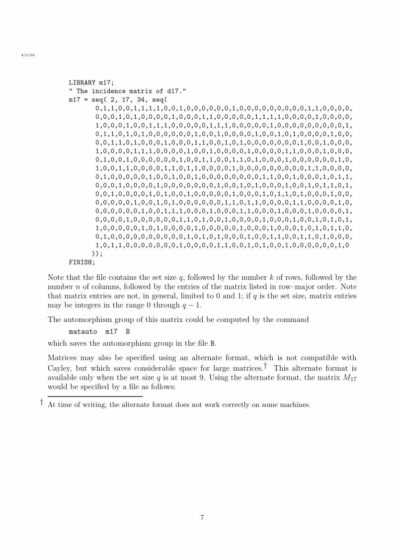
Matrices may also be specified using an alternate format, which is not compatible with

Cayley, but which saves considerable space for large matrices.† This alternate format isavailable only when the set size q is at most 9. Using the alternate format, the matrix M17

would be specified by a file as follows:

† At time of writing, the alternate format does not work correctly on some machines.

7

4/3/92

m17

2 17 34

0110011110010000001000000000110000

0001010000100011000001111000010000

1000100111000001110000010000000001

0110101000000100100001001010000100

0011010001000110010100000001001000

1000011100001001000010000110001000

0100100000010011001101000100000010

1001100001101100001000000000110000

0100000100100100000000110010001011

0001000010000000100101000100101101

0010000101001000001000101101000100

0000010010100000011011000011000010

0000001001110001000110001000100001

0000100000011010010000100010010101

1000001010000100000100010001010110

0100000000001010100010011001101000

1011000000010000110010100100000010

With the alternate format, blanks may occur between matrix entries, but are not required.The first line of the file is reserved for the matrix name; nothing else may be placed on thisline.

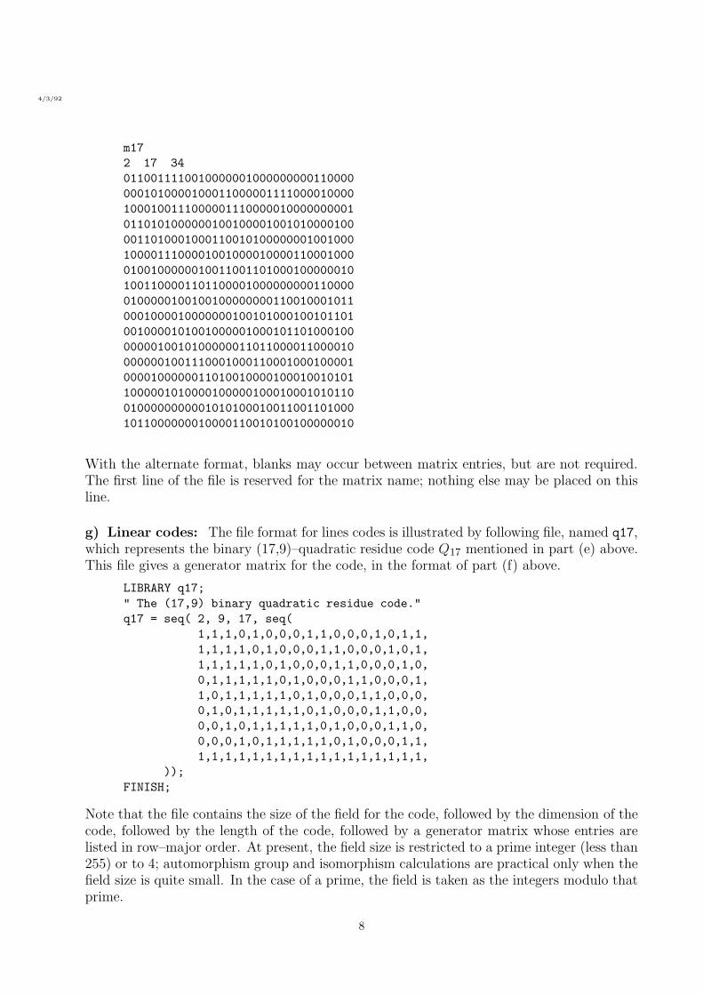
g) Linear codes: The file format for lines codes is illustrated by following file, named q17,which represents the binary (17,9)–quadratic residue code Q17 mentioned in part (e) above.This file gives a generator matrix for the code, in the format of part (f) above.

LIBRARY q17;

" The (17,9) binary quadratic residue code."

q17 = seq( 2, 9, 17, seq(

1,1,1,0,1,0,0,0,1,1,0,0,0,1,0,1,1,

1,1,1,1,0,1,0,0,0,1,1,0,0,0,1,0,1,

1,1,1,1,1,0,1,0,0,0,1,1,0,0,0,1,0,

0,1,1,1,1,1,0,1,0,0,0,1,1,0,0,0,1,

1,0,1,1,1,1,1,0,1,0,0,0,1,1,0,0,0,

0,1,0,1,1,1,1,1,0,1,0,0,0,1,1,0,0,

0,0,1,0,1,1,1,1,1,0,1,0,0,0,1,1,0,

0,0,0,1,0,1,1,1,1,1,0,1,0,0,0,1,1,

1,1,1,1,1,1,1,1,1,1,1,1,1,1,1,1,1,

));

FINISH;

Note that the file contains the size of the field for the code, followed by the dimension of thecode, followed by the length of the code, followed by a generator matrix whose entries arelisted in row–major order. At present, the field size is restricted to a prime integer (less than255) or to 4; automorphism group and isomorphism calculations are practical only when thefield size is quite small. In the case of a prime, the field is taken as the integers modulo thatprime.

8

4/3/92

The automorphism group of this code could be computed by the command

codeauto q17 v17 H

which saves the automorphism group as the group H. (Here file v17 defines a matrix V17

which is the transpose of the matrix M17 of part (f) above; the role of V17 will be explainedlater.)

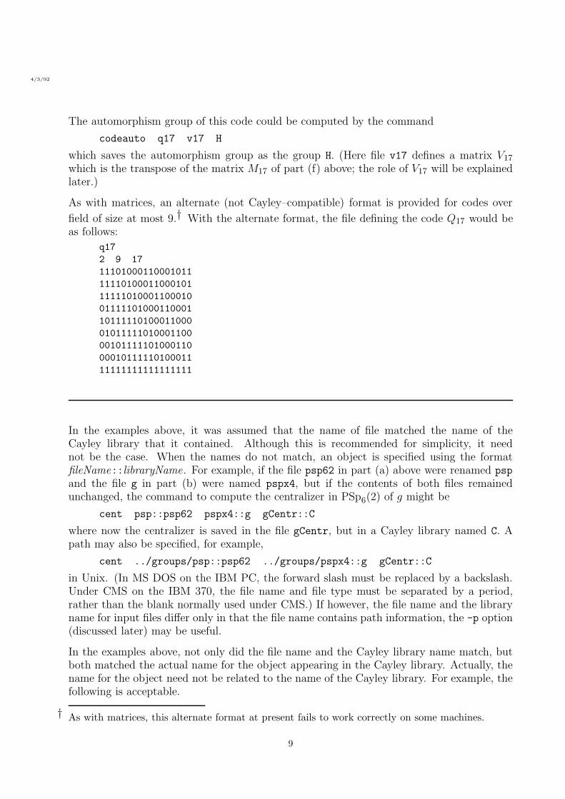
As with matrices, an alternate (not Cayley–compatible) format is provided for codes over

field of size at most 9.† With the alternate format, the file defining the code Q17 would beas follows:

q17

2 9 17

11101000110001011

11110100011000101

11111010001100010

01111101000110001

10111110100011000

01011111010001100

00101111101000110

00010111110100011

11111111111111111

In the examples above, it was assumed that the name of file matched the name of theCayley library that it contained. Although this is recommended for simplicity, it neednot be the case. When the names do not match, an object is specified using the formatfileName::libraryName. For example, if the file psp62 in part (a) above were renamed psp

and the file g in part (b) were named pspx4, but if the contents of both files remainedunchanged, the command to compute the centralizer in PSp6(2) of g might be

cent psp::psp62 pspx4::g gCentr::C

where now the centralizer is saved in the file gCentr, but in a Cayley library named C. Apath may also be specified, for example,

cent ../groups/psp::psp62 ../groups/pspx4::g gCentr::C

in Unix. (In MS DOS on the IBM PC, the forward slash must be replaced by a backslash.Under CMS on the IBM 370, the file name and file type must be separated by a period,rather than the blank normally used under CMS.) If however, the file name and the libraryname for input files differ only in that the file name contains path information, the -p option(discussed later) may be useful.

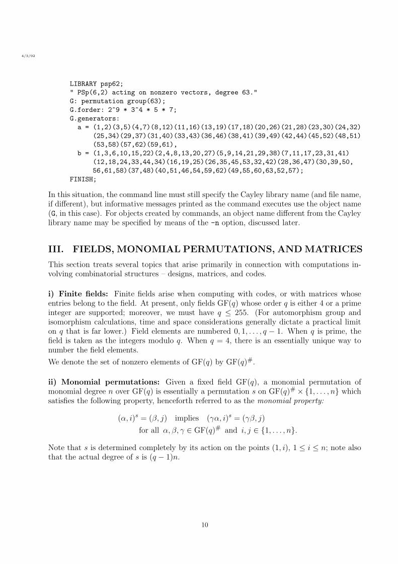
In the examples above, not only did the file name and the Cayley library name match, butboth matched the actual name for the object appearing in the Cayley library. Actually, thename for the object need not be related to the name of the Cayley library. For example, thefollowing is acceptable.

† As with matrices, this alternate format at present fails to work correctly on some machines.

9

4/3/92

LIBRARY psp62;

" PSp(6,2) acting on nonzero vectors, degree 63."

G: permutation group(63);

G.forder: 2^9 * 3^4 * 5 * 7;

G.generators:

a = (1,2)(3,5)(4,7)(8,12)(11,16)(13,19)(17,18)(20,26)(21,28)(23,30)(24,32)

(25,34)(29,37)(31,40)(33,43)(36,46)(38,41)(39,49)(42,44)(45,52)(48,51)

(53,58)(57,62)(59,61),

b = (1,3,6,10,15,22)(2,4,8,13,20,27)(5,9,14,21,29,38)(7,11,17,23,31,41)

(12,18,24,33,44,34)(16,19,25)(26,35,45,53,32,42)(28,36,47)(30,39,50,

56,61,58)(37,48)(40,51,46,54,59,62)(49,55,60,63,52,57);

FINISH;

In this situation, the command line must still specify the Cayley library name (and file name,if different), but informative messages printed as the command executes use the object name(G, in this case). For objects created by commands, an object name different from the Cayleylibrary name may be specified by means of the -n option, discussed later.

III. FIELDS, MONOMIAL PERMUTATIONS, AND MATRICES

This section treats several topics that arise primarily in connection with computations in-volving combinatorial structures – designs, matrices, and codes.

i) Finite fields: Finite fields arise when computing with codes, or with matrices whoseentries belong to the field. At present, only fields GF(q) whose order q is either 4 or a primeinteger are supported; moreover, we must have q ≤ 255. (For automorphism group andisomorphism calculations, time and space considerations generally dictate a practical limiton q that is far lower.) Field elements are numbered 0, 1, . . . , q − 1. When q is prime, thefield is taken as the integers modulo q. When q = 4, there is an essentially unique way tonumber the field elements.

We denote the set of nonzero elements of GF(q) by GF(q)#.

ii) Monomial permutations: Given a fixed field GF(q), a monomial permutation ofmonomial degree n over GF(q) is essentially a permutation s on GF(q)#×1, . . . , n whichsatisfies the following property, henceforth referred to as the monomial property:

(α, i)s = (β, j) implies (γα, i)s = (γβ, j)

for all α, β, γ ∈ GF(q)# and i, j ∈ 1, . . . , n.

Note that s is determined completely by its action on the points (1, i), 1 ≤ i ≤ n; note alsothat the actual degree of s is (q − 1)n.

10

4/3/92

For purposes of actual computation, however, we want a representation of s as a permutationon 1, . . . , (q − 1)n; to obtain this, we number the pair (α, i) by (q − 1)(i− 1) + α, whereα denotes the integer representing α. Then the monomial property becomes

((q − 1)(i− 1) + α)s = (q − 1)(j − 1) + β implies

((q − 1)(i− 1) + γα)s = (q − 1)(j − 1) + γβ.

For example, over the field GF(4), the monomial permutation s on GF(4) × 1, 2, 3, 4determined by

(1, 1)s = (3, 2), (1, 2)s = (2, 4), (1, 3)s = (1, 1), (1, 4)s = (2, 3)

is represented as a permutation on 1, . . . , 12 as follows:

(1, 6, 10, 8, 2, 4, 11, 9, 3, 5, 12, 7).

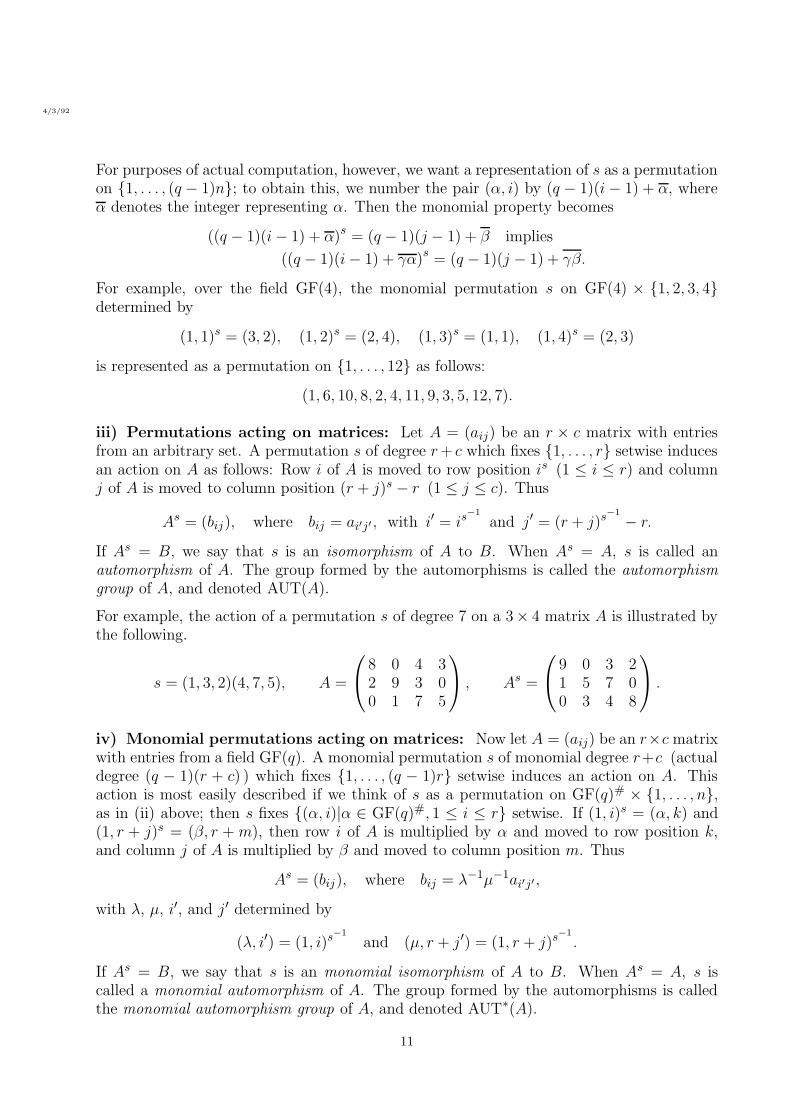
iii) Permutations acting on matrices: Let A = (aij) be an r × c matrix with entriesfrom an arbitrary set. A permutation s of degree r+ c which fixes 1, . . . , r setwise inducesan action on A as follows: Row i of A is moved to row position is (1 ≤ i ≤ r) and columnj of A is moved to column position (r + j)s − r (1 ≤ j ≤ c). Thus

As = (bij), where bij = ai′j′ , with i′ = is−1

and j′ = (r + j)s−1 − r.

If As = B, we say that s is an isomorphism of A to B. When As = A, s is called anautomorphism of A. The group formed by the automorphisms is called the automorphismgroup of A, and denoted AUT(A).

For example, the action of a permutation s of degree 7 on a 3× 4 matrix A is illustrated bythe following.

s = (1, 3, 2)(4, 7, 5), A =

8 0 4 32 9 3 00 1 7 5

, As =

9 0 3 21 5 7 00 3 4 8

.

iv) Monomial permutations acting on matrices: Now let A = (aij) be an r×c matrixwith entries from a field GF(q). A monomial permutation s of monomial degree r+c (actualdegree (q − 1)(r + c) ) which fixes 1, . . . , (q − 1)r setwise induces an action on A. Thisaction is most easily described if we think of s as a permutation on GF(q)# × 1, . . . , n,as in (ii) above; then s fixes (α, i)|α ∈ GF(q)#, 1 ≤ i ≤ r setwise. If (1, i)s = (α, k) and(1, r + j)s = (β, r + m), then row i of A is multiplied by α and moved to row position k,and column j of A is multiplied by β and moved to column position m. Thus

As = (bij), where bij = λ−1µ−1ai′j′ ,

with λ, µ, i′, and j′ determined by

(λ, i′) = (1, i)s−1

and (µ, r + j ′) = (1, r + j)s−1

.

If As = B, we say that s is an monomial isomorphism of A to B. When As = A, s iscalled a monomial automorphism of A. The group formed by the automorphisms is calledthe monomial automorphism group of A, and denoted AUT∗(A).

11

4/3/92

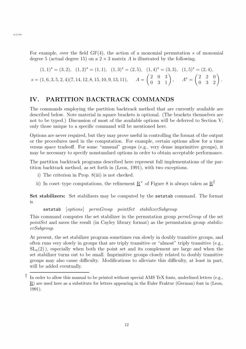
For example, over the field GF(4), the action of a monomial permutation s of monomialdegree 5 (actual degree 15) on a 2× 3 matrix A is illustrated by the following.

(1, 1)s = (3, 2), (1, 2)s = (1, 1), (1, 3)s = (2, 5), (1, 4)s = (3, 3), (1, 5)s = (2, 4),

s = (1, 6, 3, 5, 2, 4)(7, 14, 12, 8, 15, 10, 9, 13, 11), A =

(2 0 30 3 1

), As =

(2 2 00 3 2

).

IV. PARTITION BACKTRACK COMMANDS

The commands employing the partition backtrack method that are currently available aredescribed below. Note material in square brackets is optional. (The brackets themselves arenot to be typed.) Discussion of most of the available options will be deferred to Section V;only those unique to a specific command will be mentioned here.

Options are never required, but they may prove useful in controlling the format of the outputor the procedures used in the computation. For example, certain options allow for a timeversus space tradeoff. For some “unusual” groups (e.g., very dense imprimitive groups), itmay be necessary to specify nonstandard options in order to obtain acceptable performance.

The partition backtrack programs described here represent full implementations of the par-tition backtrack method, as set forth in (Leon, 1991), with two exceptions.

i) The criterion in Prop. 8(iii) is not checked.

ii) In coset–type computations, the refinement R+ of Figure 8 is always taken as R†

Set stabilizers: Set stabilizers may be computed by the setstab command. The formatis

setstab [options] permGroup pointSet stabilizerSubgroup

This command computes the set stabilizer in the permutation group permGroup of the setpointSet and saves the result (in Cayley library format) as the permutation group stabiliz-erSubgroup.

At present, the set stabilizer program sometimes run slowly in doubly transitive groups, andoften runs very slowly in groups that are triply transitive or “almost” triply transitive (e.g.,SLn(2) ), especially when both the point set and its complement are large and when theset stabilizer turns out to be small. Imprimitive groups closely related to doubly transitivegroups may also cause difficulty. Modifications to alleviate this difficulty, at least in part,will be added eventually.

† In order to allow this manual to be printed without special AMS TeX fonts, underlined letters (e.g.,

R) are used here as a substitute for letters appearing in the Euler Fraktur (German) font in (Leon,

1991).

12

4/3/92

Set images: Given a permutation group G on 1, . . . , n and subsets Λ and Φ of 1, . . . , n,the setimage command may be used to determine if there exists an element g of G suchthat Λg = Φ. The format is

setimage [options] permGroup pointSet1 pointSet2 groupElement

where permGroup, pointSet1, pointSet2, and groupElement play the role of G, Λ, Φ, andg, respectively. That is, the command determines whether there exists an element of per-mGroup mapping pointSet1 to pointSet2 and, if so, saves one such element as the permu-tation groupElement. Note that groupElement will not be created if Φ /∈ ΛG. (Unless the-q option is specified, a message indicating whether Φ ∈ ΛG will be written to the standardoutput.) The potential difficulties with doubly and triply transitive groups mentioned forset stabilizer computations apply here also.

Ordered partition stabilizers: Stabilizers of ordered partitions may be computed by theparstab command. The format is

parstab [options] permGroup ordPartition stabilizerSubgroup

This command computes the stabilizer in the permutation group permGroup of the orderedpartition ordPartition and saves the result as the permutation group stabilizerSubgroup.The remarks about performance on doubly and triply transitive groups for set stabilizercomputations apply here also.

Ordered partition images: Given a permutation group G on 1, . . . , n and orderedpartitions Π and Σ of 1, . . . , n, the parimage command may be used to determine if thereexists an element g of G such that Πg = Σ. The format is

parimage [options] permGroup ordPartition1 ordPartition2 groupElement

where permGroup, ordPartition1, ordPartition2, and groupElement play the role of G, Π, Σ,and g, respectively. That is, the command determines whether there exists an element ofpermGroup mapping ordPartition1 to ordPartition2 and, if so, saves one such element asthe permutation groupElement. The permutation groupElement is created only if Σ ∈ ΠG.The remarks about performance on doubly and triply transitive groups given above for setstabilizer computations apply here also.

Group intersections: Given permutation groups G and H on 1, . . . , n, the inter com-mand may be used compute the intersection G ∩H. The format is

inter [options] permGroup1 permGroup2 interGroup

This command computes the intersection of groups permGroup1 and permGroup2 and savesthe result as the group interGroup. The potential difficulty with doubly and triply transitivegroups discussed above for set stabilizer computations applies here also when both groupsare doubly or triply transitive.

13

4/3/92

Centralizers of elements: Given a permutation group G and a permutation x (not nec-essarily contained in G), the cent command may be used compute CG(x), the centralizer inG of x. The format is

cent [options] permGroup permutation centralizerSubgroup

Here permGroup, permutation, and centralizerSubgroup play the role of G, x, and CG(x)above. That is, the command computes the centralizer in the group permGroup of thepermutation permutation and saves the result as the group centralizerSubgroup.

For this command, it is permissible to specify permGroup as #n, where n is an integer at least2, in which case permGroup is taken as the symmetric group of degree n; in this situation,the normal restrictions on base size (discussed later) do not apply to permGroup, althoughthey do apply to centralizerSubgroup.

The cent command accepts an option -np which can have an effect (often small) on perfor-mance. If this option is specified, a refinement process based on the cycle structure of x willnot be used. The effect is to reduce memory requirements a bit. In many cases, the runningtime does not change significantly, but in some cases it does increase a great deal.

It should be noted that in many cases, perhaps most cases arising in practice, centralizercomputations are fairly easy even for conventional algorithms, and the partition backtrackprogram may perform no better than, and perhaps not even as well as, programs based onconventional techniques, such as those in Cayley. (Note, however, that, unlike Cayley, theprogram here does not require that the permutation to be centralized lie in the group.)

Conjugacy of elements: Given a permutation group G and permutations x and y (notnecessarily contained in G), the conj command may be used to determine if x and y areconjugate under G and, if so, to find g in G with xg = y. The format is

conj [options] permGroup permutation1 permutation2 conjugatingElement

Here permGroup, permutation1, permutation2, and conjugatingElement play the role of G,x, y, and g above. That is, the command determines if there exists an element of permGroupconjugating permutation1 to permutation2 and, if so, it saves one such element as the per-mutation conjugatingElement. If the two permutations are not conjugate in permGroup, thenconjugatingElement is not created. In any case, a message indicating the result is written tothe standard output (unless the -q option is specified).

As with the cent command, permGroup may be specified as #n, in which case conjugacy inthe symmetric group of degree n is checked. (In this case, the program merely checks thatthe two permutations have the same cycle structure.) Also, the -np option is accepted, andit works as described above for the cent command.

As with centralizer computations, conjugacy calculations are usually easy with conventionalalgorithms, and the partition backtrack method may not yield an improvement.

14

4/3/92

Centralizers of groups: Given a permutation groups G and a second permutation groupE (not necessarily contained in G), the gcent command may be used compute CG(E), thecentralizer in G of E. The format is

gcent [options] permGroup1 permGroup2 centralizerSubgroup

Here permGroup1, permGroup2, and centralizerSubgroup play the role of G, E, and CG(E)above. That is, the command computes the centralizer in the group permGroup1 of thegroup permGroup2 and saves the result as the group centralizerSubgroup.

As with the element centralizer command (cent), it is permissible to specify permGroup1as #n, indicating the symmetric group of degree n.

To an even greater extent than element centralizer calculations, group centralizer calcula-tions tend to be easy ones for conventional algorithms; the full power of the partition methodis not needed, and perhaps not even desirable. For this reason, little effort has gone intodevelopment of the gcent command; its implementation is fairly crude, and it is includedprimarily for completeness. There are two options, -cg:m and -cp:p, which affect its per-formance; for some groups G, it may be necessary to assign them values different from thedefaults (current 3 and 10, respectively). A full description of the significance of m and p willnot be given here; however, we note that higher values (especially for m) increase memoryrequirements, and often increase execution time as well, but may be needed if the group Efails to have a small generating set (e.g., if E is a large elementary abelian group).

By specifying permGroup1 and permGroup2 as the same group, the gcent command maybe used to compute the center of a group; note, however, that it represents an exceptionallyinefficient algorithm for this purpose.

Automorphism groups of designs: The desauto command may be used to computethe automorphism group of a design. Here a design means any set of points (numbered1, . . . , n for some n) and any collection of subsets of the point set. The format of the designautomorphism group command is:

desauto [options] design autoGroup

and the command sets autoGroup to the automorphism group of the design design.

The interpretation of the group autoGroup that is created depends on whether the -pb

(points and blocks) option is specified. Let p and b denote the number of points and blocks,respectively, of the design.

i) If the option -pb is specified, then autoGroup is constructed as a group of degreep+b, in which the action on 1, . . . , p is the action on points and in which the actionon p+1, . . . , p+ b is the action on blocks, the j th block being represented by p+ j.

ii) If the -pb option is omitted, then autoGroup is constructed as a group of degree p,representing the action on points only. In this case, if there are repeated blocks, thegroup acting on points only has lower order than the group acting on points andblocks). When this situation arises, the group saved as autoGroup represents thegroup on points only, but the information written to the standard output duringthe computation refers to the group acting on points and blocks. (This occursbecause the computation is carried out on points and blocks; restriction to points

15

4/3/92

is performed only at the end; note also, for this reason, restriction to points onlydoes not save time or memory.)

Isomorphism of designs: The desiso command may be used to check isomorphism ofdesigns. The format is

desiso [options] design1 design2 isoPerm

and the command sets isoPerm to an isomorphism from design design1 to design design2,provided the designs are isomorphic. (If not, the permutation isoPerm is not created. Inany case, a message indicating the result is written to the standard output, unless the -q

option is specified.)

As in the case of the desauto command, described above, the presence or absence of the -pb

option determines whether isoPerm is constructed as a permutation on points and blocks,or on points only (the default). When the action on blocks is included, the j th block isrepresented by p+ j.

Automorphism groups and monomial groups of matrices: The matauto commandmay be used to compute the automorphism group of a matrix. If the matrix elements aretaken from a small finite field GF(q), then optionally the monomial automorphism groupmay be computed. (See Section III for definitions.) The command format is:

matauto [options] matrix autoGroup

and the command sets autoGroup to the automorphism group of the matrix matrix or, ifthe -mm option is specified, to the monomial automorphism group of matrix .

If the -tr option is specified, the matrix is transposed after it is read in, and all computationsapply to the transposed matrix.

Let r and c denote the number of rows and columns, respectively, of the matrix A = (aij)whose group is to be constructed. Normally the automorphism group has degree r + c andthe monomial automorphism group has degree (q − 1)(r + c); the interpretation of thesegroups is described in Section III. However, if the -ro (rows only) option is specified, thedegree will be r or (q− 1)r, and the group will represent the action on rows only. Note thatrestriction to rows only may reduce the order of the group, just as in the case of designsrestriction to points only may reduce the order of the group. When this occurs, the remarksabove for design groups apply here also.

At present, the program for computing monomial groups of matrices is a very crude one. Asa result, although it works reasonably for many matrices of fairly large size, it can fail torun in acceptable time even for very small matrices, e.g., matrices of all 0s. Sometimes useof the -tr option can get around this difficulty (which will be fixed eventually).

16

4/3/92

Isomorphism and monomial isomorphism of matrices: The matiso command maybe used to check if two matrices are isomorphic or, if the matrix elements are from a finitefield GF(q), monomially isomorphic. (See Section III for definitions.) The command formatis

matiso [options] matrix1 matrix2 isoPerm

In the absence of the -mm option, the command sets isoPerm to an isomorphism from matrixmatrix1 to matrix matrix2, provided the matrices are isomorphic. (If not, the permutationisoPerm is not created). If the -mm option is specified, the command sets isoPerm to amonomial isomorphism from matrix matrix1 to matrix matrix2, provided the matrices aremonomially isomorphic. (In this case, the matrix entries should be field elements.) Theeffect of the -ro option is as described above for matrix automorphism group calculations.

Currently the monomial isomorphism program suffers from the same limitations as the mono-mial automorphism group program, as mentioned above.

Automorphism groups of linear codes: The codeauto command may be used to com-pute the automorphism group of a linear code over a small field GF(q). However, before theautomorphism group of a code C may be computed, it is necessary to have a set V of vectors(not necessarily codewords) such that the following conditions hold. In these conditions, V ∗

denotes the set of all nonzero scalar multiples of vectors in V .

i) No vector in V is a scalar multiple of any other vector in V . (In particular, |V ∗| =(q − 1)|V |.)

ii) V is “reasonably small”. (With a very large memory, “reasonably small” might mean100,000 or more.)

iii) V ∗ is invariant under AUT(C) (the automorphism group of C),

iv) |AUT(V ∗) : AUT(C)| is very small. (The running time rises very rapidly as a functionof this index. Note that, if V spans C, the index is 1.)

Often the set of minimal weight vectors of the code (scalar multiples removed if q > 2)make a suitable choice for V ; minimum weight vectors of the dual code may also be used.This choice for V certainly satisfies (i) and (iii), may well satisfy (ii), and in many casessatisfies (iv). The author has available programs for computing the set of minimum weightvectors (or vectors of any specified weight.)

The format of the code automorphism group command is

codeauto [options] code invarVectors autoGroup

where invarVectors is the set V of vectors described above (in the format of a matrix, whoserows are the vectors). The command sets autoGroup to the automorphism group of the codecode.

17

4/3/92

The -cv (coordinates and vectors) option for codes has essentially the same effect as the-pb option for designs. With this option, the automorphism group is saved in autoGroupas a permutation group of degree (q − 1)(n + |V |) (n = length of code), representing theaction on (monomial) coordinates and invariant vectors; without the -cv option, it is savedas a permutation group acting of degree (q − 1)n, representing the action on (monomial)coordinates only. (However, restriction to coordinates only can never lead to a reduction inthe group order, as occurred with restriction to points or rows for designs or matrices.) Foran explanation of the format of monomial permutations, see Section III.

At present, the program for computing groups of non–binary codes is a very crude one;sometimes it can fail to run in reasonable time even on small codes. Eventually this programwill be improved.

Isomorphism of linear codes: The codeiso command may be used to check isomorphismof linear codes. However, before isomorphism of two codes C1 and C2 may be checked, it isnecessary to have a sets V1 and V2 of vectors (not necessarily codewords of the two codes)such that V1 and V2 satisfy conditions (i), (ii), (iii), and (iv) above relative to C1 and C2,respectively, and in addition such that any isomorphism of C1 to C2 must map V ∗1 to V ∗2 .(As with code automorphism groups, V ∗1 and V ∗2 denote the sets of nonzero scalar multiplesof vectors in V1 and V2, respectively. Often suitable choices for V1 and V2 are the minimalweight vectors of C1 and C2, respectively (scalar multiples removed.); minimal weight vectorsof the duals of the two codes also could be used.

The format of the code isomorphism command is

codeiso [options] code1 code2 invarVectors1 invarVectors2 isoPerm

where invarVectors1 and invarVectors2 are the sets V1 and V2, respectively, of vectors de-scribed above (each in the format of a matrix, whose rows are the vectors). The commandsets isoPerm to an isomorphism from code1 to code2, if the codes are isomorphic; if not,isoPerm is not created.

As in the case of the codeauto command, described above, the presence or absence ofthe -cv option determines whether isoPerm is a permutation on (monomial) coordinatesand invariant vectors, or on (monomial) coordinates only. The interpretation of monomialpermutations is described in Section III..

Note that a number of the commands above are implemented as shell files (under Unix), batchfiles (under MS DOS), or exec files (under CMS). The commands that are implemented inthis manner, and the contents of the Unix shell files, are as follows. (The list includes a fewcommands to be discussed in Section IX.)

18

4/3/92

command contents of shell file

setimage setstab -image $*

parstab setstab -partn $*

parimage setstab -image -partn $*

conj cent -conj $*

gcent cent -group $*

desiso desauto -iso $*

matauto desauto -matrix $*

matiso desauto -iso -matrix $*

codeauto desauto -code $*

codeiso desauto -iso -code $*

cjper cjrndper -perm $*

ncl commut -ncl $*

compper compgrp -perm:$1 $2 $3

compset compgrp -set:$1 $2 $3

chbase orblist -chbase $*

ptstab orblist -ptstab $*

V. OPTIONS

A partial description of the options that are currently available follows. Most of the optionsare available with all of the commands described in Section IV. A few options apply only tosubgroup computations, or only to coset–representative computations; these restrictions arenoted below. Options applicable only to a single command are discussed with that commandin Section IV.

In general, options may be specified in any order. However, if conflicting options are specified,the one specified last is the one that is used. (In some cases, conflicting options are treatedas an error. Also, the -l and -v options, discussed later, are an exception to the generalrule that options may be specified in any order; these options, if present, must come first,and the remainder of the command line is ignored.)

Entering any command with no options or arguments causes a brief summary of the commandformat to be displayed.

Options affecting file handling:

-a Normally, if a file name is specified for an object to be constructed, andif a file by that name already exists, the programs overwrite the existingfile. With the -a option, they append to the existing file, rather thanoverwriting it.

19

4/3/92

-p:path Here path is a string. The string path is concatenated to the file nameof every input file. This option can be useful if all the input files are inanother directory. For example,

setstab ../groups/psp62::psp62 ../groups/lambda::lambda S

may be written more compactly as

setstab -p:../groups/ psp62 lambda S

(Note the final slash following groups is required.). The -p option has noeffect on output files.

Options affecting output format:

-i This option applies to commands that construct and write out either apermutation or a permutation group. It causes permutations to be writtenin image format, rather than in cycle format (the default).

-n:name Here name is a string. The object created by the command will be namedname. By default, the name assigned to the object will be the name of theCayley library containing its definition. Note this option affects only thename of the object, not that of the file or the Cayley library.

-q Suppresses informative messages on the state of the computation, normallywritten to the standard output during the computation.

-s Causes statistics on the pruning of the backtrack search tree to be writ-ten out to the standard output. These statistics relate to the backtracksearch tree defined in the author’s paper (Leon, 1991), and are likely to bemeaningful only to users familiar with that paper.

-w:n Here n should be a nonnegative integer. This option applies only to cosetrepresentative computations. If the degree is less than or equal to n, and if acoset representative is found, it will be included in the informative messageswritten to the standard output. (In any case, the coset representative willbe written to a file in Cayley library format.) The default value of n iscurrently 300.

Options affecting performance of the algorithm:

-b:k Here k is a nonnegative integer which determines the extent to which basechanges are performed in an attempt to improve pruning of the backtracksearch tree using tests on double–coset minimality (Leon, 1991, Prop 8).When k = 0, base change is never performed (except during R–base con-struction, when it is used for a different purpose). As k increases, thenumber of base change operations performed increases; however, increas-ing k beyond the base size produces no further increase in the number ofbase change operations. Designating k = 0 reduces memory requirementsand often produces the best running times as well. On the other hand,some high–density groups seem to require a higher value of k in order to

20

4/3/92

obtain acceptable performance. By default, the program chooses a valueof k based on the density and degree of transitivity of the group; quiteoften, this default value is 0.

Note: For coset representative computations, this option has no effect un-less known subgroups of the two associated groups are specified; see dis-cussion of the -kL and -kR options below.

-g:m Here m should be a nonnegative integer. This is one of several parametersproviding a time vs. space tradeoff. Small values of m, say 10 or less,minimize memory requirements, while large values of m, say 100 or greater,reduce the running time moderately for most difficult groups. Use of a highvalue is recommended for multiply transitive groups.

After R–base construction, the program attempts to reduce the height ofthe Schreier trees for the containing group by adding new strong generators.However, it will never add generators for this purpose if doing so wouldcause the total number of strong generators to exceed m. (It will also stopadding generators if the height falls below certain goals currently fixed inthe program.)

-k:H Here H specifies a permutation group (in the format cayleyLibraryNameor fileName::cayleyLibraryName). This option applies only to subgroupcalculations. The group H must be a known subgroup of the group beingcomputed. In principle, this option allows one to take advantage of anysubgroup of the group being computed that happens to be known in ad-vance. In practice, however, it seldom appears to speed up the computationby very much, and it increases memory requirements.

-kL:J

-kR:M

Here J and M must specify permutation groups (each in the format cay-leyLibraryName or fileName::cayleyLibraryName). These options applyonly to coset representative calculations. Either or both may be speci-fied. Associated with every coset representative computation, there are“left” and “right” groups, as explained in Section 2 of (Leon, 1991).The groups J and M must be known subgroups of these left and rightgroups, respectively. Specifying J and/or M , if known, increases mem-ory requirements, but in some cases it may improve the running time.For some very dense groups, one or both of these options may be neededin order to allow the computation to finish in an acceptable amount oftime.

-mb:k Here k should be a nonnegative integer. This integer represents an upperbound on the size of the base for a permutation group. The default valueof k is 62, which is more than adequate for many groups. For furtherdiscussion of the -mb option, see Section VII.

-mw:` Here ` should be a nonnegative integer whose value is at least severalhundred. This integer represents an upper bound on the length of anyword in the generators of any permutation group. For further discussion,see Section VII.

21

4/3/92

-r:p Here p should be a nonnegative integer, normally smaller than the integerm specified for the -g option described above. This is another optionproviding for a time versus space tradeoff. Small values of p, say less than10, minimize memory requirements, while larger values, say 50 or higher,may reducing the running time, although usually not a great deal.

Whenever the number of strong generators for the containing group exceedsp, redundant strong generators are eliminated, using a procedure originallydue to Sims (1971).

Special options:

-l This option, if present, must be the first option on the command line,and the remainder of the command line is ignored. (It may be omitted.)The -l option merely prints out limits on the default maximum base size,default maximum word length, degree, and other quantities with which thisversion of the program has been compiled. (See Section VII for discussionof these limits.)

-v This option, if present, must be the first option on the command line, andthe remainder of the command line is ignored. (It may be omitted.) The-v option is intended to be used once following compilation of the program.It attempts to check that all the source files for the program were compiledwith the same options and size limits. (See Section VII for discussion ofsize limits.)

VI. OUTPUT AND RETURN CODES

All programs for subgroup computations return a value of 0 if the computation is completedsuccessfully and a nonzero value (currently 15) if the computation terminates due to an error(input file not found, incorrect format in input file, memory exhausted, size limit in programexceeded, etc.) All programs for coset representative computations return a value of 0 if thecomputation is completed successfully and a coset representative exists, 1 if it is completedbut a coset representative does not exist, and a value different from 0 and 1 (currently 15)if the computation terminates due to an error.

Unless the -q option is specified, all of the programs write information about the progressof the computation to the standard output. Some of this information, most notably thatrelating to the R–base and the backtrack search tree (the latter given only if -s is specified)will probably be meaningful primarily to users familiar with the author’s paper (Leon, 1991).Information of more general interest includes:

i) The order of the containing group (unless it is the symmetric group). Note that thisorder is determined by computing a base and strong generating set for the containinggroup when it is read in, unless they are supplied in the input file.

ii) The new (changed) base and strong generating set for the containing group computedduring R–base construction, and the corresponding basic orbit lengths. In the notationof (Leon, 1991), this is the base (α1, . . . , αk) associated with the R–base.

22

4/3/92

iii) A base for the subgroup to be computed (subgroup computations) or for the subgroupassociated with the right coset whose representative is to be computed (coset repre-sentative computations). This is the subgroup base associated with the R–base; inthe notation of (Leon, 1991), it is (α1, . . . , α`). Note that this base is a subsequenceof the base for the containing group in (ii) above.

iv) The basic cell sizes corresponding to the subgroup base in (iii) above (for definitions,see (Leon, 1991)). Note that each basic cell size provides an upper bound for thecorresponding basic orbit length of the subgroup to be computed (subgroup–typecomputations). (Usually the bound is not sharp).

v) The number of strong generators for the containing group and the mean node depthsin the Schreier trees for the basic orbits of the containing group. Depending on the -g

and -r options, following R–base construction, additional strong generators may beadded in an attempt to reduce the height of the Schreier trees. Figures are providedboth before and after additional strong generators are added.

vi) [subgroup computations only] A message for each strong generator that is found forthe subgroup. The message gives the level and the basic orbit lengths for the subgroupconstructed thus far. (A generator will be said to be at level i if it fixes the first i− 1base points but moves the ith.)

vii) [subgroup computations only] The order of the subgroup that was computed.

viii) [subgroup computations only] The base (same as in (iii) above) and basic orbit lengthsfor the subgroup that was computed.

ix) [coset representative computations only] A message indicating whether a coset repre-sentative exists.

x) [coset representative computations only] If a coset representative exists and the degreeis sufficiently low (depending on the -w option), the coset representative that wasfound.

xi) The time required for the computation. Note that the time to read in the containinggroup from a file, construct the initial base and strong generating set for the containinggroup (if not present in the input file), and to write out the subgroup or coset represen-tative to a file is not included in this time. All computations relating to calculation ofthe subgroup or coset representative (including base changes in the containing group)are included.

Note that, in subgroup computations, the actual strong generators for the subgroup arenot written to standard output, and in coset computations, the actual coset representativefound may not (depending on the degree and -w option) be written to the standard output.However, both may be found (in Cayley library format) in the output file that is created.

For design, matrix, or code isomorphism computations, the isomorphism that is constructedis written to the standard output (assuming that the degree is sufficiently low) in a moreeasily readable (but not Cayley compatible) format than that described in Sections II and III.For designs with the -pb option, the action on points and blocks is given separately. For

23

4/3/92

matrices, the action on rows and columns is given separately. For monomial isomorphism ofmatrices for non–binary codes, the monomial isomorphism is written in the following format:

([λ1]i1, [λ2]i2, . . . , [λk]ik )

This denotes the monomial permutation mapping 1 to λ1i1, 2 to λ2i2, etc. For example, toapply this monomial permutation to the rows of an r by c matrix, row j is multiplied by λjand the result is moved to row position ij .

VII. SIZE LIMITS

There are a few fixed limits on the sizes of objects that the programs can handle. Theselimits can be changed only by recompiling the programs. The order of any group may haveat most 30 distinct prime divisors. The name of any file may have at most 60 characters(including path information supplied with the -p option). The name of any object may haveat most 16 characters. Most importantly, if the program is compiled using 16–bit integers,the maximum degree of any permutation group is limited to slightly less than 216 (about65000). If it is compiled using 32–bit integers, there is, for practical purposes, no fixed limit.Note, however, that use of 16–bit integers reduces memory requirements substantially, andit is recommended unless groups of degree greater than 65000 (approx) are to be used. Onlymachines having at least 20 to 25 megabytes of memory are likely to be able to handle groupsof degree high enough to require 32–bit integers. Currently both 16–bit and 32–bit compiledversions of the programs are available.

Although there is no fixed limit on the base size for a permutation group, a limit must beestablished at the time that the program is initiated, and this limit remains fixed duringthat run. This limit may be set at k by means of the -mb:k option, or it may be allowed todefault to 62. Note that large values of k increase running times and memory requirementsslightly even if the actual base size turns out to be much less than k.

For the most part, the amount of memory (real and virtual) available determines the sizes ofobjects that can be handled by the programs. Memory requirements depend heavily on thedegree of the group, and to a somewhat lesser extent on the base size. The programs can usevirtual memory to some extent; however, if virtual memory used exceeds real memory by afactor of more than 1.6 to 1.8, excessive paging is likely to occur. The following steps maybe taken to reduce memory requirements; the steps are listed in order of decreasing benefit.

i) If the degree of the group is less than 65000 (approx), use a 16–bit version of theprogram rather than a 32–bit version. The 16–bit version is likely to run about as fastas the 32–bit version, and it requires a great deal less memory.

ii) Specify options of -g:1 and -r:1. These options are likely to increase the executiontime substantially, but they often save a good deal of memory. As a compromise,values greater than 1 but less than the defaults may be specified, e.g., -g:20 and-r:15

iii) Specify the option -b:0 if it is not already the default. In the majority of cases,this option will not increase execution time, and it reduces memory requirementsconsiderably. However, in a great many cases, -b:0 will already be the default. (The

24

4/3/92

value for this and other options is displayed on the standard output when the programis is run.)

iv) For (element) centralizer and conjugacy calculations, specify the -np option. Thissaves a modest amount of memory. The effect on execution time is hard to predict;in some cases, it may lead to a major increase. For group centralizer calculations,options of -cg:2 and -cp:i, where i is 3 to 5, may be tried, although on some groupsthey may raise the running time to unacceptable levels.

v) Specify the option -mb:k for a value of k less than the default of 62. The -mb:koptions sets a limit of k on the base size for the group; often a value considerably lessthan 62 (e.g., 15 or 20) will be adequate. However, the amount of memory saved isrelatively small.

In the author’s experience, the programs can often handle groups of degree as high as 2000mto 3000m, where m is the number of megabytes of real memory available. However, forgroups lacking a relatively small base, the limit on the degree is much lower. Also, this limitapplies only to memory requirements; depending on the type of computation and the specificgroups, it may or may not be possible to perform computations in groups this large in anacceptable amount of time.

VIII. EXAMPLES

The author has prepared a number of sample objects that may be used to test the programs.In the Unix distribution, these objects appear in various subdirectories of the directorypartn/examples.

The subdirectories psp62, psp82, psu72, omg84, fi23, ahs2, rubik4, and syl128 of directorypartn/examples contain examples for computation in the groups PSp6(2) of degree 63,PSp8(2) of degree 255, PSU7(2) of degree 2709, Ω+

8 (4) of degree 5525, Fi23 of degree 31671,AUT(HS) × AUT(HS) of degree 200, the group of a 4 × 4 Rubik’s cube (degree 96), and aSylow 2–subgroup of the symmetric group Sym(128) of degree 128, respectively. Note that,for the last two groups, any base will be large, and the -mb option (e.g., -mb:75) will needto be specified. Each of the directories contains files as follows, where grp is to be replacedby the actual name of the directory.

grp The permutation group mentioned above.

grpx A group permutation isomorphic to the group grp and having a small butnontrivial intersection with grp. The intersection of grp and grpx may becomputed by the command

inter grp grpx int

which saves the intersection as the group int. The file grpx contains a com-ment giving the order of the intersection.

25

4/3/92

set1 A random point set of size half the degree of grp. Except in the case of rubik4and syl128, the set stabilizer of set1 in the group grp turns out to be trivial.This set stabilizer may be computed by the command

setstab grp set1 stab1

which saves the set stabilizer as the group stab1.

set2 A point set of size approximately half the degree whose set stabilizer in grp isa dihedral group of low order, except in the case of rubik4 and syl128. Thisset stabilizer may be computed by the command

setstab grp set2 stab2

which saves the set stabilizer as the group stab2. The file set2 contains acomment indicating the order of the stabilizer.

set3 A point set of size roughly half the degree (in most cases ) whose set stabilizerin grp is a group of high order. This set stabilizer may be computed by thecommand

setstab grp set3 stab3

which saves the set stabilizer as the group stab3. The file set3 contains acomment indicating the order of the stabilizer.

set1x A point set obtained by applying a randomly–chosen element of the group grpto set1. The command

setimage grp set1 set1x g

may be used to find an element g of the group grp mapping set1 to set1x.

set1y A point set having the same cardinality as set1 but not equal to the image ofset1 under any element of grp. The command

setimage grp set1 set1y h

may be used to determine that set1y is not in fact an image of set1 underthe group. (The permutation h will not be created.

par1 A partition of the set 1, . . . , n, where n is the degree of group grp. (Thefile contains a comment indicating the number of cells and cell sizes.) Thestabilizer in grp of par1, treated as an ordered partition, may be computedby the command

parstab grp par1 pstab1

which saves the ordered partition stabilizer as the group pstab1. The file par1contains a comment giving the order of the stabilizer.

par1x A partition obtained by applying a randomly–chosen element of the group grpto par1. The command

parimage grp par1 par1x i

may be used to find an element i of the group grp mapping par1 to par1x.

26

4/3/92

par1y A partition in which the sizes of the cells match those in par1, but which isnot the image of par1 under any element of the group grp. The command

parimage grp par1 par1y j

may be used to demonstrate that par1y is not an image of par1 under anygroup element.

elt1 An element of the group grp having a fairly large centralizer in grp. Thiscentralizer may be computed by the command

cent grp elt1 cent1

which saves the centralizer as the group cent1. The file elt1 contains acomment stating the order of the centralizer.

elt1x An element conjugate under the group grp to elt1. An element of grp conju-gating elt1 to elt1x may be found by the command

conj grp elt1 elt1x c1

which sets c1 to such a conjugating element.

elt2 An permutation not in the group grp having a nontrivial centralizer in grp.This centralizer may be computed by the command

cent grp elt2 cent2

which saves the centralizer as the group cent2. The file cent2 contains acomment indicating the order of the centralizer.

elt2x A permutation (not in grp) conjugate under grp to elt2. An element of grpconjugating elt2 to elt2x may be found by the command

conj grp elt2 elt2x c2

which sets c2 to such an element.

elt2y A permutation not in grp having the same cycle structure as elt2 but notconjugate under grp to elt2. Non–conjugacy may be demonstrated by thecommand

conj grp elt2 elt2y d

which does not create a permutation d.

Note that, in the case of the group fi23, about 16 megabytes of real memory may be neededto perform the calculations above.

The subdirectories q17 and q32 contain designs, (0,1)–matrices, and codes based on thequadratic residue code Q17 of length 17 and on the extended quadratic residue code Q32

of length 32, respectively. The contents of these directories are as follows, where i denoteseither 17 or 32.

qi The quadratic or extended quadratic residue code.

27

4/3/92

vi The matrix whose rows are the weight 5 (i = 17) or weight 8 (i = 32) code-words of the code qi. The automorphism group of the code qi may be com-puted by the command

codeauto qi vi A

or

codeauto -cv qi vi A

which saves the automorphism group as the group A, either as a group ofdegree i or as a group of degree i+ k, where k is the number of codewords inthe set vi.

qix Another quadratic residue code obtained from qi by applying a random per-mutation to the coordinates..

vix The matrix whose rows are the weight 5 (i = 17) or weight 8 (i = 32) code-words of the code qix. An isomorphism from qi to qix may be found by thecommand

codeiso qi qix vi vix s

which saves the isomorphism found as the permutation s.

di The design on 1, . . . , i whose blocks correspond to the codewords of weight5 (i = 17) or weight 8 (i = 32) in qi. The automorphism group of this design(which must contain the group of the corresponding code, and which in factequals it) may be computed by the command

desauto di B

or

desauto -pb di B

which saves the automorphism group as the group B, either as a group on pointsonly, or as a group on points and blocks. Note that the incidence matrix ofthe design di is the transpose of the matrix vi, so the same automorphismgroup could be computed by the command

matauto -tr vi A

dix A design obtained from di by applying a random permutation to the points.(The order of the blocks is also permuted randomly.) An isomorphism fromdi to dix may be found by the command

desiso di dix t

which sets t to one such isomorphism.

28

4/3/92

The subdirectory dmcl contains a design based on the sporadic simple group of McLaughlin(McL, degree 275). In this group, a point stabilizer has orbits of length 1, 112, and 162.The design dmcl on 1, . . . , 275 has 275 blocks, each of size 112; the blocks are the orbitsof length 112 in the 275 point stabilizers. The group of this design, which must containAUT(McL) and turns out to equal to AUT(McL), may be computed by the command

desauto dmcl Y

which saves the group as Y. (Note that we are computing the group of the design, not thegroup of the graph associated with the orbit of length 112; in general, the design group islarger than the graph group, although in this case they are the equal.) The directory alsocontains a second design dmclx, isomorphic to dmcl. An isomorphism may be found by thecommand

desiso dmcl dmclx s

which sets s to an isomorphism from dmcl to dmclx.

Finally, the subdirectories had32 and had104 contains 32× 32 and 104× 104 matrices overGF(3), respectively, which are essentially the Paley–Hadamard matrices. (The entries of -1have been changed to 2.) The (monomial) automorphism group of either of these Hadamardmatrices may be computed by the command

matauto -mm hadi Z

(i = 32 or 104), which sets Z to the automorphism group. This subdirectories also con-tain matrices hadix obtained by applying random monomial permutations to the rows andcolumns of hadi. Equivalence of hadi and hadix may be established by the command

matiso -mm hadi hadix w

which sets w to an monomial isomorphism from hadi to hadix. Finally, the subdirectoriescontain Hadamard designs dhadi (i = 32 or 104) and equivalent designs dhadix, whosegroups may be computed using the desauto command, and whose equivalence may be es-tablished with the desiso command.

IX. OTHER COMMANDS

In the course of testing and benchmarking the partition backtrack algorithms described inSection IV, the author developed a number of other programs. Most of these programs wereput together quickly, with a view toward simplicity rather than efficiency; in some cases, theyare very inefficient. Also, some of them perform only minimal error checking. Nonetheless,they may prove useful since they operate on objects specified in the format described inSection II.

All of these programs accept the -a, -i, -mb:k, -mw:w, -n:name, -p:path, and -q options,as described in Section V, whenever they would be meaningful. (For example, the -i optionis meaningful only if the command creates a permutation or permutation group.) Otheroptions vary by command, and are discussed separately for each command below.

29

4/3/92

Base and strong generating set construction: The generate command may be used toconstruct a probable base and strong generating set for the permutation group generated byspecified permutations. The random Schreier method (Leon, 1980) is used. If the group orderis known in advance, this method always produces a correct base and strong generating set,although there is no bound on the time required to do so. Otherwise, there is no guaranteethat the method will produce a correct result. However, in the author’s experience, it nearlyalways does give a correct result, and it runs far more quickly than alternative methods,such as the Schreier–Sims or Schreier–Todd-Coxeter–Sims algorithms.

The format for the command is

generate options inputGroup outputGroup

where options denotes

[-a] [-i] [-mb:k] [-mw:w] [-n:name] [-nro] [-p:path] [-q] [-s:seed ] [-ti:i] [-tr:m] [-z]

Here inputGroup denotes the original permutation group, for which a base and strong gener-ating set are not yet available. The factored group order for inputGroup may or may not bepresent. The random Schreier method is used to construct a probable base and strong gen-erating set for inputGroup,, and the result is saved as the permutation group outputGroup.If the factored group order is present, the computation will continue until a base and stronggenerating set has been found. Otherwise it continues until m consecutive quasi–random el-ements of the group factor in terms of the possible base and strong generating set, where mis the integer specified in the -tr:m option (default 40). High values of m may be specifiedto reduce the chance of an incorrect result, at the cost of slowing down the computation.

Normally, before a new strong generator is added to the strong generating set, an attemptis made to replace the new generator by a power of it, in order to obtain generators oflow order. (This may be desirable later on if the Schreier–Todd–Coxeter–Sims method isused to verify the base and strong generating set; in addition, it saves space whenever anon–involutory generator is converted to an involution.) This attempt may be suppressedby the -nro option. Note, however, that replacement of generators by powers is relativelyinexpensive, so the -nro option saves little time. The -ti:i option may be specified in orderto have the program try harder to find involutory generators. Up to i consecutive generatorsthat cannot be converted to involutory generators will be rejected. The default for i is 0;higher values often increase the execution time a good deal.

If the -z option is specified, the program will make some attempt to remove certain redundantstrong generators from the strong generating set for outputGroup.

Base change: The chbase command may be used to change the base in a permutationgroup. The command format is

chbase inputGroup p1, p2, . . . , pk outputGroup

where options denotes

[-a] [-i] [-mb:k] [-mw:w] [-n:name] [-p:path] [-q] [-z]

The base for permutation group inputGroup is changed, if necessary, so that it begins withp1, p2, . . . , pk, and the group with this new base is saved as outputGroup. Note that, in the listp1, p2, . . . , pk of points, individual points are separated by commas but not by blanks. Note

30

4/3/92

also that the points p1, p2, . . . , pk are included in the new base even if they are redundant asbase points. However, no other redundant base points will appear in the new base. If the -z

option is specified, certain redundant strong generators will be removed following the basechange.

Conjugation by a specified permutation: The cjper command may be used to con-jugate an object (group, permutation, point set, partition, design, matrix, or code) by aspecified permutation. The command format is

cjper options type object conjugateObject conjugatingPerm

where options denotes

[-a] [-b] [-d:deg ] [-i] [-mb:k] [-mm] [-mw:w] [-n:name] [-p:path] [-q]

Here type must be one of the keywords group, perm, set, partition, design, matrix, orcode, object must be an object of the type designated by type, and conjugatingPerm mustbe a permutation. In the event that object is a permutation, set, or partition, the -d:degoption must be used to specify the degree deg. The program sets conjugateObject to theobject obtained by conjugating object by conjugatingPerm, in the case that object is a groupor permutation, or to the object obtained by applying conjugatingPerm to object, if objectis a point set, partition, design, matrix, or code. In the event that object is a group, the -b

option forces the program to compute a base and strong generating set for conjugateObject ;by default, conjugateObject will have a base and strong generating set only if object does.

In the event that object is a design or matrix, the degree is treated as the number of pointsplus the number of blocks, or the number of rows plus the number of columns, respectively.Blocks or columns are permuted as well as points or rows. However, since the input formatfor permutations permits a permutation of degree n to be treated as a permutation of anyhigher degree, this represents no real restriction.

If object is a matrix over a finite field GF(q), the -mm option may be specified. ThenconjugatingPerm must have degree (q− 1)(r+ c), where r and c are the number of rows andcolumns, and must satisfy the “monomial property”, as described in Section III.

Conjugation by a random permutation: The cjrndper command may be used toconjugate an object by a either a random permutation, or by a permutation chosen atrandom from a specified permutation group. The command format is

cjrndper options type object conjugateObject [conjugatingPerm]

where options denotes

[-a] [-b] [-d:deg ] [-g:grp] [-i] [-mb:k] [-mm] [-mw:w] [-n:name] [-p:path] [-s:seed ] [-q]

Here type must be one of the keywords group, perm, set, partition, design, matrix, orcode, and object must be an object of the type designated by type. In the event that objectis a permutation, set, or partition, the -d:deg option must be used to specify the degree deg.If object is a permutation or permutation group, the program sets conjugateObject to theobject obtained by conjugating object by a certain permutation x; if object is a point set,partition, design, matrix, or code, it sets conjugateObject to the object obtained by applyinga certain permutation x to object. In either case, the permutation x is chosen at random from

31

4/3/92

the group grp, if the -g:grp option is specified, or at random from the symmetric group, ifthe -g:grp option is omitted. If conjugatingPerm is specified, the permutation x is saved asconjugatingPerm. The -s:seed option may be used to specify a specific seed for the randomnumber generator that is used internally. In the event that object is a group, the -b optionforces the program to compute a base and strong generating set for conjObject, even whenone is not available for object.

In the event that object is a design (or matrix), both points and blocks (or both rows andcolumns) are permuted.

If object is a matrix over a finite field GF(q), the -mm option may be specified. Then arandom monomial permutation is applied to the rows and columns of the input matrix.

Commutator groups and lower central series: The commut command may be usedto compute commutator groups. Repeated application of the command may be used tocompute lower central series. Specifically, given a group G and a (not necessarily normal)subgroup H of G, the command computes the commutator group C = [G,H]. The commandformat is

commut options permGroup [subgroup] commutatorGroup

where options denotes

[-a] [-i] [-mb:k] [-mw:w] [-n:name] [-p:path] [-q]

Here, permGroup, subgroup, and commutatorGroup play the role of G, H, and C above,respectively. If subgroup is specified, it must be a subgroup of permGroup (not checked);the command sets commutatorGroup to the commutator of permGroup and subgroup. Ifsubgroup is omitted, the command sets commutatorGroup to the commutator of permGroupwith itself (the derived group).

At present, the strong generating set for the commutator group is constructed only bythe random Schreier method. Thus there is a (probably small) possibility that the baseand strong generating set constructed for the commutator group will be incorrect. (If thisoccurs, the generators constructed will generate the commutator group, but not strongly.This undesirable feature will be fixed eventually.)

The return code from the commut command will 0 if the commutator group has order 1.Otherwise the return code will depend on whether the order of H (i.e., subgroup) is knownin advance. If so, the return code will 1 if |C| 6= |H| and 2 otherwise. (If H is normal in G,these correspond to the cases H ⊂ G and H = G, respectively.) If not, the return code willbe 3.

Comparison of groups, normality, and centralization: The compgrp command maybe used to check if either of two permutation groups is contained in the other, or normalizesthe other, or whether the two groups centralize each other. The command format is

compgrp [-c] [-n] [-mb:k] [-mw:w] [-p:path] permGroup1 permGroup2

This command checks if either of permGroup1 or permGroup2 is contained in the other. Ifthe -n option is specified, it also checks if either group normalizes the other. (Note here the-n option is used for a different purpose that that described in Section V.) If the -c option is

32

4/3/92

given, it checks whether the two groups centralize each other. Messages indicating the resultare written to the standard output. The return code is 0 if the two groups are equal, 1 ifpermGroup1 is a proper subgroup of permGroup2 , 2 if permGroup2 is a proper subgroup ofpermGroup1 , and 3 otherwise. Note: The procedure for checking normality is, at present,extremely inefficient in many cases.

Comparison of permutations: The compper command may be used to check if twopermutations are equal, or if a permutation is the identity. The command format is

compper degree permutation1 [permutation2]

This command checks if permutation1 and permutation2, both of which must be permuta-tions of degree degree, are equal. It prints a message indicating whether the permutationsare equal, and gives a return code of 0 if they are equal and 1 otherwise. If permutation2 isomitted, it is taken as the identity; thus the command checks if permutation1 is the identity.

Comparison of point sets: The compset command may be used to check if two pointsets are equal. The command format is

compset degree set1 [set2]

This command checks if set1 and set2, both of which must be points sets of degree degree,are equal, or if either is contained in the other. if set2 is omitted, it is taken to be the emptyset, and the command checks if set1 is empty. It prints a message indicating the result. Ifset2 is specified, the return code is 0 if the two sets are equal, 1 if set1 is properly containedin set2 , 2 if set1 properly contains set2 , and 3 otherwise. If set2 is omitted, the return codeis 0 if set1 is empty and 1 otherwise.

Coset weight distributions of codes: The cwtdist command† may be used to computethe coset weight distribution of a linear code. At present, the program is restricted to binarycodes of codimension at most 32. The program is highly optimized; nonetheless, time andspace requirements may restrict the codimension to values less than its maximum of 32. Thecommand format is

cwtdist options code [maxCosWeight [matrix ]]

where options denotes

[-a] [-n:name] [-p:path] [-q]

The program computes the coset weight distribution of the code code, that is, for eachd, it determines the number of cosets of the code having minimum weight d. If max-CosWeight is specified (It should be an integer.), the computation is performed only ford ≤ maxCosWeight. If matrix is given, a coset representative is saved for one coset whoseminimum weight is the minimum of the covering radius and maxCosetWeight . Note: It isnot possible to specify matrix without specifying maxCosWeight ; however, an artificiallylarge value of maxCosWeight may be given instead.

† At time of writing, this command was not complete. It should be available shortly.

33

4/3/92

Designs from groups: The orbdes command may be used to construct a block design Dfrom a permutation group G, which normally should be transitive. The design D will haven points and n blocks, each having the same number of points, where n is the degree. Theautomorphism group AUT(D) will contain the group G (perhaps properly). For a specifiedpoint γ, let Γ denote the orbit of γ under the point stabilizer G1. The blocks of D are exactlyΓu1 , . . . ,Γuk , where k is the size of the G–orbit of 1, and u1, . . . , uk map 1 to the differentpoints of the G–orbit of 1. The command format is

orbdes [-a] [-m] [-mb:k] [-mw:w] [-p:path] permGroup point design

Here permGroup, point, and design play the role of G, γ, and D above, respectively. If the-m option is given, the incidence matrix of the design is written out as a matrix; otherwisethe design is written in the standard format for designs.

Finding group elements of specified order: The fndelt command may be used tolocate group elements of specified order, using a quasi-random search process. (Randomgroup elements are examined in searching for ones whose order is a multiple of the specifiedorder.) The command format is

fndelt options permGroup n k1 k2 . . .

where options denotes

[-a] [-f] [-i] [-m:trials] [-mb:k] [-mw:w] [-n:name]

[-o:ord ] [-p:path] [-po] [-s:seed ] [-wg:grp] [-wp:perm]

By default, the command searches quasi–randomly until it finds n involutions in the grouppermGroup, and if k1, k2, . . . are specified, it saves the k1 st, k2 nd, . . . elements found. (Seediscussion of the -wp and -wg options below.) The value of n may be at most 99. Theseed used in the random number generator may be specified by the -s:seed option; twoinvocations with the same (default or specified) seed should produce identical results. Ifthe -o:ord option is given, the command searches for elements of order ord, rather than forinvolutions. If the -f option is specified, it prints the number of fixed points of each elementfound. If the -po option is specified, it prints the orders of all products of the elementsfound. If the -wp:perm option is given and k1 is specified, the k1 st element found is savedas the permutation perm. If the -wg:grp is given and at least k1 is specified, a group grp iscreated using the k1 st, k2 nd, . . . elements found as generators.

In some groups, elements of a specified order may be very difficult to find using the quasi–random search technique employed by fndelt. For example, it is very difficult to findinvolutions in PGL2(2k) if k is fairly high (say 10 to 15). The -m:trials option may beused to terminate the command after trials random group elements have been generated,regardless of how many elements of the desired order have been found. By default, trials isessentially infinite.

34

4/3/92

Normal closures: The ncl command may be used to compute normal closures of sub-groups. Specifically, given a group G and a subgroup H of G, the command computes thenormal closure HG of H in G. The command format is

ncl options permGroup subgroup normal closure

where options denotes

[-a] [-i] [-mb:k] [-mw:w] [-n:name] [-p:path] [-q]

The command sets normalClosure to the normal closure in permGroup of subgroup. (Notethat subgroup must be a subgroup of permGroup; this is not checked.)

At present, the strong generating set for the normal closure is constructed only by the randomSchreier method. Thus there is a (probably small) possibility that the strong generating setmay be incorrect. (This will be fixed eventually; if it occurs, the generators obtained willgenerate the normal closure, but not strongly.)

Orbit structure: The orblist command performs various calculations relating to theorbit structure of a specified group, or to the orbit structure of point stabilizers within thegroup. The command format

orblist options permGroup [p1, p2, . . . , pk [ptStabGroup]]

where options denotes

[-a] [-i] [-len] [-lr] [-mb:k] [-mw:w] [-n:name] [-p:path]

[-ps:set ] [-q] [-r] [-s:seed ] [-wno:k] [-wo:p1, p2, . . .] [-wp:partn] [-z]

In the absence of any options, and with only one non–option parameter, the commandwrites (to standard output) the orbits of the group permGroup. For each orbit, the orbitrepresentative, the orbit length, and the list of points in the orbit are written. If the -r

option is given, the order in which the orbits are listed is randomized; the seed for therandom number generator that is used may be specified by means of the -s:seed option.(Note that the -r option is ignored if the -len or -lr options are specified.)

If the -len option is specified, only the orbit lengths are written. If the -lr option is given,only the orbit representatives and orbit lengths are given; the output consists of a list ofpairs rep:len, where rep is an orbit representative and len is the length of the correspondingorbit.

The -wp:partn may be used save the orbit partition of the group as the partition partn.The -wo:p1, p2, . . . option may be used to save the union of the orbits of points p1, p2, . . .as a point set; the name of the point set is the string set given by the -ps:set option.Alternatively, the -wno:k option causes the union of the first k orbits to be saved as a pointset, whose name again is specified by the -ps:set option.

If a second non–option parameter p1, p2, . . . , pk is specified, all orbit calculations are car-ried out in the stabilizer in permGroup of the point sequence p1, p2, . . . , pk, rather than inpermGroup itself. Note that this entails a base change for the group permGroup. The -z

option causes redundant strong generators for permGroup to be removed following this basechange. Specifying a third non–option parameter ptStabGroup option causes point stabilizerof p1, p2, . . . , pk to be saved as the permutation group ptStab.

35

4/3/92

Point stabilizers: The ptstab command may be used to compute point stabilizers inpermutation groups. The command format is

ptstab options permGroup p1, p2, . . . , pk ptStabGroup

where options denotes

[-a] [-i] [-mb:k] [-mw:w] [-n:name] [-p:path] [-q] [-z]

The point stabilizer in the group permGroup of the list p1, p2, . . . , pk is computed and savedas the permutation group ptStabGroup. Note that, in the list p1, p2, . . . , pk, individual pointsare separated by commas but not by blanks. The -z option causes certain redundant stronggenerators for ptStabGroup to be removed before the group is saved.

Random point sets and partitions: The randobj command may be used to constructa random k–element subset of 1, . . . , n for specified n and k, or to construct a partition of1, . . . , n that is random subject to the cells having specified sizes. The command format

randobj options type n k1, k2, . . . , kp newObject

where options denotes

[-a] [-e] [-n:name] [-s:seed ]

Here type must be either set or partition; it indicates whether a point set or partition isto be constructed. For a point set, p must be 1; a random k1–element subset of 1, . . . , n isconstructed. For a partition, in the absence of the -e option, k1 + k2 + . . .+ kp must equaln; a partition of 1, . . . , n random subject to having cell sizes k1, k2,..., kp is constructed.However, if the -e option is specified, then p must equal 1, and a random partition havingk1 cells of equal size (as closely as possible) is constructed. In any case, the point set orpartition constructed is saved as the object newObject.

The -s:seed option may be used to specify an initial seed for the random number generatorthat is used.

Weight distributions of codes: The wtdist command may be used to compute theweight distribution of a linear code. The program is highly optimized, both for binary andnonbinary codes. The command format is

wtdist options code [saveWeight matrix ]

where options denotes

[-a] [-b] [-g] [-n:name] [-p:path] [-pf:p] [-s:m] [-q] [-1]

The weight distribution of the code code is computed and written to the standard output.If saveWeight (which should be a positive integer) and matrix are specified, the codewordsof weight saveWeight are saved; specifically, a new matrix matrix is created whose rows arethe vectors of weight saveWeight in the code code. However, for nonbinary fields, only onecodeword from each one-dimensional subspace is saved. (Thus, for a code over GF(q) withk vectors of weight saveWeight, matrix will have k/(q − 1) rows.) Also, if the -1 optionis specified, only one codeword of weight saveWeight will be saved, and thus matrix willhave only one row. In the event that the code has no codewords of the specified weight, thematrix is not created.

36

4/3/92

Four options, -b, -g, pf:p, and s:m, are never necessary but may be used to optimizeperformance. The -s:m option may be coded if codewords of weight saveWeight are to besaved, and if the number of such codewords is known in advance; the value of m should bethe number of such codewords (excluding scalar multiples, for nonbinary fields). Use of thisoption saves some time and space. (If an incorrect value of m is specified, the savings intime and space may be lost, but the results will still be correct.)

To understand the other optimization options, it is necessary to understand that the wtdist

command invokes one of two programs: a considerably optimized program for codes overany field, or an even more highly optimized one for binary codes meeting certain constraintson length and dimension. The binary code program requires a fixed amount of time (severalseconds or more on a micro or workstation) to construct a certain table of size 65536, evenif the dimension of the code is small. Accordingly, the wtdist command invokes the generalcode program for binary codes of low dimension; however, the criteria for choosing the cutoffpoint is relatively crude, and often a nonoptimal choice may be made. The -g option forcesthe general code program to be used, even if the binary one would be chosen by default. The-b option forces the binary code program to be used, provided the code is binary, providedits length is at most 128, and provided its dimension is at most 3. (If any of these conditionsfail, the binary program cannot be used.)

The -pf:p option is applicable only if the general code program is employed. The value of p,which is referred to as the packing factor, should be a positive integer such that qp ≤ 65535.(Here q is the field size.) Internally, the program will pack p coordinates of each codewordinto a single 16–bit word. Higher values of p improve performance on codes of high dimension.On the other hand, the size of the internal tables that must be allocated and initialized risevery rapidly as a function of p, and in particular, a value of p maximal subject to qp ≤ 65535will be practical only with a rather large memory, and will be optimal with respect to timeonly for codes of quite high dimension, because of the large amount of time spent initializingthe tables. (The size in bytes of the largest single table used internally is roughly qpekdn/pe,where n is the length, k is the dimension, and e is the exponent of the field.) The programwill choose a packing factor by default, but at present the procedure for making this choiceis crude. In particular, if the program runs out of memory, a smaller packing pactor shouldbe specified.

X. THE UNIX DISTRIBUTION

On Unix, the programs, documentation, and examples will be available by anonymous ftpfrom math.uic.edu. The directory pub/leon/partn should contain the following files, wherer denotes the release number, e.g. 1.00:

doc- r.tar.Zexamples- r.tar.Zsrc- r.tar.Zbin16- r.sun4.tar.Zbin16- r.sun3.tar.Z

bin32- r.sun4.tar.Zbin32- r.sun3.tar.Z

37

4/3/92

(The last two files may be omitted to conserve disk space, but can be made available onrequest; contact the author at leon@turing.math.uic.edu.) Users with a Sun/4 shouldobtain the files doc.tar.Z, examples.tar.Z, and bin16.sun4.tar.Z, which contain, re-spectively, the documentation, the examples, and 16-bit executables for the Sun/4. Usersdesiring the C language source code (of limited use, due to inadequate documentation)should obtain the file src.tar.Z. Note that source code is not required since binary exe-cutables for the programs are supplied. Users needing to compute with groups of degreegreater that 65000 (approximate) should obtain the file bin32.sun4.tar.Z, which contains32-bit executables. Users with a Sun/3 merely substitute “sun3” for “sun4” in the preced-ing instructions. Other users should obtain only the files doc.tar.Z, examples.tar.Z, andsrc.tar.Z. It will be necessary to compile the source; a make file is provided for this purpose(See Section XI).

A directory, say partn, should be created, and all the files should be downloaded or movedto this directory. They should then be uncompressed and extracted by commands such as

uncompress -v doc.tar.Z

tar xvf doc.tar

(Repeat the above for each of the files.) The result should be subdirectories of partn asfollows:

doc Documentation for the programs – primarily this manual.

examples The subdirectories of this directory contain examples. See Section VIII.

test Unix shell scripts to test the partition backtrack programs, using some ofthe examples provided in the examples subdirectory.

src Source code and a make file, to allow compilation of the programs onmachines other than the Sun/3 and Sun/4.

bin16 executable programs for the Sun/3 or Sun/4, using 16–bit integers.

bin32 executable programs for the Sun/3 or Sun/4, using 32–bit integers.

For the Sun/3 or Sun/4, the appropriate directory partn/bin16 or partn/bin32 should beadded to the path, or the files from one of those directories should be copied to a directoryon the path. For other Unix machines, it will be necessary to recompile the source; seeSection XI.

Once installation is complete, the programs may be tested using the shell scripts in thesubdirectory test. Specifically, the following shell scripts, written for the Bourne shell, areprovided:

test setstab

test cent

test inter

test desauto

test setimage

test conj

test desiso

Each of the above shell files may be run, without options or parameters. When test setstab

is run, the output is collected in a file named setstab.output, as well as appearing on the

38

4/3/92

screen. This file may be compared to the file setstab.correct, supplied in the subdirectorytests, which contains the correct output. The files should match exactly. The comparisonmay be performed, for example, with the command

diff setstab.output setstab.correct

The other shell files work in an analogous manner.

The tests above may take a number of hours, depending on the speed of the machine. Inaddition, they require several megabytes of memory. Each of the shell files accepts an option-s, which runs a much less time–taking series of tests, requiring less memory. When thisoption is used with test setstab, the output in file setstab.output should be comparedto the file setstab-s.correct, rather than to setstab.correct. A similar remark appliesto the other tests.

The programs described in this manual are also available, in binary form, for the IBM PCand compatibles, under MS DOS, and for the IBM 370 family of machines, under CMS. Fordetails, please contact the author.

XI. COMPILING THE SOURCE CODE

As mentioned earlier, compiled versions of the programs described here are available for theIBM PC (DOS), the Sun/3 and Sun/4 (Unix), and the IBM 370 (CMS). For other systems,it will be necessary to compile the C source code. The information in this section is intendedfor users intending to compile the source code.

To compile the C source code, a compiler that supports ANSI Standard C is required.With very minor exceptions, the source code conforms to the ANSI standard for C; it does,however, make use of a number of features not present in most pre–ANSI versions of C.The code was written under the assumption that it would be compiled with optimizationturned on, so it is important to enable optimization, as the programs tend to run quite

slowly if compiled with optimization disabled.† At present large sections of the sourcecode are not commented or are commented incorrectly. Accordingly, the source is providedprimarily so that users may compile the programs on other machines, rather than modifythem. Eventually the author hopes to distribute adequately documented source code.

Prior to compiling the source, it is necessary to determine whether a special timing functionneeds to be supplied. By default the programs use the C standard library function clock()

to measure execution times. This is adequate on many systems. However, on some systems(e.g., Sun/3 and Sun/4 Unix), a problem arises because the clock() function returns aresult with a resolution of one microsecond and thus “wraps around” in about 36 minutes.Unless the user is content with timing statistics correct modulo 232 microseconds (about71.58 minutes), an alternate timing function must be supplied in a file which should benamed cputime.c; this function must return a value of type long which represents the

† However, some compilers fail to optimize the code correctly. GNU C 1.39 and 2.1 (Sun/3, Sun/4)

and Waterloo C 3.2 (IBM 370) optimize it correctly; at present, Borland C++ 3.0 and Mi-

crosoft C 5.1 do not. Microsoft C 6.0/7.0 and Borland C++ 3.1 have not been tested.

39

4/3/92

elapsed CPU time, and C macros CPU TIME and TICK must be defined to specify the nameof this special function (e.g., cpuTime) and the resolution of the function (in clock ticks persecond), respectively. In addition, a make file macro CPUTIME must be defined to have thevalue cputime.o (assuming object code files have suffix o). These macros are discussed inmore detail below. For the Sun/3 and Sun/4, source code for such a function cpuTime()

is supplied in the file cputime.c; perhaps this function will work on other Unix systems aswell. In the remainder of this section, it is assumed that such a function, if needed, hasalready been written.

A make file (named Makefile) is provided with the source. This make file is designed forthe GNU C compiler, version 2, on the Sun/3 and Sun/4, but with some other compilersand systems, only simple editting of the first few lines of the make file should be needed; thepurpose of these lines is to define appropriate make file macros. For some compilers, moreextensive editting of the make file may be required. Note that the make file assumes that allsource code and include files (except system include files) are in the currect directory, andthat all object and executable files are to be placed in this directory.

The make file provided with the source begins as follows:

COMPILE = gcc

DEFINES = -DSUN UNIX GCC -DINT SIZE=32 -DCPU TIME=cpuTime -DTICK=1000

-DLONG EXTERNAL NAMES -Dclock t=long

INCLUDES =

COMPOPT = -c -O2 -Wall

LINKNAME = -o

LINKOPT = -v

OBJ = o

CPUTIME = cputime.o

BOUNDS =

The purpose of the make file macros defined here is as follows:

COMPILE: This macro specifies the command to invoke the C compiler; it may includepath information.

DEFINES: This make file macro specifies C macros to be defined for the compilation;these are discussed below.

INCLUDES: This macro is used to tell the compiler where to search for include files, ifthey are located other than in the standard location.

COMPOPT: This macro is used to specify compile–time options, other than those givenby means of the DEFINES and INCLUDES macros. These options should include codeoptimization and compile–only (no linking) if these are not defaults. For the IBM PC,an option specifying the large memory model should be given.

LINKNAME: This macro is used to specify the linker option used to give the name of theexecutable file to be created.

LINKOPT: This macro is used to specify linker options, other than that given by theLINKNAME macro above.

OBJ: This macro is used to specify the suffix (file type) for object files. Normally thiswould be o on Unix and obj on MS DOS.

40

4/3/92

CPUTIME: Unless a special timing function is to be supplied (see discussion above), thisvalue of this macro should be the null string. If a special timing function is supplied,the value of the CPUTIME macro should be cputime.o, assuming object files have suffixo.

BOUNDS: This macro is present for use on MS DOS with Bounds Checker, a debuggingproduct published by Nu-Mega Technologies and used heavily by the author in debuggingthe programs. Normally its value should be the null string.

It remains to discuss the C language macros that must, or may, be defined by the make macroDEFINES. One of these C macros, INT SIZE, always must be defined; the others are optional,or are required only in certain circumstances. The C language macros are as follows:

INT SIZE: This macro is always required. Its value must be the number of bits in theC data type int, usually 16 or 32. (The programs have never been adapted to a systemin which the integer size is other than 16 or 32, although it should not be difficult todo so.) Note: This macro only specifies the size of the C data type int; it does notdetermine whether the programs are compiled to use 16 or 32 bit integers.

EXTRA LARGE: If this macro is defined, and INT SIZE above is 32, the programs willbe compiled using 32–bit integers; that is, points will be represented using the C datatype unsigned. Otherwise, if INT SIZE is 32, the programs will be compiled using 16–bit integers (with most compilers), as points will be represented using the C data typeunsigned short. Note EXTRA LARGE should not be defined when INT SIZE is 16. Caremust be taken, of course, not to link object files compiled with EXTRA LARGE definedwith those compiled without it defined, as the make file cannot protect against thiserror. (However, running the programs with the -v option will reveal this error.)

LONG EXTERNAL NAMES: This macro should (but need not) be defined if the linker sup-ports long external names (up to 31 characters). If defined, its value is irrelevent.

CPU TIME: This macro must be defined if a special timing function is supplied, and itsvalue must be the name of that function. If the standard C function clock() is to beused, the macro must not be defined (not even as the null string).

NOFLOAT: This macro probably should be defined on a system lacking floating pointhardware support. (If defined, its value is irrelevant.) Normally, the programs perform asmall amount of floating point arithmetic in attempting to produce a good R–base; withsoftware emulation of floating point instructions, the cost of this use of floating pointarithmetic probably exceeds its benefit. If the NOFLOAT macro is defined, no floatingpoint arithmetic is used. (In this case, it may be advantageous to add a compileroption telling the compiler not to incorporate floating–point support into the executableprogram. For example, under Borland C++, the -f- option has this effect.)

TICK: This macro should be defined in two situations: (1) If a special CPU time func-tion is supplied, TICK should be defined to be the resolution (in clock ticks per second)of that function, and (2) if the NOFLOAT macro is defined and if the compiler–supplieddefinition of the standard C macro CLK TCK is a floating point constant (as occurs withBorland C++), TICK should be defined to be the nearest integer approximation to thevalue of CLK TCK, e.g., 18 for Borland C++.

41

4/3/92

HUGE: This macro must be defined for the IBM PC (unless a DOS extender is beingused). It simply causes a few pointers to be declared as huge. Only one program, theweight distribution program, uses huge pointers.

In addition, the author recommends defining a symbol unique to the system and compiler,e.g., SUN UNIX GCC above. Then any code modifications unique to this system and compilercan be bracketed as follows:

#ifdef SUN UNIX GCC

/* Code modifications for Sun Unix, GNU C compiler. */

#endif

Once the make file has been editted appropriately, all of the programs may be compiled atonce by the command

make all

or, alternatively, individual programs may be compiled by the commands

make setstab for setstab, setimage, parstab, and parimage,make cent for cent, conj, gcent,

make inter for inter,

make desauto for desauto, desiso, matauto, matiso, codeauto, and codeiso,make cjrndper for cjrndper and cjper,

make commut for commut and ncl,make compgrp for compgrp,

make fndelt for fndelt,make generate for generate,

make orblist for orblist, chbase, and ptstab,make randobj for randobj,

make wtdist for wtdist and cwtdist.

Ideally, there should be no errors in compilation. However, with some compilers (e.g.,Zortech C++), it is necessary to define const to be a null string in order to avoid compile–time errors. Typically compilers will generate a number of warnings; a number of theminvolve implicit conversion between pointers to constant and non–constant types.

The above commands place the executable programs in the current directory (that containingthe source). The final step is to move the executables to the directory in which they shouldreside, preferably one on the current path. A shell file named install is provided for thispurpose. The command

sh install bindir

should be issued, where bindir is the name of the directory in which the binary files should beplaced, e.g., ../bin. Note that this command also copies certain shell files from the sourcedirectory to the binary directory, renaming them by dropping the sh suffix in the process.

42

4/3/92

REFERENCES

Leon, J. (1980a), On an algorithm for finding a base and a strong generating set for a groupgiven by generating permutations, Math. Comp. 35, 941–974.

Leon, J. (1991), Permutation group algorithms based on partitions, I: Theory and algo-rithms, J. Symbolic Comp. 12, 533–583.

Cannon, J. (1984), A language for group theory, Dept. of Pure Mathematics, University ofSydney, Australia.

Sims, C. C. (1971), Computation with permutation groups, In (Petrick, S. R., ed.), Proc.of the Second Symposium on Symbolic and Algebraic Manipulation, New York: Assoc. forComputing Mach.

43