ilable at ScienceDirect

Electoral Studies 39 (2015) 117e128

Contents lists ava

Electoral Studies

journal homepage: www.elsevier .com/locate/electstud

Partisan bias, electoral volatility, and government efficiency*

Leif Helland*, Rune J. SørensenDepartment of Economics, BI Norwegian Business School, Norway

a r t i c l e i n f o

Article history:Received 5 April 2014Received in revised form 24 February 2015Accepted 12 May 2015Available online 28 May 2015

Keywords:Party competitionVoter behaviorLocal government efficiency

* We are grateful for constructive comments fromGeys; participants at the Political Economics Seminof Economics, University of Oslo, September 2013;tional Political Science Conference, January 2015; thnal; and two anonymous referees.* Corresponding author.

E-mail address: leif.helland@bi.no (L. Helland).1 Low efficiency means that production can be i

level of costs, or alternatively, that costs can be reproduction constant.

2 By “partisans” we understand voters that vote fonot care about performance. A “partisan bias” is takparty block has more partisans than its competitotility” we mean performance-unrelated swings“popularity shocks”.

http://dx.doi.org/10.1016/j.electstud.2015.05.0020261-3794/© 2015 Elsevier Ltd. All rights reserved.

a b s t r a c t

Electoral agency models suggest that government efficiency improves when voterspenalize poor performance, and party competition is balanced. Uncertainty in the electoralmechanism dilutes the incentive to produce efficiently. We test this proposition usingpanel data on local governments. The dataset includes a broad set of indicators on serviceoutput and quality, which facilitates the measurement of cost efficiency. We use historicaldata on local voting in national elections to measure partisan bias, while electoral volatilityis measured on past variations in neighboring municipalities. The empirical analyses showthat partisan bias lowers cost efficiency, particularly in municipalities with large electoralvolatility.

© 2015 Elsevier Ltd. All rights reserved.

1. Introduction

Efficiency in public service production falls when theelectorate is ideologically biased in favor of one party bloc.1

Furthermore, this effect is stronger the stronger isperformance-unrelated swings in elections.We contribute tothe literature by showing that the postulated interaction be-tweenpartisan bias and electoral volatility is present in data.2

Jon H. Fiva; Bennyar at the Departmentthe Norwegian Na-e editor of the jour-

ncreased for a givenduced while holding

r party lables and doen to mean that oner. By “electoral vola-in vote shares, or

Our formalmodelof electoralagencydelivers thisprediction.3

Using exogenous sources of variation for both partisan biasand electoral volatility allows us to interpret our findingscausally. Our findings are robust to a number of alternativeeconometric specifications.4 The detrimental effect of biasedand volatile electorates on efficiency turns out to beeconomically substantial. Thus, electoral competitioncandunder identifiable circumstancesdbe an importantcause of efficiency in public service production.

The effects of partisan bias and electoral volatility areintuitive in simple environments. Incumbent parties need toexcert costly effort to achieve efficient public production.Voters have heterogenous motivations. Non-partisans want

3 Our model is dynamic and allow for both moral hazard and adverse se-lection to occur as equilibrium phenomena. Furthermore, punishment of in-cumbents based on observed behavior is possible. This is in contrast to staticmodels of rent-taking in politics, in which candidates promise to limit theirrent taking and such promises are credible by assumption, see for instancePolo (1998) and the discussion in Persson and Tabellini (2000: chapter 4)..

4 Robustness tests are commented on in the text, and are found inSupplementary materials Appendix B.

L. Helland, R.J. Sørensen / Electoral Studies 39 (2015) 117e128118

performance and care little about ideology, while partisansvote for labels and care little about high performance. Ifcompeting parties attract identical shares of partisans, or ifnon-partisans outnumber partisans, the non-partisan votersbecome decisive. In the absence of popularity shocks, andprovided there's an unambiguous relationship betweeneffort and performance, it is straight forward for non-partisans to condition reelection on performance. Thismeans that the incumbent has an incentive to provide ser-vices efficiently. Voters are then protected by competition.Obviously, if the incumbent is supported by a majority ofpartisans itmaybereelectedeven if itdoesnotprovideeffort.

Voting behavior is also influenced by events that areunrelated to both performance and ideology. The list of suchincidents is endless. Voting can be influenced by economicshocks that are beyond local government control; mediacoveragemay be partly or completely arbitrary; unforeseenpersonal scandals, celebrity events or international crisescan overshadow policy issues that are relevant in the localelection campaigns; successes or failures of local sportsteams can impinge on the political atmosphere; weatherconditions on election day may affect voter turnout andindirectly influence the election outcome, and so on and on.When electoral volatility is high, the election outcome has arandom component that permits poor performers to sur-vive. Clearly, this weakens the incentive to provide effort.

It is not evident that these intuitionshold inmore complexenvironments. For example, how do non-partisans respondwhen they are less informed about the relationship betweeneffort and performance than the incumbent? And, how dotheyrespond ifonlya fractionofpoliticiansare rent-takers?Togenerate precise hypothesis about the relationship betweenperformance, partisan bias and electoral volatility in morecomplex environments it is useful to build on formalmodeling.AppendixAcontainsourmodel.5Belowweprovidea verbal description of the models' structure and main im-plications. The core prediction of the model is that efficiencyrequiresboth lowlevelsofpartisanbiasandelectoralvolatility.

It is not trivial to investigate the model predictions indata. An analysis where efficiency is regressed againstlevels and changes in vote shares is unlikely to yield causaleffects, particularly as a consequence of reverse causality.6

5 The development of electoral agency models has flourished over the lastfew decades. A number of dynamic models of electoral agency do exist,starting with the moral hazard models of Barro (1973) and Ferejohn (1986),and ending with models that combine moral hazard and adverse selection,such asAusten-Smith and Banks (1989); Banks andSundaram (1993); Fearon(1999); Maskin and Tirole (2004). See Besley (2006) for an excellent review.

6 For instance, in the municipality of Søgne the Conservative block hasheld a dominant position in every local election from 1947 to 2011,obtaining an average vote share of 69.8 and never less than 58.7. Thevolatility of the vote shares in Søgne has been moderate compared to thenational average over these elections. Søgne performs well below the na-tional average with respect to efficiency in public production. Are poorresults due to a large partisan bias favoring the Conservative block? Or is itthe other way around: Is the Conservative block dominant because it hasproduced efficiently, given the particular conditions of this municipality?Evidently, in order to gain tractionwe need ameasure of bias that separatevoters in partisans and non-partisans. In addition we need measures ofpartisan bias and electoral volatility that are performance-unrelated.Finally, we need to control for the particular conditionsdsuch as de-mographics and other demand componentsdof a municipality.

We need instruments that identify performance-unrelated vote support and volatility, and are able toseparate partisan from non-partisan voters. We supplysuch measures and discuss them thoroughly below.

Our data set contains consistent information on serviceoutput by Norwegian local authorities. Cost efficiency isassessed by analyzing an index of total service outputdivided by exogenous government revenues. Efficientprovision of local government services constitutes a fairlydirect measure of incumbent performance. The polities inour data set work within a similar institutional framework,providing a credible testing ground for electoral agencymodels. Indicators of electoral volatility and partisan biasare based on historical election statistics. Our panel-dataregressions for the period 2001e2010 includes more than400 local governments per year.

Our findings shed light on a more general debate. It iswell known that partisan attachment has declined inWest-European democracies in the post war period (Dalton,2002), while the net change in the voting support ofparties between elections (net volatility) generally hasincreased over the same period (Pedersen, 1979;Drummond, 2006; Hix and Marsh, 2007).7 What, if any-thing, does this imply for incumbent performance?

Decline in party identifications is not a sufficient con-dition for stiffer electoral competition and improved publicperformance. For this to happen, declining party identifi-cations need to reduce existing biases. Increased (net)change in voting support of parties is good news for per-formance if voter migration is due to punishment of under-performers. It is bad news for performance if it is driven byshocks in popularity that are unrelated to performance.Unfortunately, the existing literature does not allow one tomake the relevant distinctions. Our paper takes a step inthe direction of disentangling these effects.

2. Model

The model has two periods with an election in between,and its public finance structure is tailored to the polities westudy.8 The polity includes both partisan and non-partisanvoters, allowing for partisan biases to create lopsidedelections. Incumbents come in two types. Bad incumbentsmaximize expected utility over the game, while good in-cumbents always provide maximal effort. Voters haveprobabilistic beliefs about the distribution of incumbenttypes, but only the incumbent knows its own true type.9

There is a persistent revenue shock to the economy inperiod one. The revenue shock is observed by the incum-bent, while voters have probabilistic beliefs about its dis-tribution. This permits a bad incumbent to profitablymimica good incumbent when revenues are high and surviveelections with less than full effort, even if it is not favored

7 There is, however, no firm evidence indicating that the same holds forthe total number of vote switches between consecutive elections (overallvolatility).

8 See the section on institutions below for details.9 The model allows any probabilistic belief, so we do not need to take a

stand on what motivates politicians.

L. Helland, R.J. Sørensen / Electoral Studies 39 (2015) 117e128 119

by a bias. Finally the polity is hit by an exogenous popu-larity shock at election day. The shock can throw out a hardworking incumbent even in the absence of partisan biases.Agents have probabilistic beliefs about the strength of thepopularity shock.

We show that there are two equilibria in this model.In the firstdpoolingdequilibrium bad incumbentsmimic good ones, and put in some effort in good times togain reelection. In the seconddseparatingdequilibriumbad incumbents never provide effort. The likelihood thata pooling equilibrium exists is larger the smaller ispartisan bias, and the smaller is exogenous electoralvolatility (popularity shocks). Thus, inefficienciesbecome more likely as bias and volatility increase. Incontrast to a simple environment partisan bias can havean effect even when the share of partisans in the elec-torate is vanishingly small. Furthermore, the modelpredicts a negative interaction between bias and vola-tility; higher partisan bias should lead to lower efficiencyin service production, and more so the higher electoralvolatility is.

Thus, we show that a version of the direct and intuitiveeffects of bias and volatility survive in a more complexenvironment. The interaction effect pinned down by themodel is novel and non-intuitive.

13 The last measure is taken from Johansson (2003).

3. Related literature

Empirical testing of electoral agency models is scarce.We know of no other study that relates efficiency in publicproduction to partisan bias and electoral volatility. Earlystudies based on observational data relied on country-yeardata sets with considerable institutional heterogeneity, andused aggregate measures of performance that relates toincumbent decisions in highly indirect ways.10 This isstarting to change. Today a handful of convincing empiricaltests exists.11

Besley et al. (2010) model the (essentially pre-electoral)trade-off between fielding a high quality governor (thatpromotes growth and increases the win probability), andfielding a low quality governor (that reduces the winprobability but extracts growth-retarding rents to partymembers). Their model is tested on U.S. states from 1929 to2000. Various performance variables are regressed on theabsolute deviation of the Democratic vote from 50%, whichis their measure of electoral competition.12 The measure ofcompetition is significantly related to the outcome vari-ables. Institutions have a fair degree of homogeneityin thisstudydthough even between-state arrangements in theU.S. (such as, for example, term limits and balanced budgetrequirements) vary quite a bit.

10 See for instance Alesina et al. (1999); Easterly and Levine (1997);Svensson (1997, 1999); Cheibub and Przeworski (1999). See also thecomments on parts of this literature in Persson and Tabellini (2000:73).11 There is also a small literature on electoral agency using controlledlaboratory experiments. We do not discuss it here. See Helland andMonkerud (2013) for a discussion and references.12 The performance measures include real growth in personal income;total taxes; corporate taxes, and a dummy for right-to-work laws.

Svaleryd and Vlachos (2009) develop an essentiallystatic agency model (with full commitment), and analyzethe effects of party competition and media coverage usingpanel data on Swedish municipalities. In their model po-litical competition is conceptualized by the density ofswing voters over a policy-unrelated dimension. In theirempirical application electoral competition is operation-alized in two ways; as the absolute distance between theleft-wing and right-wing block, and as the cut-pointdensity on the left-right axis of politics.13 Their responsevariables tap “legal rent-extraction” (party subventionsand politicians wages), while ours exploits a morecomprehensive measure of government performance.They find that party subventions and politicians wagesrespond negatively to increased competition andincreased media coverage.

Fiva and Natvik (2013) set up a model in which thecurrent incumbent can influence the action set of a suc-cessor through the allocation of public investments. Inequilibrium the incentive to overinvest in the incumbentspreferred program increases with declining reelectionprobability.14 They test their model on a panel of Norwe-gian municipalities. The reelection probability is oper-ationalized as the change in support for the incumbentbetween the last national election and the last local elec-tion. The assumption is that a change in this support sig-nifies a change in the reelection probability. They find thatright-wing incumbents raise the general investment levelin response to declining reelection prospects, while left-wing incumbents react to declining reelection prospectsby raising the investments in child care.

Sørensen (2014) test a model of political dominanceand polarization on panel data covering Norwegian mu-nicipalities. His dependent is public production measuredby the same index as we use in this paper. Politicaldominance is defined as a party block that receives 60% ormore of the vote in six consecutive elections, while po-larization is measured by the survey responses of electedpoliticians on questions tapping into their ideologicalpreferences. He finds that polarization and politicaldominance tend to reduce efficiency in publicproduction.15

The papers by Besley et al. (2010); Svalryd andVlachos (2009); Fiva and Natvik (2013); and Sørensen(2014) use exogenous sources of variation in order toachieve identification.16 Below we discuss our empiricalstrategy and relate it to the strategies chosen in thesefour papers.

14 Provided the elasticity of substitution between capital and labor islow.15 Bruns and Himmler (2011) use the same dependent variable asSørensen (2014). Their interest, however, is in the impact of local mediacoverage on efficiency, and political competition does not play a role.16 Petterson-Lidbom (2006) uses Swedish municipalities as a testingground. He finds broad patterns consistent with electoral agency modelsin these (institutionally highly homogenous) data. However, he does notattempt to identify the precise mechanisms generating the observedpatterns.

L. Helland, R.J. Sørensen / Electoral Studies 39 (2015) 117e128120

4. Institutions

The Norwegian institutional setting is a three-tier systemcomprising central government,18 county governments and434 municipalities. Local elections to municipal and countycouncils are held every four years, alternating every secondyear with national elections (whose fixed term is also fouryear). Local elections take place in the context of a multi-party system with proportional representation, and eachmunicipality is a single electoral district. Municipal reve-nues are largely exogenously given (see below), while asubstantial discretion exists with respect to the allocation ofrevenues on expenditure items. Municipalities are notpermitted to borrow in order to finance deficits.

The institutional structure of our electoral agencymodelfits the actual institutional set up well. In our model elec-tion periods are fixed; parties compete in a single district;revenues are given; and budgets are required to balance.

5. Empirical strategy

The core proposition (that follows from our electoralagency model) is that efficiency in public sector productionis determined by the interaction of partisan bias and elec-toral volatility. We use the following econometric specifi-cation to investigate this relationship:

log�Productionit

Revenueit

�¼b0þb1 logðRevenueitÞ

þb2ðPartisanBiasitÞþb3ðElectoralVolatilityitÞþb4ðPartisanBiasit�ElectoralVolatilityitÞþgZþatþεit

where Z is a vector of control variables and g the vector ofcoefficients. We run the regressions with fixed effects foryears, and robust standard errors clustered on the munic-ipality level.17

We have chosen a reduced form specification ratherthan a two stage least squares approach for two reasons.First, a two stage least square regression with interactionterms is not very transparent.18 Second, the reduced formfacilitates a straight forward interpretation of results.

Our main concern is reverse causality. Historical andexpected performance may affect both the distribution ofvote shares and the change in this distribution over time.Indeed, poor performance should provoke migration ofnon-partisans over party blocks according to our model.We now present our measures, and discuss potentialendogeneity problems.

5.1. Revenue

Most of municipal revenues derive from three sources ofincome: tax revenues, government grants and user charges.

17 Using the proc mixed procedure in SAS.18 In general, instruments need to be interacted with the exogenous partof the interaction term to achieve identification (Bun and Harrison, 2014).

Tax revenues account for 45% of municipal revenues. Mostof the tax revenues are collected as a proportional incometax. All local councils use the maximum tax ratesthroughout the period analyzed here. Furthermore, most ofthe grants are allocated as a general purpose grant based onfixed criteria. A large part of this block grant is a per capitasubsidy designed to equalize revenues across municipal-ities (‘revenue equalization’). Another component in thegeneral purpose grant scheme compensates municipalitiesfor external factors that influence production costs(‘expenditure equalization’). Population size, age structureand settlement pattern are important criteria.

Free revenues are defined as the sum of income taxrevenues and block grants, and they account for about 80%of total local government revenue. Note that the munici-palities have very little influence on the level of freemunicipal revenue. The municipal councils can allocate the‘free municipal revenue’ to different service sectors as theysee fit, given that statutory obligations have beenmet. Localauthorities are required by law to maintain a balancedbudget and to run an operating surplus, first to financeinvestments and second as a financial buffer.

Adjusted free revenue is an indicator of the municipal-ity's purchasing power, which has been developed by theAdvisory Commission on Local Government Finances(TBU). It makesmodifications in freemunicipal revenue percapita using the same criteria (cost keys) that are includedin the system of expenditure equalization described above.The index is standardized on a national average of 100.

The adjustment for cost differences does not take intoaccount geographical variations in social security contri-butions. The municipalities pay a fixed rate on total wagespending as social security contributions, and the ratevaries from 14.1% in urban areas to zero in the smallermunicipalities located in peripheral regions. To standardizepurchasing power across municipalities, we subtract thecosts of to these contributions from the original index.

5.2. Production and efficiency

Service production has been measured as a compositeindex that covers the major local government sectors. Theindex is based on data from the TBU.19

The index captures a wide spectrum of policy issues onwhich voters are likely to judge the performance of theirrepresentatives. The index is available for the period2001e2010 (see Borge et al., 2008; Bruns and Himmler,2011; Sørensen, 2014). For the period 2001e2007, theproduction index covers six service sectors: child-carecenters, primary and upper secondary education, primaryhealth care, nursing services, child custody, and socialwelfare programs. Output in each of these sectors has beenmeasured by a total of 17 indicators. These cover about 70%of gross operating costs in the municipality. For the period2008e2010, the index includes the cultural sector andadditional quality indicators have been developed. In thisperiod the composite index is based on 25 indicators.

19 Borge et al. (2008:477e478) provide a detailed account of the in-dicators included in the index.

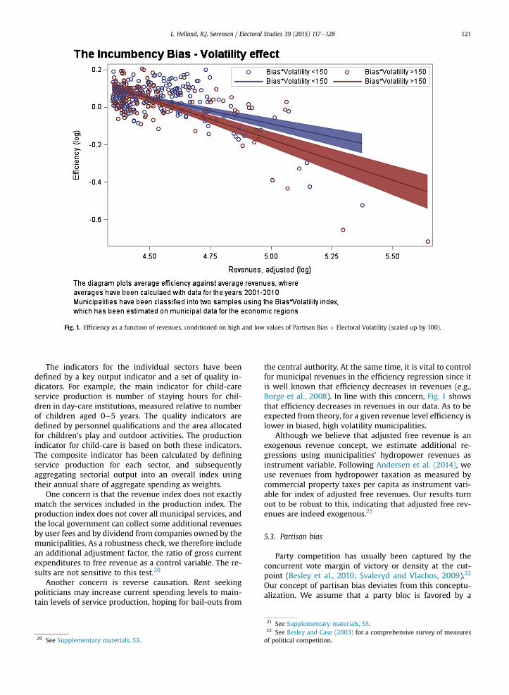
Fig. 1. Efficiency as a function of revenues, conditioned on high and low values of Partisan Bias � Electoral Volatility (scaled up by 100).

L. Helland, R.J. Sørensen / Electoral Studies 39 (2015) 117e128 121

The indicators for the individual sectors have beendefined by a key output indicator and a set of quality in-dicators. For example, the main indicator for child-careservice production is number of staying hours for chil-dren in day-care institutions, measured relative to numberof children aged 0e5 years. The quality indicators aredefined by personnel qualifications and the area allocatedfor children's play and outdoor activities. The productionindicator for child-care is based on both these indicators.The composite indicator has been calculated by definingservice production for each sector, and subsequentlyaggregating sectorial output into an overall index usingtheir annual share of aggregate spending as weights.

One concern is that the revenue index does not exactlymatch the services included in the production index. Theproduction index does not cover all municipal services, andthe local government can collect some additional revenuesby user fees and by dividend from companies owned by themunicipalities. As a robustness check, we therefore includean additional adjustment factor, the ratio of gross currentexpenditures to free revenue as a control variable. The re-sults are not sensitive to this test.20

Another concern is reverse causation. Rent seekingpoliticians may increase current spending levels to main-tain levels of service production, hoping for bail-outs from

20 See Supplementary materials, S3.

the central authority. At the same time, it is vital to controlfor municipal revenues in the efficiency regression since itis well known that efficiency decreases in revenues (e.g.,Borge et al., 2008). In line with this concern, Fig. 1 showsthat efficiency decreases in revenues in our data. As to beexpected from theory, for a given revenue level efficiency islower in biased, high volatility municipalities.

Although we believe that adjusted free revenue is anexogenous revenue concept, we estimate additional re-gressions using municipalities' hydropower revenues asinstrument variable. Following Andersen et al. (2014), weuse revenues from hydropower taxation as measured bycommercial property taxes per capita as instrument vari-able for index of adjusted free revenues. Our results turnout to be robust to this, indicating that adjusted free rev-enues are indeed exogenous.21

5.3. Partisan bias

Party competition has usually been captured by theconcurrent vote margin of victory or density at the cut-point (Besley et al., 2010; Svaleryd and Vlachos, 2009).22

Our concept of partisan bias deviates from this conceptu-alization. We assume that a party bloc is favored by a

21 See Supplementary materials, S5.22 See Besley and Case (2003) for a comprehensive survey of measuresof political competition.

L. Helland, R.J. Sørensen / Electoral Studies 39 (2015) 117e128122

partisan bias if it has a larger ‘bedrock constituency’ or ‘corebody of voters’ than its competitor.23

Short-term fluctuations in the vote margin are notnecessarily a valid indicator of partisan bias. We thereforemeasure bias in an extended time period before the rele-vant year. These data have been matched with the relevantelection periods in the 2000s, i.e. the local elections in the2001e2010 period. Bias has been measured using data onfive previous elections to municipal councils.

For each municipality, we have identified the partyblocs' minimum level of voter support over these fiveelection periods. These minimum levels are defined foreach municipality, and as a share variable. Partisan bias isdefined as the difference between the incumbent andchallenger minimum vote support. This implies that thepartisan bias has identical values for years in the sameelection period, and that variations over election periodsare limited.

The existing literature has used different strategies toidentify exogenous variation in party competition. Besleyet al. (2010) exploit the changes in the system of voterregistration in the southern US states, which ended theDemocratic Party's near monopoly position. Svaleryd andVlachos (2009) use voters support for the political partiesin the national elections in a period before a majorconsolidation of the municipality structure. They developan instrument variable for party competition by aggre-gating these data to the existing municipal structure.Sørensen (2014) has employed a similar identificationstrategy. Finally, Fiva & Natvik (2013) use municipal leveldata on national election outcomes to measure the voters'ideological preferences, and also exploit variations in thesupport for the incumbent's party bloc in the surroundingmunicipalities in the county.

In line with previous studies, our indicator of partisanbias has been measured on municipality-level voting in thenational elections (i.e. the elections to the national parlia-ment, the Storting). For this to make sense local perfor-mance should not impact on bias in national elections.Little is known about the impact of local performance onnational voting. In the election studies literature, the mainconcern seems to be the reverse, that national performanceand national campaign issues determine local election re-sults. Around 1/10 of respondents in the Local ElectionSurveys of 1995 and 1999 identified national issues as themost significant determinants of their voting (Bjørklundand Saglie, 2000:39). A majority of respondents in thelocal election survey of 1999, moreover, shared the opinionthat the local election was dominated by local issues(Bjørklund and Saglie, 2000:73). Finally, a sizable 20% ofrespondents split their party vote in the municipal andcounty elections of 1999 (Bjørklund and Saglie, 2000:53).This suggests that different considerations, or differences inparty platforms, determine the vote in the two elections for

23 Operating with blocks of parties seem warranted. Beginning with thelocal elections of 1999, political parties have increasingly chosen to enterinto formal coalition agreements. At the start of the election periods in2007 and 2011 nearly all Norwegian municipalities had formal coalitionagreements in place. See Sørensen (2014).

at least a sizable fraction of voters. Nonetheless, the cor-relation between bias in local and national elections issizable.24

By assumption, partisan voters (i.e. voters with strong(left or right) ideological preferences) do not split theirvoting at local and national elections. Partisans vote forlabels. Thus, the partisan vote shares in a given munici-pality should be the same when measured in local andnational elections. Our identifying assumption is that his-torical national election outcomes are related to efficiencyonly through their effect on the incumbency bias in theelections to the municipal councils.

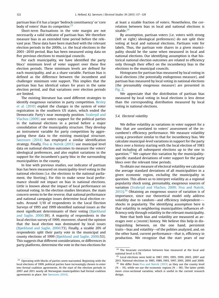
Histograms for partisan bias measured by local voting inlocal elections (the potentially endogenous measure), andpartisan bias measured by local voting in national elections(the presumably exogenous measure) are presented inFig. 2.

We appreciate that the distribution of partisan biasmeasured by local voting in local elections is less densethan the corresponding distribution measured by localvoting in national elections.

5.4. Electoral volatility

We define volatility as variations in voter support for abloc that are unrelated to voters' assessment of the in-cumbent's efficiency performance. We measure volatilityusing a procedure similar to that for incumbency bias. Wecalculatemunicipal-level variations in support for the partyblocs over a history starting with the local election of 1983and including all subsequent elections up to the one inquestion.25 We capture this variation by the municipality-specific standard deviations of voter support for the partyblocs over the relevant time periods.

To obtain ourmeasure of electoral volatility we calculatethe average standard deviations of all municipalities in agiven economic region, excluding the municipality inquestion. This allows us to interpret volatility as a regionalpopularity shock using, presumably, exogenous sources ofvariation (Svaleryd and Vlachos, 2009; Fiva and Natvik,2013).26 Obtaining an exogenous source of variation is ofimportance, since our theoretical model only addressvolatility due to randomdand efficiency independentd-shocks in popularity. The identifying assumption here isthat volatility in neighboring municipalities influences ef-ficiency only through volatility in the relevantmunicipality.

Note that both bias and volatility are measured as av-erages over a (recent) history. We believe this help in dis-tinguishing between, on the one hand, persistenttraitsdbias and volatilitydof the polities analyzed, and, onthe other hand, current performancedthat is, efficiency inproduction. We recognize that the start years of our

24 The bivariate correlation between bias measured at the local andnational level is 0.78.25 Local elections were held in 1987, 1991, 1995, 1999, 2003, 2007 and2011. National elections in 1985, 1989, 1993, 1997, 2001, 2005 and 2009.26 We differ from Fiva and Natvik (2013) as they use the county level(N ¼ 19), while we use the economic regions (N ¼ 90). The latter yieldsmore cross-sectional variation, which is useful in the current researchdesign.

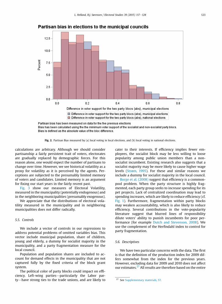
Fig. 2. Partisan Bias measured by (a) local voting in local elections, and (b) local voting in national elections.

L. Helland, R.J. Sørensen / Electoral Studies 39 (2015) 117e128 123

calculations are arbitrary. Although we should considerpartisanship a fairly persistent trait of voters, electoratesare gradually replaced by demographic forces. For thisreason alone, one would expect the number of partisans tochange over time. However, we see historical volatility as aproxy for volatility as it is perceived by the agents. Per-ceptions are subjected to the presumably limited memoryof voters and candidates. Limited memory is an argumentfor fixing our start years in the fairly recent past.

Fig. 3 show our measures of Electoral Volatility,measured in themunicipality (potentially endogenous) andin the neighboring municipalities (presumably exogenous).

We appreciate that the distributions of electoral vola-tility measured in the municipality and in neighboringmunicipalities does not differ radically.

27 See Supplementary materials, S7.

5.5. Controls

We include a vector of controls in our regressions toaddress potential problems of omitted variables bias. Thisvector include municipal population, share of children,young and elderly, a dummy for socialist majority in themunicipality, and a party fragmentation measure for thelocal council.

Population and population shares are included to ac-count for demand effects in the municipality that are notcaptured fully by the fixed criteria of the block grantsystem.

The political color of party blocks could impact on effi-ciency. Left-wing partiesdparticularly the Labor par-tydhave strong ties to the trade unions, and are likely to

cater to their interests. If efficiency implies fewer em-ployees, the socialist block may be less willing to loosepopularity among public union members than a non-socialist incumbent. Existing research also suggests that asocialist majority may be more likely to cause higher wagelevels (Strøm, 1995). For these and similar reasons weinclude a dummy for socialist majority in the local council.

Borge et al. (2008) suggest that efficiency is a common-pool problem. When the party structure is highly frag-mented, each party group seeks to increase spending for itspet projects. Lack of centralized coordination may lead tospending increases, which are likely to reduce efficiency (cf.Fig. 1). Furthermore, fragmentation within party blocksmay weaken accountability, which is also likely to reduceefficiency. Several contributions in the vote-popularityliterature suggest that blurred lines of responsibilitydilute voters' ability to punish incumbents for poor per-formance (for example Dutch and Stevenson, 2008). Weuse the complement of the Herfindahl index to control forparty fragmentation.

5.6. Descriptives

We have two particular concerns with the data. The firstis that the definition of the production index for 2009 dif-fers somewhat from the index for the previous years.However, excluding data for 2009 and 2010 does not affectour estimates.27 All results are therefore based on the entire

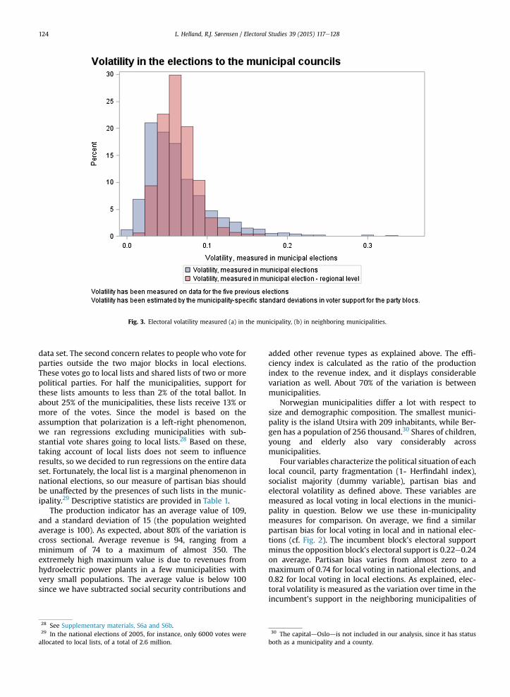
Fig. 3. Electoral volatility measured (a) in the municipality, (b) in neighboring municipalities.

L. Helland, R.J. Sørensen / Electoral Studies 39 (2015) 117e128124

data set. The second concern relates to people who vote forparties outside the two major blocks in local elections.These votes go to local lists and shared lists of two or morepolitical parties. For half the municipalities, support forthese lists amounts to less than 2% of the total ballot. Inabout 25% of the municipalities, these lists receive 13% ormore of the votes. Since the model is based on theassumption that polarization is a left-right phenomenon,we ran regressions excluding municipalities with sub-stantial vote shares going to local lists.28 Based on these,taking account of local lists does not seem to influenceresults, so we decided to run regressions on the entire dataset. Fortunately, the local list is a marginal phenomenon innational elections, so our measure of partisan bias shouldbe unaffected by the presences of such lists in the munic-ipality.29 Descriptive statistics are provided in Table 1.

The production indicator has an average value of 109,and a standard deviation of 15 (the population weightedaverage is 100). As expected, about 80% of the variation iscross sectional. Average revenue is 94, ranging from aminimum of 74 to a maximum of almost 350. Theextremely high maximum value is due to revenues fromhydroelectric power plants in a few municipalities withvery small populations. The average value is below 100since we have subtracted social security contributions and

28 See Supplementary materials, S6a and S6b.29 In the national elections of 2005, for instance, only 6000 votes wereallocated to local lists, of a total of 2.6 million.

added other revenue types as explained above. The effi-ciency index is calculated as the ratio of the productionindex to the revenue index, and it displays considerablevariation as well. About 70% of the variation is betweenmunicipalities.

Norwegian municipalities differ a lot with respect tosize and demographic composition. The smallest munici-pality is the island Utsira with 209 inhabitants, while Ber-gen has a population of 256 thousand.30 Shares of children,young and elderly also vary considerably acrossmunicipalities.

Four variables characterize the political situation of eachlocal council, party fragmentation (1- Herfindahl index),socialist majority (dummy variable), partisan bias andelectoral volatility as defined above. These variables aremeasured as local voting in local elections in the munici-pality in question. Below we use these in-municipalitymeasures for comparison. On average, we find a similarpartisan bias for local voting in local and in national elec-tions (cf. Fig. 2). The incumbent block's electoral supportminus the opposition block's electoral support is 0.22e0.24on average. Partisan bias varies from almost zero to amaximum of 0.74 for local voting in national elections, and0.82 for local voting in local elections. As explained, elec-toral volatility is measured as the variation over time in theincumbent's support in the neighboring municipalities of

30 The capitaldOslodis not included in our analysis, since it has statusboth as a municipality and a county.

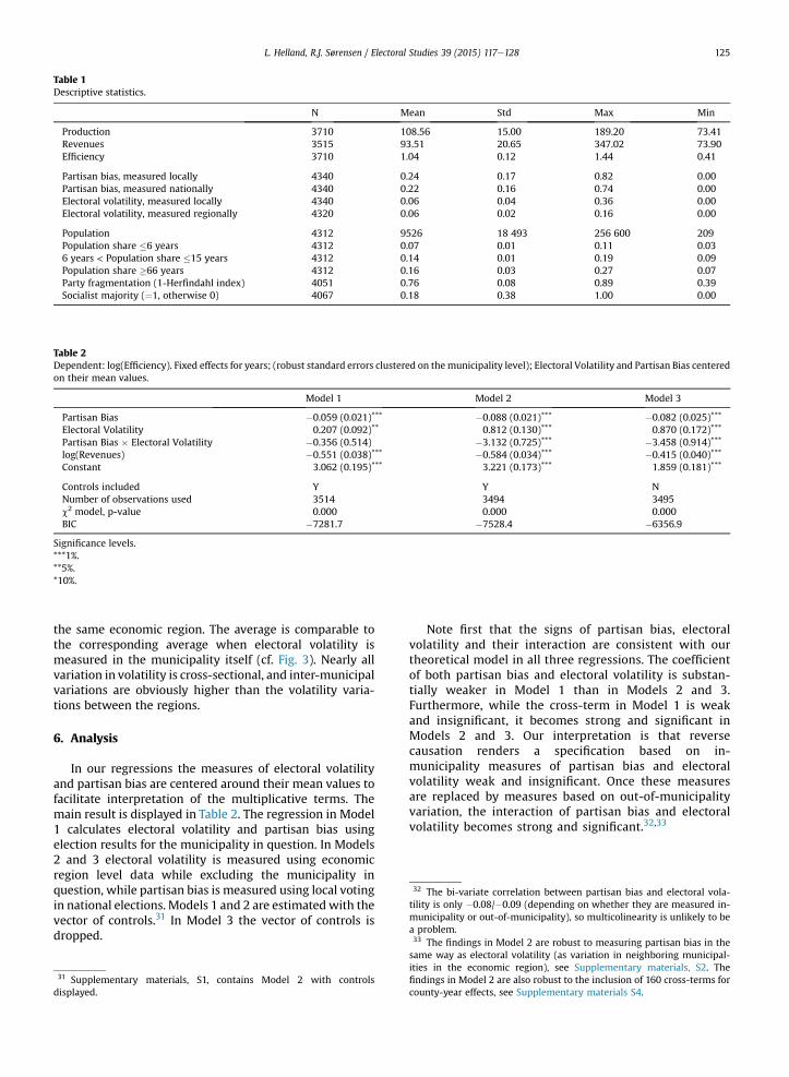
Table 2Dependent: log(Efficiency). Fixed effects for years; (robust standard errors clustered on themunicipality level); Electoral Volatility and Partisan Bias centeredon their mean values.

Model 1 Model 2 Model 3

Partisan Bias �0.059 (0.021)*** �0.088 (0.021)*** �0.082 (0.025)***

Electoral Volatility 0.207 (0.092)** 0.812 (0.130)*** 0.870 (0.172)***

Partisan Bias � Electoral Volatility �0.356 (0.514) �3.132 (0.725)*** �3.458 (0.914)***

log(Revenues) �0.551 (0.038)*** �0.584 (0.034)*** �0.415 (0.040)***

Constant 3.062 (0.195)*** 3.221 (0.173)*** 1.859 (0.181)***

Controls included Y Y NNumber of observations used 3514 3494 3495c2 model, p-value 0.000 0.000 0.000BIC �7281.7 �7528.4 �6356.9

Significance levels.***1%.**5%.*10%.

Table 1Descriptive statistics.

N Mean Std Max Min

Production 3710 108.56 15.00 189.20 73.41Revenues 3515 93.51 20.65 347.02 73.90Efficiency 3710 1.04 0.12 1.44 0.41

Partisan bias, measured locally 4340 0.24 0.17 0.82 0.00Partisan bias, measured nationally 4340 0.22 0.16 0.74 0.00Electoral volatility, measured locally 4340 0.06 0.04 0.36 0.00Electoral volatility, measured regionally 4320 0.06 0.02 0.16 0.00

Population 4312 9526 18 493 256 600 209Population share �6 years 4312 0.07 0.01 0.11 0.036 years < Population share �15 years 4312 0.14 0.01 0.19 0.09Population share �66 years 4312 0.16 0.03 0.27 0.07Party fragmentation (1-Herfindahl index) 4051 0.76 0.08 0.89 0.39Socialist majority (¼1, otherwise 0) 4067 0.18 0.38 1.00 0.00

32 The bi-variate correlation between partisan bias and electoral vola-tility is only �0.08/�0.09 (depending on whether they are measured in-municipality or out-of-municipality), so multicolinearity is unlikely to bea problem.33 The findings in Model 2 are robust to measuring partisan bias in the

L. Helland, R.J. Sørensen / Electoral Studies 39 (2015) 117e128 125

the same economic region. The average is comparable tothe corresponding average when electoral volatility ismeasured in the municipality itself (cf. Fig. 3). Nearly allvariation in volatility is cross-sectional, and inter-municipalvariations are obviously higher than the volatility varia-tions between the regions.

6. Analysis

In our regressions the measures of electoral volatilityand partisan bias are centered around their mean values tofacilitate interpretation of the multiplicative terms. Themain result is displayed in Table 2. The regression in Model1 calculates electoral volatility and partisan bias usingelection results for the municipality in question. In Models2 and 3 electoral volatility is measured using economicregion level data while excluding the municipality inquestion, while partisan bias is measured using local votingin national elections. Models 1 and 2 are estimatedwith thevector of controls.31 In Model 3 the vector of controls isdropped.

31 Supplementary materials, S1, contains Model 2 with controlsdisplayed.

Note first that the signs of partisan bias, electoralvolatility and their interaction are consistent with ourtheoretical model in all three regressions. The coefficientof both partisan bias and electoral volatility is substan-tially weaker in Model 1 than in Models 2 and 3.Furthermore, while the cross-term in Model 1 is weakand insignificant, it becomes strong and significant inModels 2 and 3. Our interpretation is that reversecausation renders a specification based on in-municipality measures of partisan bias and electoralvolatility weak and insignificant. Once these measuresare replaced by measures based on out-of-municipalityvariation, the interaction of partisan bias and electoralvolatility becomes strong and significant.32,33

same way as electoral volatility (as variation in neighboring municipal-ities in the economic region), see Supplementary materials, S2. Thefindings in Model 2 are also robust to the inclusion of 160 cross-terms forcounty-year effects, see Supplementary materials S4.

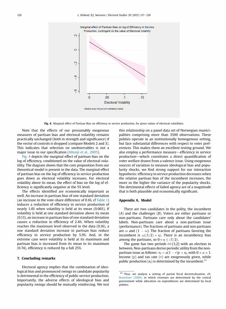
Fig. 4. Marginal effect of Partisan Bias on efficiency in service production, for given values of electoral volatilities.

L. Helland, R.J. Sørensen / Electoral Studies 39 (2015) 117e128126

Note that the effects of our presumably exogenousmeasures of partisan bias and electoral volatility remainspractically unchanged (both in strength and significance) ifthe vector of controls is dropped (compareModels 2 and 3).This indicates that selection on unobservables is not amajor issue in our specification (Altonji et al., 2005).

Fig. 4 depicts the marginal effect of partisan bias on thelog of efficiency, conditioned on the value of electoral vola-tility. The diagram shows that the core proposition from ourtheoretical model is present in the data. The marginal effectof partisan bias on the log of efficiency in service productiongoes down as electoral volatility increases. For electoralvolatility above its mean, the effect of bias on the log of ef-ficiency is significantly negative at the 5% level.

The effects identified are economically important aswell. An increase in partisan bias of one standard deviation(an increase in the vote-share difference of 0.16, cf Table 1)induces a reduction of efficiency in service production ofnearly 1.4% when volatility is held at its mean (0.065). Ifvolatility is held at one standard deviation above its mean(0.13), an increase in partisan bias of one standard deviationcauses a reduction in efficiency of 2.4%. When volatilityreaches the maximum level observed in the data (0.16), aone standard deviation increase in partisan bias reduceefficiency in service production by 5.9%. And, in theextreme case were volatility is held at its maximum andpartisan bias is increased from its mean to its maximum(0.74), efficiency is reduced by a full 25%.

34 Thus, we analyze a setting of partial fiscal decentralization, cfr.Brueckner (2009), in which revenues are determined by the centralgovernment while allocation on expenditures are determined by localpolities.

7. Concluding remarks

Electoral agency implies that the combination of ideo-logical bias and pronounced swings in candidate popularityis detrimental to the efficiency of public service production.Importantly, the adverse effects of ideological bias andpopularity swings should be mutually reinforcing. We test

this relationship on a panel data set of Norwegian munici-palities comprising more than 3500 observations. Thesepolities operate in an institutionally homogenous setting,but face substantial differences with respect to voter pref-erences. This makes them an excellent testing ground. Wealso employ a performance measuredefficiency in serviceproductiondwhich constitutes a direct quantification ofvoter welfare drawn from a valence issue. Using exogenoussources of variation to measure ideological bias and popu-larity shocks, we find strong support for our interactionhypothesis: efficiency in service production decreaseswhenthe relative partisan bias of the incumbent increases, themore so the higher the variance of the popularity shocks.The detrimental effects of failed agency are of a magnitudethat is both plausible and economically significant.

Appendix A. Model

There are two candidates in the polity, the incumbent(A) and the challenger (B). Voters are either partisans ornon-partisans. Partisans care only about the candidates'labels. Non-partisans care about a non-partisan issue(performance). The fractions of partisans and non partisansare u and (1 � u). The fraction of partisans favoring theincumbent is uðð1=2Þ þ hÞ. There is an incumbency biasamong the partisans, so 0< h � ð1=2Þ.

The game has two periods t2{1,2} with an election inbetween.Non-partisans derive periodic utility from thenon-partisan issue as follows: vt ¼ a(1 � t)y þ xt, with 0 < a < 1.Income (y) and tax rate (t) are exogenously given, whilepublic production (xt) is determined by the incumbent.34

L. Helland, R.J. Sørensen / Electoral Studies 39 (2015) 117e128 127

At the beginning of period one a revenue shock j2{s,1},with 0 < s < 1, hits the local economy.35 The common priorover the shock is Pr(j ¼ s) ¼ q and Pr(j ¼ 1) ¼ (1 � q). Weassume q � 1=2.36 The revenue shock is persistent (¼lastsfor two periods). The public produces according tojetty ¼ xt, with et2[0,1] representing the effort of theincumbent. Let (j¼ 1)(et¼ 1)ty≡R (production at full effortand high revenues equal R). We assume that funds cannotbe diverted for private ends.

Incumbents come in two types i2{g,b} g-types set et¼ 1unconditionally. The payoff function of b-types isub ¼ E�c(e1) þ b(E � c(e2)). E is an ”ego-rent,” while b<1 isthe discount factor. c(et) is the cost of effort function. As-sume c(0) ¼ 0, c(1) > bE and c0>0cet2[0,1]. The prior overtypes is Pr(i ¼ g) ¼ p and Pr(i ¼ b) ¼ (1 � p).

The incumbent is subject to an aggregate popularityshock d2(0,∞). The cdf of this popularity shock is H(d),with corresponding density h(d). The density is assumed tobe symmetric and unimodal. Type and productivity aredrawn at the beginning of period one, and revealed to theincumbent only. The realization of the aggregate popularityshock is revealed to everyone in the election. The structureof the game (including prior distributions) is commonknowledge.

Non-partisans use a cut-off rule in their voting: if thechallenger and the incumbent are equally popular and theupdate of a g-type is at least as great as the prior, theincumbent is kept, otherwise she is ousted.

We now show that existence of a pooling equilibrium inwhich b-type incumbents can, to some extent, be disci-plined by voters. In the pooling equilibrium, lazy politiciansonly exert an effort in the initial period if revenues are highand the probability of reelection is not too low. The prob-ability of reelection is a function of incumbent behavior inthe initial period, partisan bias, and the density of thepopularity shock. In particular, we show that the support ofthe pooling equilibrium shrinks when the relative partisanbias of the incumbent increases, andmore so the higher thevariance of the popularity shock.

Proposition 1. For q � 1=2 and s> k≡ð1� qÞð1� pÞ=1� p

ð1� qÞ

a) a pooling equilibrium exists in which b-types mimic g-types when revenues are high

b) support of this pooling equilibrium is greater in theabsence of partisan voters

Last period behavior is trivial: g-types choose full effort,b-types choose zero. Consider updates prior to election.Note first that full effort is dominated for b-types. Let H0

represent reelection probability with no effort, and HR

reelection probability with full effort. The no effort condi-tion is E þ H0bE > E � c(1) þ HRbE, which can also bewritten c(1) > bE(HR � H0). The last condition is satisfied by

35 Alternatively, we may interpret the shock as an exogenous produc-tivity shock.36 This assumption simplifies the analysis, by removing a hybrid equi-librium in which players randomize over actions.

the assumption that c(1) > bE, and the fact that (HR � H0)2[�1,1]. Thus, no effort dominates full effort so thatPr(i ¼ gjx1 ¼ R) ¼ 1.

By the definition of types Pr(i ¼ gjx1 ¼ 0) ¼ 0. Whatabout Pr(i ¼ gjx1 ¼ sR)? Let l denote the probability that ab-type produces sR when j ¼ 1. Then Prði ¼ gjx1 ¼ sRÞ ¼ðpq=pqþ ð1� pÞð1� qÞlÞ≡P. We conclude that reputationis maintained or improved ( i.e. P�p�0) if l � ðq=1� qÞ,which is true under the assumption that q � 1=2.

Let a non-partisan voter j reelect the incumbent ifð1=2Þ þ dþ v2ðjÞPrði ¼ gjx1Þ � v2ðjÞp. Assume we are in apooling equilibrium where b-types set (x1 ¼ sRjj ¼ 1). Weneed to consider three cases.

Case 1. Assume x1 ¼ 0. Then Pr(i ¼ gjx1 ¼ 0) ¼ 0 andPr(j ¼ sjx1 ¼ 0) ¼ 1. The reelection condition of voter jreduces to ð1=2Þ þ d � psR. Aggregating over voters, thecondition for the incumbent to survive elections now be-comes uðð1=2Þ þ hÞ þ ð1� uÞðð1=2Þ þ d� psRÞ> ð1=2Þ0d

< ðuh=1� uÞ � psR. Write the incumbent bias asðuh=1� uÞ≡q. Given our distributional assumptions on thepopularity shock, an incumbent that delivers x1 ¼ 0 isreelected with probability H0(q � psR).

Case 2. Assume x1 ¼ R. Then Pr(i ¼ gjx1 ¼ R) ¼ 1 andPr(j ¼ 1jx1 ¼ R) ¼ 1. The reelection condition of voter jbecomes ð1=2Þ þ dþ R � pR, or ð1=2Þ þ dþ Rð1� pÞ � 0.Aggregating as in case (1), the probability of incumbencysurvival after observing x1 ¼ R becomes HR(q þ R(1 � p)).

Case 3. Assume x1 ¼ sR. Then P�p andPr(j ¼ sjx1 ¼ sR) ¼ Pr(i ¼ gjx1 ¼ sR) ¼ P. The reelectioncondition of voter j then becomes ð1=2Þ þ dþPsR � p

½PsRþ ð1�PÞR�, or ð1=2Þ þ dþ R½sð1� pÞPþ ð1�PÞp�� 0. The probability of the incumbent surviving after hav-ing produced x1 ¼ sR is HsR(q þ R[s(1�p)P þ (1�P)p]).

For the problem to be well behaved we needHR > HsR > H0. We now show that this ordering requires0 < k < s < 1. Rearranging we find that HR > HsR as long ass < 1, which is true by assumption. Furthermore, HsR > H0 ifs > k. Note that k falls quickly with both q2½1=2;1Þ andp2(0,1), and approaches its maximum value k ¼ 1=2 asp/0 while q ¼ 1=2. Thus, for a large range of values on p

and q requiring HsR > H0 is undemanding. Inwhat follows itis assumed that this requirement is met. Comparing the lastexpressions in cases (1) and (2), it is immediate thatHR >H0

for all permissible values.

Proof. For a b-type to be willing to produce (x1 ¼ sRjj¼ 1)the following inequality will have to be satisfiedE� c(s)þHsR(qþ R[s(1�p)Pþ (1�P)p])bE�EþH0(q�psR)bE, which can be rewritten as a pooling condition(A1): cðsÞ=bE�HsRðqþR½sð1�pÞPþð1�PÞp�Þ�H0ðq�psRÞ.In a world without ideology (only non-partisan voters) andno popularity shocks, it is readily seen that the poolingcondition reduces to (A2): cðsÞ=bE�1: It is evident that theright hand side of (A1) is smaller than that of (A2). -

Remark: Electoral uncertainty and incumbency biasclearly reduce the support of an equilibrium in whichshirking can be disciplined. The derivative of the differenceon the RHS of (A1) wrt q is proportional to: hsR(q þ R[s(1 � p)P þ (1�P)p]) � h0(q � psR). Noting that [s(1 � p)

L. Helland, R.J. Sørensen / Electoral Studies 39 (2015) 117e128128

P þ (1 � P)p] > 0, the effect of incumbency bias (q) can beclarified. For q< q0 ¼ ð1=2ÞR½Pðp� sð1� pÞÞ � pð1� sÞ�,increased bias expands the support of the pooling equi-librium. For q>q0 increased bias contracts the support of thepooling equilibrium. Further to this, the higher the stan-dard deviation of the h(d) distribution (the more uncer-tainty there is in the voting mechanism), the less likelydiscipline becomes (the smaller is the support of a poolingequilibrium) for given values of q.

Appendix B. Supplementary data

Supplementary data related to this article can be foundat http://dx.doi.org/10.1016/j.electstud.2015.05.002.

References

Alesina, A., Baqir, R., Easterly, W., 1999. Public goods and ethnic divisions.Q. J. Econ. 114, 1243e1284.

Altonji, J., Elder, T., Taber, C., 2005. Selection on observed and unobservedvariables: assessing the effectiveness of catholic schools. J. Polit. Econ.113 (1), 151e184.

Andersen, J., Fiva, J., Natvik, G., 2014. Voting when the stakes are high. J.Public Econ. 110, 157e166.

Austen-Smith, D., Banks, J., 1989. Electoral accountability and in-cumbency. In: Ordeshook, P. (Ed.), Models of Strategic Choice inPolitics. The University of Michigan Press, Ann Arbor.

Banks, J., Sundaram, R., 1993. Adverse selection and moral Hazard in arepeated elections model. In: Barnett, W., Hinich, M., Schofield, N.(Eds.), Political Economy: Institutions, Competition, and Representa-tion. Cambridge University Press, Cambridge.

Barro, R., 1973. The control of politicians: an economic model. PublicChoice 14, 19e42.

Besley, T., Case, A., 2003. Political institutions and policy choices: evi-dence from the United States. J. Econ. Lit. 41 (1), 7e73.

Besley, T., 2006. Pricipled Agents. The Political Economy of Good Gov-ernment. Oxford University Press, Oxford.

Besly, T., Persson, T., Sturm, D., 2010. Political competition, policy andgrowth: theory and evidence from the US. Rev. Econ. Stud. 77 (4),1329e1352.

Bjørklund, T., Saglie, J., 2000. Lokalvalget 1999. Oslo: ISF-rapport 2000:12.Borge, L.-E., Falch, T., Tovmo, P., 2008. Public sector efficiency: the roles of

political and budgetary institutions, fiscal capacity and democraticparticipation. Public Choice 136, 475e495.

Brueckner, J., 2009. Partial fiscal decentralization. Reg. Sci. Urban Econ. 39,23e32.

Bruns, C., Himmler, O., 2011. Newspaper circulation and local governmentefficiency. Scand. J. Econ. 113 (2), 470e492.

Bun, M., Harrison, T., 2014. OLS and IV Estimation of Regression ModelsIncluding Endogenous Interaction Terms. Working paper. Universityof Amsterdam, Department of Economics & Econometrics.

Cheibub, J., Przeworski, A., 1999. Democracy, elections, and accountabilityfor economic outcomes. In: Przeworski, A., Stokes, S., Manin, B. (Eds.),Democracy, Accountability, and Representation. Cambridge Univer-sity Press, Cambridge.

Dalton, R., 2002. The decline of party identification. In: Dalton, R.,Wattenberg, M. (Eds.), Parties without Partisans: Political Change inAdvanced Industrial Democracies. Oxford University Press, Oxford.

Drummond, A., 2006. Electoral volatility and party decline in Westerndemocracies: 1970e1995. Polit. Stud. 54 (3), 628e647.

Duch, R., Stevenson, R., 2008. The Economic Vote: How Political andEconomic Institutions Condition Election Results. Cambridge Uni-versity Press, Cambridge.

Easterly, W., Levine, R., 1997. Africa's growth tragedy: policies and ethnicdivisions. Q. J. Econ. 112, 1203e1250.

Ferejohn, J., 1986. Incumbent performance and electoral control. PublicChoice 50, 5e25.

Fearon, J., 1999. Electoral accountability and the control of politicians:selecting good types versus sanctioning poor performance. In:Przeworski, A., Stokes, S., Manin, B. (Eds.), Democracy, Accountability,and Representation. Cambridge University Press, Cambridge.

Fiva, J., Natvik, G., 2013. Do re-election probabilities influence public in-vestment? Public Choice 157, 305e331.

Helland, L., Monkerud, L., 2013. Electoral Agency in the lab: learning tothrow out the rascals. J. Theor. Polit. 25 (2), 214e233.

Hix, S., Marsh, M., 2007. Punishment or protest? Understanding Europeanparliament elections. J. Polit. 69 (2), 495e510.

Johansson, E., 2003. Intergovernmental grants as a tactical instrument:empirical evidence from Swedish municipalities. J. Public Econ. 87(5e6), 883e915.

Maskin, E., Tirole, J., 2004. The politician and the judge: accountability ingovernment. Am. Econ. Rev. 94 (4), 1034e1054.

Pedersen, M., 1979. The dynamics of European party systems: changingpatterns of electoral volatility. Eur. J. Polit. Res. 7 (1), 1e21.

Persson, T., Tabellini, G., 2000. Political Economics. The MIT-Press, Cam-bridge Mass.

Petterson-Lidbom, P., 2006. Testing Political Agency Models. WorkingPaper. Department of Economics, Stockholm University.

Polo, M., 1998. Electoral Competition and Political Rents. InnocenzoGaspari Institute for Economic Research, Milano (unpublished).

Strøm, B., 1995. Envy, fairness and political influence in local governmentwage determination: evidence from Norway. Economica 62,382e409.

Sørensen, R., 2014. Political competition, party polarization, and govern-ment performance. Public Choice 161, 427e450.

Svaleryd, H., Vlachos, J., 2009. Political rents in a non-corrupt democracy.J. Public Econ. 93, 355e372.

Svensson, J., 1997. The Control of Public Policy: Electoral Competition,Polarization and Primary Elections. The World Bank, Washington DC(unpublished).

Svensson, J., 1999. Aid, growth, and democracy. Econ. Polit. 11 (3),275e297.