PARTIEl À - espace.etsmtl.caespace.etsmtl.ca/824/1/BROWN_Mark.pdf · Cependant. même si le...

Reproduced with permission of the copyright owner. Further reproduction prohibited without permission.

ÉCOLE DE TECHNOLOGIE SUPÉRIEURE UNIVERSITÉ DU QUÉBEC

MÉMOIRE DE 21 CRÉDITS PRÉSENTÉ À L•ÉCOLE DE TECHNOLOGIE SUPÉRIEURE

COMME EXIGENCE PARTIEl 1 E À L ·oBTENTION DE LA

MAÎTRISE GÉNIE DE LA CONSTRUCI10N M.lng.

PAR MARK BROWN

MANAGING THE REHABILITATION OF FOREST ROADS USING HISTORICAL DAIL Y ROUGHNESS DATA COLLECTED BY THE OPTI-GRADE®

SYSTEM

MONTRÉAL. AOÛT 2002

© droits réservés de Mark Brown


Mark Brown

Gestioa de la réfection des chemiDs forestien à l'aide de données historiques qaotidieaaes sur la rugosité recueillies avec le système Opti-Grade*

Pour gérer l'entretien des chemins forestiers, l'Institut canadien de recherches en génie forestier (FERIC) a mis en application Opti-Grade, un système de gestion de nivelage, qui a permis aux entreprises forestières d'économiser entre 15 et 35% de leurs coûts d'entretien des chemins. En plus d'être un outil de gestion de l'entretien journalier, les donnés d'Opti-Grade peuvent être utilisées pour améliorer la gestion de la réfection des chemins forestiers.

Pour confirmer la fiabilité des données du système Opti-Grade on a étudié la répétabilité des mesures obtenues. Divers systèmes de gestion de chaussée disponibles ont été évalués pour être utilisés avec les données du système Opti-Grade pour gérer la réfection des chemins. Comme aucun système ne convenait parfaitement aux besoins de l'industrie forestière, on a décidé d'élaborer un système de gestion de la réfection des chemins capable d'isoler les tronçons de chemins à réparer et de déterminer la date d'exécution de ces travaux.


THIS MASTER W AS EV ALUATED BY A JURY COMPOSED OF:

• M. Gabriel J. Assaf. director of researcb Département de génie de la construction at 1•École de technologie supérieure

• M. Yves Provencher. co-director master Forest Engineering Researcb lnstitute of Canada (FERIC)

• Michèle St-Jacques. president of the jury and professor Département de génie de la construction att•Ecole de technologie supérieure

• Dr. Maarouf Saad. professor Département de génie électrique

IT WAS THE TOPIC OF PRESENTATION BEFORE

THEJURY ANDPUBUC

JUNE 27. 2002

AT L•ÉCOLE DE TECHNOLOGIE SUPÉRIEURE


GESTION DE LA RÉFEcriON DES CHEMINS FORESTIERS À L'AIDE DE DONNÉES mSTORIQUES QUOTIDIENNES SUR LA RUGOSITÉ

RECUEILLIES AVEC LE SYSTÈME OPTI-GRADE®

Mark Brown

Sommaire

Pour gérer l'entretien des chemins forestiers. l'Institut canadien de recherches en génie forestier (FERIC) a mis en application Opti-Grade. un système de gestion de nivelage. qui a permis aux entreprises forestières d•économiser entre 15 et 35% de leurs coûts d'entretien des chemins. En plus d•être un outil de gestion de l'entretien journalier. les données d•Opti-Grade peuvent être utilisées pour améliorer la gestion de la réfection des chemins forestiers.

Pour confirmer la fiabilité des données du système Opti-Grade nous avons étudié la répétabilité des mesures obtenues. Divers systèmes de gestion de chaussée disponibles ont été évalués pour être utilisés avec les données du système Opti-Grade afin de gérer la réfection des chemins. Comme aucun système ne convenait parfaitement aux besoins de l'industrie forestière. on a décidé d•élaborer un système de gestion de la réfection des chemins capable d·isoler les tronçons de chemins à réparer et de déterminer la date d • exécution de ces travaux.


MANAGING THE REHABILITATION OF FOREST ROADS USING BISTORICAL DAIL Y ROUGHNESS DATA COLLECfW BY THE OPfi

GRADE. SYSTEM

Mark Brown

Abstract

The forest industry represents an important contributor to the Canadian economy. generating $44.2 billion worth of exports per year and providing direct jobs to more than 350 000 Canadians. As witb most industries in the world tbat are dealing witb the issue of globalization. the Canadian forest industry faces increased competition for international markets. and this competition generates an ever-increasing need to control costs and spend budgets efficiently to obtain the best-possible results. One important area of operational costs for the forest industry involves forest roads. wbicb represent about 15% of total in-woods operational costs.

The key to controlling road costs lies in obtaining timely information on the roads. and this concept underlies the implementation of any pavement management system. ln the case of forest roads. years of evolution witbin the industry bave not been accompanied by efforts to obtain and update information about road conditions and management. Wben trucks and thus roads were frrst introduced in the forest industry. they were used solely for short-distance transport. so road networks were small and those in charge of maintenance could easily keep track of the condition and management of their roads. As it became necessary to extend the road networks for longer transportation distances and as road managers took on responsibility for multiple tasks in addition to road management. their personal knowledge of the roads inevitably decreased greatly. Consequently. the maintenance of road networks feil into a pattemed approacb in whicb every section of the road received the same maintenance. regardless of that section·s performance. Similarly. road rehabilitation suffers from a less tban optimal approacb; with no way to justify the need for a budget to perform road rehabilitation and no way to objectively identify where rehabilitation is required. road rehabilitation is only performed when money is left over in the budget.

To deal with these road maintenance issues. the Forest Engineering Researcb lnstitute of Canada (FERIC) bas recently implemented an effective. simple. low-cost system called Opti-Grade. This system consists of a hardware component and a software component. The hardware is installed on a haul vebicle that travels regularly across the road network. and once it bas been installed. it continuously measures road roughness. This data is then transferred daily to the software. whicb analyzes it based on userdefined criteria to identify wbere grading is required. This focused approach to road maintenance bas allowed the eighteen Canadian forestry operations that have


iii

implemented Opti-Grade in 2001 to save between 15 and 35% on their road maintenance costs. However, although Opti-Grade bas significantly improved road maintenance, additional efforts must be made to improve forest road rehabilitation management.

The large database of road roughness values being created and stored by OptiGrade provides a natural basis for a future road rehabilitation management system (RMS). To confrrm the reliability of Opti-Grade's data for use in such an RMS. the repeatability of the Opti-Grade system • s measurements was tested and it was confrrmed that the level of repeatability was adequate. Through a literature search, various currently available pavement management systems suitable for rehabilitation management in the forest industry based on Opti-Grade data were identified and evaluated. It was concluded that no existing system was weil suited to the needs of the forest industry and the use of Opti-Grade data. Therefore, a RMS was developed that wouJd identify where and when rehabilitation should be performed.

The Opti-Grade data suggest that the roughness of forest roads is very variable over short times and distances and thus, this data is not directly usable for the development of road performance curves. Instead, it was determined that the best method for modeling road performance based on Opti-Grade data would be based on Markov chains. To do this analysis, sections of the road network were divided into families, based on road geometry. This typically gives three or four families per road network. Markov matrices are theo developed based on the Opti-Grade data for each segment of road within a family; subsequent! y, a Markov matrix is devised for each age group within a family of roads. Using these predictive models, the road user and maintenance costs are simuJated using Monte Carlo simulations summed to determine the total annual cost for each age group of road. The total 5-year costs of six different scenarios are provided to the manager; the chosen scenarios involved doing no rehabilitation, and perfonning rehabilitation in years 1 through 5. The road manager can theo generale a 5-year road rehabilitation plan in which the location and time of the rehabilitation bas been economically optimized.


GESTION DE LA RÉFEcriON DES CHEMINS FORESTIERS À L'AIDE DE DONNÉES HISTORIQUES QUOTIDIENNES SUR LA RUGOSITÉ

RECUEILLIES AVEC LE SYSTÈME OPfi-GRADE®

Mark Brown

Résumé

L • industrie forestière constitue un volet important de l'économie canadienne, avec 44.2 milliards$ d'exportations par année et plus de 350 000 emplois directs au Canada. Dans un contexte de mondialisation, l'industrie forestière canadienne, à l'instar de la plupart des industries dans le monde, fait face à une concurrence accrue sur les marchés internationaux. Compte tenu de cette concurrence, les industries doivent sans cesse limiter leurs coûts et utiliser efficacement leurs budgets de façon à optimiser leurs activités. Dans l'industrie forestière, les chemins forestiers constituent l'un des postes importants du budget d'exploitation- environ 15% des dépenses totales en forêt.

La meilleure façon de limiter les coûts inhérents aux chemins forestiers consiste à obtenir en temps opportun de l'information sur ceux-ci ; or, ce concept sous-tend la mise en œuvre d'un système de gestion des chaussées. Dans le cas des chemins forestiers, l'industrie n ·a jamais, au m de son évolution. consenti les efforts nécessaires pour recueillir de l'information sur l'état et la gestion des chemins el pour mettre cette information à jour. Quand les camions et les chemins ont fait leur apparition dans l'industrie forestière, ils ne servaient qu ·au transport sur de courtes distances ; le réseau forestier était de faible envergure, et les responsables de son entretien pouvaient facilement faire le suivi de l'état et de la gestion des chemins. Lorsqu'on a étendu le réseau forestier pour couvrir de plus longues distances, les gestionnaires de chemins, qui se sont vus confier plusieurs autres tâches en plus de la gestion des chemins, ne pouvaient plus être aussi bien informés de l'état du réseau. Ds ont donc dû adopter une approche globale en matière d'entretien selon laquelle chaque section de chemin forestier reçoit le même entretien, peu importe son état. La réfection des chemins est, elle aussi gérée selon une approche quelque peu désuète. Comme on ne dispose pas de moyens pour justifier l'allocation de fonds pour la réfection des chemins et que l'on ne peut déterminer objectivement les endroits à réparer. la réfection des chemins n • est effectuée qu'à partir des surplus budgétaires.

Pour régler les problèmes associés à l'entretien des chemins, l'Institut canadien de recherches en génie forestier (FERIC) a récemment mis en application un système efficace, simple et peu coûteux appelé Opti-Grade, qui est constitué d'un composant matériel et d'un composant logiciel. Le composant matériel, installé sur un vemcule de transport qui sillonne régulièrement le réseau forestier, mesure sans interruption la rugosité des chemins. Les données recueillies sont transférées chaque jour au composant logiciel, qui les analyse en fonction de critères définis par l'utilisateur pour établir les


v

endroits nécessitant un nivellement. Cette approche ciblée en matière d'entretien des chemins a permis à dix-huit entreprises forestières canadiennes, qui ont mis en application le système Opti-Grade au cours de la dernière année, d'économiser entre 15 et 35 % de leurs coûts d'entretien des chemins. Cependant. même si le système OptiGrade a amelioré l'entretien des chemins de façon significative, il faut consentir d'autres efforts pour améliorer la gestion de la réfection des chemins forestiers.

L'importante base de données sur la rugosité des chemins créée avec le système Opti-Grade constitue un point de départ logique pour un futur système de gestion de la réfection des chemins. Pour confmner la fiabilité des données du système Opti-Grade avant de les appliquer à un système de gestion de la réfection des chemins, on a étudié la répétabilité des mesures obtenues et on constaté que le niveau de la répétabilité était adéquat. En examinant la littérature à ce sujet, on a ensuite relevé et évalué les divers systèmes de gestion de chaussée disponibles que l'on pourrait utiliser pour effectuer la gestion de la réfection des chemins avec les données du système Opti-Grade. Comme aucun système ne convenait parfaitement aux besoins de l'industrie forestière et aux données du système Opti-Grade, on a décidé d'élaborer un système de gestion de la réfection des chemins capable d'isoler les tronçons de chemins à réparer et de déterminer la date d'exécution de ces travaux.

Les données du système Opti-Grade indiquent que la rugosité des chemins forestiers varie passablement sur de courtes périodes et de courtes distances. On ne peut donc utiliser directement ces données pour l'élaboration de courbes de rendement des chemins. On a par ailleurs déterminé que la meilleure méthode pour modéliser le rendement des chemins à partir des données du système Opti-Grade était d'utiliser l'analyse en chaînes de Markov. Pour effectuer cette analyse, on a divisé des segments de chemin en familles d'après la géométrie des chemins. Les résultats obtenus sont d'ordinaire trois ou quatre familles par réseau de chemins. On a ensuite élaboré des matrices de Markov à partir des données du système Opti-Grade pour chaque segment de chemin d'une même famille, puis on a conçu une matrice de Markov pour chaque catégorie d'âge d'une même famille des chemins. Grâce à ces modèles de prévision, on simule les coûts en entretien et en utilisation des chemins à 1' aide de la méthode de Monte Carlo, puis on additionne les résultats pour déterminer le coût total annuel pour chaque catégorie d'âge de chemin. Les coûts totaux sur 5 ans de six scénarios différents sont ensuite fournis au gestionnaire. Les scénarios retenus sont les suivants: ne faire aucune réfection ou effectuer des travaux de réfection au cours de l'année l, 2, 3, 4 ou 5. Le gestionnaire du réseau forestier peut alors produire un plan quinquennal de réfection des chemins dans lequel les secteurs et la période de réfection ont été optimisés sur le plan économique.


ACKNOWLEDGMENTS

The author would like to thank his research director for this project. Dr. Gabriel J.

Assaf, for his valuable direction. advise and encouragement. He would also like to thank

Yves Provencher, co-director of research for this project. for his continuous support.

advice. and encouragement through out the entire project.

In addition, the author feels it important to thank Dr. Joseph A. Nader, researcher

and mathematician at FERIC, for his explanations and support during the statistical

analysis of the data.

Without the complete support and cooperation of the Forest Engineering Research

Institute of Canada (FERIC) in the initiation and realization of this project. it would not

have been possible. For this excellent support. the author would like to thank the

management and staff of FERIC.

For their support and valuable work with the Opti-Grade road maintenance

management system, the author would like to thank the FERIC Opti-Grade team for

their help and their excellent work in making Opti-Grade a success. The team includes

Andrew Hickman, technician; Steve Mercier, researcher; Marc Arsenault, programmer;

Brent McPhee, technician; Yves Provencher, program leader for roads and


vii

transportation; Pierre Turcotte. program leader for special technologies; and Jan

Michaelsen. researcher.

The quality of the writing in this thesis would not have been near the quality it is

without editing support of Geoff Hart. editor at FERIC.

Finally. the following forest companies were instrumental in project by allowing

FERIC to analyze their Opti-Grade data:

Domtar loc.

Abitibi-Consolidated loc.

Tembec loc.


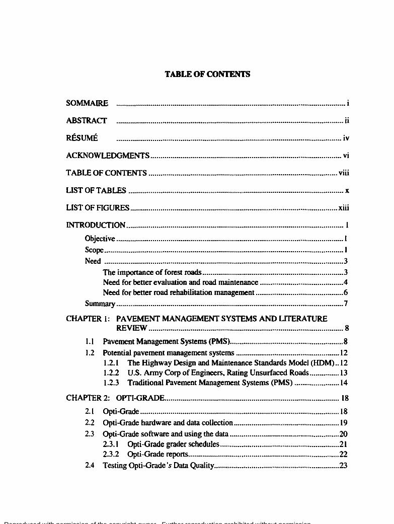
TABLE OF CONTENTS

SOMMAIRE ................................................................................................................... i

ABSTRACf .................................................................................................................. ii

RÉSUMÉ ................................................................................................................. iv

ACKNOWLEDGMENTS ................................................................................................ vi

TABLE OF CONTENTS ............................................................................................... viii

UST OF TABLES ............................................................................................................ x

UST OF FIGURES ........................................................................................................ xiii

INTRODUCTION ............................................................................................................. 1

Objective .................................................................................................................. 1

Scope ........................................................................................................................ 1

Need ........................................................................................................................ 3

The importance of forest roads .........•...•....•......................•............................. 3 Need for better evaluation and road maintenance ......................................... .4 Need for better road rehabilitation management ............................................ 6

Summary .................................................................................................................. 7

CHAPTER 1: PAVEMENT MANAGEMENT SYSTEMS AND UTERATURE REVIEW .................................................................................................. 8

1.1 Pavement Management Systems (PMS) ......................................................... 8

1.2 Potential pavement management systems .................................................... 12 1.2.1 The Highway Design and Maintenance Standards Mode1 (HOM) .. 12 1.2.2 U.S. Army Corp of Engineers. Rating Unsurfaced Roads ............... 13 1.2.3 Traditional Pavement Management Systems (PMS) ....................... 14

CHAP'fER 2: OPTI-GRADE ........................................................................................ 18

2.1 Op ti -Grade .................................................................................................... 18

2.2 Opti -Grade hardware and data collection ..................................................... 19

2.3 Opti-Grade software and using the data ....................................................... 20 2.3.1 Opti-Grade grader schedules ............................................................ 21 2.3 .2 Opti-Grade reports ............................................................................ 22

2.4 Testing Opti-Grade's Data Quality ............................................................... 23


ix

2.4.1 Repeatability of Opti-Grade data ..................................................... 24

2.5 Test design .................................................................................................... 25

2.6 Data analysis ................................................................................................. 26

CHAPTER 3: REHABIT..IT A TION MANAGEMENT wrrH OPTI-GRADE ............ 34

3.1 Data provided by Opti-Grade and how it can be modeled and simulated for rehabilitation management ..................................................... 34 3.1.1 Context ............................................................................................. 34 3.1.2 Selecting modeling and simulation methods .................................... 37

3.2 The madel for rehabilitation management .................................................... 38

3.3 Additional information for rehabilitation decisions .................................... .42 3.3.1 Familles ............................................................................................ 43 3.3 .2 Costs for simulation ......................................................................... 44

3.4 Simulation with the models .......................................................................... 46

3.5 Feedback loop and continuai improvement of the models ........................... 50

3.6 Example of simulation .................................................................................. 51 3.6.1 The Madel: Transition matrices ....................................................... 51 3.6.2 Random number prediction tables .................................................... 54 3.6.3 Simulation ........................................................................................ 56 3.6.4 Results and extrapolations to produce decision matrices ................. 65 3.6.5 I>ecision Matrices ............................................................................. 67 3.6.6 I>ecisions based on decision matrices .............................................. 73

CHAP'fER 4: RECOMMENDA TIONS ....................................................................... 15

CONCLUSION ............................................................................................................... 77

APPENDIX A: REPEA T ABILITY TESTS FOR OPTI-GRADE .................................. 78

REFERENCES . . . . .... .•••..... .. .•. . . . . . .. .. . .. ... . . .•. ..••... .•..•... .. ... .. . . . . ... . .. .•.• ... .. . . .. •. .... .. .. . . . .. . . . •• . . . . . 89


LISfOFTABLES

Table 1 An example of Opti-Grade data. including roughness measurements ........................................................................................ 20

Table II Test data that was collected on the two road sections .......................... 26

Table rn Repeatability tests for test section l at 40 kmlh ................................... 28

Table IV Repeatability of roughness measurements for road section l at three speeds .....••••.•......•.•..••.••••.••••••.••..•••••••.••.•....•..•••••..•..•........••••..•..... 30

Table V Repeatability of roughness measurements for road section 2 at three speeds •••••...•.•..•••••.••••.•.••••••.•.•••.••••••.•••••.•..••.•.•.••••••.•........••••••••••.•. 30

Table VI Magnitude of the variation in roughness measurements at three speeds .••••.•.•.••..••••.•.•..•.•.••••••..••••..•.•••••.•••.•..•.•.••.•.••••.••••••••.•.•....•..•••••••.•. 32

Table Vll Example of a transition matrix built from Opti-Grade data .................. 40

Table Vlli Example of a grading probability table ................................................ .4l

Table IX Example of a transition matrix built from Opti-Grade data combined with feedback on whether grading was perfonned ............. .42

Table X Example of a random-number prediction table based on Monte Carlo simulations .................................................................................. 4 7

Table XI Example of a decision matrix produced by the model.. ....................... .49

Table Xll Transition matrix model for a road that bas been rehabilitated within the last year ................................................................................ 51

Table XID Transition matrix model for a road that was rehabilitated l to 2 years ago ............................................................................................... 52

Table XIV Transition matrix model for a road thal was rehabilitated 2 to 3 years ago ............................................................................................... 52

Table XV Transition matrix model for a road thal was rehabilitated 3 lo 4 years ago ............................................................................................... 52

Table XVI Transition matrix model for a road that was rehabilitated 4 to 5 years a go ............................................................................................... 53

Table XVTI Transition matrix model for a road thal was rehabilitated 5 to 6 years a go ............................................................................................... 53

Table XVIII Transition matrix model for a road thal was rehabilitated 6 to 7 years a go ............................................................................................... 53

Table XIX Transition matrix model for a road that was rehabilitated 7 to 8 years ago ............................................................................................... 54


xi

Table XX Transition matrix model for a road that was rehabilitated 8 to 9 years ago ............................................................................................... 54

Table XXI Random number prediction table for a road rehabilitated within the last year if its current state is level 1 ..................................................... 55

Table xxn Random number prediction table for a road rehabilitated within the last year if its current state is level 2 ..................................................... 55

Table XXID Random number prediction table for a road rehabilitated within the last year if its current state is level 3 ..................................................... 56

Table XXN Results of a 150-day simulation for a road that was rehabilitated within the last year at a grading cost of $65/km and with no increased user cost as a function of deteriorating road condition ......... 57

Table XXV Results of a 150-day simulation for a road that was rehabilitated within the last year at a grading cost of $65/km, with increased user costs of $10 per kilometre per day for level 2 road condition and $30 per kilometre per day for level 3 condition .................................... 61

Table XXVI Simulation results, showing annual road maintenance costs as they relate to time since last rehabilitation ................................................... 65

Table XXVll Simulation results, showing annual road maintenance plus user costs as they relate to time since last rehabilitation .............................. 66

Table XXVID Decision matrix for a road segments rehabilitated in the fast year. considering only maintenance and rehabilitation costs ........................ 68

Table XXIX Decision matrix for a road segments rehabilitated 1 to 2 years ago. considering only maintenance and rehabilitation costs ........................ 68

Table XXX Decision matrix for a road segments rehabilitated 2 to 3 years ago. considering only maintenance and rehabilitation costs ........................ 69

Table XXXI Decision matrix for a road segments rehabilitated 3 to 4 years ago. considering only maintenance and rehabilitation costs ........................ 69

Table XXXll Decision matrix for a road segments rehabilitated 4 to 5 years ago. considering only maintenance and rehabilitation costs ........................ 70

Table XXXID Decision matrix for a road segments rehabilitated 5 to 6 years ago. considering only maintenance and rehabilitation costs ........................ 70

Table XXXIV Decision matrix for a road segments rehabilitated in the last year, considering only maintenance costs. user costs, and rehabilitation costs ....................................................................................................... 71


Table XXXV Decision matrix for a road segments rehabilitated 1 to 2 years ago. considering only maintenance costs. user costs. and rehabilitation

xii

costs ....................................................................................................... 71

Table XXXVI Decision matrix for a road segments rehabilitated 2 to 3 years ago. considering only maintenance costs. user costs. and rehabilitation costs ....................................................................................................... 72

Table XXXVII Decision matrix for a road segments rehabilitated 3 to 4 years ago. considering only maintenance costs. user costs. and rehabilitation costs ....................................................................................................... 72

Table XXXVITI Decision matrix for a road segments rehabilitated 4 to 5 years ago. considering only maintenance costs. user costs. and rehabilitation costs ....................................................................................................... 73

Table XXXIX Decision matrix for a road segments rehabilitated 5 to 6 years ago. considering only maintenance costs. user costs. and rehabilitation costs ....................................................................................................... 73

Table XXXX Resulting decisions based on the decision matrices ............................. 74


Figurel

Figure2

Figure3

Figure4

FigureS

Figure6

LIST OF FIGURES

Organizational chart of Forest road management .................................... 2

How forest roads relate to other types of road ........................................ .4

Graph of Opti-Grade data for a 1-km section of road over 4 da ys ........ 35

Diagram of the proposed rehabilitation management system ................ SO

Graph of annual road maintenance costs versus lime since last rehabilitation ......................................................................................... 66

Graph of annual road maintenance and user costs versus lime since last rehabilitation ................................................................................... 67


INTRODUcriON

Objective

Faced with growing road networks, the Canadian forest industry bas begun

implementing modem road management principles. A significant step bas been the

development by the Forest Engineering research Institute of Canada (FERIC) of a low

cost tool (Opti-Grade) for measuring road roughness; Opti-Grade provides a daily

reading of the distortion of sections of the road and allows the scheduling of routine

daily maintenance activities. The purposes of this project are to:

• Establish the forest industry's need for an effective, easy to use. practical road

evaluation and management system;

• Develop the key basic components of an effective system for managing road

rehabilitation activities that is suitable for use by the Canadian forest industry.

Scope

This thesis is being developed with cooperation from FERIC. FERIC is a non-profit

institute that provides research and development services to the Canadian forest industry

and the federal and provincial governments. FERIC membership. which is voluntary,

represents more than 70% of the entire Canadian forest industry, with more than 100

forest company members and ll govemmental partners (provincial, territorial, and

federal). The goal of FERIC is to improve the efficiency, effectiveness, and safety of

forest operations, including ail operations involved in delivery of wood fiber to mills and

the re-establishment of forests. Research on forest roads and transportation operations

represents a significant portion of this mandate, and account for about 20% of the total

$9,731,000 research budget. FERIC's membership meets annually to define FERIC's

short- and long-tenn research goals and develop the annual work program.


2

In the mid-1990s, FERIC' s membership identified road maintenance management as a

priority and it was added to the work program. The research and development on this

topic lead to the introduction of Opti-Grade. a road roughness evaluation and

maintenance management tool (discussed in more detail in chapter 2 of this thesis).

which entered beta testing in July 2000 and was released for a broader commercial

launch to FERIC members in March 200 l. By December 200 l. 18 FERIC members

(including five of the six largest members) bad implemented Opti-Grade in five

provinces across Canada.

With the implementation of Opti-Grade, the forest industry now bas a tool to evaluate

road roughness daily and to use this information to direct when and where daily

maintenance activities (grading) should lake place. What continues to be missing from

this forest road management system is a process to ma.ke use of the now available

information on road roughness and maintenance activities in the management of

rehabilitation activities. this is outlined in figure l. Tbough proper interventions are key

to successful road rehabilitation, this thesis does not address the question of what type of

intervention should be performed. This thesis will address the issue of rehabilitation

management by developing the key basic components of a decision-support tool that

will identify when and where road rehabilitation should talee place.

Figure l Organizational chart of Forest road management


3

Need

The importance of forest roads

The forest industry is a major contributor to the Canadian economy, with $44.2 billion in

exports and a $19.4 billion contribution to the GDP. The forest industry directly

provides jobs to more than 350 000 Canadians (Anon., 2000). The forest operations that

deliver raw material, wood fiber, from the forest to the mills are a key component of this

industry. These operations include harvesting, transportation, reforestation, and road

construction and management. Representing almost 15% of the total operational costs,

roads are a significant portion of any forest company's budget.

Forest roads range from the simplest and lowest-cost roads in the world to sorne of the

most complex unbound roads in the world. The nature of the industry forces road

construction to be done in a wide range of situations and using a wide range of materials.

The forest industry bas no control over where trees grow, and to harvest the maximum

value from the forest, they must access as much of the forest as possible. As a result,

forest roads range from main trunk roads, built to high standards using high-quality road

material and technologies such as geosynthetics and chemical stabilization, to low-grade

access roads built solely from native materials, with every type of unbound road in

between these extremes.

Traditionally, forest roads have been lumped into the category of low-volume roads and

treated as such by road experts. However, although the traffic levels on these roads may

seem relatively low, the vehicle weights place these roads in a unique category (Figure

2). Traffic on forests roads is made up almost exclusively of heavy trucks that range

from 57 000 kg on seven axles up to 180 000 kg on six axles. This constant, heavy


4

traffic creates management and maintenance challenges for forestry road network

managers.

a max • Forest Fbads c ii ! 0 • .5 - Hghway and ~ a Streets and lnterstates

1 Low Volume • R.lral Fbads

J! • 0 R>ads :ë min ~

min max Traffic Volume increasing

Figure2 How forest roads relate to other types of road

The introduction of trucks to the forest industry initially solved the problem of hauling

logs over short distances to the mill from nearby harvest areas or to rivers. where the

logs would be floated longer distances to the mill. In this situation. truck transportation

was a minor part of forest operations. With the phasing out of river drives and increasing

distances from the mill to forest operations. truck transportation bas become a crucial

part of forestry operations. and as a result. road construction and maintenance have

acbieved considerably greater importance.

Need for better evaluation and road maintenance

Until recently the management of the forest road network could easily be done based on

direct. subjective observations by road managers (i.e .• subject to strong bias). As the

road networks grew and budgets shrank. this intimate knowledge of the road network

became difficult or impossible to maintain and the subjectiveness of observations


5

became a significant obstacle to creating a more rational operation. Managers became

more concemed with keeping construction crews working effectively and keeping haut

operations coordinated. As such. routine maintenance of the active road network became

a secondary priority and every segment of the road received the same treatment at the

same frequency. regardless of its condition. Given the inability to obtain timely. high

quality information on the state of the road network. this approach bas become the

accepted method for maintaining forest road networks.

This approach maintains an acceptable overall condition for the road network. but is

inefficient. Traffic levels on 80- to 500-km-long roads may be identical. but the terrain.

geometry. mad-building materials. and road ages may vary widely. In the traditional

approach. the same maintenance investment is being made in several different families

of road. regardless of their condition and rate of deterioration. and ali sections are

reprofiled at the same rate. Because grader time is limited and the industry is constantly

onder pressure to reduce costs and optimize resources. sections that are treated for no

good reason consume resources that would be better spent elsewhere.

To overcome this inefficiency. managers must obtain better information on road

conditions. With unbound roads exposed to the typical traffic levels experienced in the

forest industry. this means that road condition should be evaluated at least daily. The

manual evaluation methods traditionally used on low-volume roads are too time

consuming for daily evaluations to be possible (Eaton et al.. 1988). In addition. high

tech road scanners used on higher-value surfaced roads are too expensive to be used

daily in forestry (Assaf. 2001). as shown below. For the Canadian forest industry.

grading costs range between $50 and $70 per kilometre for daily maintenance activities.

FERIC bas found that the traditional approach to grader management treats about 20%

of the road network per day or per treatment. Moreover. up to 30% of the treated road

doesn •t require treatment. This 30% ($60 x 0.2 x 0.3 = $3.60) represents the cost of a

poor decision. and if the unnecessary grading could be reduced to 5% ($60 x 0.2 x 0.05


6

= $0.60) or less by obtaining better knowledge of the mad. theo the lack of this

information costs $3 per kilometre ($3.60- $0.60 = $3.00). Since this is only a potential

cost. a company willing to perfonn measurements to provide the necessary information

could only economically justify an approach thal costs Jess than $3/km. and would likely

only be convinced to adopt a method that costs significantly Jess.

For road managers. the lack of information on road condition affects more than routine

road management; it also affects road rehabilitation. and rehabilitation is often planned

with little knowledge of road performance. Without keeping records of road conditions

over the course of the haul season. it becomes difficult to recall which sections were in

poor condition or received the most maintenance over the 6 to 10 months the road was

active. Without these records. road managers have no systematic. technically and

econornically rational way to justify or request budgets for road rehabilitation.

Consequently. road rehabilitation becornes a low priority at budget time. and often

receives wbatever funding remains after ali other needs have been funded. ln good years.

this budget can be significant. but in bad years. it can fall to zero.

Wben funding is provided. road rehabilitation is limited almost exclusively to

regravelling a segment with crushed material. The fmt and most common candidates for

this rehabilitation are sections thal prompted the most complaints from road users. The

second candidates are sections that have gone the longest since they were last

regravelled. an approacb that fits the ''blanket treatment" mentality used for routine daily

maintenance. ln both cases. the approach is not wrong so much as it is inefficient. To

better manage the rehabilitation of forest roads. managers need good information.

Although information on the road·s history and condition is valuable. information that

can support economie decisions is more effective in obtaining funding. Road managers

must be able to show a direct benefit from spending money on road rehabilitation.


7

Because forestry road managers must decide frequently on what maintenance to

perform. information on mad conditions must be gathered quicldy. In the past. this

assessment was done subjectively; road managers and mad users traveled the mads at 70

kmlb and recorded areas thal caused them the most difficulty. if they did assessments at

ali. Graders would then be directed to sections of the mad based on these mugh.

subjective assessments or. more commonly. would simply start work where the previous

shift bad finished. regardless of the mad condition.

Summary

This introduction bas demonstrated thal there is a need for better mad evaluation.

maintenance management. and rehabilitation management in the forest industry. With

the introduction of Opti-Grade by FERIC. the first two of these three issues have been

successfully addressed. To add to the advantage that bas been gained by using Opti

Grade. a decision-support tool to help with rehabilitation management must still be

implemented. The next chapter will examine how Pavement Management Systems are

presented in the literature and evaluate existing systems to determine whether they

would be appmpriate for introduction to the forest industry.


CIIAPfER1

PAVEMENT MANAGEMENT SYSTEMS AND LITERA TURE REVIEW

This chapter briefly describes how Pavement Management Systems (PMS) are typically

described in the literature. Based on the description of a PMS. an outline of the

industry's need for an appropriate PMS for forest roads is presented. In this chapter. a

literature review is presented that examines the possibility of implementing an existing

system from another area of PMS application.

1.1 Pavement Management Systems (PMS)

The basic concept of a PMS bas remained largely unchanged since its initial conception

in the l950s. and the following two definitions effectively describe the basic concept:

••A pavement management system is designed to provide objective information and

useful data for analysis so thal highway managers can ma/ce more consistent. cost

effective. and defensible decisions related to the preservation of a pavement network. ••

( Anon .• 1990)

··A pavement management system (PMS) is a set oftools or methods that assist decision

ma/cers in finding optimum strategies for providing and maintaining pavements in a

serviceable condition over a given period of lime. •• ( Haas et al .• 1994)

Although the older systems have little in common with today's high-tech systems, they

still follow the basic principle of combining data collection to determine the current

condition of the road with existing knowledge of the road and its history. a financial and

economie analysis. and engineering knowledge; this combination lets managers

determine the most effective management approach for maintaining the road in an

acceptable condition. In the past, measurements were done manually; today, they are


9

perfonned using high-speed electronic scanners tbat provide more extensive and up-to

date information. In the pas~ the historical information might have been found in paper

ftles or on large specialized computers. whereas today's massive amounts of data are

managed using databases on personal computers. Road managers still evaluate the best

information available to determine where maintenance doUars are most needed. This

same basic princip le must be applied in forestry.

Based on FERIC's experience with forest roads, a PMS that will be useful in forestry

operations must address the following unique situations faced by forestry road

managers:

• The traffic levels and the rate at which road conditions change on forest roads

require daily routine maintenance decisions, so information must be provided at this

rate.

• Managers in charge of road maintenance have little time or money to spend on road

management activities and often lack even the basic engineering knowledge required

to do more than a basic evaluation of any information they collect.

Thus. although the criteria used by existing methods for evaluating unsurfaced roads are

valuable, the suggested methods have limited application in forestry. One example from

U.S. Army Corp of Engineers, Eaton et al. (1988) suggests a two-pass measurement

done every 1 to 2 years. However, even a quick fll'St pass to examine 200 km of road

from a vehicle moving at around 40 kmlh would take nearly 5 bours for data collection

alone, plus an additional 3 hours to return to the office to analyze the data. As a result,

this approach offers sorne valuable ideas that would assist annual decisions, but would

stiJl prove to be very time-consuming for the forest industry and would leave daily

decisions unsupported by current data on the road. This example clearly demonstrates

why applying knowledge of low-volume roads to forest roads faits to meet the needs of

forestry road managers.


10

With this in mind, model developers have attempted to evaluate the situation from the

point of view of a forestry professional rather than that of a mad engineer. Douglas and

McCormack ( 1997) tackled the question of bow to apply pavement management

knowledge to forest roads. They found that the basic principles of mad management cao

be applied in forestry. but that the levet of detail in the information collected on road

condition needed to be reduced. For one thing, the skid resistance of a gravel road is

very difficult to measure and varies greatly across the road network and over lime;

moreover. because this parameter offers little information of value to mad managers, it

could be omitted from a forestry PMS. For another, the technology, knowledge, and cost

associated with measuring mad structural capacity create a barrier to applying pavement

management principles; although these measurements offer very important information

about the mad from an engineer' s point of view. a forestry roads manager feels that the

structure is adequate if the haut trucks don 't sink into the mad. With this in mind. an

effective PMS for the forest industry would need to consider mad mughness and surface

distresses, most of which can be accurately predicted with a measure of surface

roughness.

With the Douglas and McCormack assessment in mind, the components of an effective

PMS for the forest industry would include several steps:

Inventory and categorize the road network

• Build a historical database using available information: mad age, mad class,

construction methods, traffic levels, geometry. ti me since last rehabilitation

• Categorize segments of the network into families; the forest industry is most likely to

use mad geometry (e.g .• curved vs. straight sections) as the basis for these families

Establish a daily roughness measurement system

The measurement system must be:

• lnexpensive (less than $2/km)


Il

• Fast

• Simple

• Objective

• Accurate and repeatable

• Reliable

Manage daily road maintenance

• Use daily roughness measurements to produce objective grading schedules that

target the roughest sections each day.

• Store the daily road condition as additional information for each road segment.

• Record what grading was actually done on the network in the database each day.

Manage road rehabilitation

• When decisions must be made about rehabilitation, analyze each section of road

using the data stored since the fast anal ysis to identify problem sections.

• From ali the data available for a given family of road segments. establish how the

road will perform based on the time elapsed since the last rehabilitation.

• Determine the cost of various management scenarios for the near future

(rehabilitation interventions at different times).

• Select the lowest-cost scenario for each road segment in the family.

• Perform a detailed evaluation of candidate segments for rehabilitation to determine

what course of action would best correct the road problems ( e.g.. load-bearing

capacity. type and severity of defects).

• When a solution for the section bas been identified. conflfDl that the expected

savings justify the planned activity; if so. perform the rehabilitation.

• Track the performance of the rehabilitated section to conflfDl its performance and

update the models within the family based on the results.


12

1.2 Potential pavement management systems

Given the criteria for a pavement management system to be used in the forest industry

the next step is to determine, if there is a feasible system currently available that can be

easily adapted to the needs. The following section will look at sorne existing road

management tools and evaluate their applicability to the needs of the forest industry.

1~1 The IDgbway Design and Maintenance Standards Model (HOM)

The HDM model software performs cost estimates and economie evaluations of

different policy options, including different timing strategies (Paterson et al., 1987).

HDM is intended to help developing nations better use their road budgets to maintain

and manage national road networks. Therefore, it is a very comprehensive model based

on extensive studies in the regions where HDM is meant to be applied. It presents users

with a wide range of potential inputs, including nine vehicle types and 30 maintenance

standards. Each run of the model can evaluate up to 20 different road links, each of

which can bave up to l 0 sections with different design standards and environmental

conditions (Paterson et al., 1987). HDM is a powerful model and thus, is very complex.

It was developed for use over widespread road networks within nations by users with the

ability and knowledge to calibrate the model and supply it with the required information.

The major concem with HDM lies in its complexity. The intended user in the Canadian

forest industry deals with relatively small road networks (400 km) thal are very

localized, within a single climatic zone. Tbus, the model' s power and complexity are

both excessive for the industry's needs. The knowledge and training required from a

group of what are almost exclusively non-engineers would impede acceptance of HDM.

Moreover, the HDM model is intended to standardize decision-mak.ing processes and to

accept standard inputs, including the international roughness index (IRI) as a measure of

roughness. Given that Opti-Grade, currently the roughness measurement tool of choice

for the Canadian forest industry (Mercier and Brown, 2002), does not currently deliver


13

IRI values. significant investment would be required to develop appropriate conversion

factors. As weil. a significant investment of time. money. and researcb personnel would

also bave to be made to confmn wbether the mathematical models used by HOM apply

to Canadian forestry. Given that the model's focus was on roads in the warmer climates

of developing nations and the very different cost issues in these nations. revising these

models would not be a trivial undertaking.

The complexity of HOM suggests that it provides more features than the Canadian forest

industry requires. Althougb recent releases of HOM (e.g .• version 4) bave attempted to

adapt its models for use in northem climates. significant effort and investment would

still be required to adjust the model for use by the Canadian forest industry. Tbese

factors suggest that HOM is not currently a good cboice for that industry.

1.2.2 U.S. Army Corp of Engineers. Rating Unsurfaced Roads

The methods described by the U.S. Army Corp of Engineers (USACE) (Eaton et al .•

1988) for rating unsurfaced roads are intended for more traditional low-volume roads.

The target road for their model is one that is graded tbree or four times per year. with

maintenance planning or scbeduling done once per year. Given the traffic levels on

forest roads in Canada. grading is more commonly done once or twice per week. and

maintenance is planned at least week.ly and ofien daily. Moreover. rehabilitation is

planned on an annual basis. Given the increased frequency of maintenance work on

forest roads, the time required to sample eacb road group as described in the USACE

method would be significant.

The method for rating unsurfaced roads does a good job of identifying the sections of

road that are in the worst condition and the specifie problems in these sections.

Unfortunately. this approacb assumes that managers bave a sufficient budget for the road

maintenance and rehabilitation operation, and that their only task is bow best to spend

this budget. In reality, tight budgets in the forest industry require managers to justify


14

every dollar spent Any system thal would help industry roads managers allocate a

budget to mad rehabilitation must justify itself through savings in future maintenance

costs and sometimes user costs. As a resul~ the USACE method Jacks sorne of the

required features to be used as a management tool.

The USACE method bas been used for many years and is still being used. The method

was presented in 1992 as Unsurfaced Road Maintenance Management by the Cold

Regions Research and Engineering Laboratory (CRREL; Eaton and Beauch~ 1992)

and bas been followed by other systems around the world. including the: Australian

·-unsealed roads manual" (Anon. 1993) and New Zealand·s "Forest Roading Manual"

(Larcombe. 1996). Given its strengths. the method bas sorne value for the Canadian

forest industry. However. the lime required by the method·s visual evaluations could be

reduced by focusing the measurements on sections of the mad that require rehabilitation

based on mughness measurements and on economie analysis with Opti-Grade. The

method could theo be adjusted to diagnose the best intervention given a rating of each

defect type rather theo prioritizing interventions based a total "deduct" value as the

system currently does.

1.2.3 Traditional Pavement Management Syste~œ (PMS)

For the purpose of this report. traditional PMS are defined as systems used by mad

agencies to manage public mad networks. This group includes two subgroups: systems

used by developed countries to manage mainly surfaced roads and highways. and

systems designed for low-volume mads.

PMS for surfaced roads

The majority of PMS for surfaced mads follow one of two approaches. The fust. which

is becoming less common. is the .. treal the worst fust" approach (Beaulieu. 2001 ).

Approaches in this category evaluate ali mad segments based on various measurements

and rate each mad segment based on what measurements are available and how the data


15

have been recorded; these values include Riding Comfort Index. Surface Distress Index.

Structural Adequacy Index. Pavement Condition Index. and Pavement Quality Index

(Haas et al.. 1994 ). The worst segments are theo scbeduled fust for rehabilitation.

Managers allocate estimated budgets between segments until they exhaust the available

budget This approach faits wben there is a shortfall in the available budget and work

remains to be perfonned. Segments of road that have not yet deteriorated severely

receive no attention. so their deterioration accelerates and more of the road network

degrades to unacceptable Ievels each year. This failure led managers to adopt a second.

more common approach.

ln this second approach. road agencies began using a network-level ••lifecycle cost ..

approach. This approach evaluates the same road measurements and determines the

current state of the road. Managers then model how these roads will perfonn over the

coming years based on their agency"s experience with the road. This modeling may use

the .. family" approach. in which similar road segments of different ages are grouped to

fonn a single family (e.g .• based on construction method. environment. traffic. and/or

rehabilitation). With similar road segments at different ages. road managers can safely

assume that a 5-year-old segment left untreated for 5 years will perfonn like a 10-year

old segment in the same family if traffic levels and environmental conditions don•t

change significantly. These models can also predict future conditions after rehabilitation.

Rehabilitated segments theo move into a new family based on their rehabilitation

history. and how they will perfonn in the future can be predicted. Given the ability to

predict future road conditions. different scenarios can then be modeled. In this approach.

road managers search for the best net benefit over the entire network that they can

achieve with a given budget. This requires a consideration of user costs. maintenance

costs. future rehabilitation costs. and (in many cases) political costs based on the road·s

future performance. As a result. rehabilitation may be perfonned on an important

segment of the network that is currently in moderately good condition while smaller or

less important segments in much poorer condition are left untreated.


16

Variations of these two approacbes are used by most road agencies that manage major

networks of surfaced roads around the world. To keep the models and road condition

information updat~ measurements are performed annually. and the databases and

models used in tbese systems are designed to work witb this annual approach. As is the

case for HOM. tbese tools are built to help knowledgeable engineering staff manage

very large and complex road networks. Furthermore. life cycles for surfaced road

networks are most often evaluated on cycles of 15 to 25 years for rehabilitation and 2 to

5 years for maintenance. ln contrast. the Canadian forest industry makes rehabilitation

planning decisions annually. and the rest of the situation is also very different.

Measurements. if they are performed. are mostly roughness measurements (collected

daily by a system such as Opti-Grade ), and the roughness values are not yet linked to

any standard roughness index. Road managers in forestry are generally not engineers

sk.illed at road management and evaluation; instead. they general! y have significant field

experience and knowledge of the road from a forest operations viewpoint. Finally.

rehabilitation life cycles tend to faU within a 5- to 7-year window. and maintenance

plans tend to be created weekly.

For these reasons. the complexities of PMS developed for surfaced roads and the skills

required to use tbese systems lend themselves poorly to the forestry situation. Using

them on 400- to 500-km-long forestry road networks would be overkill. and the difficult

learning curve would make them difficult to implement; road managers would have

neither the time nor the patience to master the skills required to operate a traditional

PMS. However. certain features of these various systems would prove useful in a

purpose-built forestry rehabilitation-planning tool. The concept of grouping the road

network into families of segments to allow for future predictions is interesting and could

easily be applied if daily road condition measurements are gathered. As weil. the

consideration of lifecycle costs and obtaining the maximum benefit from a rehabilitation

budget could be considered in the development of a forestry system.


17

PMS for low-volume roads

Given thal low-volume roads most closely resemble forest roads in Cana~ particular

attention was paid to this topic area in this literature search. Most of what was found

focused on collecting road condition measurements for use with the World Bank·s HOM

model ( discussed earlier in this thesis) and how to use the model. Other agencies that

manage low-volume roads and that don•t rely heavily on the World Bank for funding

have tended towards using manual measurements and evaluations similar to those in the

USACE system for unsurfaced roads. Altematively. they focused on adapting these

visual and manual measurements to work within a PMS for surfaced roads that the

agency was already using for the bulk of their network.

Given the concems over the complexity of HOM and traditional PMS plus the related

implementation difficulties. the unwillingness of the forest industry to implement such

time-consuming manual measurements suggests that the approaches presented for

traditionallow-volume roads are unlikely to be practical.


CIIA.PfER2

OPTI-GRADE

With FERie· s introduction of Opti-Grade. the forest industry bas an effective and

efficient road roughness evaluation tool and an analytic companion tool for road

maintenance management. Given its relative wide acceptance in the forest industry. its

simplicity. its low cost and the large amount of data on road condition it provides. Opti

Grade is a logical base to a forest road rehabilitation management system.

A good first step to introducing a road rehabilitation management tool involves

understanding Opti-Grade and the data it produces. This chapter describes the Opti

Grade system. as it bas been designed. developed. and introduced during the author·s

work with FERIC. and the decision-support tool used to manage daily road

management. This thesis does not address the design or the development of Opti-Grade.

It does however examine the repeatability of the Opti-Grade data to confli1Il that it offers

a reliable basis for a road rehabilitation management system.

2.1 Opti-Grade

To meet the information needs for routine daily management of road maintenance and to

help reduce the cost of poor management decisions. FERIC introduced Opti-Grade as a

tool to help managers implement the principles of pavement management. Opti-Grade

can obtain objective low-cost road roughness measurements. and cao manage this

information so as to support decisions on where daily road maintenance must be

performed. Opti-Grade combines two key components: the Opti-Grade hardware and the

Opti-Grade software.


19

Opti-Grade hardware and data collection

The Opti-Grade hardware consists of a roughness sensor based on accelerometer

technology. a controller. a global positioning system (GPS) receiver. and a datalogger.

The equipment is mounted on a vehicle that uses the active road network regularly; in

the forest industry. the ideal candidate is a haul truck. This approach collects

measurements during regular operations without interfering with or interrupting normal

work. Thus. data collection imposes no additional ongoing costs. Once installed. the

sensor measures the vehicte•s response to road roughness by detecting vibrations. These

vibrations are sampled at a high rate by the controller and are used to calculate a road

roughness value every l second for 5 seconds. Over the next 2 seconds. the controller

theo records the highest of the five calculated values along with the GPS location of that

point. This means thal the roughest 15 to 20% of every 50- to 175-m portion of road is

known. depending on the vehicle·s travel speed. This information is stored until it is

downloaded for use by the Opti-Grade software.

Each line of data includes the latitude. longitude. date. time. direction of travet. and

vehicle speed. along with the roughness value for the segment of road monitored since

the last point (Table l ). The ••Date" and •"fime" columns indicate when the data point

was recorded. "Latitude" and ••Longitude" are indicated in degree. minutes and decimais

of minutes (DDMM.mmm). ••Elevation" is the distance above sea levet in metres and

··speed" is the travet speed in kilometres per hour at the time of the data recording.

•• Azimuth" is the direction of travel in degrees at the time of the data recording. and

··Roughness" is the highest 1-second roughness measurement since the last data point

was recorded.


20

Table 1

An example of Opti-Grade data. including rougbness measurements

Date Ti me Latitude Longitude Elevation Speed

Azirnuth Rougbness (H:M:S) (m) (kmlh)

04/1812001 13:28:50 4521.425 7408.860 12.4 0 0 3

04/1812001 13:28:56 4521.437 7408.832 13.4 375 59.1 37

04/1812001 13:29:03 4521.454 7408.790 145 37.4 59.1 67

04/1812001 13:29:10 4521.479 7408.730 16.0 39.3 60.7 54

04/1812001 13:29:16 4521.496 7408.687 16.8 40.2 59.1 55

04/1812001 13:29:23 4521.515 7408.641 115 41.1 60.1 60

04/1812001 13:29:30 4521538 7408.584 18.0 38.5 60.3 78

04/1812001 13:29:37 4521551 7408.540 18.3 41.2 60.4 62

Opti-Grade software and using the data

The Opti-Grade software reads and stores the data collected by the hardware for the road

network being managed. This network is defined by a digitized base map that the user

provides to the software. This base map lets Opti-Grade equate GPS data with known

landmarks along the road. Any data collected outside the area of concem is eliminated.

In the forest industry, portions of each trip commonly occur on public roads that are not

managed by the forestry company; thus, information on their condition is not needed.

Opti-Grade uses the stored information to produce grading schedules as well as other

reports on travet speed and road roughness.


21

2.3.1 Opti-Grade grader scbedules

To build a grading schedule. Opti-Grade locates the most recent data from the road. This

up-to-date information is then evaluated based on three user-defined criteria to identify

sections that require grading:

Threshold

Ail sections thal are considered too rough are identified based on a user-defined

threshold determined during calibration of the system by comparing the roughness

measurements with the road manager· s careful visual assessment. Ail identified sections

then become candidates for grading. These candidates represent many 50- to 175-m-long

sections spread throughout the mad network and separated by as little as 50 m or as

muchas several kilometres. To ensure that the schedule produced by the software cao be

applied operationally. two additional criteria allow the software to base its

recommendations on operational constraints.

Treatment separation

The fust of these two constraints defmes the minimum distance between two candidates

in order for them to remain separate; this constraint recognizes the operational

impracticality of leaving too-small sections between sections that are graded. The

software compares the distance between candidate segments with this constrainty and if

necessary. joins them into one longer section. The candidates to be graded now range in

length from as little as 50 rn to as long as several kilometres.

Treatment length

The final criterion defines the minimum acceptable length for a candidate section to be

included in the schedule; this constraint recognizes thal it is not economical to send a

grader to work on sections that are too short (i.e. less than 750 rn). Once this last user

defined criterion bas been applied. the software produces a suggested grading schedule.


22

2.3.2 Opti-Grade reporû

The Opti-Grade software provides additional performance reports that can be used to

evaluate the road and its users. Tbese reports include snmmaries for each section of the

average roughness and average travel speed of the vehicle that canies the Opti-Grade

hardware for any given day or period. These reports assist in evaluating the road because

they let the road manager determine what roughness levels appear to affect the driver' s

habits or travel speed. This knowledge lets the road manager make informed decisions

about where to set the threshold values to trigger the necessary grading activities.

The analysis process can also help road managers identify sections of the road that are

causing traffic slowdowns unrelated to roughness. including problems related to road

geometry or dust levels. Depending on the impact of these problem spots. road managers

may want to intervene by improving the road geometry during future rehabilitation work

or by targeting the use of costly dust suppressants in problem areas. The performance

reports can also help managers ensure that travel regulations for the road are being

respected; these include speed limits, reduced speed zones. and obligatory load-check

stops. Tbese reports can also be used to determine true travel speeds and trip times.

thereby helping managers set fair and reasonable pay rates for drivers based on true

travel times.

Based on these benefits, many Canadian forestry companies have begon implementing

Opti-Grade in their operations to manage road maintenance and road users. While this

limited use is a valuable step toward a comprehensive road management system, the data

collected offers more value. If the data collected and stored by the Opti-Grade system is

reliable. the right tools and methods of analysis can make the system a key component in

a broader management system for unpaved roads.


23

2.4 Testing Opti-Grade's Data Quality

18 Opti-Grade systems bave been in use by the forest industry for the past year.

Although feedback based on this limited experience with the system bas aU been

positive, no effort was conducted before the preparation of this thesis to establish the

repeatability of the system. As any decision is only as correct as the information it relies

on, it is critical that the Opti-Grade system's repeatability be established. To determine

the quality of the data provided by Opti-Grade, a preliminary evaluation and a though

evaluation were performed.


24

2.4.1 Repeatabillty of Opti-Grade data

Preliminary evaluation

A preliminary evaluation intended to confmn that the data were repeatable was

performed. This preliminary evaluation was intended to determine whether the

repeatability of the data appeared sufficient to justify further, more thorough evaluation.

ln this preliminary test, 55 files of three to seven runs each collected by an Opti-Grade

system over a period of 4 months were evaluated. ln the mad network where these files

were generated, a 60-m-long concrete-surfaced bridge was assumed to provide a

constant roughness value throughout the data collection. Since the system's users were

unaware of our plans to evaluate their data. and since they consistently used the data to

plan and schedule their daily road maintenance activities, there was no reason to suspect

user interference with the data.

Using the GPS locations for both en<is of the bridge. ali data points thal occurred on the

bridge within the 55 data files were isolated. ln total. 485 data points were collected on

the bridge. For these points. ali roughness measurements were less than 35, versus

values as high as 120 elsewhere on the road; moreover, 92% of the roughness values

were below the company's established threshold for grading (a roughness value of 30).

Tbese data suggest thal a correct decision not to grade the bridge would be made at least

92% of the time based on the current threshold. The average roughness value for the

bridge was 24.6, with a coefficient of variation of 21%. This relative! y good grouping of

the data suggested thal a more controlled look at Opti-Grade' s data quality was

warranted.

Thorougb Evaluation

A controlled test was designed thal would account for how the system works, how it is

generally used in real applications, and how the datais used for making decisions. Since


25

Opti-Grade measurements are based on interactions between the mad and the vehicle.

each installation will provide unique measurements based on these interactions.

Consequently. each system must be calibrated after installation. In the forest industry.

each operation tends to use one system on a given road network. and because

comparisons of road roughness between two or more systems are unnecessary. absolute

calibration between systems is not a concem.

Because Opti-Grade records data on the condition of the road network every 7 seconds

and only records the roughest 1-second measurement within that 7-second period. the

data can•t be used to pinpoint the exact location of a defect on the road. Instead. it

identifies problem segments that need to be addressed and cao help to make decisions on

0.5- or 1-km sections. For this reason. it was not considered necessary to detennine an

absolute roughness value for the test section using a standard measure such as IRI. and

the test was performed on 1-km segments to see whether the system consistently

predicted the general condition of that segment.

2.5 Test design

For the test. it was important to understand that the speed of data collection is not

controlled in real use. As a result. various travet speeds would have to be tested to see

whether they produced the same results for a given test section. To make the tests as

realistic as possible. the speeds recorded in the 55 files used in the initial test were

evaluated to identify the normal range. lt was found that 80% of the data were collected

at speeds between 35 and 80 kmlh. with most of the remaining 20% of the speeds below

35 kmlh and occurring outside the road network (i.e .• on spur roads. and in mill and

garage yards). Further investigation also showed that more than 50% of the speeds

ranged between 60 and 80 km/b. Based on these data. it was decided to test the system at

three speeds: 40, 60. and 70 km/b.


26

To perfonn the tes~ two 1-km-long test sections were selected (section A and section 8)

that would remain in consistent condition throughout the day-long tests. and represent

the range of roughness expected on forest roads. These sections would be easily

accessible and could be driven upon safely at the three test speeds. To obtain large

enough data samples for statistical analysis wbile still working within a limited time and

budget. a minimum of l 0 sets of measurements would be collected from each of the two

test sections at each speed (for a total of 30 measurements per section). In each test. the

driver tried to follow the exact same path with each pass so as to reduce the possible

roughness variation that different paths might introduce.

2.6 Data analysis

The data collection produced 32 sets of data for each of the two test sections; this

included Il passes at 40 kmlhr. lO at 60 kmlhr. and Il at 70 kmJhr on each section. as

illustrated in Table 2. The results of each pass were compared using the Student

Newman-Keuls (SNK) test as recommended by Zar (1974). The SNK test is a multiple

comparison procedure.

Table II

Test data that was collected on the two road sections

Test section A 8 A 8 A 8

Speed (kmlh) 40 40 60 60 70 70

#passes Il Il 10 10 Il Il

Roughness variation at individual speeds

The test was first performed by considering the data for each speed levet to be a single

group so the repeatability of the system at a controlled speed could be confirmed. Table


27

3 shows the results for one section at 40 km/b. Complete results are presented in

Appendix A. In the table:

• a to b represents the two passes being comp~

• Mean b - mean a equals the difference in the means for the two passes being

compare~

• SE is the standard error for the samples used in the qc calculation

• qc is the variation value calculated for the comparison

• Q 0.05,120,10 and Q 0.05,30,3 are published values that represent the theoretical

variation for the difference between the two data sets being compared. If the qc

value is Iess than the Q value (i.e .• ifQ-qc is positive). theo the two means cannot be

considered different at the 95% probability level e·equal .. ); if the value is negative or

zero. the two means differ (''not equal .. ).

In ali six tests (two road sections at three speeds). no significant difference was found in

average roughness measurements. This means that the Opti-Grade system provided

highly repeatable measurements of road roughness.


28

Table ill

Repeatability tests for test section 1 at 40 kmlh

Mean Q Condusion

atob SE Qc Q-qc (means IHneana 0.05,120,10

are) 1 to 2 8.71 3.00 2.90 4.56 1.66 equal 1 to 3 2.43 2.88 0.84 4.56 3.72 equal 1 to4 4.33 2.94 1.47 4.56 3.09 equal 1 to 5 7.14 2.88 2.48 4.56 2.08 equal 1 to6 3.45 2.84 1.22 4.56 3.34 equal 1 to 7 6.21 2.88 2.15 4.56 2.41 equal 1 to 8 5.79 2.94 1.97 4.56 2.59 equal 1 to9 3.79 2.94 1.29 4.56 3.27 equal l tolO 0.02 2.94 0.01 4.56 4.55 equal l to Il 1.57 2.88 0.54 4.56 4.02 equal 2 to3 6.29 3.00 2.09 4.56 2.47 equal 2 to4 4.38 3.06 1.44 4.56 3.12 equal 2 to5 1.57 3.00 0.52 4.56 4.04 equal 2 to6 5.27 2.96 1.78 4.56 2.78 equal 2 to 7 2.50 3.00 0.83 4.56 3.73 equal 2to8 2.92 3.06 0.96 4.56 3.60 equal 2 to9 4.92 3.06 1.61 4.56 2.95 equal 2 tolO 8.69 3.06 2.84 4.56 1.72 equal 2 to Il 7.14 3.00 2.38 4.56 2.18 equal 3 to4 1.90 2.94 0.65 4.56 3.91 equal 3 to5 4.71 2.88 1.63 4.56 2.93 equal 3 to6 1.02 2.84 0.36 4.56 4.20 equal 3 to 7 3.79 2.88 1.31 4.56 3.25 equal 3 to 8 3.36 2.94 1.14 4.56 3.42 equal 3 to9 1.36 2.94 0.46 4.56 4.10 equal 3 tolO 2.41 2.94 0.82 4.56 3.74 equal 3 to Il 0.86 2.88 0.30 4.56 4.26 equal 4to5 2.81 2.94 0.96 4.56 3.60 equal 4to6 0.88 2.89 0.30 4.56 4.26 equal 4to 7 1.88 2.94 0.64 4.56 3.92 equal 4to8 1.46 2.99 0.49 4.56 4.07 equal 4to9 0.54 2.99 0.18 4.56 4.38 equal 4to lO 4.31 2.99 1.44 4.56 3.12 equal 4 to Il 2.76 2.94 0.94 4.56 3.62 equal


29

5to6 3.70 2.84 1.30 4.56 3.26 equal 5 to7 0.93 2.88 0.32 4.56 4.24 equal 5 to8 1.35 2.94 0.46 4.56 4.10 equal 5to9 3.35 2.94 1.14 4.56 3.42 equal

5 to 10 7.12 2.94 2.42 4.56 2.14 equal 5 to Il 5.57 2.88 1.93 4.56 2.63 equal 6to7 2.77 2.84 0.98 4.56 3.58 equal 6to8 2.34 2.89 0.81 4.56 3.75 equal 6to9 0.34 2.89 0.12 4.56 4.44 equal 6to 10 3.43 2.89 1.18 4.56 3.38 çqual 6 to Il 1.88 2.84 0.66 4.56 3.90 çqual 7to8 0.42 2.94 0.14 4.56 4.42 çqual 7 to9 2.42 2.94 0.82 4.56 3.74 çqual

7 to 10 6.19 2.94 2.11 4.56 2.45 equal 7 to Il 4.64 2.88 1.61 4.56 2.95 ~quai 8 to9 2.00 2.99 0.67 4.56 3.89 equal

8 tolO 5.77 2.99 1.93 4.56 2.63 equal 8 to Il 4.22 2.94 1.44 4.56 3.12 equal 9to 10 3.77 2.99 1.26 4.56 3.30 equal 9 to Il 2.22 2.94 0.76 4.56 3.80 equal lOto Il 1.55 2.94 0.53 4.56 4.03 equal

Roughness variation between speeds

The next goal was to determine whether the degree of repeatability of the roughness

results changes for different travet speeds. To do so. the average roughness values for

the two road sections at each speed were calculated and the results were treated as three

averages that were theo compared using the SNK test. The results for both road sections

indicated that changing speed also changed the average roughness value for a patch of

road (Tables 4 and 5) and that this change was significant (P = 0.05). The tenns used in

this table are the same as those used in Table 3. but with the addition of rows labeled

''mean"' to represent the mean roughness value for a given speed. "N .. to represent the

population size. and "varp .. to represent the variation of the population.


30

Table IV

Repeatability of roughness measurements for road section 1 at three speeds

Travel speed (kmlb) 40 60 70

Mean 51.82 83.98 102.04 N 149 80 75

V arp 120.85 196.65 215.96

s"2 165.90

atob Mean SE Qc Q0.05,30,3 Q-qc Conclusion

b-meana (meansare) 1 to 2 32.16 1.26 25.47 3.49 -21.99 notequal 1 to 3 50.22 1.29 38.95 3.49 -35.46 not equal 2 to 3 18.07 1.46 12.34 3.49 -8.85 not equal

Table V

Repeatability of roughness measurements for road section 2 at three speeds

Travel speed (kmlb) 40 60 70

Mean 51.34 75.66 97.74 N 138 80 72

V arp 150.79 248.57 281.22

s"2 212.34

atob Mean SE Qc Q0.05,30,3 Q-qc Conclusion

b-meana (meansare) 1 to 2 24.32 1.45 16.80 3.49 -13.75 not equal 1 to 3 46.40 1.50 30.97 3.49 -27.93 not equal 2 to 3 22.07 1.67 13.19 3.49 -10.14 notequal


31

Impact of the obsened inequality at different speeds on the use of Opti-Grade

Because Opti-Grade is used operationally in situations wbere the speed of the data

collection vehicle is not controll~ and because travel speed affected the roughness

values collected. it is important to determine how large the difference is between the

data collected at different speeds. Table 6 shows the results of this evaluation.


Table VI

Magnitude of the variation in roughness measurements at three speeds

Speed (kmlh)

Road section 1 Road section 2

40kmlh 60kmlb 70kmlh 40kmlh

Testl

1 55.11 81.43 103.33 51.42

2 47.00 87.00 96.71 51.67

3 53.29 81.75 106.43 46.08

4 51.38 85.33 98.86 52.25

5 48.57 80.78 111.00 53.31

6 52.27 82.00 106.14 47.15

7 49.50 81.56 100.71 47.08

8 49.92 86.00 95.00 48.25

9 51.92 85.89 112.00 54.17

10 55.69 88.00 97.17 55.69

11 54.14 - - 57.00

Mean 51.763 83.974 102.735 51219

Standard 2.843 2.715 6.018 3.697

Deviation

*Error 3.4% 2.5% 5.3% 4.5%

* Error=((SD*2.23)N(N-I))*IOO(Zar.l974) SD = Standard deviation N = population size

60kmlb 70kmlh

74.14 96.29

70.75 99.43

71.00 107.80

74.78 105.00

68.63 91.14

87.86 96.71

68.11 93.67

81.71 95.43

75.13 105.67

84.38 92.29

- 94.67

75.649 98.009

6.808 5.715

7.1% 5.3%

32

AU speeds

76.748

21.105

19.4%

It was found that the amount of variation at a given speed was very low. Thus. if a user

implemented Opti-Grade and invested the time to perfonn roughness measurements at a

controlled speed. they could easily obtain an accuracy (Table 5) of ±4%. However.

without controlling travet speeds. the error cao increase to nearly 20%.


33

A typical forestry example wouJd be a 300-km road network with measurements taken

for about 150 operating days per year; here. the cost associated with taking the

measurements at a controlled travet speed would not be justified by the expected

benefits. With uncontrolled speeds. the cost of measurement is easily repaid by the

benefits gained through maintenance management. Controlling travet speeds during

measurements would require a dedicated vehicle. and in this example. these

measurements would each require 12 hours at a travet speed of 50 km/b. A pickup truck

and driver to perform the measurements could cost $50/h. for a cost increase of $300/km

over a 150-day season. If the rehabilitation cost for a forest road averages $3000/km and

a company rehabilitates 5 to 15% of a 300-km road network per year. the costs of

unneeded rehabilitation with 20% and 5% accuracy levels would work out to between

$23 and $68 per km. This is far Jess than the $300/km required to control the travet

speed during measurements; thus. it would not make economie sense to make this

increased investment.

Based on the results of these tests and evaluations of the Opti-Grade system and how it

is used. the repeatability was considered acceptable given the system·s cost and the

levels of precision required in this use. The next chapter will present the key components

and process to make use of the Opti-Grade data for rehabilitation management.


CHAPfER3

REHABILITATION MANAGEMENT WITH OP11-GRADE

Given that Opti-Grade bas been shown to provide acceptable repeatability. the data it

provides cao serve as the basis for a pavement management system intended to guide

road rehabilitation decisions. This chapter will determine a suitable method to model

forest road performance based on Opti-Grade data. describe bow the model will be used

to make rehabilitation decisions. and present a hypothetical example of a model and its

results.

3.1 Data provided by Opti-Grade and bow it can be modeled and simulated

for rehabilitation management

3.1.1 Context

The value of Opti-Grade data is that it provides users with a series of snapshots of the

road condition over time that show how the road bas performed. Figure 2 illustrates road

condition for a l-km section over 4 da ys.


35

100

• • 90 • 110

x 70 •

x • _so • ~ •

x • • 1 50

• • • • • 1 40

x ' • x

• • x

• • '{. • ~" x • • x xx x• • x • x x • x x xa • • Ax _x••l)(_ • • • _X • • • X" x • x 1 . ..... - x • .x

30

20

10

0 0 100 200 300 400 500 600 700 1100 900 1000

m... (mt

Figure 3 Graph of Opti-Grade data for a 1-km section of road over 4 da ys

As can be seen from this example. the roughness on a forest road can change quickly

both in time and distance along the road. As a result. this type of data collected from up

to 400 km of road for up to a 150-day period will show a wide range of variation.

Because these fluctuations are common. the use of this data does not lend itself weil to

the development of traditional deterioration curves. which are used in many pavement

management systems. Because deterioration curves were seen to be a less than ideal way

to model the evolution of forest road roughness. other modeling methods were

examined.


36

In selecting a method to model large amounts of data with the potential for significant

fluctuations over short time periods. the nature of the condition being modeled and the

expectations of the end user must be considered. Given a roughness measurement every

50 to 175 m along the road over a totallength of 400 km. measured up to eight times per

day for a period of up to 150 days. there is no lack of data on which to base a model.

What bas been seen. as demonstrated in Figure 3. is that the roughness values for a given

section of road can vary significantly from one day to the next and between adjacent

sections of road. Any model selected for use by the forest industry must be able to deal

with these variations.

Next. the conditions being modeled tend to be quite random because the roughness of a

forest road is very much related to the weather conditions on a given day. As a result. the

performance of the road does not relate solely to the road structure and level and type of

traffic it is exposed to. as you would expect to be the case for well-built surfaced roads.

but also on the weather. which cannot be controlled. The model selected for forest roads

needs to deal with this relatively random input to road condition.

Finally. the end user in the forest industry. in majority of the situations. is a non

technical persan making technical decisions. This means that they are not familiar with

traditional pavement management systems or the values and methods used to make

pavement management decisions (e.g .• structural number. IRI. deterioration curves).

Since they are also very busy dealing with other issues within their forest operations.

having to leam how to use this technical information to make road management

decisions would not be weil received. As a result. technical evaluation must be

considered in this context and any proposed system must return simple results. using

values the user is familiar with such as a cost in dollars per kilometre.


37

3.1.2 Selecting modeling and simulation methods

Considering the required properties identified for a forestry-specific rehabilitation

management system. it was believed tbat using Markov matrices or cbains (Cox and

Miller, 1965) to model the road rougbness performance and Monte Carlo-style

simulation (Kleijnen, 1974) to arrive at different cost scenarios would satisfy the

manager's needs weil. Otber possible modeling, simulation and optimization tools

viewed in the literature were less of an effective fit to the needs. Markov, witb its

condition categories. was effective in smootbing and dealing with the inherent

variability in forest road condition as measured with Opti-Grade. Further Markov

provided a simple and effective modeling approach that did not require a standardized

inputs like most pavement management models require.

Markov chains

Markov cbains examine discrete times witbin a discrete state space (Cox and Miller,

1965). This approach assumes that given the probability of a change in state over a

defmed period of lime, the system can be modeled in matrix fonn using Markov cbains.

The main issue with using Markov chains for modeling a situation is the large amount of

data required to build an effective madeL ln the case of Opti-Grade data. a full season of

maintenance management would collect large amounts of data over a period of lime.

Thus, the key obstacle to using Markov cbains is not a concem for the Opti-Grade

application. Further, because Markov chains use the probability of change in state over a

defined period of lime, they represent a very clean way to evaluate data that contains

large fluctuations in a short lime period compared with an approach such as performance

curves.

Monte Carlo Simulation

Using Markov matrices to directly determine which sections are in good or poor

condition would be relatively complicated and would retum rank values that would have


38

to be further analyzed before making rehabilitation decisions. For this reason. and to

better include the random effect of weatber on road performance. Monte Carlo

simulation is used in combination with the Markov model to simulate the expected

changes in state each day over an entire maintenance season. Once the changes in state

have been determined. the road maintenance and user costs associated with each cao be

calculated to determine the total cost for the section for that 1-year period. By

considering the simulated annual road maintenance and user costs for sections within a

family with different ages will allow the calculation of the total cost associated with a

section over longer periods of time (e.g .• 5 years). Fmally. by producing an estimated

rehabilitation cost. different rehabilitation scenarios cao be calculated (e.g.. no

rehabilitation. rehabilitation in year l) to determine which scenario bas the lowest

overall cost and should be applied. Table 11 later in this chapter illustrates how these

scenarios are presented. Details of this simulation process are covered later in this

chapter in the section .. simulation with the models".

3.2 The model for rehabilitation management

The objective of the model is to provide effective predictions of what the road costs will

be in the future with and without rehabilitation. The costs associated with no

rehabilitation (increased maintenance costs and decreased travet speeds) cao theo be

compared with the cost of rehabilitating a section of road at different times in the future

to determine whether rehabilitation would be a good investment. Because managers will

use Opti-Grade daily to produce maintenance schedules. each maintenance season will

generate a database of measurements on how road conditions evolved. With Opti-Grade.

the road is already divided into identifiable segments on the base map. and these

segments represent sections that cao be economicall y treated as discrete for maintenance

and rehabilitation purposes. These base map segments become easy units suitable for

developing models; each segment of the base map (i.e .• each decision-leve( segment)

contributes data for the family or group it is linked to within the model. The basis for

creating these family associations is discussed later in the chapter in the section


39

"additional information for rehabilitation decisions". Users cao theo define three

possible states for the road: level 1 = good condition. levet 2 = marginal condition. and

level 3 = poor condition. These states are defmed based on the measured roughness.

Working within three levels was chosen to best reflect how forest road managers look at

their roads; as weil. this system matches the three-level approach used in other simple

pavement management systems such as the evaluation method presented by USACE for

unsurfaced roads (Eaton et al .• 1988). Having more than three categories would simply

add a degree of resolution thal would not clarify the situation for the user.

To build a model for each decision-level segment. these segments will be subdivided

into ten equal subsections. These subsections will improve the mode l' s resolution and

ens ure that data comparisons over time actuall y compare the same road segments. For

these smaller subsections. ali data points collected over the course of a season will be

isolated. For every 24-hour period (the period for which maintenance decisions are

normally made). the change in state will be determined. If two or more roughness values

are available for a given period. the average value will be used to determine the state of

the road for that 24-hour period. After ali the data bas been checked to determine

whether a change in state occurred between days. the probability of each change of state

cao be determined and a transition matrix such as the one in Table 7 cao be created for

the subsection. The levels indicate the roughness condition. and P (X to Y) is the

probability that the section with change from level X to level Y in a 24-hour period.

Examples of this transition matrix based on hypothetical numbers are presented in

Tables 12 through 20 later in this chapter.


Table VIT

Example of a transition matrix built from Opti-Grade data

-------------- Levell (Good)

Current state

Leve! 1 (Good) P(l to 1)

Level 2 (Marginal) P(2 to l)

Levet 3 (Poor) P(3 to 1)

Where:P(l to l)+P(l to2)+P(l to3)= l P (2 to l) + P (2 to 2) + P (2 to 3) = l P (3 to l) + P (3 to 2) + P (3 to 3) = l

Future state

Level2 Level3 (Marginal) (Poor)

P(l to 2) P(l to 3)

P(2 to 2) P(2 to 3)

P(3 to 2) P(3 to 3)

40

The results from each of the l 0 subsections are theo combined to produce a single

matrix for their decision-level segment. Tbougb the matrix for one subsection may be

very different from the matrix for anotber section within a decision-levet segment.

economie and technological reasons prevent the forest industry from making

rehabilitation decisions for such small sections of road. For this reason. the subsection

models need to be combined to produce a single mode! for each decision-level segment.

The matrices for decision-level segment of a similar age since the last rehabilitation

occurred witbin a family are theo combined to create a transition matrix for that entire

age class witbin the family for simulation purposes.

Since Opti-Grade is currently used without feedback on where maintenance is actually

perfonned relative to where it is required. models constructed from the Opti-Grade data

cao •t be developed much further. As a result. the probability that grading occurs when it


41

is required is blended in with the probability of road rougbness ebange. Evaluations

done with this model still reflect wbat actually occurs and thus provide effective

predictions. but modeling the probability that grading occurs relative the current level of

roughness on the road can further improve the model. As a result. if a maintenance

feedback mecbanism were added to Opti-Grade. the additional information could be

used to separate the probability of grading occurring from the probability of roughness

ebange. and the model could predict expected maintenance costs more accurately.

With recorded information on where grading actually occurred relative to the roughness

of the sections that were graded. the probability of grading occurring can be modeled. ln

addition. whether the section had been graded would affect the probability of its

transition to another condition (level). As a result. each decision-levet segment could

have a table that lists the probability of grading (Table 8) and a transition matrix (Table

9) that includes sections for whether or not grading occurred. ln Table 8. P (G) X is the

probability that grading will occur within a segment given the current condition (X).

Table 9 uses the same terms as in Table 7.

Table VIII

Example of a grading probability table

Probability of

Condition Grading Not grading

Levell (Good) P(G)l 1-P(G)1

Level2 (Marginal) P(G)2 1-P(G)2

Levet 3 (Poor) P(G)3 1-P(G)3


Table IX

Example of a transition matrix built from Opti-Grade data combined with feedback on whether grading was performed

Future state

42

--------- Levet l Level2 Level3 (Good) (Marginal) (Poor)

Graded Not Graded

Not Graded

graded graded

Levell P(l to l) P(l to l) P(l to 2) P(l to 2) P(l to 3)

(Good) B = ~

Level2 ë P(2 to l) P(2 to l) P(2 to 2) P(2 to 2) P(2 to 3) g (Marginal) := u Leve13

(Poor) P(3 to l) P(3 to l) P(3 to 2) P(3 to 2) P(3 to 3)

Where: P (l to l) if graded + P (l to 2) if graded + P (l to 3) if graded = l P (l to l) not graded + P (l to 2) not graded + P (l to 3) not graded = l P (2 to l) if graded + P (2 to 2) if graded + P (2 to 3) if graded = l P (2 to l) not graded + P (2 to 2) not graded + P (2 to 3) not graded = l P (3 to l) if graded + P (3 to 2) if graded + P (3 to 3) if graded = l P (3 to l) not graded + P (3 to 2) not graded + P (3 to 3) not graded = l

3.3 Additional information for rehabilitation decisions

Not graded

P(l to 3)

P(2 to 3)

P(3 to 3)

To make useful decisions based on Opti-Grade dat~ other details of the road must be

considered. Frrst. the database for each road segment should indicate when the

segmenf s last rehabilitation was performed to express its age since the last

rehabilitation; this data will improve predictions of long-term trends in road degradation

rates. In addition. better decisions can be made if the road network is broken into

familles or similar groups of segments. Although it is easier to consider the whole


43

network as a single group or family. even a small 300-km network such as those

commonly managed by the forest industry will have different groups of mad segments.

each with a different potential. that warrant different treatment.

3.3.1 Familles

For the forest industry. this approach could be as simple as breaking the network into

three families (straight. flat segments; curved segments; and hill segments) that will

receive different maintenance and that will have different potentials that could be

attained tbrough good management of maintenance and rehabilitation. Other ways to

subdivide the network could be based on mad class. construction method. traffic levet.

or any combination of these criteria. The correct balance requires families whose

members are similar enough to permit evaluation and comparison white maintaining

families large enough to pmvide a wide range of data per family to facilitate decisions.

For a 200- to 700-km-long network. a good target would be between two and five

families.

In looking at the 18 Opti-Grade systems currently in use by FERIC members. the

roughness datais collected almost exclusively on their class 1 mads (the main haut mad

network). As a result. creating families based on mad class is not likely to be a good

choice for a forest application. These main haut mad networks are also almost always

constructed using the same methods and exposed to very similar traffic over a given haut

season. so these two criteria also fait to offer a good basis for creating families. A

common criterion used in traditional pavement management systems. such as the type of

sub-base or base thickness. could be effective. but almost no forest road manager bas

access to this type of information about their mads. and obtaining it would be very

costly. White gathering this type of information for newly constructed mads would help

develop a better family classification and thus improve the results produced by the

rehabilitation model. the large number of roads that require management and that

already exist would require another practical method of dividing the network into


44

familles. This suggests a division based on road geometry. since forest roads of about

the same construction. exposed to similar traffic. perform quite differently on bills.

curves. or straight segments; the result of using road geometry would be three or four

well-defmed familles. These families would include the following breakdowns:

For three families on a network:

• Family 1: straight and flat (no radii <150 m and no slope >1.5%)

• Family 2: curves (radii <150 m and no slope >1.5%)

• Family 3: bills (slopes >1.5%)

For four families on a network:

• Family 1: straight and flat (no radii <150 m and no slope >1.5%)

• Family 2: curves on flat ground (radii <150 m and no slope >1.5%)

• Fami1y 3: curves on bills (radii <150 m and slopes >1.5%)

• Fami1y 4: straight bills (no radii <150 m and slopes >1.5%)

3.3.2 Costs for simulation

Road maintenance and rehabilitation costs

Next. information on operational costs will be required to let decisions about the

economies of treatment be made effectively. The cost per km of grading for each family

must be established so that a total cost can be calculated each time the Opti-Grade data

indicates that grading bas taken place and road roughness improved. To calculate

rehabilitation costs. users must provide the average cost of each type of rehabilitation

activity for each family of road segment. Sorne segments may have several possible

interventions to consider, in this case. managers would enter the cost of the most

probable intervention. the weighted average of the possible interventions. or a simple

average of the possible interventions. This step becomes easy if only one type of

rehabilitation is normally used. and this is often the case in the forest industry (wbich


45

uses regravelling in most cases). It • s important to include ali the costs associated with

rehabilitation in the treatment cost. including the cost of material. transportation. and

labor.

Usercosts

To more precisely estimate the mad costs associated with mad maintenance and

rehabilitation. the inclusion of user costs and how they are effected by road conditions is

valuable. Unfortunately. the forest industry bas limited information on the actual costs of

trucking operations and no information on how these costs relate to mad roughness. This

bas resulted primaril y from the industry having contracted out almost ali haul operations.

If this information were available or if reasonable estimates could be obtained. the HDM

models could provide good guidance on estimating user costs and mad managers could

include them in the costs. Each time a road segment was used in less than good

condition. the grading cost might be zero. but user costs would increase. Knowing these

costs would provide a truer value for the road cost and the cost of poor maintenance and

rehabilitation decisions. Where no good information is available on these costs. trying to

include this information in making decisions might just add confusion and complications

or could lead to poor decisions based on incorrect estimates. and both would hinder

implementation of such a system by the industry. More information must be collected on

these costs by the forest industry.

Summary of additional information requirements

In summary. each decision-leve! segment will require the following information in

addition to the Opti-Grade data to permit simulation:

• Family

• Age (time since last rehabilitation)

• Average maintenance (grading) cost per kilometre

• Cost of rehabilitation per kilometre

• User costs (if available)


46

How these are used in simulation is discussed in the next section.

3.4 Simulation with the models

Once the information described in the previous sections is available, the model cao

begin predicting the cost of maintenance for each decision-levet segment for the coming

season based on Opti-Grade data coUected in previous seasons. Each age class within a

family will be modeled by creating a transition matrix. This process will create a set of

matrices for each family that includes expected transitions for each age of road based on

the time since the last rehabilitation treatment. Knowing the time of that treatment for

each decision-levet segment within a family lets the user apply the appropriate decision

matrix after simulation of the road costs.

To calculate costs, ali segments being modeled would begin in good condition (levet 1)

at the start of each season being simulated. since managers traditionally grade roads

before haut operations begin. From this starting point, the model would estimate the

condition on the following day based on a transition matrix for age class. If the road

begins in condition level 1. the probabilities of changing to levels 1. 2. or 3 the following

day are known. Based on these known probabilities. the model can predict the segment • s

state on the following day through a Monte Carlo simulation that uses a random-number

model based on the known probabilities. Given the possibility of a random value

between 0 and 1. the outcomes cao be divided into three groups based on the cumulative

probabilities calculated from the known probabilities found in the transition matrices for

the age group being simulated. A model of these transition matrices cao be seen in Table

7. A model of a random-number prediction table is presented in Table lO and is

calculated based on the cumulative probabilities from the row of probabilities for leve! 1

in Table 7; examples based on a hypothetical transition matrix are presented in Tables

21 to 23.


Table X

Example of a random-number prediction table based on Monte Carlo simulations

Random number equals

Result

Road stays at levet 1 if 0 to P(l to 1)

Road goes to level 2 if P(l to 1) to P(l to 1) + P(l to 2)

Road goes to level 3 if P(l to l) + P(l to 2) to P(l to l) + P(l to 2) + P(l to 3)

47

Based on the end-state of a segment after each step in the simulation. the model

calculates costs. If the segment improves in quality. the model assumes thal grading took

place and adds the cost of this grading to the total maintenance and user costs. If the

mad condition is rougher than levet 1 at the beginning of the simulation step. the model

adds a user cost created by working on a rougher road. If the user bas defmed these

increased user costs and wants to include them in the calculations. this cost increase is

added to the total maintenance and user costs. Fmally. the end-state for the segment after

a given step in the simulation becomes the starting state for the next step.

This simulation loop repeats using the fust transition matrix for the equivalent of one

grading season. At the end of this fust simulated season. the simulation theo switches to

the transition matrix for 1-year-older road segments and simulates the total maintenance

and user costs for the next age group within the family. This process continues for aU

transition matrices available for a family. The result is the expected maintenance and

user cost for a season for each age of road segment within a family. These costs are theo

used to build a decision matrix for each age group within a family. A sample decision

matrix for each decision-levet segment appears in Table 11. It presents six scenarios for


48

each age group of road within the family; the fust scenario considers the cost with no

rehabilitation and the following five consider the costs including rehabilitation at

different years over the 5 years of the simulation. In the year that rehabilitation is

performed. the maintenance and user costs are those of a newly rehabilitated section (an

age group less than l ). and in the following years. maintenance and user costs for age

groups increase from that point. For years prior to rehabilitation. the maintenance and

user costs for the current age are used for year l and increase from that point until

rehabilitation. A 5-year period was chosen for the decision matrix. since this is the

widely accepted maximum fife of a rehabilitation within the forest industry based on

discussions with Opti-Grade users. With this decision matrix. road managers cao assess

the best course of action for each decision-levet segment over the next 5 years. In table

Il •• M.. represents the maintenance and user costs. if included. for a given year

(discounted to the present value). "R .. is the rehabilitation cost. discounted to the present

value. Examples of decision matrices based on a sample simulation are presented in

Tables 28 through 39.


49

Table XI

Example of a decision matrix produced by the model

Rehabilitation in:

None Year 1 Year2 Year3 Year4 Year5

Year

1 M R+M M M M M

2 M M R+M M M M

3 M M M R+M M M

4 M M M M R+M M

5 M M M M M R+M

Total Total Total Total Total Total Total cost present present present present present present

value cost value cost value cost value cost value cost value cost

Where the database contains feedback information on wbere and wben grading actually

took place. an additional step would occur for eacb day of the simulation. Based on the

bistorical data. eacb family would have a probability of being graded based on the time

elapsed since the previous rehabilitation and based on the present state (as sbown in

Table 10). Before simulating the transition from one condition levet to another for a

segment. the model would determine wbether grading takes place using a Monte Carlo

approach. as was done to predict the future state. Once the model determines whether

grading took place. it would theo use the appropriate sub-model for prediction of future

states to determine the condition of the decision-levet segment on the following day.

Since the model knows wbether grading took place. it doesn•t need to assume a

maintenance cost. since this would be determined using the probability in the grading


50

model. Apart from this additional step, the simulation and results using grader feedback

information wouJd be the same as it wouJd be without this information.

3.5 Feedback loop and continuai improvement of the modek

The last step in the Opti-Grade rehabilitation system would be to obtain feedback on

where rehabilitation was performed each year. This information would let the system

improve its prediction ability with increased information. Segments that are rehabilitated

would be reset to age 0 and would subsequently provide additional performance

information that could be used to improve the transition matrices for each family.

Further, with continued use of Opti-Grade, the roughness measurements collected can be

used to update ali the age class transition matrices within each family and continually

improve the quality of the model. With this feedback step, the models and predictions

made by the simulations would become better and more accurate with each season of

use. Figure 4 summarizes the proposed process and shows how the feedback loop fits in

the process.

Opti-Grade Data Base for Haul Season

Markov Models Based on Opti-Grade Data

Monte Carlo Simulation

Maintenace and Rehabilitation cost information

Decision Support Matrix

........................... ~ Feedback Loop : . . ............. , ........... ..

Figure4 Diagram of the proposed rehabilitation management system


51

3.6 Example of simulation

The purpose of this example is to demonstrate the method discussed above. The

transition matrices for the example model are based on hypothetical numbers, since it

was not feasible within the lime limits of this project to manually develop the models

based on true data and the analysis software tool bas not yet been programmed. The

example will look at one family of roads.

3.6.1 The Model: Transition matrices

Within a given family, each age group would have a model developed based on the

available Opti-Grade data Tables 12 through 20 are the models used for this example. A

model of these transition matrices and an explanation of bow they are developed was

covered earlier in this chapter and cao be found with Table 7.

Current State

Table Xll

Transition matrix model for a road that bas been rebabilitated within the last year

Future state

Level 1 Level2 Level3

Level 1 0.8 0.2 0

Level2 0.1 0.8 0.1

Level3 0.7 0 0.3


52

TableXm

Transition matrix model for a road that was rebabilitated 1 to 2 years ago

Future state

Leve11 Level2 Level3

Levell 0.8 0.1 0.1

Currenl Stale Level2 0.1 0.7 0.2

Level3 0.7 0.1 0.2

TableXN

Transition matrix model for a road thal was rehabililaled 2 lo 3 years ago

Future slale


Level l 0.6 0.3 0.1

Current State Level2 0.1 0.6 0.3

Level3 0.7 0.1 0.2

Table XV

Transition matrix model for a road thal was rehabililated 3 lo 4 years ago

Future stale

Level1 Level2 Level3

Levell 0.6 0.2 0.2

Currenl Stale Level2 0.2 0.4 0.4

Level3 0.8 0.1 0.1


53

Table XVI

Transition matrix model for a road thal was rebabilitated 4 to 5 years ago

Future state

Levell Level2 Level3

Levell 0.5 0.3 0.2


Level3 0.8 0.1 0.1

Table XVII

Transition matrix model for a road thal was rebabilitated 5 to 6 years ago

Future state


Levell 0.4 0.3 0.3


Level3 0.8 0.1 0.1

TableXVlll

Transition matrix model for a road that was rebabilitated 6 to 7 years ago

Future state

Levet 1 Level2 Level3

Levell 0.3 0.2 0.5


Level3 0.8 0.1 0.1


54

Table XIX

Transition matrix model for a road that was rehabilitated 7 to 8 years ago

Future state

Levell Level2 Level3

Levell 0.2 0.2 0.6

Cunent State Level2 0.0 0.1 0.9

Level3 0.8 0.1 0.1

Table XX

Transition matrix model for a road that was rehabilitated 8 to 9 years ago

Future state

Levell Level2 Leve13

Levell 0.1 0.1 0.8

Cunent State Level2 0.0 0.1 0.9

Level3 0.8 0.1 0.1

3.6.2 Random number prediction tables

Each transition matrix model is transferred to a set of random number prediction tables

for Monte Carlo simulation. as was presented in Table lO along with an explanation of

their development. Tables 21 to table 23 are the random number prediction tables for the

transition matrix presented in Table 12 for a road segment that bas been rehabilitated

within the last year.


Table XXI

Random number prediction table for a mad rehabilitated within the last year if its current state is level l


Result

Road stays at level l if 0 to 0.8

Road goes to level 2 if 0.81 to 1.0

Road goes to level 3 if NA

Table XXII

Random number prediction table for a mad rehabilitated within the last year if its current state is level 2


Result

Road goes to level l if 0 to 0.1

Road stays at level 2 if 0.11 to0.8

Road goes to level 3 if 0.81 to 1.0

55


Table XXIII

Random number prediction table for a road rehabilitated within the last year if its current state is levet 3


Result

Road goes to levet l if Oto0.7

Road goes to levet 2 if NA

Road stays at levet 3 if 0.71 to l.O

Similar sets of random number prediction tables would be required for each of the

transition matrix models.

3.6.3 Simulation

56

Using the prediction tables. a road maintenance season is simulated with Monte Carlo

simulation. Table 24 is the result of a 150-day simulation for a road segment that bas

been rehabilitated within the last year based on the random number prediction tables

presented in Tables 21 through 23. The simulation used grading costs of $65/km and no

increase in user costs due to poor road condition. A grading cost was applied whenever

the end levet was better (lower roughness) than the start level. Table 25 provides similar

simulation results for the same road age over the same 150-day period. but with the

application of increased user costs due to increased road roughness. In this case. grading

costs were applied in the same way as for the previous simulation. For the user costs.

there were no increased user costs if the start levet was l. versus an increased user cost

of $10 per kilometre per day if the start level was 2 and $30 per kilometre per day if the

start level was 3. Since no good values could be obtained for user costs on forest roads

as a function of road roughness. these values are estimates. In the development of this


51

example. the sensitivity of the decision resutts to cost was tested with different ranges of

increased user costs. lt was found that as long as the cost for level 2 was less than the

cost for levet 3. the resulting decision was not affected by the magnitude of the number.

As better values become avaitable for these user costs. this relationship should be further

evaluated.

TableXXN

Resutts of a 150-day simulation for a road that was rehabilitated within the fast year at a grading cost of $65/km and

with no increased user cost as a fonction of deteriorating road condition

Day Start level Random number End levet Costs

l l 0.30 l $0 2 l 0.15 l $0 3 l 0.87 2 $0 4 2 0.24 2 $0 5 2 0.54 2 $0 6 2 0.48 2 $0 7 2 0.36 2 $0 8 2 0.45 2 $0 9 2 0.54 2 $0 10 2 0.98 3 $0 Il 3 0.04 l $65 12 l 0.52 l $0 13 1 0.85 2 $0 14 2 0.82 2 $0 15 2 0.43 2 $0 16 2 0.56 2 $0 17 2 0.27 2 $0 18 2 0.49 2 $0 19 2 0.12 2 $0 20 2 0.95 3 $0 21 3 0.70 3 $0 22 3 0.60 l $65 23 l 0.42 l $0 24 l 0.84 2 $0 25 2 0.61 2 $0


58

26 2 0.77 2 $0 27 2 0.62 2 $0 28 2 0.02 l $65 29 1 0.02 1 $0 30 l 0.95 2 $0 31 2 0.43 2 $0 32 2 0.57 2 $0 33 2 0.02 l $65 34 1 0.66 l $0 35 l 0.95 2 $0 36 2 0.55 2 $0 37 2 0.06 l $65 38 l 0.85 2 $0 39 2 0.62 2 $0 40 2 0.46 2 $0 41 2 0.16 2 $0 42 2 0.30 2 $0 43 2 0.60 2 $0 44 2 0.24 2 $0 45 2 0.74 2 $0 46 2 0.45 2 $0 47 2 0.11 2 $0 48 2 0.29 2 $0 49 2 0.48 2 $0 50 2 0.08 l $65 51 1 0.96 2 $0 52 2 0.91 3 $0 53 3 0.04 l $65 54 1 0.57 l $0 55 1 0.21 1 $0 56 1 0.95 2 $0 57 2 0.45 2 $0 58 2 0.95 3 $0 59 3 0.69 l $65 60 l 0.01 l $0 61 1 0.37 l $0 62 l 0.26 l $0 63 1 0.74 l $0 64 1 0.30 l $0 65 1 0.65 l $0 66 1 0.62 1 $0 67 1 0.42 1 $0 68 l 0.30 l $0


59

69 l 0.85 2 $0 70 2 0.38 2 $0 71 2 0.27 2 $0 72 2 0.18 2 $0 73 2 0.19 2 $0 74 2 0.63 2 $0 15 2 0.40 2 $0 76 2 0.52 2 $0 77 2 0.39 2 $0 78 2 0.85 2 $0 79 2 0.20 2 $0 80 2 0.50 2 $0 81 2 0.64 2 $0 82 2 0.39 2 $0 83 2 0.38 2 $0 84 2 0.81 2 $0 85 2 0.98 3 $0 86 3 0.93 3 $0 87 3 0.53 l $65 88 l 0.35 l $0 89 l 0.02 l $0 90 l 0.30 l $0 91 l 0.76 l $0 92 l 0.34 l $0 93 l 0.87 2 $0 94 2 0.87 2 $0 95 2 0.01 l $65 96 l 0.86 2 $0 97 2 0.25 2 $0 98 2 0.35 2 $0 99 2 0.41 2 $0 lOO 2 0.71 2 $0 lOI 2 0.13 2 $0 102 2 0.92 3 $0 103 3 0.26 l $65 104 l 0.18 l $0 105 l 0.16 l $0 106 l 0.99 2 $0 107 2 0.66 2 $0 108 2 0.90 2 $0 109 2 0.27 2 $0 llO 2 0.76 2 $0 Ill 2 0.14 2 $0


60

112 2 0.90 2 $0 113 2 0.05 1 $65 114 1 0.26 1 $0 115 1 0.58 1 $0 116 1 0.58 l $0 117 1 0.79 1 $0 118 1 0.61 1 $0 119 1 0.57 1 $0 120 1 0.74 1 $0 121 1 0.78 1 $0 122 1 0.82 2 $0 123 2 0.55 2 $0 124 2 0.80 2 $0 125 2 0.82 2 $0 126 2 0.61 2 $0 127 2 0.49 2 $0 128 2 0.34 2 $0 129 2 0.92 3 $0 130 3 0.34 1 $65 131 1 0.99 2 $0 132 2 0.02 1 $65 133 1 0.48 1 $0 134 1 0.48 1 $0 135 1 0.52 1 $0 136 1 0.27 1 $0 137 1 0.67 1 $0 138 1 0.46 1 $0 139 1 0.23 1 $0 140 1 0.94 2 $0 141 2 0.92 3 $0 142 3 0.54 1 $65 143 1 0.46 1 $0 144 1 0.73 1 $0 145 1 0.47 1 $0 146 1 0.68 1 $0 147 1 0.62 1 $0 148 1 0.82 2 $0 149 2 0.92 3 $0 150 3 0.94 3 $0

Total - - - $915


Table XXV

Results of a 150-day simulation for a road that was rehabilitated within the fast year at a grading cost of $65/km.

with increased user costs of $10 per kilometre per day for level 2 road condition and $30 per kilometre per day for level 3 condition

Day 1

Start level Random number Endlevel Costs

1 1 0.30 1 $0 2 1 0.15 1 $0 3 1 0.87 2 $0 4 2 0.24 2 $10 5 2 0.54 2 $10 6 2 0.48 2 $10 7 2 0.36 2 $10 8 2 0.45 2 $10 9 2 0.54 2 $10 10 2 0.98 3 $10 11 3 0.04 1 $95 12 1 0.52 1 $0 13 1 0.85 2 $0 14 2 0.82 2 $10 15 2 0.43 2 $10 16 2 0.56 2 $10 17 2 0.27 2 $10 18 2 0.49 2 $10 19 2 0.12 2 $10 20 2 0.95 3 $10 21 3 0.70 3 $30 22 3 0.60 1 $95 23 1 0.42 1 $0 24 1 0.84 2 $0 25 2 0.61 2 $10 26 2 0.77 2 $10 27 2 0.62 2 $10 28 2 0.02 1 $75 29 1 0.02 1 $0 30 1 0.95 2 $0 31 2 0.43 2 $10 32 2 0.57 2 $10 33 2 0.02 1 $75

61


62

34 1 0.66 1 $0 35 1 0.95 2 $0 36 2

1

0.55 2 $10 37 2 0.06 1 $75 38 1 0.85 2 $0 39 2 0.62 2 $10 40 2 0.46 2 $10 41 2 0.16 2 $10 42 2 0.30 2 $10 43 2 0.60 2 $10 44 2 0.24 2 $10 45 2 0.74 2 $10 46 2 0.45 2 $10 47 2 0.11 2 $10 48 2 0.29 2 $10 49 2 0.48 2 $10 50 2 0.08 1 $75 51 1 0.96 2 $0 52 2 0.91 3 $10 53 3 0.04 1 $95 54 1 0.57 1 $0 55 1 0.21 1 $0 56 1 0.95 2 $0 57 2 0.45 2 $10 58 2 0.95 3 $10 59 3 0.69 1 $95 60 1 0.01 1 $0 61 1 0.37 1 $0 62 1 0.26 1 $0 63 1 0.74 1 $0 64 1 0.30 1 $0 65 1 0.65 1 $0 66 1 0.62 1 $0 67 1 0.42 1 $0 68 1 0.30 1 $0 69 1 0.85 2 $0 70 2 0.38 2 $10 71 2 0.27 2 $10 72 2 0.18 2 $10 73 2 0.19 2 $10 74 2 0.63 2 $10 75 2 0.40 2 $10 76 2 0.52 2 $10


63

77 2 0.39 2 $10 78 2 0.85 2 $10 79 2 0.20 2 $10 80 2 0.50 2 $10 81 2 0.64 2 $10 82 2 039 2 $10 83 2 0.38 2 $10 84 2 0.81 2 $10 85 2 0.98 3 $10 86 3 0.93 3 $30 87 3 0.53 1 $95 88 1 0.35 1 $0 89 1 0.02 1 $0 90 1 0.30 1 $0 91 1 0.76 1 $0 92 1 0.34 1 $0 93 1 0.87 2 $0 94 2 0.87 2 $10 95 2 0.01 1 $75 96 1 0.86 2 $0 97 2 0.25 2 $10 98 2 0.35 2 $10 99 2 0.41 2 $10 lOO 2 0.71 2 $10 lOI 2 0.13 2 $10 102 2 0.92 3 $10 103 3 0.26 1 $95 104 1 0.18 1 $0 105 1 0.16 1 $0 106 1 0.99 2 $0 107 2 0.66 2 $10 108 2 0.90 2 $10 109 2 0.27 2 $10 llO 2 0.76 2 $10 Ill 2 0.14 2 $10 ll2 2 0.90 2 $10 113 2 0.05 1 $75 114 1 0.26 1 $0 ll5 1 0.58 1 $0 ll6 1 0.58 1 $0 ll7 1 0.79 1 $0 ll8 1 0.61 1 $0 ll9 1 0.57 1 $0


64

120 1 0.74 1 $0 121 1 0.78 1 $0 122 1 0.82 2 $0 123 2 0.55 2 $10 124 2 0.80 2 $10 125 2 0.82 2 $10 126 2 0.61 2 $10 127 2 0.49 2 $10 128 2 0.34 2 $10 129 2 0.92 3 $10 130 3 0.34 1 $95 131 1 0.99 2 $0 132 2 0.02 1 $15 133 1 0.48 1 $0 134 1 0.48 1 $0 135 1 0.52 1 $0 136 1 0.27 1 $0 137 1 0.67 1 $0 138 1 0.46 1 $0 139 1 0.23 1 $0 140 1 0.94 2 $0 141 2 0.92 3 $10 142 3 0.54 1 $95 143 1 0.46 1 $0 144 1 0.73 1 $0 145 1 0.47 1 $0 146 1 0.68 1 $0 147 1 0.62 1 $0 148 1 0.82 2 $0 149 2 0.92 3 $10 150 3 0.94 3 $30

Total - - - $2095

Similar simulation results would be perfonned for each age class within a family either

using or not using user costs. depending on the analysis the road manager wants to

perfonn and the data they have available. The total costs from each simulation are then

grouped to build decision matrices for each age class.


65

3.6.4 Results and extrapolations to produœ decision matrices

Infonnation may not be available to simulate costs for aU the age classes required to

complete a decision matrix. The values for sorne age classes beyond the range of current

data can be estimated through extrapolation. To do this extrapolation. the total cost was

analyzed as a fonction of age (years since rehabilitation). More extensive data analysis

was not required since the need to include multiple variables is reduced through the

grouping of data into families. Table 26 shows the simulated costs for this example

using no effect on user costs with increasing roughness. wbile Table 27 presents the

same values but with increased user costs of $10 and $30 per kilometre per day

(respectively) for roughness levels 2 and 3. Figures 3 and 4 show the extrapolations used

to till in the decision matrices where data was not available to simulate the cost for a

required age class. ln both cases. there was a strong linear relationship. therefore the

extrapolation can be reasonably used to estimate values for ages classes that do not have

data available and other more extensive multivariate analysis is not warranted.

Table XXVI

Simulation results. showing annual road maintenance costs as they relate to time since last rehabilitation

Time since last rehabilitation (years) Annual maintenance cost

Oto 1 $975 1 to 2 $1365 2 to 3 $1950 3 to4 $2080 4to 5 $2730 5 to 6 $3055 6 to 7 $3380 7 to 8 $3900 8 to 9 $4095


TableXXVU

Simulation results, showing annual road maintenance plus user costs as they relate to lime since last rehabilitation

Time since last rehabilitation (years) Annual maintenance cost

Oto 1 $2095 1 to 2 $2265 2 to 3 $3220 3 to4 $3210 4to 5 $4270 5 to6 $4605 6to 7 $5470 7 to 8 $6150 8to9 $6365

$4,500 r-------------------, E ï $4,000

!. $3.500 ... $3,000 Q) Q. $2.500

~ $2.000

~ $1.500 (,) ~ $1,000 :g $500 a:

y= 398.67x + 1019.8 ~=0.9919

~~----~------~--~--~ 0 2 4 6 8 10

Years since last rehabifltation

66

Figure 5 Graph of annual road maintenance costs versus lime since last rehabilitation


... $7,000 -r---------------------, s ~ $6,000 .2 f $5,000 as ~ $4,000

8. ~ $3,000

8 $2,000 ()

i $1,000

y= sn.11x + 1874.7 ~ =0.9805

0 a: ~~--------------------~

0 2 4 6 8 10 1

Years since last rehabilitation

Figure 6 Graph of annual road maintenance and user costs versus time since last rehabilitation

3.6.5 Decision Matrices

67

ln using the proposed syste~ the user would launch software that would perform ali the

work to this point in the example; essentially, the process would be transparent to the

user. Ail the user would supply would be the Opti-Grade databases and the information

identified earlier in this chapter in the section "additional information for rehabilitation

decisions ... The software would then retum the decision matrices.

Using the total cost results from the simulations. six different 5-year scenarios are

created for each age class of road within the family. The result allows the road manager

to easily identify the best time in the next 5 years to perform road rehabilitation on a

given age group from an economie point of view; "no rehabilitation .. is also an option.

Tables 28 to 33 are decision matrices based on the example models and simulation. and

consider only mad maintenance costs ($65~ Table 26) and rehabilitation costs

($3000/km). Tables 34 to 39 present decision matrices for the same road age groups with

the same maintenance and rehabilitation costs. but also include the user costs in Table

27. ln ali cases. the costs have been calculated to a discounted present value using a 10%


68

discount rate. Ail decision matrices are based on the model and explanation presented in

Table Il.

Present value of cost in:


Tabtexxvm

Decision matrix for a road segments rebabilitated in the last year. considering only maintenance and rehabilitation costs

Rehabilitation in:

None Year 1 Year2 Year3 Year4

Year l $975 $3.975 $975 $975 $975 Year2 $1.241 $1.241 $3.614 $1.241 $1.241 Year3 $1.612 $1.612 $1.128 $3.285 $1.612 Year4 $1.563 $1.563 $1.465 $1.026 $2.986 Year5 $1.865 $1.865 $1.421 $1.332 $932 Total $7.255 $10.255 $8.602 $7.858 $7.746

Table XXIX

Decision matrix for a road segments rebabilitated l to 2 years ago. considering only maintenance and rehabilitation costs

Rehabilitation in:


Year l $1.365 $3.975 $1.365 $1.365 $1.365 Year2 $1.773 $1.241 $3.614 $1.773 $1.773 Year3 $1.719 $1.612 $1.128 $3.285 $1.719 Year4 $2.051 $1.563 $1.465 $1.026 $2.986 Year5 $2.087 $1.865 $1.421 $1.332 $932 Total $8.994 $10.255 $8.992 $8.780 $8.776

Year5

$975 $1.241 $1.612 $1.563

$2.715 $8.105

Year5

$1.365 $1.773 $1.719 $2.051 $2.715 $9.623



Present value of cost m:

Table :XXX

Decision matrix for a road segments rebabilitated 2 to 3 years ago. considering only maintenance and rehabilitation costs

Rehabilitation in:


Year 1 $1.950 $3.975 $1.950 $1.950 $1.950 Year2 $1.891 $1.241 $3.614 $1.891 $1.891 Year3 $2.256 $1.612 $1.128 $3.285 $2.256 Year4 $2.295 $1.563 $1.465 $1.026 $2.986 Year5 $2.309 $1.865 $1.421 $1.332 $932 Total $10.701 $10.255 $9.577 $9.483 $10.016

Table :XXXI


Rehabilitation in:


Year 1 $2,080 $3,975 $2,080 $2,080 $2.080 ~ear2 $2,482 $1.241 $3.614 $2.482 $2.482 !Year 3 $2.525 $1.612 $1.128 $3.285 $2.525 ~ear4 $2.539 $1.563 $1.465 $1.026 $2.986 ~ear5 $2.664 $1.865 $1.421 $1.332 $932

Year5

$1.950 $1.891 $2.256 $2.295 $2.715

$11.107

Year5

$2,080

$2.482 $2.525 $2.539 $2.715

tfotal $12.290 $10.255 $9.707 $10.204 $11.005 $12.341

69




TableXXXll


Rehabilitation in:


Year 1 $2.730 $3.975 $2.730 $2.730 $2.730 Year2 $2.777 $1.241 $3.614 $2.777 $2.777 Year3 $2.793 $1.612 $1.128 $3.285 $2.793 Year4 $2.930 $1.563 $1.465 $1.026 $2.986 Year5 $2.797 $1.865 $1.421 $1.332 $932 Total $14.028 $10.255 $10.357 $11.150 $12.219

TableXXXm

Decision matrix for a road segments rehabilitated 5 to 6 years ago. considering only maintenance and rehabilitation costs

Rehabilitation in:


Year 1 $3.055 $3.975 $3.055 $3.055 $3.055 Year2 $3.073 $1.241 $3.614 $3.073 $3.073 Year3 $3.223 $1,612 $1.128 $3.285 $3.223 Year4 $3.077 $1.563 $1.465 $1.026 $2.986 Year5 $4.828 $1.865 $1.421 $1.332 $932

Year5

$2.730 $2.777 $2.793 $2.930 $2.715

$13.946

Year5

$3.055 $3.073

$3.223 $3.077 $2.715

lfotal $17.256 $10.255 $10.682 $11.770 $13.270 $15.142

70


Table XXXIV

Decision matrix for a road segments rehabilitated in the last year. considering only maintenance costs. user costs. and rehabilitation costs


Present value of costin:

Rehabilitation in:


Year 1 $2.095 $5.095 $2.095 $2.095 $2.095 $2.095 Year2 $2.059 $2.059 $4.632 $2.059 $2.059 $2.059 Year3 $2.661 $2.661 $1.872 $4.2ll $2.661 $2.661 Year4 $2.412 $2.412 $2.419 $1.702 $3.828 $2.412 Year5 $2.916 $2.916 $2.192 $2.199 $1.547 $3.480 jrotal $12.143 $15.143 $13.210 $12.266 $12.190 $12.707

Table XXXV

Decision matrix for a road segments rehabilitated 1 to 2 years ago. considering only maintenance costs. user costs. and rehabilitation costs

Rehabilitation in:


Year 1 $2.265 $5.095 $2.265 $2.265 $2.265 $2.265 ~ear2 $2.927 $2.059 $4.632 $2.927 $2.927 $2.927 Year3 $2.653 $2.661 $1.872 $4.211 $2.653 $2.653 Year4 $3.208 $2.412 $2.419 $1.702 $3.828 $3.208 Year5 $3.145 $2.916 $2.192 $2.199 $1.547 $3.480 Total $14.199 $15.143 $13.380 $13.304 $13.220 $14.533

71




Table XXXVI

Decision matrix for a road segments rehabilitated 2 to 3 years ago, considering only maintenance costs, user costs, and rehabilitation costs

Rehabilitation in:


Year 1 $3,220 $5,095 $3.220 $3,220 $3,220 $3,220 Year2 $2,918 $2,059 $4,632 $2,918 $2,918 $2,918 Year3 $3.529 $2,661 $1,872 $4,211 $3,529 $3.529 Year4 $3,460 $2,412 $2,419 $1,702 $3,828 $3,460 Year5 $3,736 $2,916 $2,192 $2,199 $1.547 $3,480 Total $16,863 $15,143 $14,335 $14,250 $15,042 $16,607

TableXXXVll

Decision matrix for a road segments rehabilitated 3 to 4 years ago, considering only maintenance costs, user costs, and rehabilitation costs

Rehabilitation in:


Year 1 $3,210 $5,095 $3,210 $3,210 $3,210 $3,210 Year2 $3,882 $2,059 $4,632 $3,882 $3.882 $3,882 Year3 $3,806 $2,661 $1,872 $4,211 $3,806 $3,806 Year4 $4,110 $2,412 $2,419 $1,702 $3,828 $4,110 Year5 $4,201 $2,916 $2,192 $2,199 $1,547 $3,480 Total $19,208 $15,143 $14,325 $15,204 $16,273 $18,487

72


TableXXXVIll

Decision matrix for a road segments rebabilitated 4 to 5 years ago. considering only maintenance costs. user costs. and rehabilitation costs



Rehabilitation in:


Year 1 $4.270 $5.095 $4,270 $4.270 $4.270 $4.270 Year2 $4,186 $2.059 $4,632 $4,186 $4.186 $4.186 Year3 $4,521 $2.661 $1.872 $4.211 $4.521 $4.521 Year4 $4.621 $2.412 $2.419 $1.702 $3.828 $4.621 Year5 $4,347 $2.916 $2.192 $2.199 $1.547 $3.480 rrotal $21.945 $15.143 $15.385 $16.568 $18.352 $21.078

Table XXXIX

Decision matrix for a road segments rehabilitated 5 to 6 years ago. considering only maintenance costs. user costs. and rehabilitation costs

Rehabilitation in:


Year 1 $4,605 $5,095 $4,605 $4,605 $4,605 $4,605 Year2 $4,973 $2,059 $4,632 $4,973 $4,973 $4,973 Year3 $5,083 $2,661 $1,872 $4.211 $5,083 $5,083 Year4 $4.782 $2,412 $2,419 $1,702 $3,828 $4,782 Year5 $4,828 $2,916 $2.192 $2,199 $1,547 $3,480 Total $24,271 $15.143 $15,720 $17,690 $20.035 $22,922

3.6.6 Decisions based on decision matrices

73

If these decision matrices are examined, the total cost row for each age group of road

would be evaluated and the scenario with the lowest net cost over a 5-year period would


74

be selected. Since the forest industry does not view their roads as assets. the residual

values of a road in better condition at the end of the 5-year period are not considered.

Table 40 shows wbat decisions should be made based on the decision matrices presented

in Tables 28 through 39.

TableXXXX

Resulting decisions based on the decision matrices

Rehabilitate the road in year

Age group Not considering user costs Considering user costs

0 to l none none

1 to 2 4 4

2 to3 3 3

3 to4 2 2

4 to5 1 • 1

5 to6 l 1

In this example. the same decision is reached whether or not user costs are considered.

As was stated earlier. better information must be obtained on these user costs so that the

model cao better evaluate their effects.


CIIAPI'ER4

RECOMMENDA TIONS

The proposed management system for forest road rehabilitation is simply a model to aid

in an economie evaluation of when to trigger rehabilitation over a 5-year period. lt does

not address which specifie type of rehabilitation should be performe~ as the

rehabilitation of forest roads is usually limited to regravelling. Although decisions on

where and when to intervene are based on economies. rehabilitation budgets may still be

used suboptimally if the best treatment isn•t chosen. Thus. the management system

should be teamed with a guide to help managers select the most appropriate

rehabilitation interventions. In this case. the proposed system could identify the most

likely candidates for rehabilitation. Managers could then evaluate these road segments

more closely to diagnose the problem and present the best rehabilitation solution. The

recommended solution could then be implemented and the economie results tracked

using Opti-Grade. The implementation of different interventions within a given family

of road segments would eventually reveal the most economical or effective

interventions. The result would be a simple. fast. and powerful diagnostic tool that could

direct treatments to problem sections using the proposed economie models.

ln developing this system. it was found that there was little applicable information on

how user costs are affected by road condition in the forest industry. Although the forest

industry generally agrees that as roughness increases. costs increase for road users in

terms of fuel use. travet time. and maintenance. nobody cao quantify this cost. With a

tool like Opti-Grade available to closely track road conditions. the forest industry now

bas a tool that will let them begin tracking these costs by obtaining true user costs to

accompany the road condition data. This information would let the industry better

manage their transportation costs as a whole. since they may find it cheaper to maintain

a road network at a lower level and pay truckers slightly more to cover their increased

haut costs; altematively. it may make more sense to improve the road quality and pay


76

truckers slightly less. This broader view of the transportation system will undoubtedly

lead to lower transportation costs.

Because Opti-Grade bas been designed solely for use by the Canadian forest industry.

equating its measurements with established international standards isn't necessary.

However, doing so would still offer some attractive advantages. For example, since

Opti-Grade operates on sunilar principles to other tools used to measure values such as

IRI (e.g .• a Mays trailer), it's reasonable to expect that Opti-Grade measurements could

be converted into IRI values. Doing so would let the forest industry compare road

conditions and costs between different operations. Moreover, the ability to measure IRI

values with Opti-Grade would improve its credibility to and usability by other road

managers around the world.


CONCLUSION

The forest industry represents a significant and unique mad management situation. With

low-frequency traffic. high vehicle weights. and a relatively low-cost network of

unsurfaced roads. road management poses significant challenges to managers who may

not have the resources to make good economie decisions. Opti-Grade • s introduction to

the forest industry represents a significant step forward in road management; it greatly

improves the available information on road conditions. and specifically on roughness

levels. By providing this information daily. Opti-Grade lets managers examine mad

roughness data and develop daily maintenance schedules based on user-defined criteria

that define the sections of the road that most require attention on any given day. Though

this provides obvious benefits. it does not adequately address the issue of managing

rehabilitation.

The proposed management system talees advantage of the vast database of information

on road roughness that cao be generated by using Opti-Grade to build reliable statistical

models that predict how a road will perform. Tbese performance predictions let

managers predict maintenance costs and possibly user costs onder various rehabilitation

scenarios. Given these costs. road managers cao make economically informed decisions

about when and where rehabilitation should be performed. With further research. the use

of Opti-Grade. and proposed further development of the system. managers will be better

able to diagnose problems and determine the best solutions. Combining Opti-Grade with

the proposed rehabilitation management system and a proposed diagnostic tool for

recommending the most appropriate form of intervention will provide the Canadian

forest industry with a low-cost. effective road management tool.


APPENDIXA

REPEA TABILITY TESTS FOR OPfi-GRADE


79

Repeatability tests for test section 2 at 40 kmlh (a= pass used as basis for comparison. b = pass being compared with passa. qc =variation. Q 0.05. 120.10 = theoretical value)

atob Mean SE Q 0.05,120,10 Q-qc Conclusion b-meana qc

(meansare) 1 to 2 0.25 7.33 0.03 4.56 4.53 equal 1 to 3 5.34 7.18 0.74 4.56 3.82 equal 1 to4 0.83 7.33 0.11 4.56 4.45 -~ual 1 to 5 1.89 7.18 0.26 4.56 4.30 -~ual 1 to 6 4.26 7.18 0.59 4.56 3.97 -~ual 1 to 7 4.33 7.33 0.59 4.56 3.97 ~ual 1 to 8 3.17 7.33 0.43 4.56 4.13 -~ual 1 to9 2.75 7.33 0.38 4.56 4.18 equal

1 to 10 4.28 7.18 0.60 4.56 3.96 equal 1 to Il 5.58 7.06 0.79 4.56 3.77 equal 2 to3 5.59 7.18 0.78 4.56 3.78 equal 2 to4 0.58 7.33 0.08 4.56 4.48 e_qual 2 to5 1.64 7.18 0.23 4.56 4.33 equal 2 to6 4.51 7.18 0.63 4.56 3.93 equal 2 to7 4.58 7.33 0.63 4.56 3.93 e_g_ual 2 to8 3.42 7.33 0.47 4.56 4.()9 equal 2 to9 2.50 7.33 0.34 4.56 4.22 equal

2 to 10 4.03 7.18 0.56 4.56 4.00 equal 2toll 5.33 7.06 0.76 4.56 3.80 equal 3 to4 6.17 7.18 0.86 4.56 3.70 equal 3 to5 7.23 7.04 1.03 4.56 3.53 equal 3 to6 1.08 7.04 0.15 4.56 4.41 equal 3 to7 1.01 7.18 0.14 4.56 4.42 equal 3 to8 2.17 7.18 0.30 4.56 4.26 equal 3 to9 8.09 7.18 1.13 4.56 3.43 equal

3 to 10 9.62 7.04 1.37 4.56 3.19 equal 3to Il 10.92 6.91 1.58 4.56 2.98 equal 4to5 1.06 7.18 0.15 4.56 4.41 equal 4to6 5.10 7.18 0.71 4.56 3.85 equal 4to7 5.17 7.33 0.71 4.56 3.85 equal 4to8 4.00 7.33 0.55 4.56 4.01 equal 4to9 1.92 7.33 0.26 4.56 4.30 equal

4 to 10 3.44 7.18 0.48 4.56 4.08 equal 4 to Il 4.75 7.06 0.67 4.56 3.89 equal 5 to6 6.15 7.04 0.87 4.56 3.69 equal 5 to7 6.22 7.18 0.87 4.56 3.69 equal 5 to 8 5.06 7.18 0.70 4.56 3.86 equal


80

5 to9 0.86 7.18 0.12 4.56 4.44 equal 5 to 10 2.38 7.04 0.34 4.56 4.22 equal 5to Il 3.69 6.91 0.53 4.56 4.03 equal 6to7 0.07 7.18 0.01 4.56 4.55 equal 6to8 1.10 7.18 0.15 4.56 4.41 equal 6to9 7.01 7.18 0.98 4.56 3.58 equal 6to 10 8.54 7.04 1.21 4.56 3.35 equal 6to Il 9.85 6.91 1.42 4.56 3.14 equal 7to8 1.17 7.33 0.16 4.56 4.40 equal 7to9 7.08 7.33 0.97 4.56 3.59 equal

7 to 10 8.61 7.18 1.20 4.56 3.36 equal 7to Il 9.92 7.06 1.40 4.56 3.16 equal 8to9 5.92 7.33 0.81 4.56 3.75 equal 8 to 10 7.44 7.18 1.04 4.56 3.52 equal 8 to Il 8.75 7.06 1.24 4.56 3.32 equal 9 to 10 1.53 7.18 0.21 4.56 4.35 equal 9 to 11 2.83 7.06 0.40 4.56 4.16 equal 10 to Il 1.31 6.91 0.19 4.56 4.37 equal


81

Repeatability tests for test section 1 at 60 kmlh (a = pass used as basis for comparison. b = pass being compared with passa. qc =variation. Q 0.05. 120.10 = theoretical value)

atob Mean SE Q 0.05,120,10 Q-qc Conclusion b-meana

qc (meansare)

1 to 2 5.51 5.39 1.03 4.56 3.53 equal 1 to 3 0.32 5.39 0.06 4.56 4.50 equal 1 to4 3.90 5.25 0.74 4.56 3.82 equal 1 to 5 0.65 5.25 0.12 4.56 4.44 equal 1 to 6 0.57 5.80 0.10 4.56 4.46 equal 1 to 7 0.13 5.25 0.02 4.56 4.54 equal 1 to 8 4.57 5.39 0.85 4.56 3.71 equal 1 to 9 4.46 5.25 0.85 4.56 3.71 equal

1 to 10 6.57 5.51 1.18 4.56 3.38 equal 2to3 5.25 5.21 1.01 4.56 3.55 equal 2 to4 1.67 5.06 0.33 4.56 4.23 equal 2 to5 6.22 5.06 1.23 4.56 3.33 equal 2 to6 5.00 5.63 0.89 4.56 3.67 equal 2 to7 5.44 5.06 1.07 4.56 3.49 equal 2 to8 1.00 5.21 0.19 4.56 4.37 equal 2 to9 1.11 5.06 0.22 4.56 4.34 equal 2 to 10 1.00 5.39 0.19 4.56 4.37 equal 3 to4 3.58 5.06 0.71 4.56 3.85 equal 3 to 5 0.97 5.06 0.19 4.56 4.37 equal 3 to6 0.25 5.63 0.04 4.56 4.52 equal 3 to7 0.19 5.06 0.04 4.56 4.52 equal 3 to 8 4.25 5.21 0.82 4.56 3.74 equal 3 to9 4.14 5.06 0.82 4.56 3.74 equal

3 to 10 6.25 5.39 1.16 4.56 3.40 equal 4to5 4.56 4.91 0.93 4.56 3.63 equal 4to6 3.33 5.49 0.61 4.56 3.95 equal 4to7 3.78 4.91 0.77 4.56 3.79 equal 4to8 0.67 5.06 0.13 4.56 4.43 equal 4to9 0.56 4.91 O.ll 4.56 4.45 equal

4 to 10 2.67 5.25 0.51 4.56 4.05 equal 5 to 6 1.22 5.49 0.22 4.56 4.34 equal 5 to 7 0.78 4.91 0.16 4.56 4.40 equal 5 to 8 5.22 5.06 1.03 4.56 3.53 equal 5 to9 5.ll 4.91 1.04 4.56 3.52 equal 5 to 10 7.22 5.25 1.37 4.56 3.19 equal 6 to 7 0.44 5.49 0.08 4.56 4.48 equal 6to8 4.00 5.63 0.71 4.56 3.85 equal


82

6to9 3.89 5.49 0.71 4.56 3.85 equal 6 to 10 6.00 5.80 1.03 4.56 3.53 equal 7to8 4.44 5.06 0.88 4.56 3.68 equal 7to9 4.33 4.91 0.88 4.56 3.68 equal 7 to 10 6.44 5.25 1.23 4.56 3.33 equal 8 to9 O.ll 5.06 0.02 4.56 4.54 equal

8 to 10 2.00 5.39 0.37 4.56 4.19 equal 9to 10 2.ll 5.25 0.40 4.56 4.16 equal


83

Repeatability tests for test section 2 at 60 kmlb (a= pass used as basis for comparison. b = pass being compared with passa. qc =variation. Q 0.05. 120.10 = theoretical value)

atob Meanb- SE Q 0.05,120,10 Q-qc Conclusion mean a qc (meansare)

1 to 2 3.39 5.46 0.62 4.56 3.94 equal 1 to 3 3.14 5.46 0.58 4.56 3.98 equal 1 to4 0.63 5.30 0.12 4.56 4.44 equal 1 to 5 5.52 5.46 1.01 4.56 3.55 equal 1 to6 13.71 5.65 2.43 4.56 2.13 equal 1 to 7 6.03 5.30 1.14 4.56 3.42 equal 1 to 8 7.57 5.65 1.34 4.56 3.22 equal l to 9 0.98 5.46 0.18 4.56 4.38 equal

1 to 10 10.23 5.46 1.88 4.56 2.68 equal 2 to 3 0.25 5.46 0.05 4.56 4.51 equal 2 to4 4.03 5.30 0.76 4.56 3.80 equal 2 to 5 2.13 5.46 0.39 4.56 4.17 equal 2 to6 17.11 5.65 3.03 4.56 1.53 equal 2 to7 2.64 5.30 0.50 4.56 4.06 equal 2 to8 10.96 5.65 1.94 4.56 2.62 equal 2 to9 4.38 5.46 0.80 4.56 3.76 equal

2 to 10 13.63 5.46 2.50 4.56 2.06 equal 3 to4 3.78 5.30 0.71 4.56 3.85 equal 3 to5 2.38 5.46 0.44 4.56 4.12 equal 3 to 6 16.86 5.65 2.99 4.56 1.57 equal 3 to 7 2.89 5.30 0.54 4.56 4.02 equal 3 to 8 10.71 5.65 1.90 4.56 2.66 equal 3 to9 4.13 5.46 0.76 4.56 3.80 equal

3 to 10 13.38 5.46 2.45 4.56 2.11 equal 4to5 6.15 5.30 1.16 4.56 3.40 equal 4to6 13.08 5.50 2.38 4.56 2.18 equal 4 to 7 6.67 5.14 1.30 4.56 3.26 equal 4to 8 6.94 5.50 1.26 4.56 3.30 equal 4to9 0.35 5.30 0.07 4.56 4.49 equal 4to 10 9.60 5.30 1.81 4.56 2.75 equal 5 to6 19.23 5.65 3.41 4.56 1.15 equal 5 to 7 0.51 5.30 0.10 4.56 4.46 equal 5 to 8 13.09 5.65 2.32 4.56 2.24 equal 5 to9 6.50 5.46 1.19 4.56 3.37 equal

5 to 10 15.75 5.46 2.89 4.56 1.67 equal 6 to 7 19.75 5.50 3.59 4.56 0.97 equal 6 to 8 6.14 5.83 1.05 4.56 3.51 equal


84

6to9 12.73 5.65 2.25 4.56 2.31 equal 6to 10 3.48 5.65 0.62 4.56 3.94 equal 7to8 13.60 5.50 2.47 4.56 2.09 equal 7to9 7.01 5.30 1.32 4.56 3.24 equal 7 to 10 16.26 5.30 3.07 4.56 1.49 equal 8to9 6.59 5.65 1.17 4.56 3.39 equal

8 to 10 2.66 5.65 0.47 4.56 4.09 equal 9to lO 9.25 5.46 1.70 4.56 2.86 equal


85

Repeatability tests for test section 1 at 70 km/h (a= pass used as basis for comparison. b = pass being compared with passa. qc =variation. Q 0.05. 120.10 = theoretical value)

atob Mean SE Q 0.05,120,10 Q-qc Conclusion

b-meana qc (meansare)

1 to 2 6.62 6.06 1.09 4.56 3.47 equal 1 to 3 3.10 6.06 0.51 4.56 4.05 equal 1 to4 4.48 6.06 0.74 4.56 3.82 equal 1 to 5 7.67 6.06 1.27 4.56 3.29 equal 1 to6 2.81 6.06 0.46 4.56 4.10 equal 1 to 7 2.62 6.06 0.43 4.56 4.13 equal 1 to 8 8.33 6.06 1.38 4.56 3.18 equal 1 to9 8.67 6.06 1.43 4.56 3.13 equal

1 to 10 6.17 6.29 0.98 4.56 3.58 equal 1 to Il 8.76 6.06 1.45 4.56 3.11 equal 2 to 3 9.71 5.82 1.67 4.56 2.89 equal 2 to4 2.14 5.82 0.37 4.56 4.19 equal 2 to5 14.29 5.82 2.45 4.56 2.11 equal 2to6 9.43 5.82 1.62 4.56 2.94 equal 2 to 7 4.00 5.82 0.69 4.56 3.87 equal 2 to 8 1.71 5.82 0.29 4.56 4.27 equal 2 to9 15.29 5.82 2.63 4.56 1.93 equal 2to 10 0.45 6.06 0.07 4.56 4.49 equal 2 to Il 2.14 5.82 0.37 4.56 4.19 equal 3 to4 7.57 5.82 1.30 4.56 3.26 equal 3 to5 4.57 5.82 0.79 4.56 3.77 equal 3 to6 0.29 5.82 0.05 4.56 4.51 equal 3 to 7 5.11 5.82 0.98 4.56 3.58 equal 3 to8 11.43 5.82 1.96 4.56 2.60 equal 3 to9 5.51 5.82 0.96 4.56 3.60 equal

3 to 10 9.26 6.06 1.53 4.56 3.03 equal 3to Il 11.86 5.82 2.04 4.56 2.52 equal 4to5 12.14 5.82 2.09 4.56 2.47 equal 4to6 7.29 5.82 1.25 4.56 3.31 equal 4to 7 1.86 5.82 0.32 4.56 4.24 equal 4to8 3.86 5.82 0.66 4.56 3.90 equal 4to9 13.14 5.82 2.26 4.56 2.30 equal 4to 10 1.69 6.06 0.28 4.56 4.28 equal 4 to Il 4.29 5.82 0.74 4.56 3.82 equal 5 to6 4.86 5.82 0.83 4.56 3.73 equal 5 to 7 10.29 5.82 1.77 4.56 2.79 equal 5 to 8 16.00 5.82 2.75 4.56 1.81 equal


86

5to9 1.00 5.82 0.17 4.56 4.39 equal 5 to 10 13.83 6.06 2.28 4.56 2.28 equal 5to Il 16.43 5.82 2.82 4.56 1.74 equal 6to7 5.43 5.82 0.93 4.56 3.63 equal 6to8 11.14 5.82 1.91 4.56 2.65 equal 6to9 5.86 5.82 1.01 4.56 3.55 equal 6to 10 8.98 6.06 1.48 4.56 3.08 equal 6to Il 11.57 5.82 1.99 4.56 2.57 equal 7to8 5.71 5.82 0.98 4.56 3.58 equal 7to9 11.29 5.82 1.94 4.56 2.62 equal 7 to 10 3.55 6.06 0.59 4.56 3.97 equal 7 to Il 6.14 5.82 1.06 4.56 3.50 eq_ual 8to9 17.00 5.82 2.92 4.56 1.64 equal

8 to 10 2.17 6.06 0.36 4.56 4.20 equal 8 to Il 0.43 5.82 0.07 4.56 4.49 equal 9 to 10 14.83 6.06 2.45 4.56 2.11 equal 9 to Il 17.43 5.82 2.99 4.56 1.51 equal 10 to Il 2.60 6.06 0.43 4.56 4.13 equal


87

Repeatability tests for test section 2 at 70 kmlb (a= pass used as basis for comparison, b = pass being compared with passa, qc =variation, Q 0.05, 120,10 = theoretical value)

atob Mean SE Q 0.05,120,10 Q--qc Conclusion b-meana

qc (meansare)

1 to 2 3.14 6.95 0.45 4.56 4.11 equal 1 to 3 11.51 7.61 1.51 4.56 3.05 equal 1 to4 8.71 6.95 1.25 4.56 3.31 equal 1 to 5 5.14 6.95 0.74 4.56 3.82 equal 1 to 6 0.43 6.95 0.06 4.56 4.50 equal 1 to 7 2.62 7.23 0.36 4.56 4.20 equal 1 to 8 0.86 6.95 0.12 4.56 4.44 equal 1 to 9 9.38 7.23 1.30 4.56 3.26 equal

1 to 10 4.00 6.95 0.58 4.56 3.98 equal 1 to Il 1.62 7.23 0.22 4.56 4.34 equal 2 to 3 8.37 7.61 1.10 4.56 3.46 equal 2 to4 5.51 6.95 0.80 4.56 3.76 equal 2 to5 8.29 6.95 1.19 4.56 3.37 equal 2 to6 2.71 6.95 0.39 4.56 4.17 equal 2 to 7 5.76 7.23 0.80 4.56 3.76 equal 2 to8 4.00 6.95 0.58 4.56 3.98 equal 2 to9 6.24 7.23 0.86 4.56 3.70 equal

2 to 10 7.14 6.95 1.03 4.56 3.53 equal 2to Il 4.76 7.23 0.66 4.56 3.90 equal 3 to4 2.80 7.61 0.37 4.56 4.19 equal 3 to5 16.66 7.61 2.19 4.56 2.37 equal 3 to6 11.09 7.61 1.46 4.56 3.10 equal 3 to 7 14.13 7.87 1.80 4.56 2.76 equal 3 to 8 12.37 7.61 1.63 4.56 2.93 equal 3 to9 2.13 7.87 0.27 4.56 4.29 equal

3 to 10 15.51 7.61 2.04 4.56 2.52 equal 3 to Il 13.13 7.87 1.67 4.56 2.89 equal 4to5 13.86 6.95 1.99 4.56 2.57 equal 4to6 8.29 6.95 1.19 4.56 3.37 equal 4to7 11.33 7.23 1.57 4.56 2.99 equal 4to8 9.57 6.95 1.38 4.56 3.18 equal 4to9 0.67 7.23 0.09 4.56 4.47 equal 4to 10 12.71 6.95 1.83 4.56 2.73 equal 4 to Il 10.33 7.23 1.43 4.56 3.13 equal 5 to6 5.57 6.95 0.80 4.56 3.76 equal 5 to 7 2.52 7.23 0.35 4.56 4.21 equal 5 to 8 4.29 6.95 0.62 4.56 3.94 equal


88

5 to9 14.52 7.23 2.01 4.56 2.55 equal 5 to 10 1.14 6.95 0.16 4.56 4.40 equal 5 to Il 3.52 7.23 0.49 4.56 4.07 equal 6to7 3.05 7.23 0.42 4.56 4.14 equal 6to8 1.29 6.95 0.19 4.56 4.37 equal 6to9 8.95 7.23 1.24 4.56 3.32 equal 6to 10 4.43 6.95 0.64 4.56 3.92 equal 6to Il 2.05 7.23 0.28 4.56 4.28 ~ual 7 to 8 1.76 7.23 0.24 4.56 4.32 ~ual 7to9 12.00 7.50 1.60 4.56 2.96 equal 7 to 10 1.38 7.23 0.19 4.56 4.37 equal 7 to Il 1.00 7.50 0.13 4.56 4.43 equal 8to9 10.24 7.23 1.42 4.56 3.14 equal

8 to 10 3.14 6.95 0.45 4.56 4.11 equal 8to Il 0.76 7.23 0.11 4.56 4.45 equal 9 to 10 13.38 7.23 1.85 4.56 2.71 equal 9 to Il 11.00 7.50 1.47 4.56 3.09 equal 10 to Il 2.38 7.23 0.33 4.56 4.23 equal


REFERENCES

Airey. T .• Taylor. G. (1999). Prioritization Procedure for Improvement of Very LawVolume Roads. Transportation Researcb Record No. 1652 volume 2. Seventh International Conference on Low-Volume Roads. Transportation Research Board National Research Council. Washington. D.C .• 6 p.

Anon (1990). AASHTO Guidelines for Pavement Management Systems. American Association of State Highway and Transportation Officiais. Washington. D.C .• 40p.

Anon ( 1993). Unsealed roads manual: Guidelines to Good Practice. Australian Road Research Board Limited. Vermont. South Victoria. Australia. 62 p.

Anon (2000). The State ofCanada's Forests 1999-2000. Forests in the New Millennium. Natural Resources Canada. Canadian Forest Service. Ottawa. Ont. 120 p.

Anon (200 1 ). New Tools for Highway Development and Management. HDM-4 Newsletter January 2001. University of Birmingham. Birmingham. U.K. 6 p.

Assaf. GJ. (2001). Course notes MGC-835 Évaluation des chaussées. Cours optionnel du programme de maîtrise en génie de la construction. Université du Queôec. École de Technologie Supérieure. Montreal. Que.

Beaulieu. J. (2001). Unpublished presentation notes for MGC-835 Évaluation des Chaussées. Ministère des Transports Quebec. Service des Orientations Stratégiques. Que bec City. Que.

Brown. M .• Provencher. Y. (2001). lmproving Road Quality with Focused Daily Road Maintenance. Transportation Research Record 1749. Paper No. 01-0237. National Academy Press. Washington. D.C .• 4 p.

Clemena. G .• Lane. S .• Freeman. T. (2000). Evaluation of Nondestructivc Methods for the earl y Detection of Deterioration in Concrete Pavements (VTRC 00-R 13RB). Virginia Transportation Research Council. Cbarlottesville. Virg. 4 p.

Cox. D.R .• Miller. H.D. ( 1965). The Theory of Stochastic Processes. Chapman and Hall in association with Methuen. Inc .• New York. NY


90

Cundill. M.A. ( 1991 ). MERLIN-A Low-Cost Machine for Measuring Road Roughness in Developing Countries. Transportation Research Record No. 1291 volume 2. Fifth International Conference on Low-Volume Roads. Transportation Research Board National Research Council. Washington. D.C. 7 p.

Douglas. R.A .• McCormac~ R. ( 1997). Pavement management applied to forest roads. American Society of Automotive Engineers. St. Joseph. ML. ASAE paper. Il p.

Eaton. R.A .• Beaucham. R.E. (1992). Unsurfaced Road Maintenance Management. U.S. Army Corps of Engineers Cold Regions Research & Engineering Laboratory. Washington OC. Special Report 92-26. 62 p.

Eaton. R.A .• Gerard. S .• Cate. D.W. (1988). Rating Unsurfaced Roads: A field manual for measuring maintenance problems. U.S. Army Corps of Engineers Cold Regions Research & Engineering Laboratory. Hanover. NH. Special Report 87-15. 35 p.

Ferry. A.G .• Major. N.G. (1998). Predicting Unsealed Road Roughness-an Update. Technical Note Vol.7 No.3. Road & Transport Research. Rotaura. New Zealand. 3 p.

Haas. R. ( 1997). Pavement Design and Management Guide, Transportation Association of Canada. Ottawa. Ont.

Haas. R .• Hudson. W.R., Zaniewski, J. (1994). Modem Pavement Management. Krieger Publishing Company. Malabar. Aorida.

Hallett. J .E .• Jacobson. P. ( 1994 ). Pavement management systems for unsealed roads. Proceedings of the New Zealand Land Transport Symposium·94. Vol. 1. 8 p.

Hoel. P.G.. Port. S.C., Stone. CJ. (1972). Introduction to Stochastic Processes. Houghton Miffiin Company, Hopewell. NJ.

Hom. 0., Sowa. R.W. (2001). Road Analysis Process-What Makes it Work?, Engineering Field Notes, Vol. 33; 4-6.

Kleijnen. J.P. (1974). Statistical Techniques in Simulation. Part 1, Marcel Dekker lnc., New Y or~ N.Y.

Larcombe, G.(l996). Forest Roading Manual. Liro Forestry Solutions, Rotorua. New Zealand. 404 p.


91

Litzka. J .• Haslehner, W. (1991). Simple Technical Model for the Maintenance of LawVolume Roads in Austria. Transportation Research Record No. 1291 volume 1, Fifth International Conference on Low-Volume Roads, Transportation Research Board National Research Council, Washington, D.C .• 10 p.

Martin, A.M .• Owende, P.M.O .• Holden, N.M .• Ward, S.M., O'Mahony. MJ. (2001). Designation of Timber Extraction Routes in a GIS Using Road Maintenance Cost Data. Forest Products Journal, Vol. 51, No. 10; 32-38.

Mercier, S., Brown, M. Opti-Grade®: une meilleure route à moindre coût, Forest Engineering Research lnstitute of Canada. Pointe-Claire, Que. Avantage. vol. 3 [in press]

Miller, R.W. (2002) Why (Not How) Kansas DOT's Pavement Management System Works and How Preventive Maintenance Actions are Integrated, Submitted for presentation at the 81 sr meeting of the Transportation Research Board and publication in the Transportation Research Record, TRB 2002 Annual Meeting CD-ROM. Washington. D.C .• 8 p.

Paige-Green. P .• Visser. A.T. (1991). Comparison of the Impact of Various Unpaved Road Performance Models on Management Decisions, Transportation Research Record No. 1291 volume 2, Fifth International Conference on Low-Volume Roads, Transportation Research Board National Research Council, Washington, o.c .. 6 p.

Paterson, W.O.O .• (1991) Deterioration and Maintenance of Unpaved Roads: Models of Roughness and Material Loss, Transportation Research Record No. 1291 volume 2, Fifth International Conference on Low-Volume Roads, Transportation Research Board National Research Council, Washington, D.C .• 14 p.

Paterson, W.D.O .• Watanatade, T., Harral, C.G .• Dhareshwar, A.M., Bhandari, A .• Tsunokawa. K. ( 1987). The Highway Design and Maintenance Standards Model, Volume 1 Description of the HOM-III Model, A World Bank Publication, The John Hopkins University Press, Baltimore and London, 280 p.

Provencher, Y., (1997). A pavement management system for forestry road networks, UNB International Symposium on Thin Pavements, Surface Treatments, and Unbound Roads, University of New Brunswick, Fredericton, N.B .• 8 p.

Provencher, Y., Méthot, L. (1994). Controlling The State Of The Road Surface Though Grading Management, Technical Report TRIIO, Forest Engineering Research Institute of Canada. Pointe-Claire, Que., 9 p.


92

Provencher. Y .• Robles. H.l. (1995). Les Systèmes de Gestion des Routes Forestières. unpublished. submitted for course requirement December. 1995. 27 p.

Roimela. P .• Salmenkaita. S .• Maijala. P .• Saarenketo. T. (2000). Road Analysis-A Tool for Cost Effective Rehabilitation Measures for Fmnish Roads. Eighth Inti. Conference on Ground Penetrating Radar. 6 p.

Thompson. RJ .• Visser. A.T.(2001) lntegrated Asset Management Strategies for Unpaved Mine Haul Roads. University of Pretoria. Pretoria. South Mrica. 13 p.

Tsai. Y .• Lai. J.S. (2002). A Framework and Strategy for lmplementing an IT-based Pavement Management System. Submitted for presentation at the 8151 meeting of the Transportation Research Board and publication in the Transportation Research Record. TRB 2002. Annual Meeting CD-ROM. Washington. D.C .• 13 p.

Utterback. P .• Grilley V.. Hicks. R.G. (1991). Implementation of a Pavement Management System on Forest Service Law-Volume Roads. Transportation Research Record No. 1291 volume 1. Fifth International Conference on LawVolume Roads. Transportation Research Board National Research Council. Washington. D.C .• 8 p.

Walker. D.M. (1991). Evaluation and Rating of Gravel Roads. Transportation Research Record No. 1291 volume 2. Fifth International Conference on Law-Volume Roads. Transportation Research Board National Research Council. Washington. o.c .• 6 p.

Zar. J.H. (1974). Biostatistical Analysis. Prentice-Hall.lnc. Englewood Cliffs. NJ.

PARTIEl À - espace.etsmtl.caespace.etsmtl.ca/824/1/BROWN_Mark.pdf · Cependant. même si le...

Documents

Transcript of PARTIEl À - espace.etsmtl.caespace.etsmtl.ca/824/1/BROWN_Mark.pdf · Cependant. même si le...