Particules Élémentaires, Gravitation et Cosmologie Année ... · PDF...

1 avril 2011 G. Veneziano, Cours no. XIV 1

Particules Élémentaires, Gravitation et CosmologieAnnée 2010-’11

Théorie des cordes: quelques applications

Cours XIV: 1 avril 2011

Comparing perturbations in inflationary and string cosmology

1 avril 2011 G. Veneziano, Cours no. XIV

Comparing cosmological perturbations

One of the most important virtues of inflation is that it provides a mechanism for generating an interesting spectrum of cosmological perturbations.This is also regarded as the best way to test the inflationary paradigm, to select among its many different realizations, and to compare it against alternative cosmologies. We shall first review how this amazing phenomenon comes about and which are the characteristic properties of the perturbations produced by standard slow-roll inflation.We will then compare these predictions with those obtained in the context of string cosmology.

2

λphys

H−1∼ aH = a


Theory of cosmological perturbations(see also J-Ph. Uzan, cours 2009)

A distinctive property of any inflationary epoch is that, all along its duration, physical scales are continuously pushed outside the horizon. This a direct consequence of the growth of the ratio

during inflation (the same happens for an accelerated contraction: cf. PBB in the Einstein frame)During a decelerated expansion, physical scales “re-enter the horizon”. The amplification of fluctuations has a lot to do with this basic kinematical fact: scales initially inside the horizon go out during inflation and reenter after inflation.


ato=nowti

tf

H-1

H-1

lP

tdec

4

λphys~ a(t)

exits

reentries

??

length scales

Kinematics of slow-roll inflation


atoti

tf

H-1

H-1

lP

tdec

5

λphys~ a(t)

exits

reentries

??

length scales

Kinematics of pre-big bang cosmology(string frame)

ls


Classical considerationsLet’s assume that we have a homogeneous solution of the classical cosmological field equations. Let us look for the a general solution describing non-homogeneous small perturbations by expanding every field (the metric as well as the matter fields) around their homogeneous values.

The action describing the dynamics of these perturbations will be quadratic in them (since the action is stationary on the unperturbed solution) but in general is not diagonal. One can diagonalize the kinetic terms of the perturbations and make them canonically normalized. At lowest order in the derivatives a generic perturbation ψ will enter the action in the form:

Seff =1

2

�d3xdη Pψ(η)

�(ψ�)2 − (∂iψ)

2�=

1

2

�

�k

P (η)�|ψ�

k|2 − |kψk|2�

Seff = −1

2

�d4x

√−g Qψ(x)

�∂µψ∂

µψ +m2(x)ψ2�

Seff =1

2

�d3xdη Pψ(η)

�(ψ�)2 − (∂iψ)

2 −m2a2ψ2�; ψ� ≡ ∂ηψ = a∂tψ


where Qψ is a ψ-dependent scalar field. If the background metric is conformally flat (it soon becomes in ordinary inflation) we can go over to conformal time and the action takes an even simpler form:

Pψ(η) = a2 Qψ is called the “pump field” for ψ. Introducing Fourier modes ψk wrt the space coordinates different modes decouple and each mode obeys a very simple linear dynamics. We will be mainly concerned with massless perturbations for which:

H =1

2

�

�k

�P−1(η)|Πk|

2 + P (η)|kψk|2�; Πk = Pψ�

k


Comment: the comoving wave vector k is related to the physical wave vector p and wavelength λphys by:

k is constant in time and has to be compared to aH (the comoving Hubble parameter). A perturbation is inside the horizon if k > (>>) aH = a’/a and is outside if k < (<<) aH. During inflation aH grows, while it decreases afterwards => this is how exits & reentries are seen in comoving variables.The time evolution of each mode depends crucially on its relation (in or out) wrt the horizon.It is convenient (also in view of discussing the quantum case) to go over to a Hamiltonian formalism:

p =k

a; λphys =

1

p=

a

k

Hk =1

2

�P−1(η)|Πk|

2 + P (η)|kψk|2�; Πk = Pψ�

k

ψ�k = P−1Πk ; Π�

k = −Pk2ψk


The one-mode Hamiltonian

Hamilton’s equations:

ψk = P 1/2ψk ; Πk = P−1/2Πk

ψ��k +

�k2 − (

√P )��√P

�ψk = 0 ; Π��

k +

�k2 −

(�

1/P )��1/P

�Πk = 0

can be rewritten in terms of some rescaled “canonical variables” as Schroedinger-like equations:

and we can distinguish two opposite regimes:

ψk ∼ const. ; Πk =∼ const. ; H ∼ Max(P, P−1) ; H > 0

ψk ∼ const ; Πk ∼ const


2. When the perturbation is deeply outside the horizon its evolution corresponds to an overdamped oscillator and the amplitude freezes. This corresponds to an increase in H which can be due either to the freezing of the perturbation or of its conjugate momentum. In both cases H grows.

ψk ∼ P−1/2 ; Πk = P 1/2 ; H ∼ const.

1. When the perturbation is deeply inside the horizon its evolution corresponds to an adiabatically damped oscillator and to a conserved Hamiltonian:


Turning on Quantum MechanicsThe evolution of perturbations is basically the same in the classical and quantum theory.What really makes the difference is that classical perturbations are given “initially” and then evolve deterministically. In order to be called classical they involve physical lengths initially larger than lP.If inflation lasts long enough such initial perturbations have been stretched way beyond our present horizon H0-1.Instead, quantum fluctuations are produced all the time (we cannot turn off h!).Since they can appear much later than the classical ones they can be still inside our horizon today.


atoti

tf

H-1

H-1

initial classical fluctuations, spatial curvature stretched beyond horizon

lP

δk ∼ lP Hex∼ const.

l=2

l=200

tdec

quantum fluctuations, are there all the time!

scale of present horizon

12


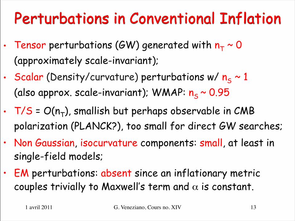
Perturbations in Conventional Inflation• Tensor perturbations (GW) generated with nT ~ 0

(approximately scale-invariant); • Scalar (Density/curvature) perturbations w/ nS ~ 1

(also approx. scale-invariant); WMAP: nS ~ 0.95

• T/S = O(nT), smallish but perhaps observable in CMB polarization (PLANCK?), too small for direct GW searches;

• Non Gaussian, isocurvature components: small, at least in single-field models;

• EM perturbations: absent since an inflationary metric couples trivially to Maxwell’s term and α is constant.

13

gµν = a2(η)(ηµν + hµν(η, �x)) ; ∂νhµν = hµµ = 0

h��k +

�k2 − a��

a

�hk = 0 ; hk = a(η)hk


Tensor perturbations in slow-roll inflationThis is one of the most robust predictions of inflation.Consider a tensor perturbation of the FLRW metric:

The associated “pump field” turns out to be a2(η) so that the Fourier modes of ah satisfy:

At early enough times the scale 1/k is inside the horizon. (ah) oscillates like exp(i k η) with constant amplitude. In the ground state of this harmonic oscillator QM gives:

hk = lP k−1/2 ⇒ δh(λ) = k3/2a−1hk =

lPλ

; λ = ak−1 ; lP =

�8πG�c2


At a later time the scale 1/k goes out of the horizon and h itself freezes. By matching the solution at exit we find:

hk = lP k−1/2 ⇒ δh(λ) = k3/2a−1hk =

lPλ

; λ = ak−1 ; lP =

�8πG�c2

Smaller wavelengths have a larger initial amplitude but they exit later and therefore are not amplified as much as longer wavelengths. These two competing effects produce a spectrum that depends on how H changes in time. For slow-roll inflation H(t) is a slowly decreasing function of t and therefore the resulting spectrum is expected to be slightly red-tilted. The amplitude is fixed in terms of H/MP.An almost scale-invariant (Harrison-Zel’dovich) spectrum of tensor perturbations from slow-roll inflation!

δh(λ) =lP

λ(ηex)∼ H(tex(λ))

MP; η > ηex


In slow-roll inflation this calculation can be repeated for “scalar” perturbations. These are coupled perturbations of the inflaton and of the metric (curvature perturbations).Because of this “mixing” the calculation is more complicated and one has to get rid of possible gauge artifacts.The end result is that also scalar perturbations have a flattish (and typically red-tilted) spectrum (ns ~ 1).Their amplitude is not fixed by H/MP since it is enhanced by 1/(slow-roll parameters). => The S contribution to CMB anisotropies dominates over T, but its properties are model-dependent.We can only put some upper bound on the tensor perturbations in order not to exceed the observed ΔT/T.Not clear whether PLANCK will see it in B-polarization...


Tensor Perturbations in string cosmologyUnlike in slow-roll inflation H is now rapidly varying in time:

=> we expect all but a flat spectrum of tensor perturbations

Since H grows in the pre-bang phase the spectrum is expected

to be blue-tilted (more power at short scales).

We have to find the “pump field” for tensor perturbations in

string cosmology. Because of the way the dilaton enters theeffective action one finds that the pump field is

P = exp(-φ/2) a = aE ~ η1/2

This implies nT = 3 (as opposed to nT = 0 in SRI)

=> possibly good for detection, irrelevant for CMB, LSS.17


atoti

tf

H-1

H-1

lP

tdec

18

λphys~ a(t)

exits

reentries

??

length scales

ls


recent LIGO/VIRGO bound

19


The reason why the spectrum is not flat in the stringy window is that we do not know the exact dynamics of the string phase. If H is constant but φ is not (e.g. has constant positive time derivative) the spectrum is blue-tilted.

A stochastic background of GW should be around us and can be detected, in principle, by looking for cross-correlations in two interferometers (in order to disentangle it from real noise).

Its discovery/measurement would give us a picture of the Universe when gravitons decoupled (like the CMB does for photons) i.e. of the Planck/string epoch, if it ever existed.

LIGO/VIRGO have recently lowered the upper bound on this stochastic background below the so-called NS bound (too many GW would have upset the successes of primordial nucleosynthesis, just like a 4th light neutrino).

20


Scalar perturbations in string cosmology

Like in ordinary inflation we can compute the spectrum of adiabatic curvature perturbations in string cosmology (coupled dilaton-metric perturbations).

Not surprisingly they also come out blue-tilted (ns = 4) and of the same order as tensor perturbations (no slow-roll enhancement of S/T in SC, in any case they are both tiny!)

Like with tensor perturbations this result is quite insensitive to what the extra dimensions do.

These perturbations are thus irrelevant for CMB, could be detectable in a narrow window of parameter space.

21


A problem with shear?

There is one potential problem with our scenario. It turns out that spatial isotropy is not necessarily an outcome of PBB evolution. The ratio:

σ/θ = (anisotropic expansion)/(total expansion)

is not diluted during dilaton-driven inflation (stays constant)

Isotropy appears to emerge instead from the stringy phase (similar to de Sitter) or could be a consequence of thermalization after the bounce.

In this connection: we have seen that Kasner-like behaviour was generic but isotropic Kasner was not.

22


Perturbations in string cosmology Gravitational waves: nT = 3

=> irrelevant for CMB, LSS, possibly good for detection

Adiabatic dilaton/curvature perturbations: nS = 4?

=> Irrelevant for CMB, LSS

• EM perturbations: amplified due to time-dependent φ, sensitive to evolution of internal space => Seeds for the dynamo of Cosmic Magnetic fields?

• Axionic perturbations are also amplified and their spectrum depends on the evolution of the extra dimensions in the pre-bounce phase. Can they be used for CMB, LSS?

23


The big question:Where does large scale structure come from?

24

Particules Élémentaires, Gravitation et Cosmologie Année ... · PDF...

Documents

Transcript of Particules Élémentaires, Gravitation et Cosmologie Année ... · PDF...