1

Tesista: Antonio Federico Zegarra BorreroAsesor: Dr. Carlos Javier Solano Salinas

“Particle Identification Algorithms for the Medium Energy

( 1.5-8 GeV)∼MINERνA Test Beam

Experiment”

UNI, March 04, 2016

2

Contents

● (1)The MINERνA Experiment at Fermilab● (2)Medium Energy MINERvA Test Beam experiment. ● (3)Tools for Data Analysis & Particle ID● (4)Results on the composition (% p ± , π ± , μ ± , e

±) of the secondary beam for different energies & polarities

● (5)Efficiency-Purity analysis to find the optimum cuts to separate different species for the 2GeV sample

● (6)Conclusions

3

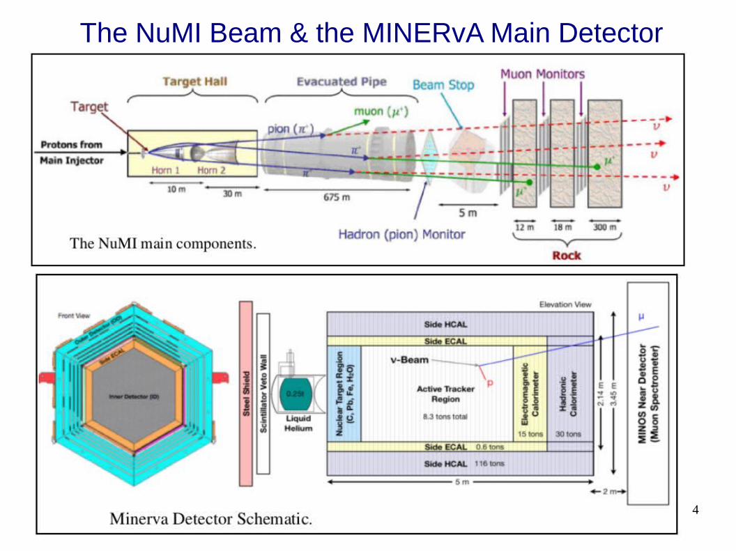
(1)The MINERνA Experiment at Fermilab

● Neutrino-Nucleon interactions & Neutrino Oscillation Experiments.

● Many Interaction-channels with different Cross-Sections at different Energies.

● Particles in the final state have a Specific-Pattern of depositing Energy inside the MINERνA main detector.

● Their Identification is important for the Reconstruction of the specific Event.

● Calculation of Cross-Sections.

4

The NuMI Beam & the MINERvA Main Detector

5

Data Acquisition (DAQ)

6

Energy Dependence of Neutrino Interactions

7

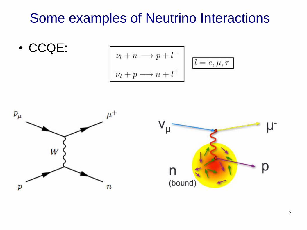
● CCQE:

Some examples of Neutrino Interactions

8

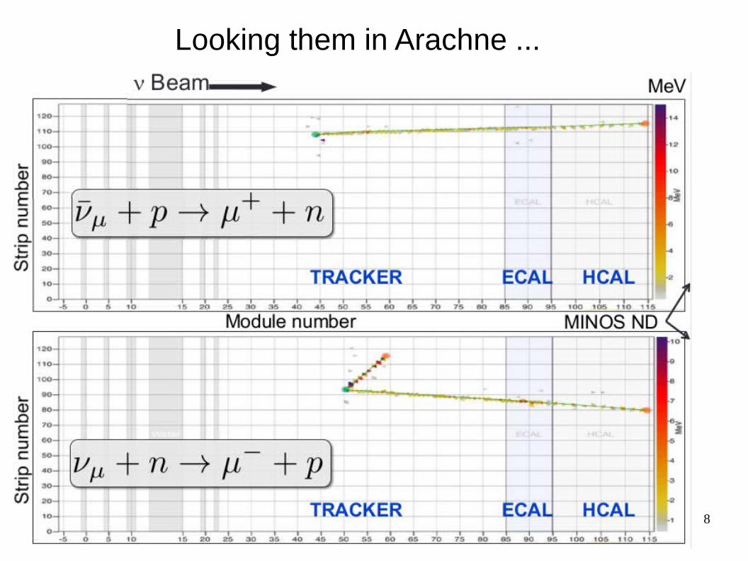
Looking them in Arachne ...

9

● RES production of a single π:

10

(2) Medium Energy MINERvA Test Beam experiment.

● Main Goal of the Medium Energy Test Beam experiment.

● Why ? ---> Test MC simulations

● How ? ---> Constructing up and analyzing a Beam

● Beamline elements:

11

12

Test Beam Detector Configurations

● Pion & Electron Data Samples (Folders)

● Advantage of the ECAL/HCAL configuration

● Different species –---> different behavior inside different Regions of the Detector (Energy deposition pattern, Number of Hits, etc...)

13

Time of Flight Device● Elements making up the 2 Stations (Upstream & DOWNstream)

● How this device separates different species (different masses)

● Interpretation of the ToF measured-time histogram

● Limitations (Resolution: at E > 8GeV & particles inside the Pion-peak)

14

● Early Result (ToF histogram) from its usage (Data from February 2015):

15

Limitations in the resolution of the ToF

● Resolution (ToF): 100-200 ps● Considering a momentum as low as 1 GeV/c:

● At E>= 8GeV other process (DIS) dominates neutrino-Int.

16

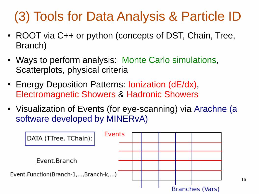
(3) Tools for Data Analysis & Particle ID● ROOT via C++ or python (concepts of DST, Chain, Tree,

Branch)

● Ways to perform analysis: Monte Carlo simulations, Scatterplots, physical criteria

● Energy Deposition Patterns: Ionization (dE/dx), Electromagnetic Showers & Hadronic Showers

● Visualization of Events (for eye-scanning) via Arachne (a software developed by MINERvA)

17

Interaction of particles with matter

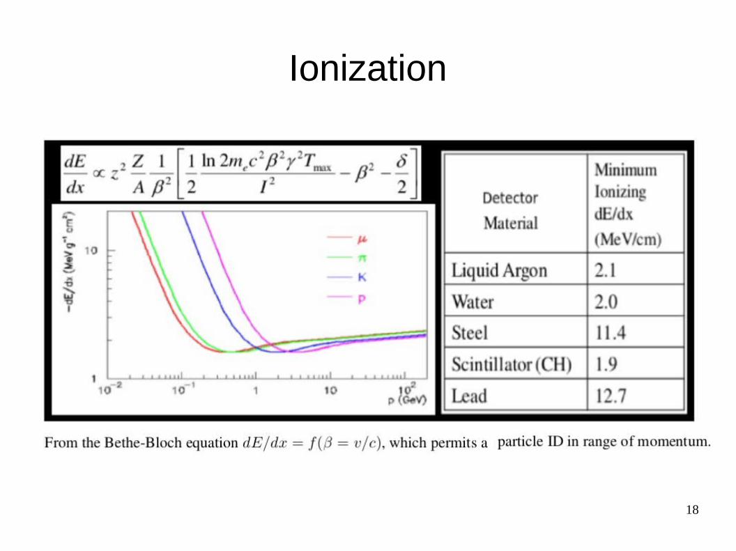
18

Ionization

19

Electromagnetic Showers

20

Hadronic Showers

21

Radiation & Interaction lengths in our Detector.

22

Tracks in the TB Detector seen in Arachne for a given view (XZ)

23

24

Mandatory Conditions to retain meaningful Events (==Particles)

● The Beam has to be ON:

● There is Activity in the Detector:

● All 6 PMTs of ToF Stations fire:

● The Veto does not fire:

● The Event occurs in the Triggered Slice:

● Relevant to know what Veto Branch to use (Veto Sanity Check) & an Analysis of Correlations between the ToF & the Veto

-----> 1 Event == 1 Particle ------> Start Isolating Species !

25

What is a Slice ?

26

Methodology for Particle Isolation

● In the ToF_measured_time histograms:– 1)Isolate the protons

– 2) Eye-Scanning Events in Contamination-Intervals

– 3)Isolate Events in the ToF Pion-peak (containing pions, muons & some electrons).

– 4)To Isolate Species inside the ToF Pion-peak (definition of Detector-Variables)

– For E >= 4GeV a cut in the histogram of Total-Energy deposited

– For the 2GeV sample we need to cut on more than 1 Variable !

27

● To separate Species (e, µ, π) inside the ToF π-peak:

– MC simulations of pure µ to find what Variable separates them better (µ are easier to locate).

– Definition of many Detector Variables to see which one works better (via python dictionaries of dE/dx, PE & Hits per module).

– How to look at any electron.

28

29

30

(4)Results on the composition (% p ± , π ± , μ ± , e ±) of the secondary beam for different energies &

polarities

● Methodology used for the 8 GeV π + sample (the same for the 4 & 6 GeV for both + & - polarities )

31

● Separating species in the ToF Pion-peak

32

● Patterns of Isolated species (from Data) & Pure species (Monte Carlo)

33

● The Relevant-Intervals in all histograms used for the isolation (in the ToF & Total-E) & how e+ are located (and counted) are detailed. The same criteria was used for the 6 & 4 GeV samples. Here Results for the 8GeV π+:

34

● Methodology used for the 2 GeV π + sample

-More than 1 Var to separate species in the Pion-peak

35

● For separating µ from π in the ToF Pion-peak– Not possible to rely on 1 single variable to separate µ from π

– 5 different kinds of cuts combining different variables

– The initial Logic was to look at π by knowing where µ are located

– These are the cuts that look at π (UNIONS) :

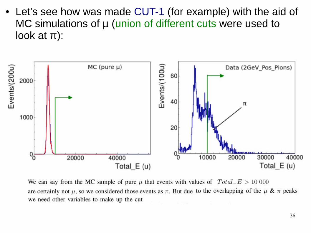
36

● Let's see how was made CUT-1 (for example) with the aid of MC simulations of µ (union of different cuts were used to look at π):

37

38

39

40

● So the particular cut called CUT-1 is a UNION of cuts of the Energy deposited in different regions of the detector & looks at π.

41

Results for All Energies & Polarities

● These results are estimations because there will never be perfect PID algorithms.

● For the 2GeV samples the specific CUT-i used are shown.

42

(5)Efficiency-Purity analysis to find the optimum cuts to separate different species

for the 2GeV sample● The Cuts used for the 2GeV samples: composed of a

UNION of cuts over different variables (5 per kind of Var).

● For Data Analysis: Reduce Number of Cuts –-> Reduce Systematic Uncertainties.

● The IDEA: construct an OPTIMUM-CUT composed of only 2 cuts (among the 20 Variables)

● For this reason an Efficiency-Purity Analysis was reliable

● To analyze each of the cuts & the effect of one after another –--> CHANGE IN THE LOGIC needed. This will look at µ instead of π

43

Change in the Logic to look at µ

44

For the MC an extra condition for the PE for the Hits for any Event was needed...

45

The Analysis began while looking for the Best Variable to separate µ from π …

46

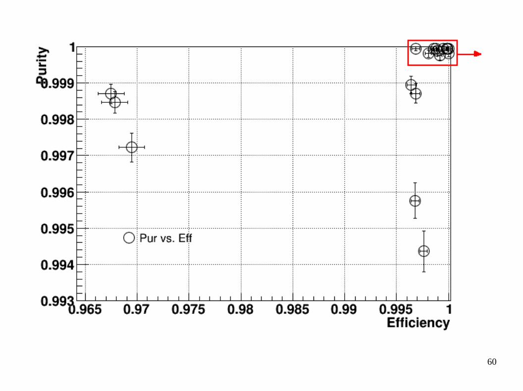
Concepts of Efficiency & Purity

47

48

49

50

● Best cuts to separate µ from π. Plot histograms of other Vars for events in the µ-interval (for the best cut) –---> To find the Best second cut.

51

Methodology followed

● Select the Best-Cut (let's call it in Variable ) to retain Events in the µ-Interval ( ).

● Fill histograms of the other variables with the previous Events to see which variable (let's call it ) separates better the µ & π present there. Select remaining µ in the new µ-interval ( ) of this new histogram.

● 8 candidates were selected as the second cut (to add to the one cited above) and the most efficient (in selecting µ) among them was chosen.

52

New-Logic of the “Cuts”:

● Cut_µ =={ }

● Cut_π ==

(*)=={ } == ~ Cut_µ

● Applying these cuts to the MC samples of pure µ & π we can find the efficiencies:

– Fraction of µ looking as µ(pass the Cut_µ):

– Fraction of µ looking as π:

– The same for the case of π:

● The best cut was chosen as the one which maximizes

53

Candidate to be the Var

54

● In next slides: histograms of the variable (8 candidates) for events in which

● For each case: new µ-interval is shown, together with the four numbers:

● The 8 candidates for are:

– Total_E– Total_E_HCAL– Total_PE– Total_PE_HCAL– <dE/dx>_Total– <dE/dx>_HCAL– Total_Hits_HCAL– Total_Hits_L8P

55

● Due to its highest efficiency, the 2nd variable was chosen to be Total_PE_HCAL

56

57

Application (of this cut == composition of 2 cuts) to Data

● Relations :

58

A similar procedure for the Cut (only 1 cut in variables of type

Var_i_ß is enough) that separate e from µ : (Here just results of the

best cuts found)

59

Type of cut refers to any of the 20 sub-cuts to separate e from µ

60

61

62

Some notes about e-µ separation● Many good cuts to separate e from µ.

● Many cuts in LP-Vars are almost perfect. We expect that electrons will almost never arrive at the LP so this is physically expected.

● I believe that the best-cut (Hits_L8P) is enough for a very good separation.

● The best cuts to separate any e that may be in a µ sample would be the ones with highest values of Eff*Pur:

63

& for the Cut (again an intersection of 2 cuts ) to

separate e from π …

64

The Procedure for the PID would be

● Considering that:

*Cut_i_j= Cut to separate species “i” from “j”

*Cut_j_i = ~ Cut_i_j

● & that the cuts “Cut_i_j” are already known:

● ===> the way to do PID for π & e Folders of DR1 is:

65

The way to apply the Tool

66

(6)Conclusions

● Estimations on the Composition of the Secondary Beam as well as Efficient Tools for the Identification of specific kinds of particle species.

● Importance: For MINERvA (To PID particles in its ECAL/HCAL region in order to reconstruct Events), the Test Beam (to test the efficiency of its beamline elements), the Accelerator Division & for comparisons with a MC simulation of the secondary beam (in progress).

● The usage of the variables Var_i_ß have proven to be useful and agreed with the physical expectations.

● There will not be perfect PID algorithms

● The Efficiency-Purity analysis permits to look at any kind of particle species that we think may be present in the secondary beam

● The importance of my work is to show estimations and a specific way to proceed in order to make up the Tool for particle isolation, since Data is not full calibrated yet.