Particle Filter Theory and Practice with Positioning …360880/FULLTEXT… · ·...

Linköping University Post Print

Particle Filter Theory and Practice with

Positioning Applications

Fredrik Gustafsson

N.B.: When citing this work, cite the original article.

©2010 IEEE. Personal use of this material is permitted. However, permission to

reprint/republish this material for advertising or promotional purposes or for creating new

collective works for resale or redistribution to servers or lists, or to reuse any copyrighted

component of this work in other works must be obtained from the IEEE.

Fredrik Gustafsson , Particle Filter Theory and Practice with Positioning Applications, 2010,

IEEE AEROSPACE AND ELECTRONIC SYSTEMS MAGAZINE, (25), 7, 53-81.

http://dx.doi.org/10.1109/MAES.2010.5546308

Postprint available at: Linköping University Electronic Press

http://urn.kb.se/resolve?urn=urn:nbn:se:liu:diva-61199

http://dx.doi.org/10.1109/MAES.2010.5546308

http://urn.kb.se/resolve?urn=urn:nbn:se:liu:diva-61199

Particle Filter Theory and Practice with Positioning Applications

FREDRIK GUSTAFSSON, Senior Member, IEEE Linkoping University Sweden

The particle filter (PF) was introduced in 1993 as a numerical

approximation to the nonlinear Bayesian filtering problem, and

there is today a rather mature theory as well as a number of

successful applications described in literature. This tutorial

serves two purposes: to survey the part of the theory that is most

important for applications and to survey a number of illustrative

positioning applications from which conclusions relevant for the

theory can be drawn.

The theory part first surveys the nonlinear filtering problem

and then describes the general PF algorithm in relation to

classical solutions based on the extended Kalman filter (EKF) and

the point mass filter (PMF). 'TIming options, design alternatives,

and user guidelines are described, and potential computational

bottlenecks are identified and remedies suggested. Finally, the

marginalized (or Rao-Blackwellized) PF is overviewed as a

general framework for applying the PF to complex systems.

The application part is more or less a stand-alone tutorial

without equations that does not require any background

knowledge in statistics or nonlinear filtering. It describes a

number of related positioning applications where geographical

information systems provide a nonlinear measurement and where

it should be obvious that classical approaches based on Kalman

filters (KFs) would have poor performance. All applications are

based on real data and several of them come from real-time

implementations. This part also provides complete code examples.

Manuscript received June 18 , 2008 ; revised January 26 and June 17 , 2009; released for publication September 8, 2009.

Refereeing of this contribution was handled by L. Kaplan.

Author's address : Dept. of Electrical Engineering, Linkoping University, ISY, Linkoping, SE-58l83, Sweden, E-mail: ([email protected]).

0018-925 1 110/$1 7 .00 © 20 10 IEEE

I . I NTROD U CTION

A dynamic system can in general terms be characterized by a state-space model with a hidden state from which partial information is obtained by observations. For the applications in mind, the state vector may include position, velocity, and acceleration of a moving platform, and the observations may come from either internal onboard sensors (the navigation problem) measuring inertial motion or absolute position relative to some landmark or from external sensors (the tracking problem) measuring for instance range and bearing to the target.

The nonlinear filtering problem is to make inference on the state from the observations. In the Bayesian framework, this is done by computing or approximating the posterior distribution for the state vector given all avai lable observations at that time. F or the applications in mind, this means that the position of the platform is represented with a conditional probability density function (pdf) given the observations.

Classical approaches to Bayesian nonlinear filtering described in literature include the following algorithms:

1 ) The Kalman filter (KF ) [l, 2] computes the posterior distribution exact ly for linear Gaussian systems by updating finite-dimensional stati stics recursively.

2) F or nonlinear, non-Gaussian models, the KF algorithm can be applied to a linearized model with Gaussian noi se with the same fir st- and second-order moments. This approach is commonly referred to as the extended Kalman filter (E KF ) [3,4]. This may work well but without any guar antees for mildly nonlinear systems where the true posterior is unimodal Gust one peak) and essentially symmetric.

3) The unscented Kalman filter (UKF ) [5,6] propagates a number of point s in the state space from which a Gaussian distribution is fit at each time step. UKF is known to accomodate also the quadratic term in nonlinear models, and is often more accurate than EKF. The divided difference filter (DDF ) [7] and the quadrature Kalman filter (QKF ) [8] are two other variants of this principle. Again, the applicability of these filters i s limited to unimodal posterior distributions.

4) Gaussian sum Kalman filters (GS-KFs) [9] represent the posterior with a Gaussian mixture distribution. Filters in this class can handle multimodal posteriors. The idea can be extended to KF approximations like the GS-Q KF in [8].

5) The point mass filter (PMF ) [ 10, 9] grids the state space and computes the posterior over this grid recursively. PMF applies to any nonlinear and non-Gaussi an model and is able to represent any posterior distribution. The main limiting factor is the curse of dimensionality of the grid size in higher state

IEEE A&E SYSTEMS MAGAZINE VOL. 25, NO. 7 JULY 201 0 PART 2: TUTORlALS-GUSTAFSSON 53

-+-PForSMC - PF or SMC and application -+- Citations to Gor<lon

2000

1500

1000

500

1996 1998 2000 2002 2004 2006 2008 Year

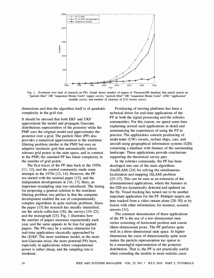
Fig. 1 . Evolution over time of research on PFs. Graph shows number of papers in Thomson/ISI database that match search on "particle filter" OR "sequential Monte Carlo" (upper curve), "particle filter" OR "sequential Monte Carlo" AND "application"

(middle curve), and number of citations of [ 15 ] (lower curve) .

dimensions and that the algorithm itself is of quadratic complexity in the grid size.

It should be stressed that both EKF and UKF approximate the model and propagate Gaussian distributions representitive of the posterior while the PMF uses the original model and approximates the posterior over a grid. The particle filter (PF) also provides a numerical approximation to the nonlinear filtering problem similar to the PMF but uses an adaptive stochastic grid that automatically selects relevant grid points in the state space, and in contrast to the PMF, the standard PF has linear complexity in the number of grid points.

The first traces of the PF date back to the 1950s [11 , 12] , and the control community made some attempts in the 1970s [ 13 , 14]. However, the PF era started with the seminal paper [ 15] , and the independent developments in [ 16 , 17]. Here, an important resampling step was introduced. The timing for proposing a general solution to the nonlinear filtering problem was perfect in that the computer development enabled the use of computationally complex algorithms in quite realistic problems. Since the paper [ 15] the research has steadily intensified; see the article collection [ 18] , the surveys [ 19-22] , and the monograph [23]. Fig. I i llustrates how the number of papers increases exponentially each y ear, and the same appears to be true for applied papers. The PFs may be a serious alternative for real-time applications classically approached by the (E)KF. The more nonlinear model, or the more non-Gaussian noise, the more potential PFs have, especially in applications where computational power is rather cheap, and the sampling rate i s moderate.

Positioning of moving platforms has been a technical driver for real-time applications of the PF in both the signal processing and the robotics communities. F or this reason, we spend some time explaining several such applications in detail and summarizing the experiences of using the PF in practice. The applications concern positioning of underwater (UW) vessels , surface ships , cars , and aircraft using geographical information systems (GIS) containing a database with features of the surrounding landscape. These applications provide conclusions supporting the theoretical survey part.

In the robotics community, the PF has been developed into one of the main algorithms (fastS LAM) [24] for solving the simultaneous localization and mapping (SLAM) problem [25-27]. This can be seen as an extension of the aforementioned applications , where the features in the GIS are dynamically detected and updated on the fly. Visual tracki ng has turned out to be another important application for the PF. MUltiple targets are here tracked from a video stream alone [28-30] or by fusion with other information, for instance, acoustic sensor s [3 1].

The common denominator of these applicat ions of the PF is the use of a low-dimensional state vector consisting of horizontal position and course (three-dimensional pose). The PF performs quite well in a three-dimensional state space. In higher dimensions the curse of dimensionality quite soon makes the particle representation too sparse to be a meaningful representation of the posterior distribution. That is , the PF is not practically useful when extending the models to more realistic cases

5 4 IEEE A&E SYSTEMS MAGAZINE VOL. 25, NO. 7 JULY 20 10 PART 2: TUTORIALS

with

1) motion in three dimensions (six-dimensional pose) ,

2) more dynamic states (accelerations , unmeasured velocities , etc.) ,

3) or sensor biases and drifts.

A technical enabler for such applications is the margin alized PF (MPF), also referred to as the Rao-Blackwellized PF (RBPF). It allows for the use of high-dimensional state-space models as long as the (severe) nonlinearities only affect a small subset of the states. In this way the structure of the model is utilized so that the particle filter is used to solve the most difficult tasks , and the (E)KF is used for the (almost) linear Gaussian states. The fastS LAM algorithm is in fact a version of the MPF, where hundreds or thousands of feature points in the state vector are updated using the (E)KF. The need for the MPF in the list of applications will be motivated by examples and experience from practice.

This tutorial uses notation and terminology that should be familiar to the AES community, and it deliberately avoids excessive use of concepts from probability theory, where the main tools here are Bayes' theorem and the marginalization formula (or law of total probability). There are explicit comparisons and references to the KF, and the applications are in the area of target tracking and navigation. For instance, a particle represents a (target ) state trajectory; the (target) motion dynamics and sensor observation model are assumed to be in state-space form, and the PF algorithm is split into time and measurement updates.

The PF should be the nonlinear filtering algorithm that appeals to engineers the most since it intimately addresses the system model. The filtering code is thus very similar to the simulation code that the engineer working with the application should already be quite familiar with. F or that reason, one can have a code-first approach, starting with Section IX to get a complete simulation code for a concrete example. This section also provides some other exam ples using an object-oriented programming framework where models and signals are represented with objects , and can be used to quickly compare different filters , tunings , and models. Section X provides an overview of a number of applications of the PF, which can also be read stand-alone. Section XI extends the applications to models of high s tate dimensions where the MPF has been applied. The practical experiences are summarized in Section XII.

H owever, the natural structure is to start with an overvi ew of the PF theory as found in Section I I , and a summary of the MPF theory is provided in Section VIII , where the selection of topics is strongly influenced by the practical experiences in Section XII.

I I . N O N L I N EAR FI LTE R I N G

A. Models a n d Notation

Applied nonlinear filtering is based on discrete time nonlinear state-space models relating a hidden state xk to the observations Yk:

xk+l = f(xk' vk)' vk rv PVk' Xl rv PX] ( 1 a)

( 1b)

Here k denotes the sample number, vk is a stochastic noise process specified by its known pdf Pv ' which is compactly expressed as vk rv PVk. Similarly ek is an additive measurement noise also with known pdf P e •

The first observation is denoted Yl' and thus the fir;t unknown state is Xl where the pdf of the initial state is denoted Px . The model can also depend on a known (control) idput Uk' so f(xk,uk, vk) and h(xk , uk) , but this dependence is omitted to simplify notation. The notation sl:k denotes the sequence sl, s2 , . . . , sk (s is one of the signals x, v , y ,e) , and ns denotes the dimension of that signal.

In the statistical literature, a general Markov model and observation model in terms of conditional pdfs are often used

(2a)

(2b)

This is in a sense a more general model. For instance, (2) allows implicit measurement relations h(Yk ,xk ,ek) = 0 in (1b) , and differential algebraic equations that add implicit state constraints to ( 1a).

The B ayesian approach to nonlinear filtering is to compute or approximate the posterior distribution for the state given the observations. The posterior is denoted p(xk I Yl:k) for filtering, p(xk+m I Yl:k) for prediction, and p(xk-m I Yl:k) for smoothing where m > 0 denotes the prediction or smoothing lag. The theoretical derivations are based on the general model (2) , while algorithms and discussions are based on (1). Note that the Markov property of the model (2) implies the formulas P(xk+l I xl:k , Yi:k) = P(xk+l I xk) and P(Yk I Xl:k'YI:k-l) = P(Yk I xk) , which are used frequently.

A linearized model will tum up on several occasions and is obtained by a first-order Taylor expansion of ( 1) around xk = xk and vk = 0:

xk+l = f(xk , 0) + F (xk)(xk - xk) + G(xk)vk (3a)

(3b)

where

IEEE A&E SYSTEMS MAGAZINE VOL. 25, NO. 7 JULY 20 10 PART 2: TUTORIALS-GUSTAFSSON 55

and the noise is represented by their second-order moments

COV(Xl) = Po.

(3d)

F or instance, the EKF recursions are obtained by linearizing around the previous estimate and applying the KF equations , which gives

Kk = ltlk_lHT(Xklk_l) A TA l

x (H(Xklk-l)ltlk-IH (Xklk-l) + Rk)- (4a)

Xklk = Xklk-l + Kk(Yk -hk(Xklk-I» (4b)

ltlk = ltlk-l -KkH(Xklk-l)ltlk-1 (4c)

Xk+llk = f(Xklk' 0) (4d)

It+llk = F (Xklk)ltlkFT (Xklk) + G(Xklk)QGT (Xklk) ' (4e)

The recursion is initialized with xllo = Xo and lilo = Po, assuming the prior p(xl) '" N(xo' Po)· The EKF approximation of the posterior filtering distribut ion is then

(5)

where N(m,P) denotes the Gaussian density function with mean m and covariance P. The special case of a linear model is covered by (3) in which case F (xk) = Ft, G(xk) = Gk, H(xk) = Hk; using these and the equalities f(xk'O) = Fkxk and h(xk) = Hkxk in (4) gives the standard KF recursion.

The neglected higher order terms in the Taylor expansion imply that the EKF can be biased and that it tends to underestimate the covariance of the state estimate. There is a variant of the EKF that also takes the second-order term of the Taylor expansion into account [32]. This is done by adding the expected value of the second-order term to the state updates and its covariance to the state covariance updates. The UKF [5, 6] does a similar correction by using propagation of systematically chosen state points (called s igma points) through the model. Related approaches include the DDF [7] that uses Sterling's formula to find the sigma points and the QKF [8] that uses the quadrature rule in numerical integration to select the sigma points. The common theme in EKF, UKF, DDF, and QKF is that the nonlinear model is evaluated in the current state estimate. The latter filters have some extra points in common that depend on the current state covariance.

UKF is closely related to the second-order EKF [33]. Both variants perform better than the EKF in certain problems and can work well as long as the posterior distribution is unimodal. The algorithms are prone to diverge, a problem that is hard to mitigate or foresee by analytical methods. The choice of state

coordinates is therefore crucial in EKF and UKF (see [34 , ch. 8.9.3] for one example) while this choice does not affect the performance of the PF (more than potential numerical problems).

B. Bayesian Fi lter ing

T he Bayesian solution to computing the posterior distribution P(xk I Yl:k ) of the state vector, given past observations , is given by the general Bayesian update recursion:

( I ) - P(Yk I xk)P(xk I Yl:k-l) P xk Yl:k - P(Yk I Yl:k-l) (6a)

(6c)

This classical result [35 , 36] is the cornerstone in nonlinear Bayesian filtering. The first equation follows directly from Bayes' law, and the other two follow from the law of total probability, using the model (2). T he first equation corresponds to a measurement update, the second is a normalization constant , and the third corresponds to a time update.

T he posterior distribution is the primary output from a nonlinear filter, from which standard measures as the minimum mean square (MMS) est imate xrMS and its covariance IktrS can be extracted and

compared with EKF and UKF outputs:

XWS = J xkP(xk I Yl:k )dxk (7a)

RMMS - J( AMMS)( AMMS)T ( I )d klk - Xk - Xk Xk -Xk P Xk Yl:k Xk· (7b)

F or a linear Gaussian model, the KF recursions in (4) also provide the solut ion (7) to this Bay esian problem. However, for nonlinear or non-Gaussian models there is in general no finite-dimensional representation of the posterior distribut ions similar to (XWs ,1k�MS). That is why numerical approximations are needed.

C. The Poi nt Mass Fi lter

Suppose now we have a deterministic grid {xi}f:l of the state space Rnx over N points , and that at time k, bas ed on observations Yl:k-l' we have computed the relat ive probabilites (assuming distinct grid points)

(8)

satisfying ��l W�lk-l = 1 (note that this is a relative normalization with respect to the grid points). The notation x� is introduced here to unify notation with the PF, and it means that the state xk at t ime k visits

56 IEEE A&E SYSTEMS MAGAZINE VOL. 25 , NO. 7 JULY 20 10 PART 2: TUTORIALS

the grid point Xi. The predict ion density and the ftrst two moments can then be approximated by

N P(Xk I Yl:k-l) = Lwilk-lO(Xk - xi) i=l

N xklk-l = E(Xk) = Lwilk-lxi

lllk-l = cOV(Xk) N

i=l

(9a)

(9b)

= L Wilk-l (xi - xklk-l ) (xi - xklk_1 )T. i=l

Here , o(x) denotes the Dirac impulse function. The Bayesian recursion (6) now gives

N P(xk I Yl:k) = L: P(Yk I xi)wilk-l O(xk - xi) i=l , k , 'V

(9c)

N ck = LP(Yk I xi)wilk-l

(10a)

(lOb) i=l N

P(xk+l I Yl:k) = LwilkP(Xk+l I xi)· (10c) i= l

Note t hat the recursion starts with a discrete approximation (9a) and ends in a continuous distribution (lOc). Now, to close the recursion, the standard approach is to sample (lOc) at the grid points Xi, which computationally can be seen as a multidimensional convolution,

N Wi+llk = P(Xi+l I YI:k) = Lw{lkP(xi+l l.xfc),

j=l i = 1 , 2, . . . ,N . (11)

This is the principle of the PMF [9 , 10] , whose advantage is its simple implementat ion and tuning (the engineer basically only has to consider the size and resolution of the grid). The curse of dimensionality limits the application of PMF to small models (nx less than two or three) for two reasons: the ftrst one is that a grid is an inefficiently sparse representat ion in higher dimensions , and the second one is that the multidimensional convolution becomes a real bottleneck with quadratic complexity in N . Another practically important but difficult problem is to translate and change the resolution of the grid adaptively.

I I I . THE PARTICLE FI LTER

A. R elation to the Poi nt Mass Fi lter

The PF has much in common with the PMF. Both algorithms approximate the posterior distribution with

a discrete density of the form (9a), and they are both b ased on a direct applicat ion of (6) leading to the numerical recursion in (10). However, there are some major differences:

I) The deterministic grid xi in the PMF is replaced with a dynamic stochastic grid xi in the PF that changes over time. The stochastic grid is a much more efftcient representation of the state space than a ftxed or adaptive deterministic grid in most cases.

2) The PF aims at estimating the whole trajectory

x\:k rather than the current state xk. That is , the PF generates and evaluates a set {xLk}f: 1 of N different trajectories. This affects (6c) as follows:

P(�:k+l I Yl:k) = P(Xi+l I xLk'Yl:k) P(xLk I Yl:k) , ... '� p(.xi+ [ Ixi) W�lk

(12) = WilkP(xi+l I x�). (13)

Comparing this to (lOc) and (11) , we note th at the double sum leading to a quadratic complexity is avoided by this trick. However, this quadratic complexity appears if one wants to recover the marginal distribution P(xk I Yl:k) from p(x\:k I Yl:k)' more on this in Section I I IC.

3) The new grid in the PF is obtained by sampling from (lOc) rather than reusing the old grid as done in the PMF. The original version of the PF [15] samples from (lOc) as it stands by drawing one sample each from p(xk+ 1 I xi) for i = 1 , 2, . . . , N . More generally, the concept of importance sampling [37] can be used. The idea is to introduce a proposal density

q(xk+1 I xk'Yk+l)' which is easy to sample from, and rewrite (6c) as

P(xk+1 I Yl:k) = r P(xk+l I xk)P(xk I Yl:k)dxk iIRnx l ( I ) P(xk+l I xk) = q xk+l xk'Yk+l ( I ) JRn, q xk+l xk'Yk+l X p(xk I Yl:k)dxk. (14)

The trick now is to generate a sample at random from

x�+l ,....., q(xk+l I Xi,Yk+l) for each particle , and then adjust the posterior probability for each part icle with the importance weight

As indicated, the proposal distribution q(�+l I xi'Yk+l) depends on the last state in the particle trajectory .xi:k' but also the next measurement Yk+l. The simplest choice of proposal is to use the dynamic model itself q(x�+l I x�'Yk+l) = P(�+l I xD leading to Wi+llk = Wilk. The choice of proposal and its actual form are

discussed more thoroughly in Sect ion V.


4) Resampling is a crucial step in the PF. Without resampling, the PF would break down to a set of independent simulations yielding trajectories

xLk with relative probabilities wi. Since there would then be no feedback mechanism from the observations to control the simulations, they would quite soon diverge. As a result, all relative weights would tend to zero except for one that tends to one. This is called sample depletion, sample degeneracy, or sample impoverishment. Note that a relative weight of one Wilk � 1 is not at all an indicator of how close a trajectory is to the true trajectory since this is only a relative weight. It merely says that one sequence in the set {xLk};:1 is much more likely than all of the other ones. Resampling introduces the required information feedback from the observations, so trajectories that perform well will survive the resampling. There are some degrees of freedom in the choice of resampling strategy discussed in Section IVA.

B. Algorithm

The PF algorithm is summarized in Algorithm 1 . It can be seen as an algorithmic framework from which particular versions of the PF can be defined later on. It should be noted that the most common form of the algorithm combines the weight updates ( 1 6a, d) into one equation. Here, we want to stress the relations to the fundamental Bayesian recursion by keeping the structure of a measurement update (6a)-( 10a)-( 16a), normalization (6b)-( 10b)-( 1 6b), and time update (6c)-( 10c)-( 16c, d).

ALGORITHM 1 Particle Filter Choose a proposal distribution q(xk+1 I xI:k'Yk+I)' resampling strategy, and the number of particles N.

Initialization: Generate x; f'V PXo' i = 1 , . . . , N and let wilo = liN.

Iteration For k = 1 , 2, . . . . 1 ) Measurement update: For i = 1 , 2, . . . , N,

i _I i (y I i) Wklk - -wklk-1P k Xk ck where the normalization weight is given by

N

ck = L Wilk-IP(Yk I xi)· i=1

( 1 6a)

( 1 6b)

2) Estimation: The filtering density is approximated A N · .

by p(xl:k I Yl:k) = Li=1 wk1k8(xl:k - x'l:k) and the mean

(7a) is approximated by xl:k � L;:'I wilkxLk' 3) Resampling: Optionally at each time, take

N samples with replacement from the set {xLk};:1 where the probability to take sample i is wklk and let

wilk = liN.

4) Time update: Generate predictions according to the proposal distribution

xi+ 1 f'V q(xk+1 I Xi,Yk+I) and compensate for the importance weight

i _ i p(xi+ 1 I xD wk+llk - wklk q(� I Xi Y ) ' k+1 k' k+1

C. Pred iction, Smoothi ng, and Margi nals

( 1 6c)

( 1 6d)

Algorithm 1 outputs an approximation of the trajectory posterior density p(xl:k I YI:k) ' For a filtering problem, the simplest engineering solution is to just extract the last state xi from the trajectory A:k and use the particle approximation

N

p(xk I YI:k) = L Wilk8(Xk - xi)· ( 1 7) i=1

Technically this is incorrect, and one may overlook the depletion problem by using this approximation. The problem is that in general all paths x{:k-I can lead to the state x� . Note that the marginal distribution is functionally of the same form as (6c) . The correct solution taking into account all paths leading to x� leads (similar to ( 1 1 )) to an importance weight

N . . .

i Lj=1 �lkP(x'k+ 1 I xi) wk+llk = i i ( 1 8) q(xk+1 I xk'Yk+l) that replaces the one in ( 1 6d) . That is, the marginal PF can be implemented just like Algorithm 1 by replacing the time update of the weights with ( 1 8) . Note that the complexity increases from O(N) in the PF to O(N2) in the marginal PF, due to the new importance weight. A method with O(N log(N)) complexity is suggested in [38] .

The marginal PF has found very interesting applications in system identification, where a gradient search for unknown parameters in the model is applied [39, 40] . The same parametric approach has been suggested for SLAM in [4 1 ] and optimal trajectory planning in [42] .

Though the PF appears to solve the smoothing problem for free, the inherent depletion problem of the history complicates the task, since the number of surviving trajectories with a time lag will quickly be depleted. For fixed-lag smoothing p(xk-m:k I Yl:k)' one can compute the same kind of marginal distributions as for the marginal PF leading to another compensation factor of the importance weight. However, the complexity will then be O(Nm+ 1 ) . Similar to the KF smoothing problem, the suggested solution [43] is based on first running the PF in the usual way and then applying a backward sweep of a modified PF.

58 IEEE A&E SYSTEMS MAGAZINE VOL. 25 , NO. 7 JULY 20 10 PART 2: TUTORIALS

The prediction to get P(Xl:k+m I Yl:k) can be implem ented by repeating the time update in Algorithm 1 m times .

D. Read i ng Advice

The reader may at this stage continue to Section IX to see MATLAB ™ code for some illustrative examples , or to Section X to read about the results and experiences using some other applicat ions , or proceed to the subsequent sections that discuss the following issues:

1 ) The tuning possibilities and different versions of the b asic PF are discussed in Section IV.

2) The choice of proposal distribution is crucial for performance, just as in any classical sampling algorithm [ 37] , and this is discussed in Section V.

3) Performance in terms of convergence of the approximation p(X\:k I Yl:k) ---7 p(x\:k I Y\:k) as N ---7 00 and relat ion to fundamental performance bounds are discussed in Section VI .

4) The PF is computat ionally quite complex , and some potential bottlenecks and possible remedies are discussed in Section VII.

IV. TUN I NG

The number of particles N is the most immediate design parameter in the PE There are a few other degrees of freedom discussed below. The overall goal is to avoid sample depletion, which means that only a few particles , or even only one, contribute to the state estimate. The choice of proposal distribution is the most intricate one, and it is discussed separately in Section V. How the resampling strategy affects sample deplet ion is discussed in Sect ion IVA. The effective number of samples in Sect ion IVB is an indicator of sample deplet ion in that it measures how efficiently the PF is utilizing its particles . It can be used to design proposal distributions , depletion mitigation tricks , and resampling algorithms and also to choose the number of particles . It can also be used as an online control variable for when to resample. Some dedicated tricks are discussed in Sect ion Ive .

A. Resampl i ng

Without the resampling step, the basic PF would suffer from sample deplet ion. This means that after a while all particles but a few will have negligible weights . Resampling solves this problem but creates another in that resampling inevitably destroys information and thus increases uncertainty in the random sampling. It is therefore of interest to start the resampling process only when it is really needed. The following options for when to res ample are possible.

1) The standard version of Algorithm 1 is termed sampling importance resampling (SIR), or bootstrap PF, and is obtained by resampling each time.

2) The alternative is to use importance sampling, in which case resampling is performed only when needed. This is called sampling importance sampling (SIS) . Usually, resampling is done when the effective number of samples , as will be defined in the next section, becomes too small.

As an alternative, the res amp ling step can be replaced with a sampling step from a distribution that is fitted to the particles after both the t ime and measurement update. The Gaussian PF (GPF ) in [44] fits a Gaussian distribution to the particle cloud after which a new set of part icles is generated from this distribution. The Gaussian sum PF (GSPF ) in [45] uses a Gaussian sum instead of a distribution.

B. Effective N u m ber of Samples

An indicator of the degree of depletion is the effective number of samples ,l defined in terms of the coefficient of variation Cv [ 1 9, 46, 47] as

N - N = N =

N eff -1 + c�(w1Ik) Var(w1Ik) 1 + N2Var(w1Ik) ·

1 + . 2 (E(wk1k» (19a)

The effective number of samples is thus at its maximum Neff = N when all weights are equal W�lk = liN, and the lowest value it can attain is Neff = 1 , which occurs when w�lk = 1 with probability liN and

w�lk = 0 with probability (N - l)IN. A logical computable approximation of Neff is

provided by

(l9b )

This approximation shares the property 1 :::; !jeff :::; N with the definit ion (l9a) . The upper bound Neff = N is attained when all particles have the same weight and

the lower bound Neff = 1 when all the probability mass is devoted to a single particle.

The res�pling condition in the PF can now be

defined as Neff < Nth . The threshold can for instance be

chosen as Nth = 2N 1 3.

C. Tricks to Mitigate Sample Depletion

The choice of proposal distribution and resampling strategy are the two available instruments to avoid sample deplet ion problems . There are also some simple and more practical ad hoc tricks that can be tried as discussed below.

I Note that the literature often defines the effective number of samples as N /0 + Var(wk

lk»' which is incorrect.


One important trick is to modify the noise models so the state noise and/or the measurement noise appear larger in the filter than they really are in the data generating process. This technique is called "jittering" in [48] , and a similar approach was introduced in [ 1 5] under the name "roughening." Increasing the noise level in the state model ( la) increases the support of the sampled particles, which partly mitigates the depletion problem. Further, increasing the noise level in the observation model ( 1b) implies that the likelihood decays slower for particles that do not fit the observation, and the chance to resample these increases. In [49] , the depletion problem is handled by introducing an additional Markov Chain Monte Carlo (MCMC) step to separate the samples.

In [ 1 5] , the so-called prior editing method is discussed. The estimation problem is delayed one time step so that the likelihood can be evaluated at the next time step. The idea is to reject particles with sufficiently small likelihood values, since they are not likely to be resampled. The update step is repeated until a feasible likelihood value is received. The roughening method could also be applied before the update step is invoked. The auxiliary PF [50] is a more formal way to sample such that only particles associated with large predictive likelihoods are considered; see Section VF.

Another technique is regularization. The basic idea to is convolve each particle with a diffusion kernel with a certain bandwidth before resampling. This will prevent multiple copies of a few particles. One may for instance use a Gaussian kernel where the variance acts as the bandwidth. One problem in theory with this approach is that this kernel will increase the variance of the posterior distribution.

V. CHOICE OF PROPOSAL D I STRI BUTION

In this section we focus on the choice of proposal distribution, which influences the depletion problem significantly, and we outline available options with some comments on when they are suitable.

First note that the most general proposal distribution has the form q(x\:k 1 Y\:k). This means that the whole trajectory should be sampled at each iteration, which is clearly not attractive in real-time applications. Now, the general proposal can be factorized as

(20)

The most common approximation in applications is to reuse the path x\:k_1 and only sample the new state xk , so the proposal q(xI:k 1 Y\:k) is replaced by q(xk 1 x\:k_1 'YI:k)· The approximate proposal suggests good values of xk only, not of the trajectory x\:k.

For filtering problems this is not an issue, but for smoothing problems the second factor becomes important. Here, the idea of block sampling [5 1 ] is quite interesting.

Now, due to the Markov property of the model, the proposal q(xk 1 X\:k_1 'Y\:k) can be written as

q(xk 1 xl:k-I'Y\:k) = q(xk 1 xk-l'Yk)· (2 1 )

The following sections discuss various approximations of this proposal and in particular how the choice of proposal depends on the signal-to-noise ratio (SNR). For linear Gaussian models, the SNR is in loose terms defined as I IQI I/ I IRI I; that is, the SNR is high if the measurement noise is small compared with the signal noise. Here, we define SNR as the ratio of the maximal value of the likelihood to the prior,

SNR ex maxXk P(Yk 1 xk) . maxxkP(xk 1 xk-l)

For a linear Gaussian model, this gives SNR ex Jdet(Q)1 deteR). In this section we use the weight update

i i P(Yk 1 X:C)p(x� 1 xLI) Wklk ex Wk-Ilk-I q(x 1 xf y) k k-\' k

(22)

(23)

combining ( l6a) and ( l6b). The SNR thus indicates which factor in the numerator most likely to change the weights the most.

Besides the options below that all relate to (2 1 ), there are many more ad hoc-based options described in the literature.

A. Opti mal Sampli ng

The conditional distribution includes all information from the previous state and the current observation and should thus be the best proposal to sample from. This conditional pdf can be written as

i . P(Yk 1 xk)P(xk 1 xLI) q(Xk 1 Xk_1 'Yk) = P(xk 14-1 'Yk) = (y 1 i ) . P k Xk_1

(24a)

This choice gives the proposal weight update

w�lk ex wLl lk-IP(Yk 1 X:C-I). (24b)

The point is that the weight will be the same whatever sample of x� is generated. Put in another way, the variance of the weights is unaffected by the sampling. All other alternatives will add variance to the weights and thus decrease the effective number of samples according to ( l9a). In the interpretation of keeping the effective number of samples as large as possible, (24a) is the optimal sampling.

The drawbacks are as follows:

1) It is generally hard to sample from this proposal distribution.

60 IEEE A&E SYSTEMS MAGAZINE VOL. 25, NO. 7 JULY 201 0 PART 2: TUTORIALS

2) It is generally hard to compute the weight update needed for this proposal distribution, since it would require integrating over the whole state space,

P(Yk 1 xLI) = J P(Yk 1 Xk)P(Xk 1 xLI)dxk· One important special case when these steps actually become explicit is a linear and Gaussian measurement relation, which is the subject of Section VE.

B. Prior Sampli ng

The standard choice in Algorithm 1 is to use the conditional prior of the state vector as proposal distribution

q(Xk 1 xLI'Yk) = P(Xk 1 xLI) (25a) where p(xk 1 xLI) is referred to as the prior of xk for each trajectory. This yields

Wklk = Wklk-IP(Yk 1 xi) = wLI1k-IP(Yk 1 4)· (25b)

This leads to the most common by far version of the PF (SIR) that was originally proposed in [ 1 5 ] . It performs well when the SNR is small, which means that the state prediction provides more information about the next state value than the likelihood function. For medium or high SNR, it is more natural to sample from the likelihood.

C. L i kel ihood Sampli ng

Consider first the factorization

i i p(xk 1 xLI) p(xkl xk-I'Yk)=P(Ykl xk_I'Xk) ( 1 i ) P Yk Xk_1

= p(y 1 X )p(xk 1 xLI) . (26a) k k P(Yk 1 Xk_l) If the likelihood P(Yk 1 xk) is much more peaky than the prior and if it is integrable in xk [52] , then

(26b)

That is , a suitable proposal for the high SNR case is based on a scaled likelihood function

(26c)

which yields

(26d)

Sampling from the likelihood requires that the likelihood function P(Yk 1 xk) is integrable with respect to xk [52] . This is not the case when nx > ny. The interpretation in this case is that for each value of Yk' there is a infinite-dimensional manifold of possible xk to sample from, each one equally likely.

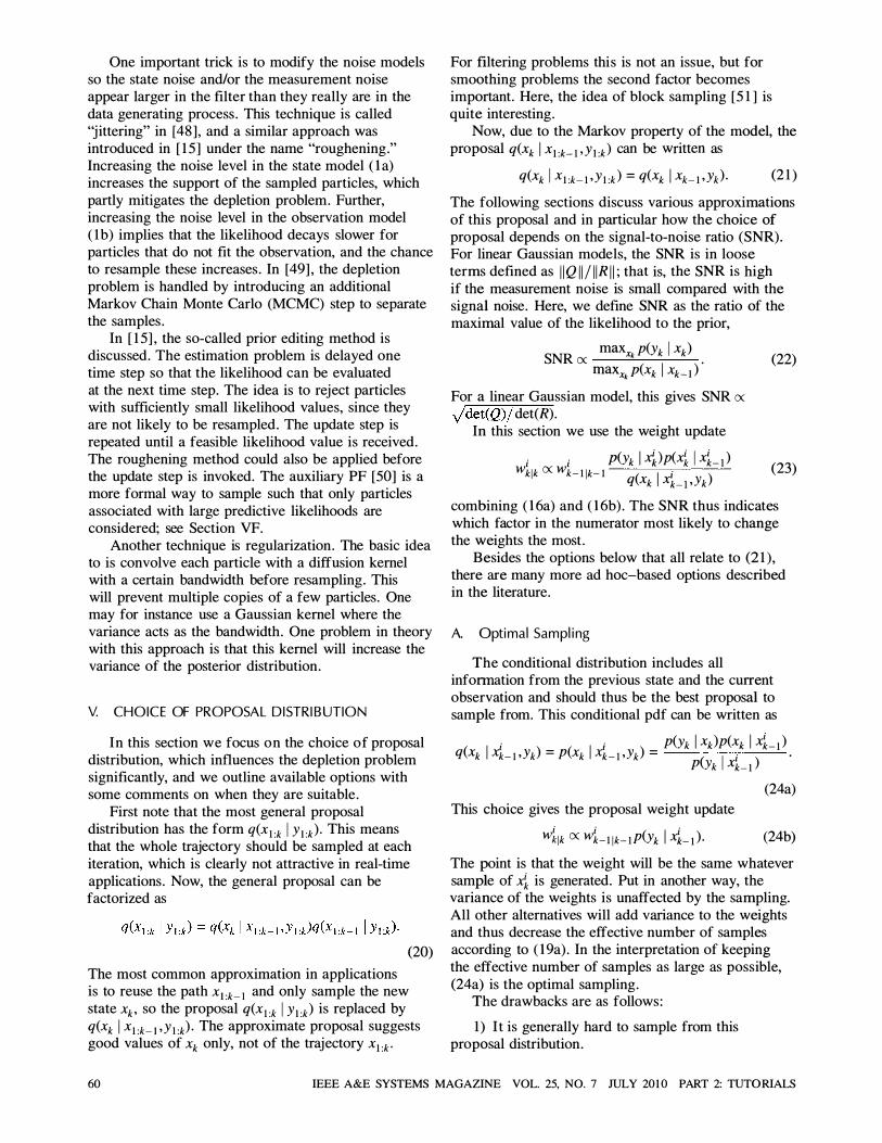
>< 1 1Bt

� 0: O '�L==::::::;::=====:::::::::==::::;:=====-..l -1 -0.5 0 0.5 1.5 2 2.5 3

x

x

x Fig. 2. Illustration of (24a) for scalar state and observation

model. State dynamics moves particle to xk = I and adds uncertainty with variance I, after which observation

Yk = 0.7 = xk + ek is taken. Posterior in this high SNR example is here essentially equal to likelihood.

3

2.5

2

1.5

�

0.5

0

-0.5

-1 -1 -0.5 0.5 1 1.5 2.5 x1

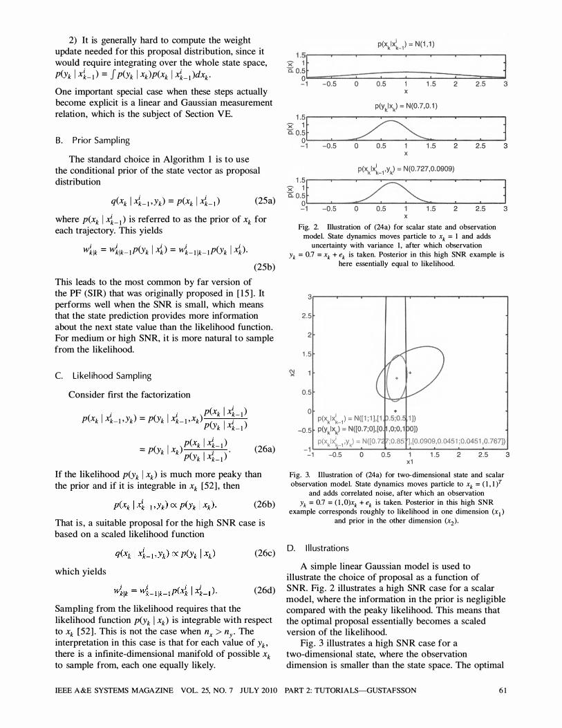
Fig. 3. Illustration of (24a) for two-dimensional state and scalar observation model. State dynamics moves particle to xk = (1, I)T

and adds correlated noise, after which an observation Yk = 0.7 = (1,O)xk + ek is taken. Posterior in this high SNR

example corresponds roughly to likelihood in one dimension (XI) and prior in the other dimension (x2).

D. I llustrations

A simple linear Gaussian model is used to illustrate the choice of proposal as a function of SNR. Fig. 2 illustrates a high SNR case for a scalar model, where the information in the prior is negligible compared with the peaky likelihood. This means that the optimal proposal essentially becomes a scaled version of the likelihood.

Fig. 3 illustrates a high SNR case for a two-dimensional state, where the observation dimension is smaller than the state space. The optimal

IEEE A &E SYSTEMS MAGAZINE VOL. 25, NO. 7 JULY 20 10 PART 2: TUTORIALS-GUSTAFSSON 61

proposal can here be interpreted as the intersection of the prior and likelihood.

E. Optimal Sampli ng with L inearized Li keli hood

The principles illustrated in Figs. 2 and 3 can be used for a linearized model [43] , similar to the measurement update in the EKF (4ef). To simplify the notation somewhat, the process noise in ( 1 a) is assumed additive xk+ l = !(xk) + vk. Assuming that the measurement relation ( 1 b) is linearized as (3b) when evaluating (24a), the optimal proposal can be approximated with

q(xk I XL1'Yk) = N(f(xLl ) + K�(Yk - y�), (HVRkHi + QL1)t ) (27a)

where t denotes pseudoinverse. The Kalman gain, linearized measurement model, and measurement prediction, respectively, are given by

Ki Q ui,T(RiQ Ri,T + R )-1 k = k-1Hk k k-l k k

y� = h(f(xLl ))· The weights should thus be multiplied by the following likelihood in the measurement update:

(27b)

(27c)

(27d)

(27e)

The modifications of (27) can be motivated intuitively as follows. At time k - 1 , each particle corresponds to a state estimate with no uncertainty. The EKF recursions (4) using this initial value gives

Xk-1Ik-1 ",N(4_1'0)::::} (28a)

xklk-1 = !(4-1 ) (28b)

lllk-l = Qk-l (28c)

Kk = Qk_1H[(HkQk_1H[ + Rk)-1 (28d)

xklk = xklk-l + Kk(Yk - h(Xklk-l )) (28e)

llik = Qk-l - KkHkQk-l · (28f)

We denote this sampling strategy OPT-EKF. To compare it with standard SIR algorithm, one can interpret the difference in terms of the time update. The modification in Algorithm 1 assuming a Gaussian distribution for both process and measurement noise, is to make the following substitution in the time update

4+1 = !(x�) + v� SIR : v� '" N(O,Qk)

(29a)

(29b)

OPT-EKF : v� E N(K�+ l (Yk+ l - h(f(x�))) , (Hi�lRtlHi+ l + Qk)t).

and measurement update

SIR : W�lk = WL1Ik-1N(Yk - h(x�) ,Rk)

(29c)

(29d)

OPT-EKF : W�lk = WL11k-1N(Yk - h(f(4-1))' HiQk-1HV + Rk)

(2ge)

respectively. For OPT-SIR, the SNR definition can be more precisely stated as

We make the following observations and interpretations on some limiting cases of these algebraic expressons:

(30)

1 ) For small SNR, K� � 0 in (27b) and

(HVRkHi + QL1 )t � Qk-l in (29c), which shows that the resampling (29c) in OPT-EKF proposal approaches (29b) in SIR as the SNR goes to zero. That is, for low SNR the approximation approaches prior sampling in Section VB.

2) Conversely, for large SNR and assuming Hi invertible (implicitly implying ny � nx) ' then

(HV RkHl + QL1 )t � Hi,-l RkHi,-T in (29c) . Here, all information about the state is taken from the measurement, and the model is not used; that is, for high SNR the approximation approaches likelihood sampling in Section VC.

3) The pseudoinverse t is used consequentlr in the notation for the proposal covariance (HV RkHl +

QL1)t instead of inverse to accomodate the following cases :

a) singular process noise Qk-l ' which is the case in most dynamic models including integrated noise,

b) singular measurement noise Rk, to allow ficticious measurements that model state constraints. For instance, a known state constraint corresponds to infinite information in a subspace of the state space, and the corresponding eigenvector of the measurement information H1RkHV will overwrite the prior information QL1.

F. Auxiliary Sampli ng

The auxiliary sampling proposal resampling filter [50] uses an auxiliary index in the proposal distribution q(xk, i I Yl:k). This leads to an algorithm


that first generates a large number M (typically M = ION) of pairs {x;{,ij}f=,I. From Bayes' rule, we have

p(xk,i I Yl:k)""'" P(Yk I xk)P(xk,i I Yl:k-I) (3 Ia)

= P(Yk I xk)P(xk I i'Yl:k_I)P(i I YI:k-l ) (3 Ib)

= P(Yk I xk)P(xk Ixi-l)wLl 1k-l · (3 I c)

This density is implicit in xk and thus not useful as an proposal density, since it requires xk to be known. The general idea is to find an approximation of

P(Yk I xLI) = J P(Yk I xk)P(xk I xLI)dxk· A simple though useful approximation is to replace xk with its estimate and thus let P(Yk I xL I) = P(Yk I iD above. This leads to the proposal

q(xk,i I Y!:k) = p(Yk I ii)p(xk Ixi-l )wLl1k-l · (3 I d)

Here, Xi = E(xk I xL I) can be the conditional mean or Xi '" P(xk I xLI) a sample from the prior. The new samples are drawn from the marginalized density

X;{""'" P(Xk I Y!:k) = 2:p(xk,i I Y!:k)· (3 Ie)

To evalute the proposal weight, we first take Bayes rule which gives

q(xk,i I Y!:k) = q(i I YI:k)q(xk I i'Yl:k)· (3 1f)

Here, another choice must be made. The latter proposal factor should be defined as

q(xk I i'Yl:k) = P(xk I xLI)· (3 I g)

Then, this factor cancels out when forming

q(i I Yl:k) ex P(Yk I Xi)wLl 1k-l. (3 Ih)

The new weights are thus given by

i iJ P(Yk I x;{)p(x;{ I xLI) Wklk = Wk-Ilk-I (-j .j I ) q Xk,l Yl:k

(3 I i)

Note that this proposal distribution is a product of the prior and the likelihood. The likelihood has the ability to punish samples xi that give a poor match to the most current observation, unlike SIR and SIS where such samples are drawn and then immediately rejected. There is a link between the auxiliary PF and the standard SIR as pointed out in [53] , which is useful for understanding its theoretical properties .

VI. THEORETICA L P ERFORMANCE

The key questions here are how well the PF filtering density P(XI:k I Yl:k) approximates the true posterior p(xl:k I Yl:k)' and what the fundamental mean square error (MSE) bounds for the true posterior are.

A. Convergence I ssues

The convergence properties of the PF are well understood on a theoretical level, see the survey [54] and the book [55 ] . The key question is how well a function g(xk) of the state can be approximated g(Xk) by the PF compared with the conditional expectation E(g(xk»' where

(32)

N g(Xk) = J g(xk)P(xl :k I Yl:k)dxl :k = 2: wi1kg(xi)·

i=1

(33) In short, the following key results exist.

I) Almost sure weak convergence

Nlim p(Xl:k I Yl :k) = p(xl:k I Yl:k) (34) ->00

in the sense that limN->oo g(Xk) = E(g(xk». 2) MSE asymptotic convergence

E(g(Xk) - E(g(Xk»)2 :<:; Pk IIg�k)llsup (35)

where the supremum norm of g(xk) is used. As shown in [55] using the Feynman-Kac formula, under certain regularity and mixing conditions, the constant Pk =

P < 00 does not increase in time. The main condition [54, 55] for this result is that the unnormalized weight function is bounded. Further, most convergence results as surveyed in [56] are restricted to bounded functions of the state g(x) such that Ig(x)1 < C for some C. The convergence result presented in [57] extends this to unbounded functions, for instance estimation of the state itself g(x) = x, where the proof requires the additional assumption that the likelihood function is bounded from below by a constant.

In general, the constant Pk grows polynomially in time, but does not necessarily depend on the dimension of the state space, at least not explicitly. That is, in theory we can expect the same good performance for high-order state vectors. In practice, the performance degrades quickly with the state dimension due to the curse of dimensionality. However, it scales much better with state dimension than the PMF, which is one of the key reasons for the success of the PF.

B. Nonl inear F i lteri ng Performance Bound

Besides the performance bound of a specific algorithm as discussed in the previous section, there are more fundamental estimation bounds for nonlinear filtering that depend only on the model and not on the applied algorithm. The Cramer-Rao Lower Bound (CRLB) lklk provides such a performance bound for


any unbiased estimator Xklk' cov(Xklk) � ��RLB . (36)

The most useful version of CRLB is computed recursively by a Riccati equation which has the same functional form as the KF in (4) evaluated at the true trajectory xt:k'

RCRLB _ RCRLB RCRLBH( o)T klk - klk-l - klk-l Xk X (H(Xv��B HT (xV + Rk)-l H(XV��B

(37a)

��1fuB = F (XV��RLB FT (xV + G(xVQkG(x"l. (37b)

The following remarks summarize the CRLB theory with respect to the PF:

I) For a linear Gaussian model

xk+ l = Fkxk + Gkvk' vk rvN(O,Qk) (38a)

Yk = Hkxk + ek' ek rv N(O,Rk) (38b)

the KF covariance � Ik coincides with lk�RLB. That is, the CRLB bound is attainable in the linear Gaussian case.

2) In the linear non-Gaussian case, the covariances Qk' Rk, and Po are replaced with the inverse intrinsic accuracies I;/, I;,/ and I�l, respectively. Intrinsic accuracy is defined as the Fisher information with respect to the location parameter, and the inverse intrinsic accuracy is always smaller than the covariance. As a consequence of this, the CRLB is always smaller for non-Gaussian noise than for Gaussian noise with the same covariance. See [58] for the details.

3) The parametric CRLB is a function of the true state trajectory x�:k and can thus be computed only in simulations or when ground truth is available from a reference system.

4) The posterior CRLB is the parametric CRLB averaged over all possible trajectories lkf�stCRLB =

E(lkf:reRLB). The expectation makes its computation quite complex in general.

5) In the linear Gaussian case, the parametric and posterior bounds coincide.

6) The covariance of the state estimate from the PF is bounded by the CRLB . The CRLB theory also says that the PF estimate attains the CRLB bound asymptotically in both the number of particles and the information in the model (basically the SNR).

Consult [59] for details on these issues.

V I I . COM PLEXITY BOTILE N ECKS

It is instructive and recommended to generate a profile report from an implementation of the PE Quite

often, unexpected bottlenecks are discovered that can be improved with a little extra work.

A. Resampl ing

One real bottleneck is the resampling step. This crucial step has to be performed at least regularly when Neff becomes too small.

The resampling can be efficiently implemented using a classical algorithm for sampling N ordered independent identically distributed variables according to [60] , commonly referred to as Ripley' s method:

function [x,w]=resample(x,w)

% Multinomial sampling with Ripley's method

u=cumprod(rand(l ,N). A (1.1 [N: -1: 1]»;

u=fliplr(u) ;

wc=cumsum(w) ;

k=l;

for i=l:N

while(wc(k)<u(i»

k=k+1;

end

ind(i)=k;

end

x=x(ind,:);

w=ones (1 , N) • IN;

The complexity of this algorithm is linear in the number of particles N , which cannot be beaten if the implementation is done at a sufficiently low level. For this reason this is the most frequently suggested algorithm also in the PF literature. However, in engineering programming languages such as MATLAB TM, vectorized computations are often an order of magnitude faster than code based on "for" and "while" loops.

The following code also implements the resampling needed in the PF by completely avoiding loops.

function [x,w]=resample(x,w)

% Multinomial sampling with sort

u=rand(N, 1);

wc=cumsum(w) ;

wc=wc/wc(N) ;

[dum,ind1]=sort([u;wc]);

ind2=find(ind1<=N);

ind=ind2-(O:N-1)';

x=x(ind,:) ;

w=ones (1, N) ./N;

This implementation relies on the efficient implementation of sort. Note that sorting is of complexity N log2(N) for low-level implementations, so in theory it should not be an alternative to Ripley' s method for sufficiently large N . However, as Fig. 4 illustrates, the sort algorithm is a factor of five faster for one instance of a vector-oriented programming


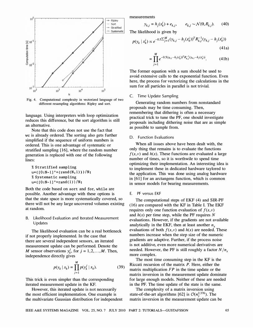
100

��,.--��,.--��...,..,..,., ,-------,

-+- Rlpley Sort

-- Stratified -e- Systematic

10-3 '---��""'"'-��

102 103 104 105 N

Fig. 4. Computational complexity in vectorized language of two different resampling algorithms: Ripley and sort.

language. Using interpreters with loop optimization reduces this difference, but the sort algorithm is still an alternative.

Note that this code does not use the fact that wc is already ordered_ The sorting also gets further simplified if the sequence of uniform numbers is ordered. This is one advantage of systematic or stratified sampling [ 1 6] , where the random number generation is replaced with one of the following lines:

% Stratified sampling

u=([O:N-l ) '+(rand(N,l » )/N;

% Systematic sampling

u=([O:N-l ) '+rand(l » /N;

Both the code based on sort and for, while are possible. Another advantage with these options is that the state space is more systematically covered, so there will not be any large uncovered volumes existing at random.

B. Li keli hood Evaluation and Iterated Measurement Updates

The likelihood evaluation can be a real bottleneck if not properly implemented. In the case that there are several independent sensors, an iterated measurement update can be performed. Denote the M sensor observations yi , for j = 1 , 2, ... , M. Then, independence directly gives

M p(Yk I xk) = II p(yi I xk)·

j= l This trick is even simpler than the corresponding iterated measurement update in the KF.

(39)

However, this iterated update is not necessarily the most efficient implementation. One example is the multivariate Gaussian distribution for independent

measurements

Yk . = h . (xi) + ek . , ,J J ,J

The likelihood is given by

(40)

P(Yk I xi} ex e -O.5�� 1 (Yk,j - h/xDf R;;:) (Yk,j - h/xD) (4 1 a)

M = II e-O.5(yk.j -hj (xDlRk.; (Ykrhj(x�» . (4 1b) j= l

The former equation with a sum should be used to avoid extensive calls to the exponential function. Even here, the process for vectorizing the calculations in the sum for all particles in parallel is not trivial.

C. Time Update Sampli ng

Generating random numbers from nonstandard proposals may be time consuming. Then, remembering that dithering is often a necessary practical trick to tune the PF, one should investigate proposals including dithering noise that are as simple as possible to sample from.

D. Fu nction Evaluations

When all issues above have been dealt with, the only thing that remains is to evaluate the functions f(x, v) and hex). These functions are evaluated a large number of times, so it is worthwile to spend time optimizing their implementation. An interesting idea is to implement these in dedicated hardware taylored to the application. This was done using analog hardware in [6 1 ] for an arctangens function, which is common in sensor models for bearing measurements.

E. PF versus E KF

The computational steps of EKF (4) and SIR-PF ( 1 6) are compared with the KF in Table I. The EKF requires only one function evaluation of f(x, v) and hex) per time step, while the PF requires N evaluations. However, if the gradients are not available analytically in the EKF, then at least another nx evaluations of both f(x, v) and hex) are needed. These numbers increase when the step size of the numeric gradients are adaptive. Further, if the process noise is not additive, even more numerical derivatives are needed. However, the PF is still roughly a factor N /nx more complex.

The most time consuming step in the KF is the Riccati recursion of the matrix P. Here, either the matrix multiplication F P in the time update or the matrix inversion in the measurement update dominate for large enough models . Neither of these are needed in the PF. The time update of the state is the same.

The complexity of a matrix inversion using state-of-the-art algorithms [62] is O(n;.376) . The matrix inversion in the measurement update can be


TABLE I Comparison of EKF in (4) and SIR-PF in (16): Main

Computational Steps

Algorithm Extended Kalman filter

Time update F = 8f(x, v)

G = 8f(x, v)

8x ' 8v

Measurement

update

Estimation

Resampling

x : = f(x, O)

P : = FPFT + GQGT

H = 8h(x)

8x

K = PHT (HPHT + R)- I

x : = x + K(y - h(x))

P : = P - KHP

x = x

Particle filter

N x = L wixi

i= 1

N xi � L wi6(x - xj)

j= 1

avoided using the iterated measurement update. The condition is that the covariance matrix Rk is (block-) diagonal.

As a first-order approximation for large nx ' the KF is O(n�) from the matrix multiplication F P, while the PF is O(N n;) for a typical dynamic model where all elements of f(x, v) depend on all states, for instance the linear model f(x, v) = Fx + v. Also from this perspective, the PF is a factor N /nx computationally more demanding than the EKF.

VI I I . MARG I NALIZED PARTICLE F I LTER THEORY

The main purpose of the marginalized PF (MPF) is to keep the state dimension small enough for the PF to be feasible. The resulting filter is called the MPF or the Rao-Blackwellized PF (RBPF), and it has been known for quite some time under different names, see, e.g. , [49, 63-68].

The MPF utilizes possible linear Gaussian substructures in the model ( 1 ). The state vector is assumed partitioned as xk = « xZl, (xiYl where xi enters both the dynamic model and the observation model linearly. We refer a bit informally to xi as the linear state and xZ as the nonlinear state. MPF essentially represents xZ with particles and applies one KF per particle. The KF provides the conditional distribution for xi conditioned on the trajectory x1:k of nonlinear states and the past observations.

A. Model Structu re

A rather general model, containing a conditionally linear Gaussian substructure is given by

xZ+l = ft(xZ) + Ft(xZ)xi + GJ:(xZ)vJ: Xi+l = fi(xJ:) + Fi(xZ)xi + Gi(xZ)vi Yk = hk(xZ) + Hk(xZ)xi + ek'

The state vector and Gaussian state noise are partitioned as

vk = (:1 ) �N(O,Qk)

( QJ: Qin ) Qk = (Qin)k Qi .

(42a)

(42b)

(42c)

(42d)

Furthermore, x& is assumed Gaussian, xb � N(xo,Po). The density of XO can be arbitrary, but it is assumed known. The underlying purpose with this model structure is that conditioned on the sequence xJ:k' (42) is linear in xi with Gaussian prior, process noise, and measurement noise, respectively, so the KF theory applies.

B . Algorith m Overview

The MPF relies on the following key factorization:

P(XLxJ:k I Y1 :k) = p(xi I xJ:k'Yl:k)p(x1:k I Yl:k) ' (43)

These two factors decompose the nonlinear filtering task into two subproblems:

1) A KF operating on the conditionally linear, Gaussian model (42) provides the exact conditional posterior p(xi I xJ:k'Y1 :k) = N(xi ;iilk(x7�i ),P�k(x7�i»· Here, (42a) becomes an extra measurement for the KF with xk+l -ft(xZ) acting as the observation.

2) A PF estimates the filtering density of the nonlinear states. This involves a nontrivial marginalization step by integrating over the state space of all xi using the law of total probability

P(xJ:k+l I Y1 :k) = P(xJ:k I Y1 :k)P(xJ:+l I xJ:k'Y!:k) = P(xJ:k I Yl:k) J P(XJ:+1 I XLxJ:k'Yl:k)

x p(xi I x1:k'Y!:k)dxi

= p(x1:k I Yl:k) J P(xZ+ l I xi,xJ:k'Yl:k) X N(xi ;xilk(x7�i),P�k(x7�i»dxi. (44)

The intuitive interpretation of this result is that the linear state estimate acts as an extra state noise in (42a) when performing the PF time update.

The time and measurement updates of KF and PF are interleaved, so the timing is important. The information structure in the recursion is described in Algorithm 2. Table II summarizes the information steps in Algorithm 2. Note that the time index appears

66 IEEE A&E SYSTEMS MAG AZINE VOL. 25, NO. 7 JULY 2010 PART 2: TUTORIALS

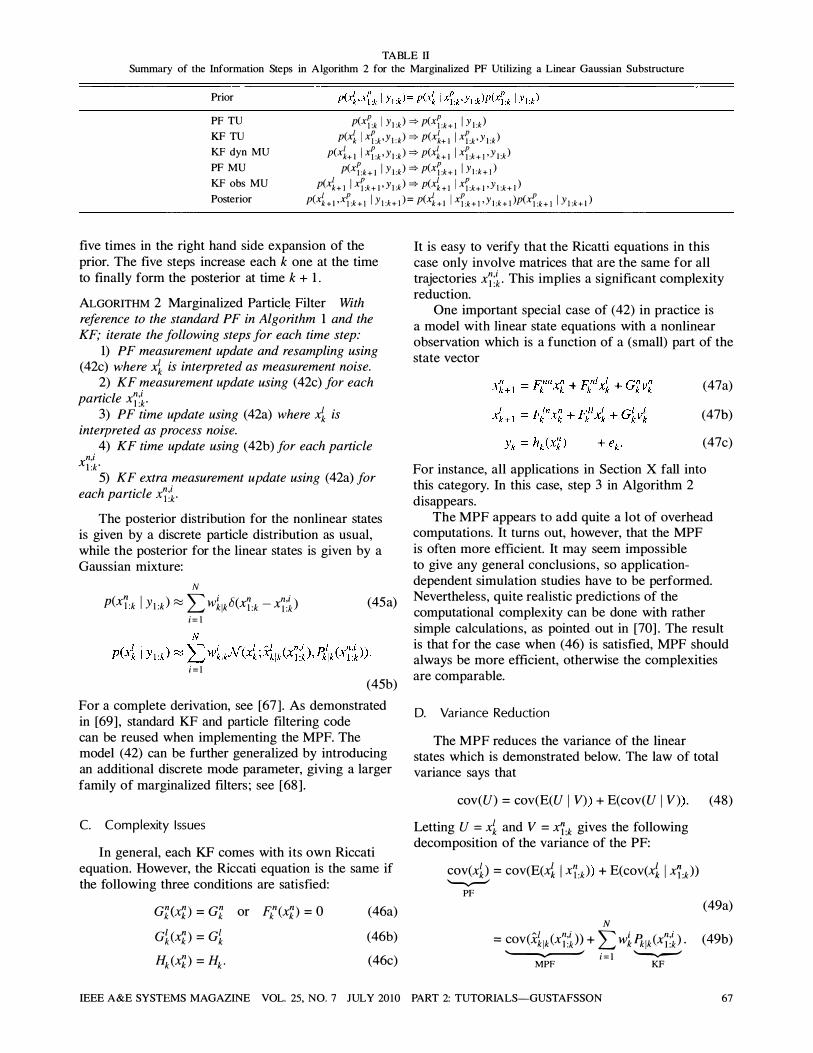
TABLE II Summary of the Information Steps in Algorithm 2 for the Marginalized PF Utilizing a Linear Gaussian Substructure

Prior

PF TU

KF TU P(xf:k I hk) '* P(xf:k+ l I Y l :k )

KF dyn MU

PF MU

KF obs MU

Posterior

p(xi I xf:k ,hk) '* p(xi+ 1 I xf,k ' Y l :k ) P(xi+ l l xf:k ,hk ) '* PCxi+ l l xf:k + l ' Y l :k )

P(xf:k + l I Y l :k ) '* P(xf:k+ l I hk+ l ) P(xi+ l I xf:k+ l ' hk ) '* P(xi + l I xf,k+ l 'hk+ l )

P(xi + l ,xf,k + 1 I Yl :k+ I ) = P(xi + l I xf:k+ l ' Y l :k + I )P(xf,k + l I YI :k+ l )

five times in the right hand side expansion of the prior. The five steps increase each k one at the time to finally form the posterior at time k + 1 .

ALGORITHM 2 Marginalized Particle Filter With reference to the standard PF in Algorithm 1 and the KF; iterate the following steps for each time step:

1) PF measurement update and resampling using (42c) where xi is interpreted as measurement noise.

2) KF measurement update using (42c) for each . I n i partlc e xl �k .

3) PF time update using (42a) where xi is interpreted as process noise.

4) KF time update using (42b) for each particle n,i x1 :k •

5) KF extra measurement update using (42a) for h . I n i eac partlc e X l �k .

The posterior distribution for the nonlinear states is given by a discrete particle distribution as usual, while the posterior for the linear states is given by a Gaussian mixture:

N

p(x1:k I Y\ :k ) � L wklk8(xl:k - x:�� ) (45a) i = 1

i = 1 (45b)

For a complete derivation, see [67] . As demonstrated in [69] , standard KF and particle filtering code can be reused when implementing the MPF. The model (42) can be further generalized by introducing an additional discrete mode parameter, giving a larger family of marginalized filters ; see [68] .

C. Complexity Issues

In general, each KF comes with its own Riccati equation. However, the Riccati equation is the same if the following three conditions are satisfied:

GI:(xf:) = GI: or Ft(xl:) = 0

Gi(xk ) = Gi

Hk (xf: ) = Hk •

(46a)

(46b)

(46c)

It is easy to verify that the Ricatti equations in this case only involve matrices that are the same for all trajectories x7�� . This implies a significant complexity reduction.

One important special case of (42) in practice is a model with linear state equations with a nonlinear observation which is a function of a (small) part of the state vector

(47a)

(47b)

(47c)

For instance, all applications in Section X fall into this category. In this case, step 3 in Algorithm 2 disappears.

The MPF appears to add quite a lot of overhead computations. It turns out, however, that the MPF is often more efficient. It may seem impossible to give any general conclusions, so applicationdependent simulation studies have to be performed. Nevertheless, quite realistic predictions of the computational complexity can be done with rather simple calculations, as pointed out in [70] . The result is that for the case when (46) is satisfied, MPF should always be more efficient, otherwise the complexities are comparable.

D. Variance Red uction

The MPF reduces the variance of the linear states which is demonstrated below. The law of total variance says that

cov(U) = cov(E(U I V» + E(cov(U I V» . (48)

Letting U = xi and V = X\:k gives the following decomposition of the variance of the PF:

cov(xi> = cov(E(xi I xl:k» + E(cov(xi I x!:k» "-v-"

PF

N (49a)

= COV(Xi lk (x7��» + L WU1Ik (x7�� ) . (49b) � i = 1 '-v--"

MPF KF

IEEE A&E SYSTEMS MAGAZINE VOL. 25, NO. 7 JULY 2010 PART 2: TUTORIALS-GUSTAFSSON 67

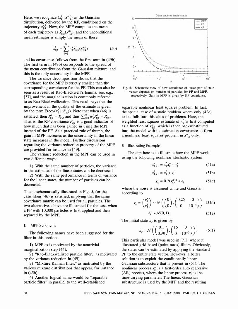
Here, we recognize (xi I x�;�) as the Gaussian distribution, delivered by the KF, conditioned on the trajectory �;� . Now, the MPF computes the mean of each trajectory as xi lk (x�;� ) , and the unconditional mean estimator is simply the mean of these,

N Xi1k = L w�xilk (X�;�) (50)

; = 1

and its covariance follows from the first term in (49b). The first term in (49b) corresponds to the spread of the mean contribution from the Gaussian mixture, and this is the only uncertainty in the MPF.

The variance decomposition shows that the covariance for the MPF is strictly smaller than the corresponding covariance for the PF. This can also be seen as a result of Rao-Blackwell' s lemma, see, e.g. , [37] , and the marginalization is commonly referred to as Rao-Blackwellization. This result says that the improvement in the quality of the estimate is given by the term E(cov(xi I x1:k)) . Note that when (46) is satisfied, then P�lk = llik and thus 2:;:'1 WkP�lk = llik ' That is, the KF covariance llik is a good indicator of how much that has been gained in using the MPF instead of the PF. As a practical rule of thumb, the gain in MPF increases as the uncertainty in the linear state increases in the model. Further discussions regarding the variance reduction property of the MPF are provided for instance in [49] .

The variance reduction in the MPF can be used in two different ways:

1) With the same number of particles, the variance in the estimates of the linear states can be decreased.

2) With the same performance in terms of variance for the linear states, the number of particles can be decreased. This is schematically illustrated in Fig. 5, for the case when (46) is satisfied, implying that the same covariance matrix can be used for all particles . The two alternatives above are illustrated for the case when a PF with 10,000 particles is first applied and then replaced by the MPF.

E. MPF Synonyms

The following names have been suggested for the filter in this section:

1) MPF as is motivated by the nontrivial marginalization step (44).

2) "Rao-Blackwellized particle filter," as motivated by the variance reduction in (49) .

3) "Mixture Kalman filter," as motivated by the various mixture distributions that appear, for instance in (45b).

4) Another logical name would be "separable particle filter" in parallel to the well-established

Covariance for linear slales 1 2r---------�--------�----r===�

- MPF PF

1 0 -+- KF

o�--------��--------�--------� 1 � 1 � 1 � 1 �

N

Fig. 5 . Schematic view of how covariance of linear part of state vector depends on number of particles for PF and MPF,

respectively. Gain in MPF is given by KF covariance.

separable nonlinear least squares problem. In fact, the special case of a static problem where only (42c) exists falls into this class of problems. Here, the weighted least squares estimate of xi is first computed as a function of x1:k ' which is then backsubstituted into the model with its estimation covariance to form a nonlinear least squares problem in x):k only.

F. I llustrati ng Example

The aim here is to illustrate how the MPF works using the following nonlinear stochastic system

n _ I n n xk+ l - xkxk + Vk I I I xk+ 1 = xk + Vk Yk = 0.2(xk)2 + ek

where the noise is assumed white and Gaussian according to

(5 I a)

(S I b)

(S I c)

v = (VI: ) "VN ( (O) (0.25 0 ) ) (S I d) k vk 0 ' ° 10-4

ek "V N(O, 1 ) . (5 1 e)

The initial state Xo is given by

xo "VN ( (�� ) , ( �6 I�-3 ) ) ' (5 1 f)

This particular model was used i n [7 1 ] , where it illustrated grid-based (point-mass) filters. Obviously, the states can be estimated by applying the standard PF to the entire state vector. However, a better solution is to exploit the conditionally linear, Gaussian substructure that is present in (5 1 ) . The nonlinear process xl: is a first-order auto regressive (AR) process, where the linear process xi is the time-varying parameter. The linear, Gaussian substructure is used by the MPF and the resulting

68 IEEE A&E SYSTEMS MAGAZINE VOL. 25, NO. 7 JULY 20 1 0 PART 2: TUTORIALS

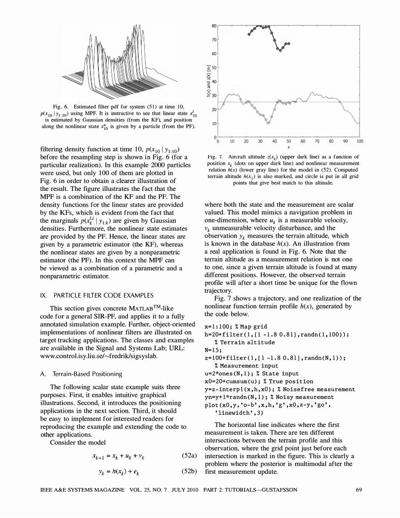
Fig. 6. Estimated filter pdf for system (5 1 ) at time 1 0,

P(XIO I Yl : lo) using MPF. It is instructive to see that linear state X;o is estimated by Gaussian densities (from the KF), and position

along the nonlinear state xto is given by a particle (from the PF) .

filtering density function at time 1 0, P(xlO I Yl : lo) before the resampling step is shown in Fig. 6 (for a particular realization) . In this example 2000 particles were used, but only 1 00 of them are plotted in Fig. 6 in order to obtain a clearer illustration of the result. The figure illustrates the fact that the MPF is a combination of the KF and the PF. The density functions for the linear states are provided by the KFs, which is evident from the fact that the marginals p(xti I Yl :k) are given by Gaussian densities . Furthermore, the nonlinear state estimates are provided by the PF. Hence, the linear states are given by a parametric estimator (the KF), whereas the nonlinear states are given by a nonparametric estimator (the PF) . In this context the MPF can be viewed as a combination of a parametric and a nonparametric estimator.

IX. PA RTICLE F I LTER CO D E EXAM PLES

This section gives concrete MATLABTM-like code for a general SIR-PF, and applies it to a fully annotated simulation example. Further, object-oriented implementations of nonlinear filters are illustrated on target tracking applications . The classes and examples are available in the Signal and Systems Lab; URL: www.control.isy.liu.se/..-Ifredriklsigsyslab.

A. Terrai n-Based Position i ng

The following scalar state example suits three purposes. First, it enables intuitive graphical illustrations. Second, it introduces the positioning applications in the next section. Third, it should be easy to implement for interested readers for reproducing the example and extending the code to other applications.

Consider the model

(S2a)

(S2b)

� so

o�----------�--�------�----------�--� o w w � � � ro ro 00 W � x

Pig. 7. Aircraft altitude z(xk) (upper dark line) as a function of position xk (dots on upper dark line) and nonlinear measurement relation hex) (lower gray line) for the model in (52). Computed terrain altitude h(x ) ) is also marked, and circle is put in all grid

points that give best match to this altitude.

where both the state and the measurement are scalar valued. This model mimics a navigation problem in one-dimension, where Uk is a measurable velocity, vk unmeasurable velocity disturbance, and the observation Yk measures the terrain altitude, which is known in the database h(x) . An illustration from a real application is found in Fig. 6. Note that the terrain altitude as a measurement relation is not one to one, since a given terrain altitude is found at many different positions. However, the observed terrain profile will after a short time be unique for the flown trajectory.

Fig. 7 shows a trajectory, and one realization of the nonlinear function terrain profile h(x), generated by the code below.

x=l: 100; % Map grid

h=20+filter(l, [1 -1.8 0.8 1 1 ,randn(l,100» ;

% Terrain altitude

N=15;

z=100+filter(l, [1 -1. 8 0.81 1 , randn(N, 1» ;

% Measurement input

u=2*ones (N, 1); % State input

xO=20+cumsum(u); % True position

y=z-interpl (x,h,xO); % Noisefree measurement

yn=y+l*randn(N, 1); % Noisy measurement

plot(xO,y,'o-b',x,h,'g',xO,z-y,'go',

'linewidth',3)

The horizontal line indicates where the first measurement is taken. There are ten different intersections between the terrain profile and this observation, where the grid point just before each intersection is marked in the figure. This is clearly a problem where the posterior is multimodal after the first measurement update.

IEEE A&E SYSTEMS MAGAZINE VOL. 25, NO. 7 JULY 20 1 0 PART 2: TUTORIALS-GUSTAFSSON 69

21 ..

�" I • JL • � 0.4 m 0 � 10 20 30

i" l ,

n ,

m 0.4 �

0 10 20 30

t" 1 Ul � 0.4 i= 0 10 20 30

Time k = 1

l�lITll! 40 50 60

Ilfl1® 40 50 60

70

• 70

�NWI! • 80 90

lim 80 90

D' II[I�II 40 50 60 70 80 90

Position x

21 Time k = 15 ..

1 : ; 1 I • • • '---� . • • 100 � 10 20 30 40 50 60 70 80 90 100

I '" c '5. 0.8 E m 0.4 �

0 100 10 20 30 40 50 60 70 80 90 100

I fi! "8. 0.8 " � 0.4 i= 0

100 10 20 30 40 50 60 70 80 90 100 Position x

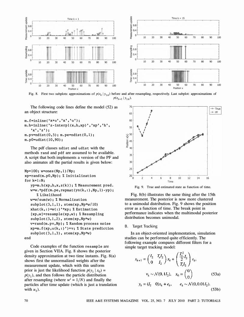
Fig. 8 . First two subplots: approximations of p(xk I Y l :k) before and after resampling, respectively. Last subplot: approximations of

p(xk+ ! I Yl :k) '

The following code lines define the model (52) as an object structure:

m.f=inline( 'x+u', 'x', 'u');

m.h=inline('z-interp1(x,h,xp)','xp' ,'h',

'x','z');

m.pv=ndist(0,5); m.pe=ndist(O,l);

m.pO=udist(10,9 0);

The pdf classes ndist and udist with the methods rand and pdf are assumed to be available. A script that both implements a version of the PF and also animates all the partial results is given below:

Np= 100; w=ones (Np, 1) /Np;

xp=rand(m.pO,Np); % Initialization

for k=l:N;

yp=m.h(xp,h,x, z(k» ; % Measurement pred.

w=w.*pdf(m.pe,repmat(yn(k,:),Np,l)-yp);

% Likelihood

w=w/sum(w); % Normalization

subplot(3,1,1), stem(xp,Np*w/10)

xhat(k,: )=w(:) '*xp; % Estimation

[xp,w]=resample(xp,w); % Resampling

subplot(3,1,2), stem(xp,Np*w)

v=rand(m.pv,Np); % Random process noise

xp=m.f(xp,u(k,:)')+v; % State prediction

subplot(3,1,3), stem(xp,Np*w)

end

Code examples of the function resample are given in Section VIlA. Fig. 8 shows the posterior density approximation at two time instants . Fig. 8(a) shows first the unnormalized weights after the measurement update, which with this uniform prior is just the likelihood function P(Yl I xo) =

P(Yl ) ' and then follows the particle distribution after res amp ling (where wi = 1 / N) and finally the particles after time update (which is just a translation with u1).

70

65 , I

I 60 I

4t I 55 I

\ I 2 50

\ I ';( " c 45 � 40

35

30

25

2 4 6 8 10 Time 12 14

I-- True l -+- PF

16

Fig. 9. True and estimated state as function of time.

Fig. 8(b) illustrates the same thing after the 1 5th measurement. The posterior is now more clustered to a unimodal distribution. Fig. 9 shows the position error as a function of time. The break point in performance indicates when the multimodal posterior distribution becomes unimodal.

B . Target Tracki ng

In an object-oriented implementation, simulation studies can be performed quite efficiently. The following example compares different filters for a simple target tracking model:

(53a)

ek ,...., N(0, 0.01l2) · (53b)

70 IEEE A&E SYSTEMS MAGAZINE VOL. 25, NO. 7 JULY 2010 PART 2: TUTORIALS

The observation model is first linear to be comparable to the KF that provides the optimal estimate. The example makes use of two different objects :

1 ) S ignal object where the state x l :k and observation Yl :k sequences are stored with their associated uncertainty (covariances Ikx, PI or particle representation) . Plot methods in this class can then automatically provide confidence bounds.

2) Model objects for linear and nonlinear models, with methods implementing simulation and filtering algorithms.

The purpose of the following example is to illustrate how little coding is required with this object-oriented approach. First, the model is loaded from an extensive example database as a linear state-space model. It is then converted to the general nonlinear model structure, which does not make use of the fact that the underlying model is linear.

mss=exlti ( 'cv2d') ;

mnl=nl ( mss) ;

Now, the following state trajectories are compared:

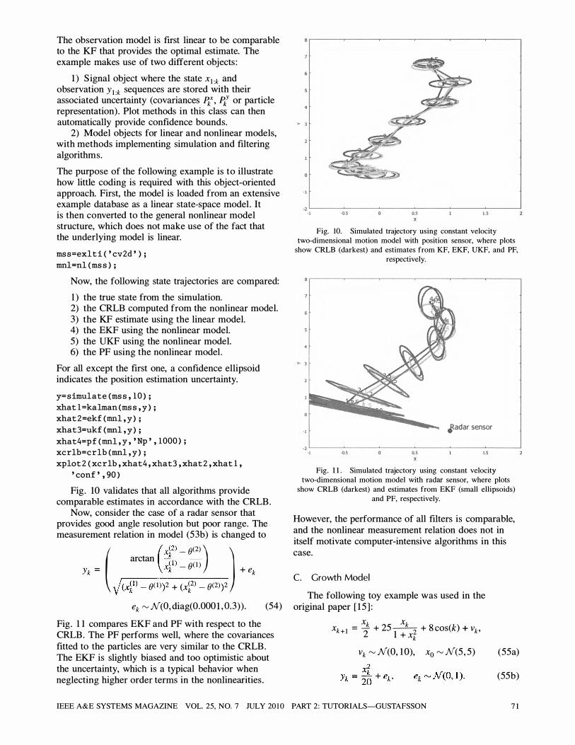
1 ) the true state from the simulation. 2) the CRLB computed from the nonlinear model. 3) the KF estimate using the linear model. 4) the EKF using the nonlinear model. S) the UKF using the nonlinear model. 6) the PF using the nonlinear model.

For all except the first one, a confidence ellipsoid indicates the position estimation uncertainty.

y=simulate ( mss,lO) ;

xhatl=kalman ( mss,y) ;

xhat2=ekf (mnl,y) ;

xhat3=ukf ( mnl,y) ;

xhat4=pf ( mnl,y,'Np',lOOO) ;

xcrlb=crlb ( mnl,y) ;

xplot2 ( xcrlb,xhat4,xhat3,xhat2,xhatl,

'conf',90)

Fig. 10 validates that all algorithms provide comparable estimates in accordance with the CRLB.

Now, consider the case of a radar sensor that provides good angle resolution but poor range. The measurement relation in model (S3b) is changed to

Yk = xk - e(l ) + e ( arctan

(X��: - e(2) ) ) J(x�l ) _ e(1» 2 + (x�2) _ e(2» 2

k

ek ", N(O, diag(O.OOO I , O.3)) . (S4)

Fig. 1 1 compares EKF and PF with respect to the CRLB. The PF performs well, where the covariances fitted to the particles are very similar to the CRLB . The EKF is slightly biased and too optimistic about the uncertainty, which is a typical behavior when neglecting higher order terms in the nonlinearities .

>- 3

- 1

� L-____ � ____ � ____________ � ____ �� ____ � -1 -0.5 0.5 1 .5

Fig. 10_ Simulated trajectory using constant velocity

two-dimensional motion model with position sensor, where plots

show CRLB (darkest) and estimates from KF, EKF, UKF, and PF,

respectively.

-1 jadar sensor _2L-----�----�------------�----��----�

-I -0.5 0.5 1.5

Fig. 1 1 . Simulated trajectory using constant velocity

two-dimensional motion model with radar sensor, where plots

show CRLB (darkest) and estimates from EKF (small ellipsoids)

and PF, respectively_

However, the performance of all filters is comparable, and the nonlinear measurement relation does not in itself motivate computer-intensive algorithms in this case.

C. Growth Model

The following toy example was used in the original paper [ 1 S ] :

Xk xk xk+ l = -2 + 2S--2 + 8 cos(k) + vk ' 1 + xk

vk ", N(O, 10), xo ", N(S , S) (SSa)

(SSb)

IEEE A&E SYSTEMS MAGAZINE VOL. 25, NO. 7 JULY 20 1 0 PART 2: TUTORIALS-GUSTAFSSON 7 1

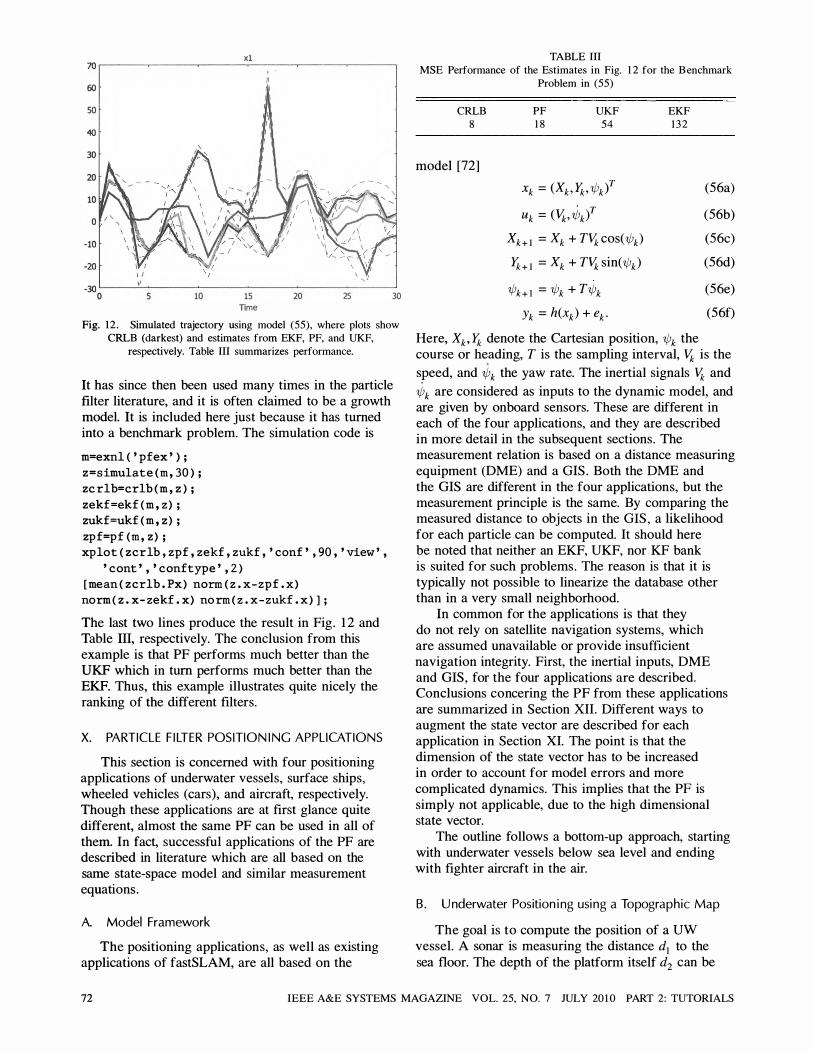
xl �r-----�----�------�----�----�------'

60

50

40

5 10 15 Time

I I I

20 25 30

Fig. 12 . Simulated trajectory using model (55), where plots show

CRLB (darkest) and estimates from EKF, PF, and UKF,

respectively. Table III summarizes performance.

It has since then been used many times in the particle filter literature, and it is often claimed to be a growth model. It is included here just because it has turned into a benchmark problem. The simulation code is

m=exnl( 'pfex');

z=simulate(m,30);

zcrlb=crlb(m,z);

zekf=ekf (m, z) ;

zukf=ukf (m, z) ;

zpf=pf (m, z) ;

xplot(zcrlb,zpf,zekf,zukf,'conf',90, 'view' ,

'cont','conftype',2)

[mean(zcrlb.Px) norm(z.x-zpf.x)

norm(z.x-zekf.x) norm(z.x-zukf.x)] ;

The last two lines produce the result in Fig. 1 2 and Table III, respectively. The conclusion from this example is that PF performs much better than the UKF which in turn performs much better than the EKF. Thus, this example illustrates quite nicely the ranking of the different filters.

X. PARTICLE F I LT E R POS ITI O N I NG APPL ICATIONS

This section is concerned with four positioning applications of underwater vessels, surface ships, wheeled vehicles (cars), and aircraft, respectively. Though these applications are at first glance quite different, almost the same PF can be used in all of them. In fact, successful applications of the PF are described in literature which are all based on the same state-space model and similar measurement equations.

A. Model Framework

The positioning applications, as well as existing applications of fastS LAM, are all based on the

TABLE III

MSE Performance of the Estimates in Fig. 1 2 for the B enchmark

Problem in (55)

CRLB

8

model [72]

PF

1 8

UKF

54

Xk = (Xk , lk, 'l/Jk)T

Uk = (\'k, �kl Xk+ ! = Xk + T\'k cos('l/Jk)

lk+ ! = Xk + T\'k sin( 'l/Jk)

'l/Jk+ 1 = 'l/Jk + T'l/Jk

Yk = h(xk) + ek •

EKF

1 3 2

(56a)

(56b)

(56c)

(56d)

(56e)

(56f)

Here, Xk , lk denote the Cartesian position, 'l/Jk the course or he

.ading, T is the sampling interval, \'k is the

speed, and 'l/Jk the yaw rate. The inertial signals \'k and

'l/Jk are considered as inputs to the dynamic model, and are given by onboard sensors. These are different in each of the four applications, and they are described in more detail in the subsequent sections. The measurement relation is based on a distance measuring equipment (DME) and a GIS . Both the DME and the GIS are different in the four applications, but the measurement principle is the same. By comparing the measured distance to objects in the GIS , a likelihood for each particle can be computed. It should here be noted that neither an EKF, UKF, nor KF bank is suited for such problems. The reason is that it is typically not possible to linearize the database other than in a very small neighborhood.

In common for the applications is that they do not rely on satellite navigation systems, which are assumed unavailable or provide insufficient navigation integrity. First, the inertial inputs, DME and GIS, for the four applications are described. Conclusions con cering the PF from these applications are summarized in Section XII. Different ways to augment the state vector are described for each application in Section XI. The point is that the dimension of the state vector has to be increased in order to account for model errors and more complicated dynamics. This implies that the PF is simply not applicable, due to the high dimensional state vector.

The outline follows a bottom-up approach, starting with underwater vessels below sea level and ending with fighter aircraft in the air.

B . Underwater Position i ng usi ng a Topograph ic Map

The goal is to compute the position of a UW vessel. A sonar is measuring the distance d! to the sea floor. The depth of the platform itself d2 can be


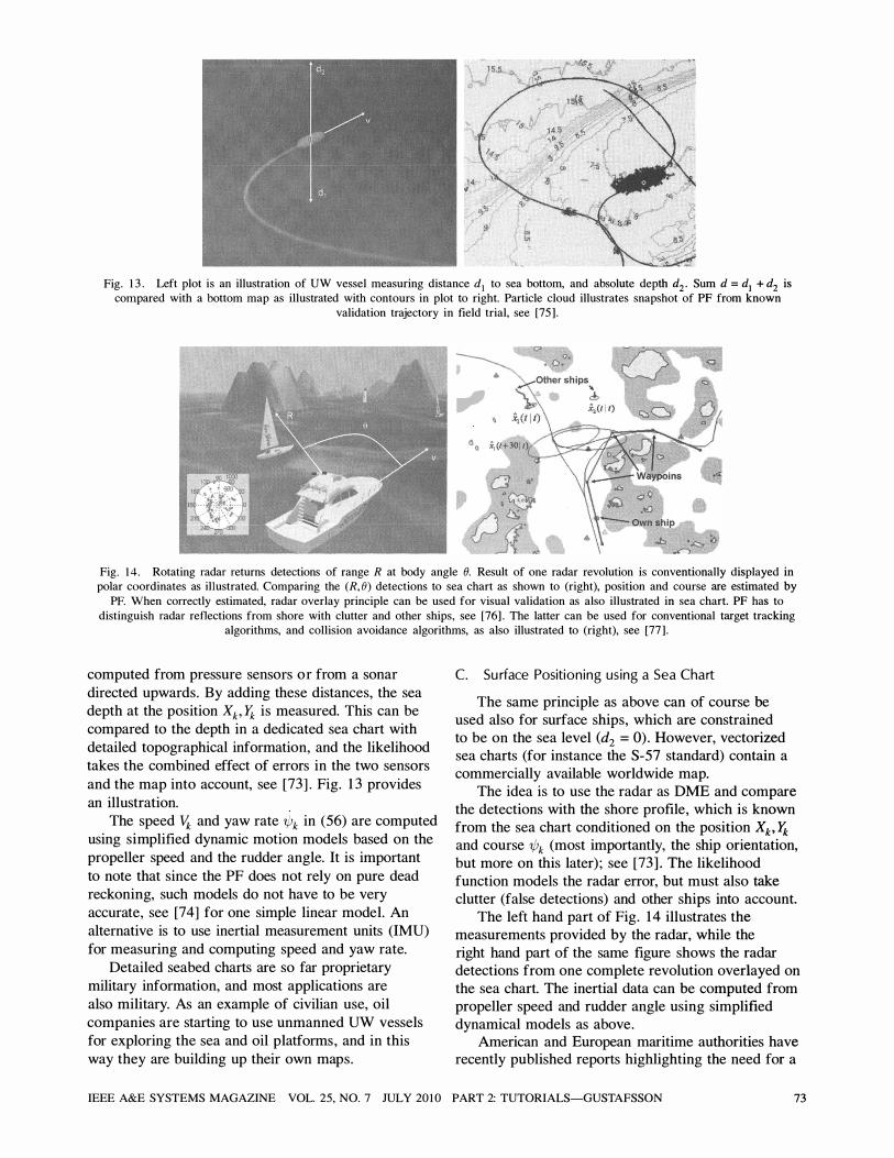
Fig. 1 3 . Left plot is an illustration of UW vessel measuring distance dl to sea bottom, and absolute depth d2 . Sum d = dl + d2 is

compared with a bottom map as illustrated with contours in plot to right. Particle cloud illustrates snapshot of PF from known

validation trajectory in field trial, see [75 ] .

o •

• • D • •

wi' 0 -', (1+ 301 1)( •

Fig . 14. Rotating radar returns detections of range R at body angle B. Result of one radar revolution is conventionally displayed in

polar coordinates as illustrated. Comparing the (R, e) detections to sea chart as shown to (right), position and course are estimated by

PF. When correctly estimated, radar overlay principle can be used for visual validation as also illustrated in sea chart. PF has to

distinguish radar reflections from shore with clutter and other ships, see [76] . The latter can be used for conventional target tracking

algorithms, and collision avoidance algorithms, as also illustrated to (right), see [77 ] .

computed from pressure sensors or from a sonar directed upwards. By adding these distances, the sea depth at the position Xk, lk is measured. This can be compared to the depth in a dedicated sea chart with detailed topographical information, and the likelihood takes the combined effect of errors in the two sensors and the map into account, see [73] . Fig. 1 3 provides an illustration.

The speed Vk and yaw rate 'lj;k in (56) are computed using simplified dynamic motion models based on the propeller speed and the rudder angle. It is important to note that since the PF does not rely on pure dead reckoning, such models do not have to be very accurate, see [74] for one simple linear model. An alternative is to use inertial measurement units (IMU) for measuring and computing speed and yaw rate.

Detailed seabed charts are so far proprietary military information, and most applications are also military. As an example of civilian use, oil companies are starting to use unmanned UW vessels for exploring the sea and oil platforms, and in this way they are building up their own maps.

C. Su rface Position ing us ing a Sea Chart

The same principle as above can of course be used also for surface ships, which are constrained to be on the sea level (d2 = 0) . However, vectorized sea charts (for instance the S-57 standard) contain a commercially available worldwide map.

The idea is to use the radar as DME and compare the detections with the shore profile, which is known from the sea chart conditioned on the position Xk, lk and course 'lj;k (most importantly, the ship orientation, but more on this later) ; see [73] . The likelihood function models the radar error, but must also take clutter (false detections) and other ships into account.

The left hand part of Fig. 14 illustrates the measurements provided by the radar, while the right hand part of the same figure shows the radar detections from one complete revolution overlayed on the sea chart. The inertial data can be computed from propeller speed and rudder angle using simplified dynamical models as above.

American and European maritime authorities have recently published reports highlighting the need for a

IEEE A&E SYSTEMS MAGAZINE VOL. 25, NO. 7 JULY 201 0 PART 2: TUTORlALS-GUSTAFSSON 73

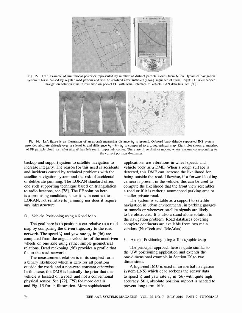
Fig. 1 5 . Left: Example of multimodal posterior represented by number of distinct particle clouds from NIRA Dynamics navigation

system. This is caused by regular road pattern and will be resolved after sufficiently long sequence of turns . Right: PF in embedded

navigation solution runs in real time on pocket PC with serial interface to vehicle CAN data bus, see [80] .

Fig. 1 6. Left figure is an illustration of an aircraft measuring distance hI to ground. Onboard baro-altitude supported INS system

provides absolute altitude over sea level h, and difference h2 = h - hI is compared to a topographical map. Right plot shows a snapshot

of PF particle cloud just after aircraft has left sea in upper left comer. There are three distinct modes, where the one corresponding to

the correct position dominates.

backup and support system to satellite navigation to increase integrity. The reason for this need is accidents and incidents caused by technical problems with the satellite navigation system and the risk of accidental or deliberate jamming. The LORAN standard offers one such supporting technique based on triangulation to radio beacons, see [78] . The PF solution here is a promising candidate, since it is, in contrast to LORAN, not sensitive to jamming nor does it require any infrastructure.

D. Veh icle Position i ng us ing a Road Map

The goal here is to position a car relative to a road map by comparing the driven trajecto�y to the road network. The speed � and yaw rate '¢k in (56) are computed from the angular velocities of the nondriven wheels on one axle using rather simple geometrical relations. Dead reckoning (56) provides a profile that fits to the road network.

The measurement relation is in its simplest form a binary likelihood which is zero for all positions outside the roads and a non-zero constant otherwise. In this case, the DME is basically the prior that the vehicle is located on a road, and not a conventional physical sensor. See [72] , [79] for more details and Fig. 1 5 for an illustration. More sophisticated

applications use vibrations in wheel speeds and vehicle body as a DME. When a rough surface is detected, this DME can increase the likelihood for being outside the road. Likewise, if a forward-looking camera is present in the vehicle, this can be used to compute the likelihood that the front view resembles a road or if it is rather a nonmapped parking area or smaller private road.

The system is suitable as a support to satellite navigation in urban environments, in parking garages or tunnels or whenever satellite signals are likely to be obstructed. It is also a stand-alone solution to the navigation problem. Road databases covering complete continents are available from two main vendors (NavTech and TeleAtlas) .

E . Aircraft Pos ition i ng us ing a Topographic M a p

The principal approach here i s quite similar to the UW positioning application and extends the one-dimensional example in Section IX to two dimensions.

A high-end IMU is used in an inertial navigation system (INS) which dead �eckons the sensor data to speed � and yaw rate '¢k in (56) with quite high accuracy. Still, absolute position support is needed to prevent long-term drifts .


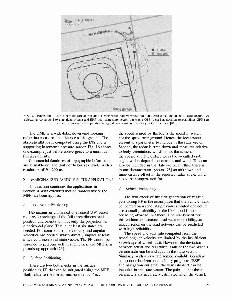
VEl. . 1 1 8 [ ka/b ) B!W(E 1 R�ElR . 0

Parking garage

Fig. 17 . Navigation of car in parking garage. Results for MPF when relative wheel radii and gyro offset are added to state vector. Two trajectories correspond to map-aided system and EKF with same state vector, but where GPS is used as position sensor. Since GPS gets

several drop-outs before parking garage, dead-reckoning trajectory is incorrect; see [8 1 ] .

The DME i s a wide-lobe, downward looking radar that measures the distance to the ground. The absolute altitude is computed using the INS and a supporting barometric pressure sensor. Fig. 1 6 shows one example just before convergence to a unimodal filtering density.

Commercial databases of topographic information are available on land (but not below sea level), with a resolution of 50-200 m.

X I . MARG I NALIZED PARTICLE F I LTER APPL ICATIONS

This section continues the applications in Section X with extended motion models where the MPF has been applied.

A. U nderwater Position i ng

Navigating an unmanned or manned UW vessel requires knowledge of the full three-dimensional position and orientation, not only the projection in a horizontal plane. That is, at least six states are needed. For control, also the velocity and angular velocities are needed, which directly implies at least a twelve-dimensional state vector. The PF cannot be assumed to perform well in such cases, and MPF is a promising approach [73 ] .

B . Su rface Position i ng

There are two bottlenecks in the surface positioning PF that can be mitigated using the MPF. Both relate to the inertial measurements. First,

the speed sensed by the log is the speed in water, not the speed over ground. Hence, the local water current is a parameter to include in the state vector. Second, the radar is strap down and measures relative to body orientation, which is not the same as the course 'ifJk • The difference is the so called crab angle, which depends on currents and wind. This can also be included in the state vector. Further, there is in our demonstrator system [76] an unknown and time-varying offset in the reported radar angle, which has to be compensated for.

C. Veh icle Position i ng

The bottleneck of the first generation of vehicle positioning PF is the assumption that the vehicle must be located on a road. As previously hinted one could use a small probability in the likelihood function for being off-road, but there is no real benefit for this without an accurate dead-reckoning ability, so reoccurrence on the road network can be predicted with high reliability.

The speed and yaw rate computed from the wheel angular velocity are limited by the insufficient knowledge of wheel radii. However, the deviation between actual and real wheel radii of the two wheels on one axle can be included in the state vector. Similarly, with a yaw rate sensor available (standard component in electronic stability programs (ESP) and navigation systems), the yaw rate drift can be included in the state vector. The point is that these parameters are accurately estimated when the vehicle


is on the road, and in the off-road mode, improved dead reckoning can be achieved. Tests in demonstrator vehicles have shown that the exit point from parking garages and parking areas are well estimated, and that shorter unmapped roads are not a problem; see Fig. 17 .

D. Ai rcraft Position ing

The primary role of the terrain based navigation (TERNAV) module is to support the INS with absolute position information. The INS consists of an EKF based on a state vector with over 20 motion states and sensor bias parameters. The current bottleneck is the interface between TERNAV and INS . The reason is that TERNAV outputs a possibly multimodal position density, while the INS EKF expects a Gaussian observation. The natural idea is to integrate both TERNAV and INS into one filter. This gives a high-dimensional state vector, where one measurement (radar altitude) is very nonlinear. The MPF handles this elegantly, by essentially keeping the EKF from the existing INS and using the PF only for the radar altitude measurement.

The altitude radar gives a measurement outlier when the radar pulse is reflected in trees . Tests have validated that a Gaussian mixture where one mode has a positive mean models the real measurement error quite well. This Gaussian mixture distribution can be used in the likelihood computation, but such a distribution is in this case logically modeled by a binary Markov parameter, which is one in positions over forest and zero otherwise. In this way, the positive correlation between outliers is modeled, and a prior from ground-type information in the GIS can be incorporated. This example motivates the inclusion of discrete states in the model framework. See [67] , [68] for the details.

XI I . SU MMARY

This section summarizes practical experience from the applications in Sections X and XI with respect to the theorectical survey in Sections II and VIII.

A. Real-T ime Issues

The PF has been applied to real data and implemented on hardware targeted for the application platforms. The sampling rate has been chosen in the order 1-2 Hz, and there is no problem in achieving real-time performance in any of the applications. Some remarkable cases follow.

1 ) The vehicle positioning PF was already implemented on a PDA using 1 5 ,000 particles in 200 1 ; see [79] .

2) The aircraft positioning PF was implemented in ADA and shown to satisfy real-time performance on the onboard computer in the Swedish fighter Gripen in the year 2000. Real-time performance was reached, despite the facts that a very large number of particles were used on a rather old computer.

B. Sam pl i ng Rates

The DME can in all cases deliver measurements much faster than the chosen sampling rate. However, faster sampling will introduce an unwanted correlation in the observations. This is due to the fact that the databases are quantized, so the platform should make a significant move between two measurement updates.

C. I m plementation

Implementing and debugging the PF has not been a major issue. On the contrary, students and nonexperts have faced fewer problems with the PF than for similar projects involving the EKF. In many cases, they obtained deep intuition for including nontrivial but ad hoc modifications. There are today several hardware solutions reported in literature, where the parallel structure of the PF algorithms can be utilized efficiently. For instance, an FPGA implementation is reported in [82] , and on a general purpose graphics processing unit (GPGPU) in [83 ] . Analog hardware can further be used to speed up function evaluations [6 1 ] .

D. Dither ing

Both the process noise and measurement noise distributions need some dithering (increased covariance) . Dithering the process noise is a well-known method to mitigate the sample depletion problem [ 1 5 ] . Dithering the measurement noise is a good way to mitigate the effects of outliers and to robustify the PF in general. One simple and still very effective method to mitigate sample depletion is to introduce a lower bound on the likelihood. This lower bound was first introduced more or less ad hoc. However, recently this algorithm modification has been justified more rigorously. In proving that the PF converges for unbounded functions, like the state xk itself, it is sufficient to have a lower bound on the likelihood; see [57] for details .

E . N u m ber of Particles

The number of particles is chosen to be the quite large to achieve good transient behaviour in the start-up phase and to increase robustness. However, it has been concluded that in the normal operational mode the number of particles can be decreased


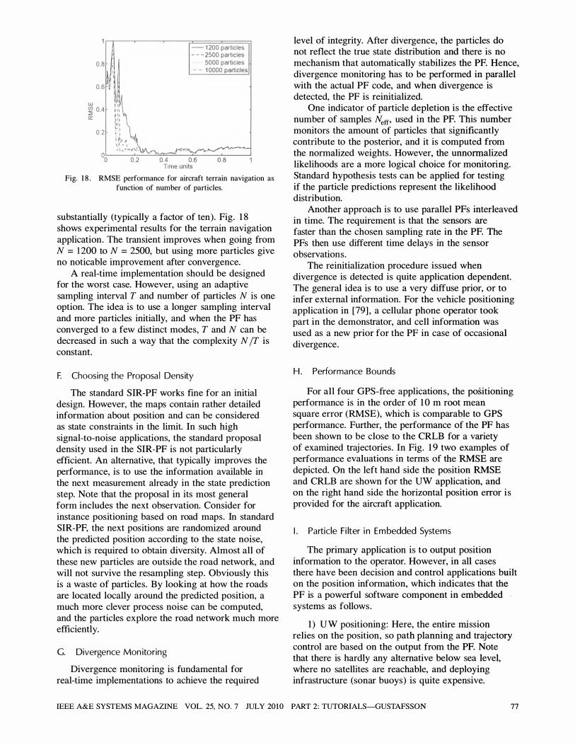
0.8

0.6

w � 0.4 n:

0 .2

- 1 200 particles - - - 2500 particles . . . . . . . 5000 particles ' - ' - , 1 0000 particles

Fig. 1 8 . RMSE performance for aircraft terrain navigation as

function of number of particles.

substantially (typically a factor of ten). Fig. 1 8 shows experimental results for the terrain navigation application. The transient improves when going from N = 1200 to N = 2500, but using more particles give no noticable improvement after convergence.

A real-time implementation should be designed for the worst case. However, using an adaptive sampling interval T and number of particles N is one option. The idea is to use a longer sampling interval and more particles initially, and when the PF has converged to a few distinct modes, T and N can be decreased in such a way that the complexity N IT is constant.

E Choos ing the Proposa l Dens ity

The standard SIR-PF works fine for an initial design. However, the maps contain rather detailed information about position and can be considered as state constraints in the limit. In such high signal-to-noise applications, the standard proposal density used in the SIR-PF is not particularly efficient. An alternative, that typically improves the performance, is to use the information available in the next measurement already in the state prediction step. Note that the proposal in its most general form includes the next observation. Consider for instance positioning based on road maps. In standard SIR-PF, the next positions are randomized around the predicted position according to the state noise, which is required to obtain diversity. Almost all of these new particles are outside the road network, and will not survive the resampling step. Obviously this is a waste of particles. By looking at how the roads are located locally around the predicted position, a much more clever process noise can be computed, and the particles explore the road network much more efficiently.

G. Divergence Mon itor ing

Divergence monitoring is fundamental for real-time implementations to achieve the required

level of integrity. After divergence, the particles do not reflect the true state distribution and there is no mechanism that automatically stabilizes the PF. Hence, divergence monitoring has to be performed in parallel with the actual PF code, and when divergence is detected, the PF is reinitialized.

One indicator of particle depletion is the effective number of samples Neff' used in the PF. This number monitors the amount of particles that significantly contribute to the posterior, and it is computed from the normalized weights . However, the unnormalized likelihoods are a more logical choice for monitoring. Standard hypothesis tests can be applied for testing if the particle predictions represent the likelihood distribution.

Another approach is to use parallel PFs interleaved in time. The requirement is that the sensors are faster than the chosen sampling rate in the PF. The PFs then use different time delays in the sensor observations.

The reinitialization procedure issued when divergence is detected is quite application dependent. The general idea is to use a very diffuse prior, or to infer external information. For the vehicle positioning application in [79] , a cellular phone operator took part in the demonstrator, and cell information was used as a new prior for the PF in case of occasional divergence.

H. Performance Bou nds

For all four GPS-free applications, the positioning performance is in the order of 1 0 m root mean square error (RMSE), which is comparable to GPS performance. Further, the performance of the PF has been shown to be close to the CRLB for a variety of examined trajectories. In Fig. 1 9 two examples of performance evaluations in terms of the RMSE are depicted. On the left hand side the position RMSE and CRLB are shown for the UW application, and on the right hand side the horizontal position error is provided for the aircraft application.

I . Particle F i lter i n E m bedded Systems

The primary application is to output position information to the operator. However, in all cases there have been decision and control applications built on the position information, which indicates that the PF is a powerful software component in embedded systems as follows.

1) UW positioning: Here, the entire mission relies on the position, so path planning and trajectory control are based on the output from the PF. Note that there is hardly any alternative below sea level, where no satellites are reachable, and deploying infrastructure (sonar buoys) is quite expensive.

IEEE A&E SYSTEMS MAGAZINE VOL. 25, NO. 7 JULY 2010 PART 2: TUTORIALS-GUSTAFSSON 77

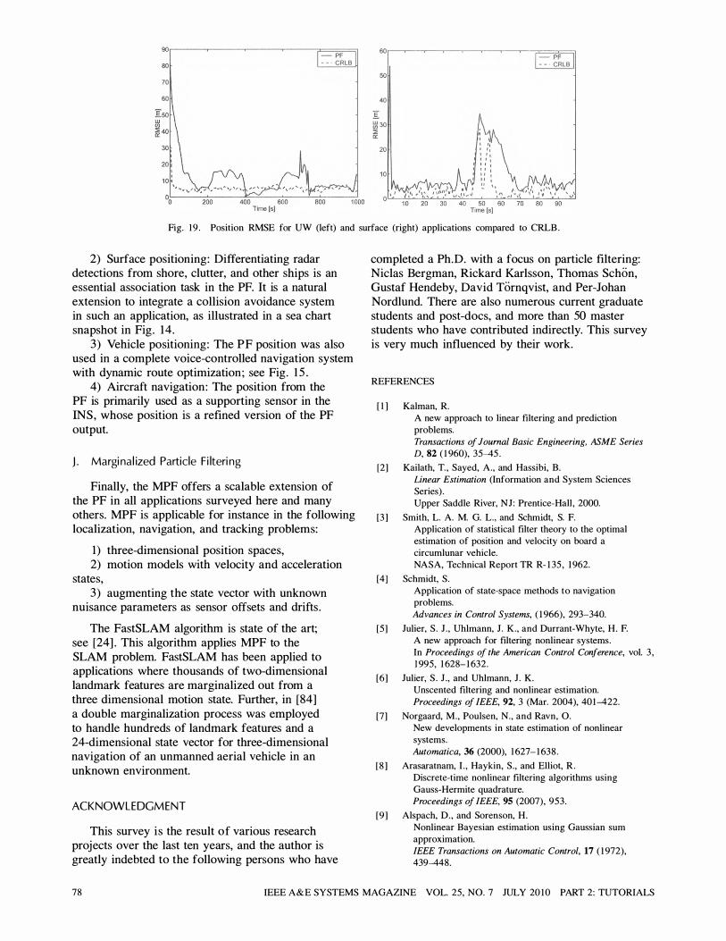
OO'---�----�----�----r=�P�F� 80 - _ . CRLB

70

60

6O'-��--��--��-'==�P�F� - - . CRLB

50

40

Fig. 19 . Position RMSE for UW (left) and surface (right) applications compared to CRLB .

2) Surface positioning: Differentiating radar detections from shore, clutter, and other ships is an essential association task in the PF. It is a natural extension to integrate a collision avoidance system in such an application, as illustrated in a sea chart snapshot in Fig. 14.

3) Vehicle positioning: The PF position was also used in a complete voice-controlled navigation system with dynamic route optimization; see Fig. 1 5 .

4) Aircraft navigation: The position from the PF is primarily used as a supporting sensor in the INS, whose position is a refined version of the PF output.

J . Margi nal ized Partic le F i lteri ng

Finally, the MPF offers a scalable extension of the PF in all applications surveyed here and many others. MPF is applicable for instance in the following localization, navigation, and tracking problems:

1) three-dimensional position spaces, 2) motion models with velocity and acceleration

states, 3) augmenting the state vector with unknown

nuisance parameters as sensor offsets and drifts.

The FastSLAM algorithm is state of the art; see [24] . This algorithm applies MPF to the SLAM problem. FastSLAM has been applied to applications where thousands of two-dimensional landmark features are marginalized out from a three dimensional motion state. Further, in [84] a double marginalization process was employed to handle hundreds of landmark features and a 24-dimensional state vector for three-dimensional navigation of an unmanned aerial vehicle in an unknown environment.

ACKNOWLEDGM ENT

This survey is the result of various research projects over the last ten years, and the author is greatly indebted to the following persons who have

completed a Ph.D. with a focus on particle filtering: Niclas Bergman, Rickard Karlsson, Thomas Schon, Gustaf Hendeby, David Tornqvist, and Per-Johan Nordlund. There are also numerous current graduate students and post-docs, and more than 50 master students who have contributed indirectly. This survey is very much influenced by their work.

REFERENCES

[ I ] Kalman, R.

A new approach to linear filtering and prediction

problems.

Transactions of Journal Basic Engineering, ASME Series D, 82 ( 1 960), 35-45 .

[2] Kailath, T. , Sayed, A., and Hassibi, B.

Linear Estimation (Information and System Sciences

Series) .

Upper Saddle River, NJ: Prentice-Hall , 2000.

[3 ] Smith, L. A. M. G. L., and Schmidt, S. F.

Application of statistical filter theory to the optimal

estimation of position and velocity on board a

circumlunar vehicle.

NASA, Technical Report TR R- 1 35 , 1 962.

[4] Schmidt, S .

Application of state-space methods to navigation

problems.

Advances in Control Systems, ( 1 966), 293-340.

[5] Julier, S . J . , Uhlmann, J. K., and Durrant-Whyte, H. F. A new approach for filtering nonlinear systems.

In Proceedings of the American Control Conference, vol. 3 ,

1 995, 1 628- 1 632.

[6] Julier, S . J . , and Uhlmann, J. K.

Unscented filtering and nonlinear estimation.

Proceedings of IEEE, 92, 3 (Mar. 2004), 401-422.

[7] Norgaard, M., Poulsen, N., and Ravn, O.

New developments in state estimation of nonlinear

systems.

Automatica, 36 (2000), 1 627- 1 638 .

[8 ] Arasaratnam, I . , Haykin, S. , and Elliot, R .

Discrete-time nonlinear filtering algorithms using

Gauss-Hermite quadrature.

Proceedings of IEEE, 95 (2007), 953.

[9] Alspach, D. , and Sorenson, H.

Nonlinear Bayesian estimation using Gaussian sum

approximation.

IEEE Transactions on Automatic Control, 17 ( 1 972),

439-448.


[ 1 0] Kramer, S . , and Sorenson, H. Recursive Bayesian estimation using piece-wise constant approximations. Automatica, 24 ( 1 988), 789-80 1 .

[ 1 1 ] Hammersley, J . , and Morton, K. Poor man' s Monte Carlo. Journal of the Royal Statistical Society, Series B, 16 ( 1 954), 23.

[ 1 2] Rosenbluth, M., and Rosenbluth, A. Monte Carlo calculation of the average extension of molecular chains. Journal of Chemical Physics, 23 ( 1 956), 590.

[ 1 3] Akashi, H., and Kumamoto, H. Random sampling approach to state estimation in switching environment. Automation, 13, 1 977, 429.

[ 1 4] Handshin, J. Monte Carlo techniques for prediction and filtering of nonlinear stochastic processes. Automatica, 6, 1 970, 555.

[ 1 5] Gordon, N., Salmond, D., and Smith, A. A novel approach to nonlinear/non-Gaussian Bayesian state estimation. In lEE Proceedings on Radar and Signal Processing, vol. 140, 1 993, 107-1 1 3 .

[ 1 6] Kitagawa, G. Monte Carlo filter and smoother for non-Gaussian nonlinear state space models. Journal of Computational and Graphical Statistics, S, 1 ( 1 996), 1-25 .

[ 1 7] Isard, M., and Blake, A. Condensation-Conditional density propagation for visual tracking. International Journal of Computer Vision, 29, 1 ( 1 998), 5-28.

[ 1 8] Doucet, A., de Freitas, N., and Gordon, N., (Eds.) Sequential Monte Carlo Methods in Practice. New York: Springer-Verlag, 200 1 .

[ 1 9] Liu, J. , and Chen, R. Sequential Monte Carlo methods for dynamic systems. Journal of the American Statistical Association, 93 ( 1 998).

[20] Arulampalam, S . , Maskell, S . , Gordon, N., and Clapp, T. A tutorial on particle filters for online nonlinear/non-Gaussian Bayesian tracking. IEEE Transactions on Signal Processing, 50, 2 (2002), 1 74-1 88 .

[2 1 ] Djuric, P., Kotecha, J. , Zhang, J . , Huang, Y., Ghirmai, T., Bugallo, M., and Miguez, J.

Particle filtering. IEEE Signal Processing Magazine, 20 (2003), 19 .

[22] Cappe, 0., Godsill, S., and Moulines, E. An overview of existing methods and recent advances in sequential Monte Carlo. IEEE Proceedings, 95 (2007), 899.

[23] Ristic, B., Arulampalam, S. , and Gordon, N. Beyond the Kalman filter: Particle filters for tracking applications. London: Artech House, 2004.

[24] Montemerlo, M., Thrun, S. , Koller, D. , and Wegbreit, B . FastSLAM a factored solution to the simultaneous localization and mapping problem. Presented at the AAAI National Conference on Artificial Intelligence, Edmonton, Canada, 2002.

[25] Durrant-Whyte, H. , and Bailey, T. Simultaneous localization and mapping (SLAM): Part I. IEEE Robotics & Automation Magazine, 13, 2 (June 2006), 99-1 10.

[26] Bailey, T. , and Durrant-Whyte, H. Simultaneous localization and mapping (SLAM): Part II. IEEE Robotics & Automation Magazine, 13, 3 (Sept. 2006), 108-1 17 .

[27] Thrun, S., Burgard, w., and Fox, D. Probabilistic Robotics. Cambridge, MA: MIT Press, 2005 .

[28] Rathi, Y., Vaswani, N., Tannenbaum, A., and Yezzi, A. Tracking deforming objects using particle filtering for geometric active contours. IEEE Transactions on Pattern Analysis and Machine Intelligence, 29, 8 (2007), 1470--1475.

[29] Rathi, Y., Vaswani, N., and Tannenbaum, A. A generic framework for tracking using particle filter with dynamic shape prior. IEEE Transactions on Image Processing, 16, 5 (2007), 1 370--1 382.

[30] Lu, W-L., Okuma, K., and Little, J. Tracking and recognizing actions of multiple hockey players using the boosted particle filter. Image and Vision Computing, 27 (2009), 1 89-205 .

[3 1 ] Cevher, V., Sankaranarayanan, A . , McClellan, J . , and Chellappa, R.

Target tracking using a joint acoustic video system. IEEE Transactions on Multimedia, 9, 4 (2007), 7 1 5-727.

[32] Bar-Shalom, Y., and Fortmann, T. Tracking and Data Association, vol. 179 (Mathematics in Science and Engineering Series). New York: Academic Press, 1 988 .

[33] Gustafsson, E, and Hendeby, G. On nonlinear transformations of stochastic variables and its application to nonlinear filtering. Presented at the IEEE International Conference on Acoustics, Speech, and Signal Processing, Las Vegas, NV, 2008.

[34] Gustafsson, E Adaptive Filtering and Change Detection. New York: Wiley, 200 1 .

[35] Jazwinsky, A. Stochastic Process and Filtering Theory, vol. 64 (Mathematics in Science and Engineering Series). New York: Academic Press, 1 970.

[36] Van Trees, H. Detection, Estimation and Modulation Theory. New York: Wiley, 1 97 1 .

[37] Robert, C. P., and Casella, G. Monte Carlo Statistical Methods, (Springer Texts in Statistics Series). New York: Springer, 1 999.

[38] Klaas, M. Toward practical n2 Monte Carlo: The marginal particle filter. Uncertainty in Artificial Intelligence, (2005).

[39] Poyiadjis, G., Doucet, A., and Singh, S. Maximum likelihood parameter estimation in general state-space models using particle methods. Presented at the Joint Statistical Meeting, Minneapolis, MN, 2005 .

[40] Poyiadjis, G., Doucet, A., and Singh, S . Maximum likelihood parameter estimation using particle methods. Presented at the IEEE Conference on Acoustics, Speech and Signal Processing, 2006.

[4 1 ] Martinez-Cantin, R., de Freitas, N., and Castellanos, J. Analysis of particle methods for simultaneous robot localization and mapping and a new algorithm: Marginal-slam. Presented at the IEEE International Conference on Robotics and Automation, Rome, Italy, 2007 .


[42] Sing, S., Kantas, N., Yo, B . , Doucet, A., and Evans, R Simulation-based optimal sensor scheduling with application to observer trajectory planning. Automatica, 43 (2007), 8 1 7-830.

[43] Doucet, A., Godsill, S . , and Andrieu, C. On sequential simulation-based methods for Bayesian filtering. Statistics and Computing, 10, 3 (2000), 1 97-208.

[44] Kotecha, J., and Djuric, P. Gaussian particle filtering. IEEE Transactions on Signal Processing, 51 (2003), 2592.

[45] Kotecha, J. , and Djuric, P. Gaussian sum particle filtering. IEEE Transactions on Signal Processing, 51 (2003), 2602.

[46] Kong, A., Liu, J. S. , and Wong, W. H. Sequential imputations and Bayesian missing data problems. Journal of American Statistical Association, 89, 425 ( 1 994), 278-288.

[47] Liu, J. Metropolized independent sampling with comparison to rejection sampling and importance sampling. Statistics and Computing, 6 ( 1 996), 1 1 3-1 1 9.

[48] Fearnhead, P. Sequential Monte Carlo methods in filter theory. Ph.D. dissertation, University of Oxford, UK, 1998.

[49] Doucet, A., Gordon, N., and Krishnamurthy, V. Particle filters for state estimation of jump Markov linear systems. IEEE Transactions on Signal Processing, 49, 3 (2001) , 6 1 3-624.

[50] Pitt, M., and Shephard, N. Filtering via simulation: Auxiliary particle filters. Journal of the American Statistical Association, 94, 446 (June 1 999), 590-599

[5 1 ] Doucet, A, Briers, M., and Senecal, S . Efficient block sampling strategies for sequential Monte Carlo methods. Journal of Computational and Graphical Statistics, 15, 3 (2006), 1-19 .

[52] Thrun, S., Fox, D., Dellaert, F. , and Burgard, W. Particle filters for mobile robot localization. In A. Doucet, N. de Freitas, and N. Gordon, (Eds.), Sequential Monte Carlo Methods in Practice, New York: Springer-Verlag, 200 1 .

[53] Johansen, A., and Doucet, A A note on auxiliary particle filters. Statistics & Probability Letters, 78, 12 (2008), 1498-1 504.

[54] Crisan, D., and Doucet, A. Convergence of sequential Monte Carlo methods. Signal Processing Group, Department of Engineering, University of Cambridge, Technical Report CUEDIF-INFENGrrR38 1 , 2000.

[55] Moral, P. D. Feynman-Kac Formulae: Genealogical and Interacting Particle Systems with Applications. New York: Springer, 2004.

[56] Crisan, D., and Doucet, A. A survey of convergence results on particle filtering methods for practitioners. IEEE Transactions on Signal Processing, 50, 3 (2002), 736-746.

[57] Hu, X., Schon, T. , and Ljung, L. A basic convergence result for particle filtering. IEEE Transactions on Signal Processing, 56, 4 (Apr. 2008), 1 337- 1 348.

[58] Hendeby, G. Performance and implementation aspects of nonlinear filtering. Dissertation No. 1 1 6 1 , Linkoping University, Sweden, 2008.

[59] Bergman, A D. N., and Gordon, N. Optimal estimation and Cramer-Rao bounds for partial non-Gaussian state-space model. Annals of the Institute of Statistical Mathematics, 52, 1 (200 1 ), 97-1 12 .

[60] Ripley, B . Stochastic Simulation. Hoboken, NJ: Wiley, 1988.

[61 ] Velmurugan, R, Subramanian, S . , Cevher, V., Abramson, D. , Odame, K., Gray, J . , Lo, H-J., McClellan, M., and Anderson, D.

On low-power analog implementation of particle filters for target tracking. In Proceedings of the European Signal Processing Conference (EUSIPCO), 2006.

[62] Coppersmith, D., and Winograd, S. Matrix multiplication via arithmetic progressions. Journal of Symbolic Computation, 9 ( 1 990), 25 1 -280.

[63] Doucet, A., Godsill, S . J. , and Andrieu, C. On sequential Monte Carlo sampling methods for Bayesian filtering. Statistics and Computing, 10, 3 (2000), 1 97-208.

[64] Casella, G., and Robert, C. P. Rao-Blackwellisation of sampling schemes. Biometrika, 83, 1 ( 1 996), 8 1-94.

[65] Chen, R, and Liu, J. S. Mixture Kalman filters. Journal of the Royal Statistical Society, 62, 3 (2000), 493-508.

[66] Andrieu, C. , and Doucet, A Particle filtering for partially observed Gaussian state space models. Journal of the Royal Statistical Society, 64, 4 (2002), 827-836.

[67] Schon, T. , Gustafsson, F. , and Nordlund, P. Marginalized particle filters for nonlinear state-space models. IEEE Transactions on Signal Processing, 53 (2005), 2279-2289.

[68] Nordlund, P-J. , and Gustafsson, F. Marginalized particle filter for accurate and reliable terrain-aided navigation. IEEE Transactions on Aerospace and Electronic Systems, 35, 3 (2008).

[69] Hendeby, G., Karlsson, R., and Gustafsson, F. A new formulation of the Rao-Blackwellized particle filter. In Proceedings of IEEE Workshop on Statistical Signal Processing, Madison, WI, Aug. 2007.

[70] Karlsson, R., Schon, T. , and Gustafsson, F. Complexity analysis of the marginalized particle filter. IEEE Transactions on Signal Processing, 53 (2005), 4408-44 1 1 .

[7 1 ] Simandl, M., Knilovec, J . , and Soderstrom, T. Advanced point-mass method for nonlinear state estimation. Automatica, 42, 7 (July 2006), 1 1 33-1 145.

[72] Gustafsson, F., Gunnarsson, F., Bergman, N., Forssell, U., Jansson, J. , Karlsson, R, and Nordlund, P-J .

Particle filters for positioning, navigation and tracking. IEEE Transactions on Signal Processing, 50, 2 (Feb. 2002), 425-437.


[73] Karlsson, R., and Gustafsson, F. Bayesian surface and underwater navigation.

[79] Forssell, U., Hall, P., Ahlqvist, S., and Gustafsson, F. Novel map-aided positioning system.

IEEE Transactions on Signal Processing, 54, 1 1 (2006), 4204-42 1 3 .

I n Proceedings of FISITA , no. F02- 1 1 3 1 , Helsinki, 2002. [80] Hall, P.

[74] Fauske, K., Gustafsson, F., and Herenaes, O. Estimation of AUV dynamics for sensor fusion. In Proceedings of Fusion 2007, Quebec, Canada, July, 2007.

A Bayesian approach to map-aided vehicle positioning. Department of Electric Engineering, Linkoping University, S-5 8 1 83 Linkoping, Sweden, Master' s Thesis LiTH-ISY-EX-3 104, 200 1 , in Swedish.

[75] Karlsson, T. Terrain aided underwater navigation using Bayesian statistics.

[8 1 ] Kronander, J. Robust vehicle positioning: Integration of GPS and motion sensors.

Department of Electrical Engineering, Linkoping University, S-5 8 1 83, Linkoping, Sweden, Master' s Thesis LiTH-ISY-EX-3292, 2002.

Department of Electrical Engineering, Linkoping University, S-5 8 1 83 Linkoping, Sweden, Master' s Thesis LiTH-ISY-EX-3578, 2003 .

[76] Dahlin, M., and Mahl, S. [82] Athalye, A. Radar distance positioning system-With a particle filter approach.

Design and implementation of reconfigurable hardware for real-time particle filtering.

Department of Electrical Engineering, Linkoping University, Master' s Thesis LiTH-ISY EX-3998.

Ph.D. dissertation, Stody Brook University, 2007. [83] Hendeby, G. , Hoi, J. D. , Karlsson, R., and Gustafsson, F.

[77] Ronnebjerg, A. A tracking and collision warning system for maritime applications.

A graphics processing unit implementation of the particle filter.

Department of Electrical Engineering, Linkoping University, S-58 1 83 Linkoping, Sweden, Master' s Thesis LiTH-ISY-EX-3709, 2005, in Swedish.

[78] Lo, S., Peterson, 8., and Enge, P.

In Proceedings of the European Signal Processing Conference (EUSIPCO), Pozna'n, Poland, Sept. 2007.

[84] Karlsson, R., Schon, T. , Tornqvist, D., Conte, G., and Gustafsson, F.

Utilizing model structure for efficient simultaneous localization and mapping for a UAV application. Loran data modulation: A primer (AESS Tutorial IV).

IEEE Aerospace and Electronic Systems Magazine, 22 (2007), 3 1-5 1 .

In Proceedings of IEEE Aerospace Conference, Big Sky, MT, 2008.

Fredrik Gustafsson received the M.Sc. degree in electrical engineering 1 988 and the Ph.D. degree in automatic control, 1 992, both from Linkoping University.

During 1 992-1999 he held various positions in automatic control, and 1 999-2005 he had a professorship in communication systems. He has been a professor in the Sensor Informatics at Department of Electrical Engineering, Linkoping University, since 2005 . His research interests are in stochastic signal processing, adaptive filtering, and change detection, with applications to communication, vehicular, airborne, and audio systems. His work in the sensor fusion area involves design and implementation of nonlinear filtering algorithms for localization, navigation and tracking of all kind of platforms, including cars, aircraft, spacecraft, UAV s, surface and underwater vessels, cell phones, and film cameras for augmented reality. He is a cofounder of the companies NIRA Dynamics and Softube, developing signal processing software solutions for automotive and music industry, respectively.

He was an associate editor for IEEE Transactions of Signal Processing 2000-2006 and is currently associate editor for EURASIP Journal on Applied Signal Processing and International Journal of Navigation and Observation. In 2004, he was awarded the Amberg prize by the Royal Swedish Academy of Science (KVA) and in 2007 he was elected member of the Royal Academy of Engineering Sciences (IVA) .

IEEE A&E SYSTEMS MAGAZINE VOL. 25, NO. 7 JULY 201 0 PART 2: TUTORIALS-GUSTAFSSON 8 1

Particle Filter Theory and Practice with Positioning …360880/FULLTEXT… · ·...

Documents

Transcript of Particle Filter Theory and Practice with Positioning …360880/FULLTEXT… · ·...