Mon. Not. R. Astron. Soc. 000, 1–16 (2014) Printed 13 August 2018 (MN LATEX style file v2.2)

Particle acceleration in axisymmetric pulsar current sheets

Benoıt Cerutti?†, Alexander Philippov, Kyle Parfrey and Anatoly SpitkovskyDepartment of Astrophysical Sciences, Princeton University, Princeton, NJ 08544, USA.

Accepted –. Received –; in original form –

ABSTRACTThe equatorial current sheet in pulsar magnetospheres is often regarded as an idealsite for particle acceleration via relativistic reconnection. Using 2D spherical particle-in-cell simulations, we investigate particle acceleration in the axisymmetric pulsarmagnetosphere as a function of the injected plasma multiplicity and magnetization.We observe a clear transition from a highly charge-separated magnetosphere for lowplasma injection with little current and spin-down power, to a nearly force-free solutionfor high plasma multiplicity characterized by a prominent equatorial current sheet andhigh spin-down power. We find significant magnetic dissipation in the current sheet,up to 30% within 5 light-cylinder radii in the high-multiplicity regime. The simulationsunambiguously demonstrate that the dissipated Poynting flux is efficiently channeledto the particles in the sheet, close to the Y-point within about 1-2 light cylinderradii from the star. The mean particle energy in the sheet is given by the upstreamplasma magnetization at the light cylinder. The study of particle orbits shows that allenergetic particles originate from the boundary layer between the open and the closedfield lines. Energetic positrons always stream outward, while high-energy electronsprecipitate back towards the star through the sheet and along the separatrices, whichmay result in auroral-like emission. Our results suggest that the current sheet and theseparatrices may be the main source of high-energy radiation in young pulsars.

Key words: acceleration of particles – magnetic reconnection – methods: numerical– pulsars: general – stars: winds, outflows.

1 INTRODUCTION

Young pulsars represent the majority of the high-energygamma-ray sources identified in our Galaxy (Abdo et al.2013). In spite of exquisite data, the origin of the gamma-ray emission remains poorly understood. The high-energygamma rays are often associated with curvature radiation,emitted by relativistic electron-positron pairs accelerated intiny regions where the electric field is not perfectly screenedby the plasma (the so-called “gap” models, e.g., Arons 1983;Cheng et al. 1986; Romani 1996; Muslimov & Harding 2003).In this framework, particle acceleration and emission areconfined within the corotating magnetosphere delimited bythe light cylinder of radius RLC = Pc/2π, where P is thespin period of the star and c is the speed of light.

There has been significant progress in the numericalmodeling of pulsar magnetospheres, mostly in the magneto-hydrodynamic (MHD) limit (force-free, resistive force-free,and full MHD, see e.g., Contopoulos et al. 1999; Gruzinov2005; Komissarov 2006; Spitkovsky 2006; McKinney 2006;Timokhin 2006; Kalapotharakos & Contopoulos 2009; Bai

? E-mail: bcerutti@astro.princeton.edu† Lyman Spitzer Jr. Fellow.

& Spitkovsky 2010; Kalapotharakos et al. 2012; Petri 2012b;Parfrey et al. 2012; Li et al. 2012; Tchekhovskoy et al. 2013),and most recently using particle-in-cell (PIC) simulations(Philippov & Spitkovsky 2014; Chen & Beloborodov 2014).A prominent feature found in these simulations is the pres-ence of strong current sheets in the magnetosphere. Onecurrent sheet forms near the star in each hemisphere atthe boundary between the open and the closed field lines(or separatrix). Both sheets merge at the end of the closedzone near the light-cylinder radius (at the “Y-point”), andcreate a single current layer which supports open magneticfield lines. Coroniti (1990) proposed that dissipation in thecurrent sheet via relativistic reconnection could account forthe efficient transfer of magnetic flux into energetic parti-cles (i.e., the “sigma-problem”). Lyubarskii (1996) pointedout that the observed pulsed gamma-ray emission could be anatural outcome of such a process. In this scenario, particlesare accelerated in the current sheet and radiate synchrotrongamma-ray photons (Kirk et al. 2002; Petri 2012a; Arka &Dubus 2013; Uzdensky & Spitkovsky 2014).

PIC simulations of isolated current sheets show thatrelativistic reconnection in collisionless pair plasmas isfast and efficient at accelerating particles (e.g., Zenitani &Hoshino 2001; Jaroschek et al. 2004; Cerutti et al. 2014;

c© 2014 RAS

arX

iv:1

410.

3757

v2 [

astr

o-ph

.HE

] 7

Jan

201

5

2 Benoıt Cerutti et al.

Sironi & Spitkovsky 2014; Guo et al. 2014; Werner et al.2014). However, there are important differences betweenthese local simulations and the global structure of thecurrent sheet in pulsars (e.g., geometrical effects, gradients,strong electric field induced by the rotation of the star,absorption/creation of particles), so the results might notbe directly applicable. The first kinetic simulations of thealigned pulsar show that the current layers are indeedinvolved in particle acceleration (Philippov & Spitkovsky2014; Chen & Beloborodov 2014), but the details of theacceleration mechanism remains unclear.

In this paper, we present a comprehensive analysis ofparticle acceleration in the aligned pulsar magnetosphereusing large, high-resolution two-dimensional (2D) axisym-metric PIC simulations. In addition, this work explores theeffect of the plasma supply and magnetization on the globalstructure of the magnetosphere, and on the pulsar spin-downpower. This article is organized as follows. In Sect. 2 we de-scribe the implementation of the 2D spherical axisymmetricgrid in the Zeltron code. Most of the technical details aregiven in the appendices (Appendix A, B). We describe howthe simulation is set up, with a particular emphasis on theboundary conditions. In Sect. 3 we present the main resultsof this study, which are summarized in Sect. 4.

2 NUMERICAL TOOLS AND SETUP

2.1 The Zeltron code in spherical coordinates

In this study, we use the explicit, massively parallel, electro-magnetic PIC code Zeltron, initially developed for relativis-tic reconnection studies (Cerutti et al. 2013, 2014). The codeemploys the standard second-order accurate Yee algorithm(Yee 1966) to advance the electromagnetic field in time, andthe second-order accurate Boris (Birdsall & Langdon 1991)or Vay (2008) algorithms to solve the equation of motionof the particles. Zeltron does not follow a strictly charge-conserving scheme, instead small errors accumulated in theelectric field are corrected periodically by solving Poisson’sequation (Pritchett 2003). To perform simulations of thealigned pulsar, we implemented a 2D axisymmetric spher-ical grid in Zeltron (see also the recent developments byChen & Beloborodov 2014 and Belyaev 2015). Maxwell’sequations are discretized and solved on the spherical Yeemesh, using the formulae given in Appendix A, while theparticles’ equations of motion are solved in Cartesian coor-dinates. The positions and velocities of the particles are thenremapped onto the spherical grid where their charges andcurrents are deposited using the volume weighting technique(bilinear interpolation in r3 and cos θ) given in Appendix B.As discussed below, using spherical coordinates greatly sim-plifies the formulation of the boundary conditions.

2.2 The grid

The computational domain extends in radius from the sur-face of the star, i.e., r = r?, up to r = rmax = 6.67RLC,and from θ = 0 to θ = 180 (see Fig. 1). The light-cylinderradius is set at RLC = 3r?. The spin axis of the star isaligned along θ = 0. The grid points are uniformly spaced

r⋆

rabs

rmax

Dipole

Absorbing layer (λE, λ⋆B)

Reflecting wall

Axial symmetry:

Log-spherical grid

RLC

Ω

Open: ∂(E,B)∂r = 0

∂(E,B)r∂θ = 0, (E,B)θ,φ = 0

Injection of cold pairs

Br, Eθ, Eφ fixed

∆r

Vacuum

along field lines

φ

rθ

Light cylinder

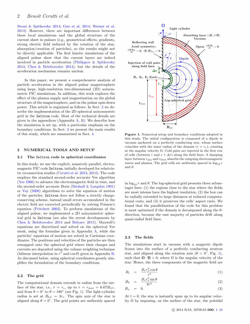
Figure 1. Numerical setup and boundary conditions adopted in

this study. The initial configuration is composed of a dipole invacuum anchored on a perfectly conducting star, whose surface

coincides with the inner radius of the domain (r = r?), rotatingat the angular velocity Ω. Cold pairs are injected in the first row

of cells (between r and r + ∆r) along the field lines. A damping

layer between rabs and rmax absorbs the outgoing electromagneticwaves and plasma. The grid cells are uniformly spaced in log10 r

and θ.

in log10 r and θ. The log-spherical grid presents three advan-tages here: (1) the regions close to the star where the fieldsare most intense have the highest resolution, (2) the box canbe radially extended to large distances at reduced computa-tional costs, and (3) it preserves the cells’ aspect ratio. Wefound that the parallelization of the code for this problemis most optimized if the domain is decomposed along the θ-direction, because the vast majority of particles drift alongquasi-radial field lines.

2.3 The fields

The simulations start in vacuum with a magnetic dipolefrozen into the surface of a perfectly conducting neutronstar, and aligned along the rotation axis (θ = 0, Fig. 1),such that Ω ·B > 0, where Ω is the angular velocity of thestar. Hence, the three components of the magnetic field are

Br =B?r

3? cos θ

r3(1)

Bθ =B?r

3? sin θ

2r3(2)

Bφ = 0. (3)

At t = 0, the star is instantly spun up to its angular veloc-ity Ω by imposing, on the surface of the star, the poloidal

c© 2014 RAS, MNRAS 000, 1–16

Particle acceleration in axisymmetric pulsar current sheets 3

electric field induced by the rotation of the field lines

Eθ(r?, θ) = − (Ω×R)×Br

c

= −r? sin θ

RLCBr(r?, θ)eθ, (4)

where R = r sin θ is the cylindrical radius, and where eθ isthe unit vector in the θ-directions. The toroidal electric fieldat the surface of the star is set to Eφ(r?, θ) = 0 at all times.

The choice of the outer boundary condition for the fieldsis more involved. To mimic an open boundary in which noinformation is able to come back inward, we define an ab-sorbing layer starting at r = rabs and extending to the endof the box, where Maxwell’s equations contain an electricand a magnetic conductivity terms (see red shaded regionin Fig. 1), such that (Birdsall & Langdon 1991)

∂E

∂t= −λ(r)E + c (∇×B)− 4πJ (5)

∂B

∂t= −λ?(r)B− c (∇×E) . (6)

One can avoid undesirable reflections of waves at r = rabs bygradually increasing the conductivities with distance. Em-pirically, we found that the following conductivity profile isa good damping layer,

λ(r) = λ?(r) =Kabs

∆t

(r − rabs

rmax − rabs

)3

, if r > rabs (7)

λ(r) = λ?(r) = 0, otherwise, (8)

where ∆t is the time step (see its definition in Appendix A),and Kabs > 1 is a numerical parameter that controls thedamping strength. Here, we choose Kabs = 40. At r =rmax, we apply a zero gradient condition on the fields, i.e.,∂E/∂r = 0 and ∂B/∂r = 0. The absorbing layer is set atrabs = 0.9rmax in all the simulations presented here.

Thanks to the integral form of Maxwell’s equations de-rived in Appendix A, we are able to push the θ-boundariesto the axis (there is no division by sin θ). Then one can sim-ply apply the axial symmetry to the fields at θ = 0 andθ = π: Eθ,φ = 0, Bθ,φ = 0 and ∂Er/∂θ = 0, ∂Br/∂θ = 0.

2.4 The particles

In principle, one should model the full electromagnetic cas-cade to obtain a self-consistent injection of pairs into themagnetosphere (e.g., Timokhin & Arons 2013; Chen & Be-loborodov 2014). Instead of solving for the cascade, we pro-pose a simple and robust way to fill the magnetosphere withplasma. This method consists of injecting a neutral plasmaof pairs at every time step uniformly between the surfaceof the neutron star r? and r? + ∆r, where ∆r is the thick-ness of the first row of cell along the r-direction, and withno angular dependence. The particles are injected along thefield lines with a poloidal velocity, vpol = 0.5c, and in coro-tation with the star, i.e., with vφ = RΩ. The flux of particlesinjected at every time step is

Finj = vpolfinjn?GJ, (9)

where n?GJ = B?/(2πRLCe) is the Goldreich-Julian density(Goldreich & Julian 1969) at the pole of the star. Thisconfiguration mimics the injection of fresh plasma by the

cascade everywhere close to the star. The efficiency of thecascade is parametrized by the injection rate finj. Eventhough the injection rate of particles per time step is fixed,the plasma density at the surface of the star is free tovary with time and θ, depending on the amount of plasmatrapped near the surface and the number of particles return-ing back to the star. However, to avoid over-injecting intothe closed zone where the plasma is trapped, the code addsnew pairs only if the plasma at the surface of the star iswell magnetized. Plasma magnetization is quantified by theσ-parameter, defined here as

σ ≡ B2

4πΓ(n+ + n−)mec2(10)

where (n+ + n−) is the total plasma density, and Γ is theplasma bulk Lorentz factor. We define a minimum value forσ at the surface of the star, σ? ≡ σ(r?) 1, below whichno pairs are injected.

To model the special case of a “dead” pulsar where thereis no pair production, i.e., the “electrosphere” or the “disk-dome” solution (see review by Michel & Li 1999), we useda slightly different method. In this case, the amount of newinjected charges is controlled by the surface charge density,Σ, given by the jump condition

4πΣ = Er(r?)− Ecor (r?), (11)

where Er(r?) is the radial electric field at the surface of thestar, while Eco

r (r?) = −(Ω×R)×Bθ/c is the radial corotat-ing electric field at r = r?. If Σ < 0 (Σ > 0), only electrons(positrons) are injected with the appropriate density, andwithout any initial velocity along the field lines, i.e., vpol = 0.In practice, we release only a fraction of Σ (a few percent)every time step, to avoid over-injection. The code stops in-jecting new particles when the density of charge reaches theGoldreich-Julian charge density, ρGJ = −(Ω ·B)/2πc.

Regardless of the injection method, any particle thatstrikes the r = r? boundary is removed from the simulation.The same fate applies to any particle leaving the workingdomain into the absorbing layer, i.e., if r > rabs. Our resultsare unchanged if the particles are removed further out, atr = rmax. On the axis, particles are reflected with no loss ofenergy.

2.5 Physical and numerical parameters

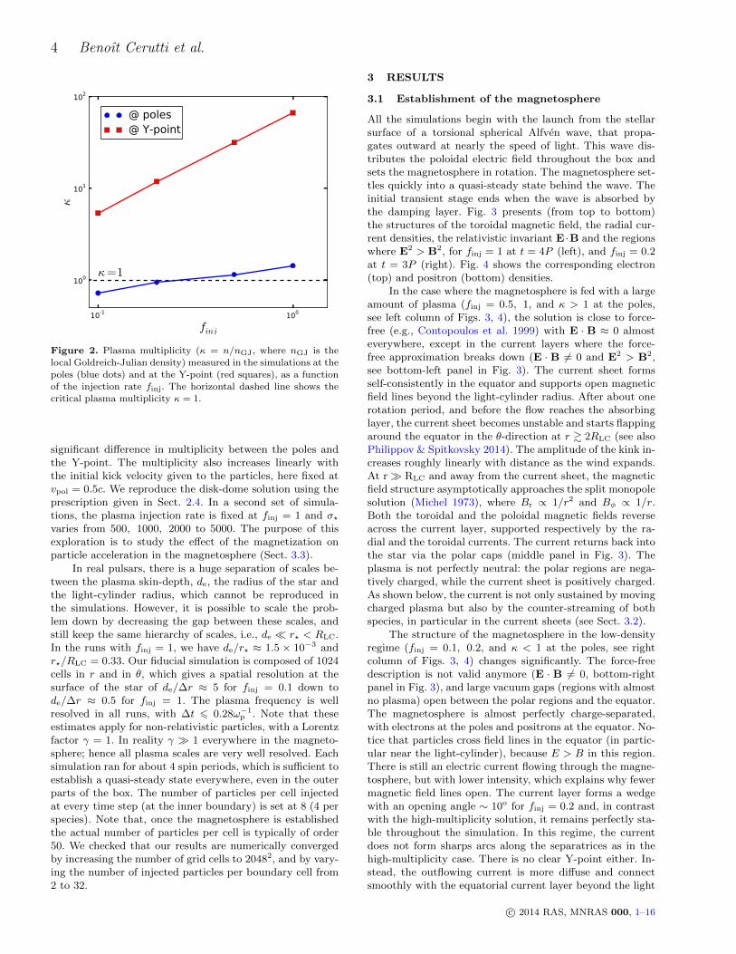
We perform a series of simulations in which we vary theplasma injection rate finj, and the minimum plasma mag-netization parameter defined at the star’s surface, σ?. Inthe first set we keep σ? = 5000 fixed, and study the tran-sition between a charge-starved magnetosphere for finj 1where pair production is inefficient, to a force-free mag-netosphere filled with a dense plasma for finj = 1 whereE · B = 0 everywhere (except in the current sheet). Theforce-free regime is appropriate to describe young gamma-ray pulsars which are characterized by intense surface mag-netic fields, B? ∼ 1012 G, and very large plasma multiplici-ties κ 1. The multiplicity is defined as the ratio betweenthe plasma density and the local Goldreich-Julian plasmadensity nGJ = |Ω · B|/2πec. Fig. 2 shows the actual lo-cal plasma multiplicities achieved in each simulation at thepoles and at the Y-point, as a function of finj. The multiplic-ity increases approximatively linearly with finj. Notice the

c© 2014 RAS, MNRAS 000, 1–16

4 Benoıt Cerutti et al.

10-1 100

finj

100

101

102

κ

κ=1

@ poles@ Y-point

Figure 2. Plasma multiplicity (κ = n/nGJ, where nGJ is the

local Goldreich-Julian density) measured in the simulations at the

poles (blue dots) and at the Y-point (red squares), as a functionof the injection rate finj. The horizontal dashed line shows the

critical plasma multiplicity κ = 1.

significant difference in multiplicity between the poles andthe Y-point. The multiplicity also increases linearly withthe initial kick velocity given to the particles, here fixed atvpol = 0.5c. We reproduce the disk-dome solution using theprescription given in Sect. 2.4. In a second set of simula-tions, the plasma injection rate is fixed at finj = 1 and σ?varies from 500, 1000, 2000 to 5000. The purpose of thisexploration is to study the effect of the magnetization onparticle acceleration in the magnetosphere (Sect. 3.3).

In real pulsars, there is a huge separation of scales be-tween the plasma skin-depth, de, the radius of the star andthe light-cylinder radius, which cannot be reproduced inthe simulations. However, it is possible to scale the prob-lem down by decreasing the gap between these scales, andstill keep the same hierarchy of scales, i.e., de r? < RLC.In the runs with finj = 1, we have de/r? ≈ 1.5 × 10−3 andr?/RLC = 0.33. Our fiducial simulation is composed of 1024cells in r and in θ, which gives a spatial resolution at thesurface of the star of de/∆r ≈ 5 for finj = 0.1 down tode/∆r ≈ 0.5 for finj = 1. The plasma frequency is wellresolved in all runs, with ∆t 6 0.28ω−1

p . Note that theseestimates apply for non-relativistic particles, with a Lorentzfactor γ = 1. In reality γ 1 everywhere in the magneto-sphere; hence all plasma scales are very well resolved. Eachsimulation ran for about 4 spin periods, which is sufficient toestablish a quasi-steady state everywhere, even in the outerparts of the box. The number of particles per cell injectedat every time step (at the inner boundary) is set at 8 (4 perspecies). Note that, once the magnetosphere is establishedthe actual number of particles per cell is typically of order50. We checked that our results are numerically convergedby increasing the number of grid cells to 20482, and by vary-ing the number of injected particles per boundary cell from2 to 32.

3 RESULTS

3.1 Establishment of the magnetosphere

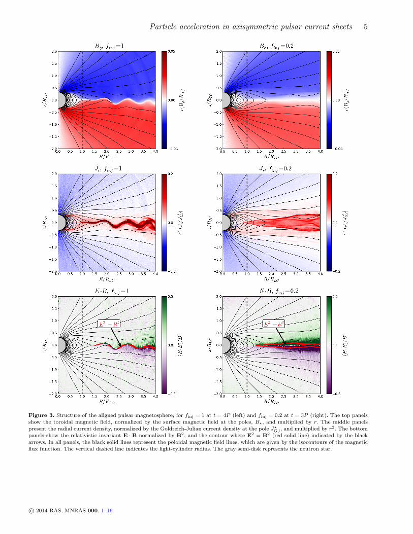
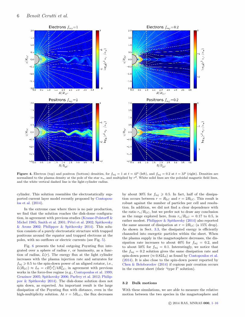
All the simulations begin with the launch from the stellarsurface of a torsional spherical Alfven wave, that propa-gates outward at nearly the speed of light. This wave dis-tributes the poloidal electric field throughout the box andsets the magnetosphere in rotation. The magnetosphere set-tles quickly into a quasi-steady state behind the wave. Theinitial transient stage ends when the wave is absorbed bythe damping layer. Fig. 3 presents (from top to bottom)the structures of the toroidal magnetic field, the radial cur-rent densities, the relativistic invariant E ·B and the regionswhere E2 > B2, for finj = 1 at t = 4P (left), and finj = 0.2at t = 3P (right). Fig. 4 shows the corresponding electron(top) and positron (bottom) densities.

In the case where the magnetosphere is fed with a largeamount of plasma (finj = 0.5, 1, and κ > 1 at the poles,see left column of Figs. 3, 4), the solution is close to force-free (e.g., Contopoulos et al. 1999) with E · B ≈ 0 almosteverywhere, except in the current layers where the force-free approximation breaks down (E · B 6= 0 and E2 > B2,see bottom-left panel in Fig. 3). The current sheet formsself-consistently in the equator and supports open magneticfield lines beyond the light-cylinder radius. After about onerotation period, and before the flow reaches the absorbinglayer, the current sheet becomes unstable and starts flappingaround the equator in the θ-direction at r & 2RLC (see alsoPhilippov & Spitkovsky 2014). The amplitude of the kink in-creases roughly linearly with distance as the wind expands.At r RLC and away from the current sheet, the magneticfield structure asymptotically approaches the split monopolesolution (Michel 1973), where Br ∝ 1/r2 and Bφ ∝ 1/r.Both the toroidal and the poloidal magnetic fields reverseacross the current layer, supported respectively by the ra-dial and the toroidal currents. The current returns back intothe star via the polar caps (middle panel in Fig. 3). Theplasma is not perfectly neutral: the polar regions are nega-tively charged, while the current sheet is positively charged.As shown below, the current is not only sustained by movingcharged plasma but also by the counter-streaming of bothspecies, in particular in the current sheets (see Sect. 3.2).

The structure of the magnetosphere in the low-densityregime (finj = 0.1, 0.2, and κ < 1 at the poles, see rightcolumn of Figs. 3, 4) changes significantly. The force-freedescription is not valid anymore (E · B 6= 0, bottom-rightpanel in Fig. 3), and large vacuum gaps (regions with almostno plasma) open between the polar regions and the equator.The magnetosphere is almost perfectly charge-separated,with electrons at the poles and positrons at the equator. No-tice that particles cross field lines in the equator (in partic-ular near the light-cylinder), because E > B in this region.There is still an electric current flowing through the magne-tosphere, but with lower intensity, which explains why fewermagnetic field lines open. The current layer forms a wedgewith an opening angle ∼ 10o for finj = 0.2 and, in contrastwith the high-multiplicity solution, it remains perfectly sta-ble throughout the simulation. In this regime, the currentdoes not form sharps arcs along the separatrices as in thehigh-multiplicity case. There is no clear Y-point either. In-stead, the outflowing current is more diffuse and connectsmoothly with the equatorial current layer beyond the light

c© 2014 RAS, MNRAS 000, 1–16

Particle acceleration in axisymmetric pulsar current sheets 5

Figure 3. Structure of the aligned pulsar magnetosphere, for finj = 1 at t = 4P (left) and finj = 0.2 at t = 3P (right). The top panels

show the toroidal magnetic field, normalized by the surface magnetic field at the poles, B?, and multiplied by r. The middle panelspresent the radial current density, normalized by the Goldreich-Julian current density at the pole J?GJ, and multiplied by r2. The bottom

panels show the relativistic invariant E · B normalized by B2, and the contour where E2 = B2 (red solid line) indicated by the black

arrows. In all panels, the black solid lines represent the poloidal magnetic field lines, which are given by the isocontours of the magneticflux function. The vertical dashed line indicates the light-cylinder radius. The gray semi-disk represents the neutron star.

c© 2014 RAS, MNRAS 000, 1–16

6 Benoıt Cerutti et al.

Figure 4. Electron (top) and positron (bottom) densities, for finj = 1 at t = 4P (left), and finj = 0.2 at t = 3P (right). Densities arenormalized to the plasma density at the pole of the star n?, and multiplied by r2. White solid lines are the poloidal magnetic field lines,

and the white vertical dashed line is the light-cylinder radius.

cylinder. This solution resembles the electrostatically sup-ported current layer model recently proposed by Contopou-los et al. (2014).

In the extreme case where there is no pair production,we find that the solution reaches the disk-dome configura-tion, in agreement with previous studies (Krause-Polstorff &Michel 1985; Smith et al. 2001; Petri et al. 2002; Spitkovsky& Arons 2002; Philippov & Spitkovsky 2014). This solu-tion consists of a purely electrostatic structure with trappedpositrons around the equator and trapped electrons at thepoles, with no outflows or electric currents (see Fig. 5).

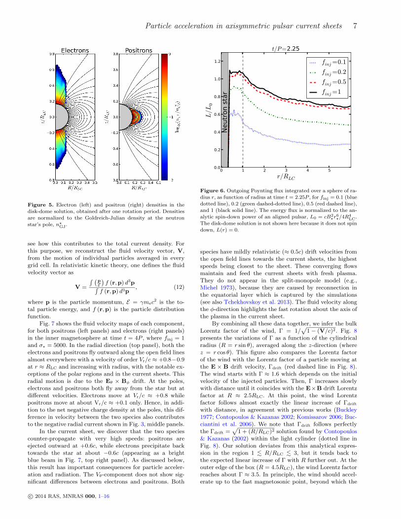
Fig. 6 presents the total outgoing Poynting flux inte-grated over a sphere of radius r, or luminosity, as a func-tion of radius, L(r). The energy flux at the light cylinderincreases with the plasma injection rate and saturates forfinj > 0.5 to the spin-down power of an aligned rotator, i.e.,L(RLC) ≈ L0 = cB2

?r6?/4R

4LC, in agreement with previous

works in the force-free regime (e.g., Contopoulos et al. 1999;Gruzinov 2005; Spitkovsky 2006; Parfrey et al. 2012; Philip-pov & Spitkovsky 2014). The disk-dome solution does notspin down, as expected. An important result is the largedissipation of the Poynting flux with distance, even in thehigh-multiplicity solution. At r = 5RLC, the flux decreases

by about 30% for finj > 0.5. In fact, half of the dissipa-tion occurs between r = RLC and r = 2RLC. This result isrobust against the number of particles per cell and resolu-tion. In addition, we did not find a clear dependence withthe ratio r?/RLC, but we prefer not to draw any conclusionas the range explored here, from r?/RLC = 0.17 to 0.5, israther modest. Philippov & Spitkovsky (2014) also reportedthe same amount of dissipation at r = 2RLC (a 15% drop).As shown in Sect. 3.3, the dissipated energy is efficientlychanneled into energetic particles within the sheet. Whenthe plasma supply in the magnetosphere decreases, the dis-sipation rate increases to about 40% for finj = 0.2, andto about 50% for finj = 0.1. Interestingly, we notice thatthe finj = 0.2 solution gives the same dissipation rate andspin-down power (≈ 0.82L0) as found by Contopoulos et al.(2014). It is also close to the spin-down power reported byChen & Beloborodov (2014) if copious pair creation occursin the current sheet (their “type I” solution).

3.2 Bulk motions

With these simulations, we are able to measure the relativemotion between the two species in the magnetosphere and

c© 2014 RAS, MNRAS 000, 1–16

Particle acceleration in axisymmetric pulsar current sheets 7

Figure 5. Electron (left) and positron (right) densities in the

disk-dome solution, obtained after one rotation period. Densitiesare normalized to the Goldreich-Julian density at the neutron

star’s pole, n?GJ.

see how this contributes to the total current density. Forthis purpose, we reconstruct the fluid velocity vector, V,from the motion of individual particles averaged in everygrid cell. In relativistic kinetic theory, one defines the fluidvelocity vector as

V =

´ (pE

)f (r,p) d3p´

f (r,p) d3p, (12)

where p is the particle momentum, E = γmec2 is the to-

tal particle energy, and f (r,p) is the particle distributionfunction.

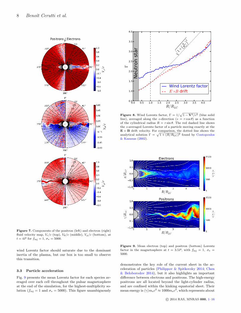
Fig. 7 shows the fluid velocity maps of each component,for both positrons (left panels) and electrons (right panels)in the inner magnetosphere at time t = 4P , where finj = 1and σ? = 5000. In the radial direction (top panel), both theelectrons and positrons fly outward along the open field linesalmost everywhere with a velocity of order Vr/c ≈ +0.8−0.9at r ≈ RLC and increasing with radius, with the notable ex-ceptions of the polar regions and in the current sheets. Thisradial motion is due to the Eθ × Bφ drift. At the poles,electrons and positrons both fly away from the star but atdifferent velocities. Electrons move at Vr/c ≈ +0.8 whilepositrons move at about Vr/c ≈ +0.1 only. Hence, in addi-tion to the net negative charge density at the poles, this dif-ference in velocity between the two species also contributesto the negative radial current shown in Fig. 3, middle panels.

In the current sheet, we discover that the two speciescounter-propagate with very high speeds: positrons areejected outward at +0.6c, while electrons precipitate backtowards the star at about −0.6c (appearing as a brightblue beam in Fig. 7, top right panel). As discussed below,this result has important consequences for particle acceler-ation and radiation. The Vθ-component does not show sig-nificant differences between electrons and positrons. Both

0 1 2 3 4 5r/RLC

0.0

0.2

0.4

0.6

0.8

1.0

1.2

L/L

0

Neut

ron

star

t/P=2.25

finj=0.1

finj=0.2

finj=0.5

finj=1

Figure 6. Outgoing Poynting flux integrated over a sphere of ra-

dius r, as function of radius at time t = 2.25P , for finj = 0.1 (blue

dotted line), 0.2 (green dashed-dotted line), 0.5 (red dashed line),and 1 (black solid line). The energy flux is normalized to the an-

alytic spin-down power of an aligned pulsar, L0 = cB2?r

6?/4R

4LC.

The disk-dome solution is not shown here because it does not spindown, L(r) = 0.

species have mildly relativistic (≈ 0.5c) drift velocities fromthe open field lines towards the current sheets, the highestspeeds being closest to the sheet. These converging flowsmaintain and feed the current sheets with fresh plasma.They do not appear in the split-monopole model (e.g.,Michel 1973), because they are caused by reconnection inthe equatorial layer which is captured by the simulations(see also Tchekhovskoy et al. 2013). The fluid velocity alongthe φ-direction highlights the fast rotation about the axis ofthe plasma in the current sheet.

By combining all these data together, we infer the bulkLorentz factor of the wind, Γ = 1/

√1− (V/c)2. Fig. 8

presents the variations of Γ as a function of the cylindricalradius (R = r sin θ), averaged along the z-direction (wherez = r cos θ). This figure also compares the Lorentz factorof the wind with the Lorentz factor of a particle moving atthe E × B drift velocity, Γdrift (red dashed line in Fig. 8).The wind starts with Γ ≈ 1.6 which depends on the initialvelocity of the injected particles. Then, Γ increases slowlywith distance until it coincides with the E×B drift Lorentzfactor at R ≈ 2.5RLC. At this point, the wind Lorentzfactor follows almost exactly the linear increase of Γdrift

with distance, in agreement with previous works (Buckley1977; Contopoulos & Kazanas 2002; Komissarov 2006; Buc-ciantini et al. 2006). We note that Γdrift follows perfectlythe Γdrift =

√1 + (R/RLC)2 solution found by Contopoulos

& Kazanas (2002) within the light cylinder (dotted line inFig. 8). Our solution deviates from this analytical expres-sion in the region 1 . R/RLC . 3, but it tends back tothe expected linear increase of Γ with R further out. At theouter edge of the box (R = 4.5RLC), the wind Lorentz factorreaches about Γ ≈ 3.5. In principle, the wind should accel-erate up to the fast magnetosonic point, beyond which the

c© 2014 RAS, MNRAS 000, 1–16

8 Benoıt Cerutti et al.

Figure 7. Components of the positron (left) and electron (right)fluid velocity map, Vr/c (top), Vθ/c (middle), Vφ/c (bottom), att = 4P for finj = 1, σ? = 5000.

wind Lorentz factor should saturate due to the dominantinertia of the plasma, but our box is too small to observethis transition.

3.3 Particle acceleration

Fig. 9 presents the mean Lorentz factor for each species av-eraged over each cell throughout the pulsar magnetosphereat the end of the simulation, for the highest-multiplicity so-lution (finj = 1 and σ? = 5000). This figure unambiguously

0.0 0.5 1.0 1.5 2.0 2.5 3.0 3.5 4.0R/RLC

0.5

1.0

1.5

2.0

2.5

3.0

3.5

4.0

Γ

√ 1+( R

R LC

) 2

Neut

ron

star

Wind Lorentz factorE×B drift

Figure 8. Wind Lorentz factor, Γ = 1/√

1−V2/c2 (blue solid

line), averaged along the z-direction (z = r cos θ) as a function

of the cylindrical radius R = r sin θ. The red dashed line showsthe z-averaged Lorentz factor of a particle moving exactly at the

E × B drift velocity. For comparison, the dotted line shows the

analytical solution Γ =√

1 + (R/RLC)2 found by Contopoulos& Kazanas (2002).

Figure 9. Mean electron (top) and positron (bottom) Lorentzfactor in the magnetosphere at t = 3.5P , with finj = 1, σ? =

5000.

demonstrates the key role of the current sheet in the ac-celeration of particles (Philippov & Spitkovsky 2014; Chen& Beloborodov 2014), but it also highlights an importantdifference between electrons and positrons. The high-energypositrons are all located beyond the light-cylinder radius,and are confined within the kinking equatorial sheet. Theirmean energy is 〈γ〉mec

2 ≈ 1000mec2, which represents about

c© 2014 RAS, MNRAS 000, 1–16

Particle acceleration in axisymmetric pulsar current sheets 9

100 101 102 103 104

γ

10-3

10-2

10-1

100

γ

Ntot

dN dγ

γ=σLC

Injection

Wind

Sheet

Particle energy spectra

ElectronsPositrons

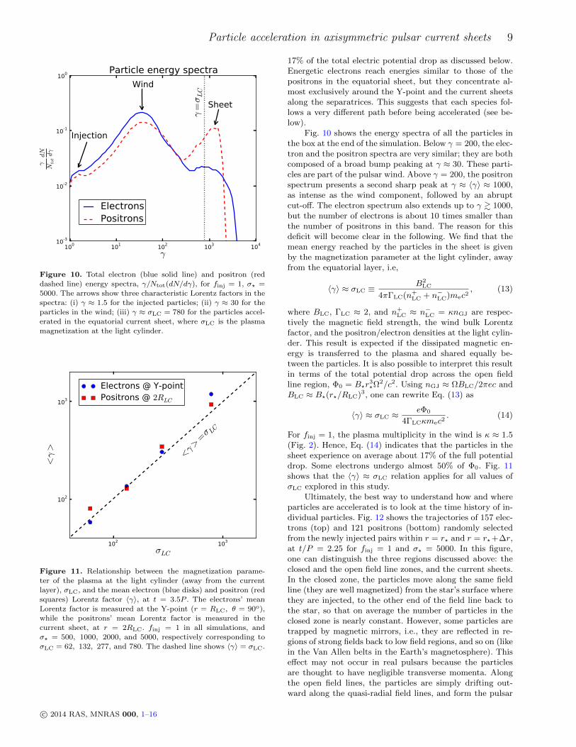
Figure 10. Total electron (blue solid line) and positron (red

dashed line) energy spectra, γ/Ntot(dN/dγ), for finj = 1, σ? =

5000. The arrows show three characteristic Lorentz factors in thespectra: (i) γ ≈ 1.5 for the injected particles; (ii) γ ≈ 30 for the

particles in the wind; (iii) γ ≈ σLC = 780 for the particles accel-

erated in the equatorial current sheet, where σLC is the plasmamagnetization at the light cylinder.

102 103

σLC

102

103

<γ>

<γ>

=σ LC

Electrons @ Y-pointPositrons @ 2RLC

Figure 11. Relationship between the magnetization parame-

ter of the plasma at the light cylinder (away from the currentlayer), σLC, and the mean electron (blue disks) and positron (redsquares) Lorentz factor 〈γ〉, at t = 3.5P . The electrons’ mean

Lorentz factor is measured at the Y-point (r = RLC, θ = 90o),while the positrons’ mean Lorentz factor is measured in the

current sheet, at r = 2RLC. finj = 1 in all simulations, and

σ? = 500, 1000, 2000, and 5000, respectively corresponding toσLC = 62, 132, 277, and 780. The dashed line shows 〈γ〉 = σLC.

17% of the total electric potential drop as discussed below.Energetic electrons reach energies similar to those of thepositrons in the equatorial sheet, but they concentrate al-most exclusively around the Y-point and the current sheetsalong the separatrices. This suggests that each species fol-lows a very different path before being accelerated (see be-low).

Fig. 10 shows the energy spectra of all the particles inthe box at the end of the simulation. Below γ = 200, the elec-tron and the positron spectra are very similar; they are bothcomposed of a broad bump peaking at γ ≈ 30. These parti-cles are part of the pulsar wind. Above γ = 200, the positronspectrum presents a second sharp peak at γ ≈ 〈γ〉 ≈ 1000,as intense as the wind component, followed by an abruptcut-off. The electron spectrum also extends up to γ & 1000,but the number of electrons is about 10 times smaller thanthe number of positrons in this band. The reason for thisdeficit will become clear in the following. We find that themean energy reached by the particles in the sheet is givenby the magnetization parameter at the light cylinder, awayfrom the equatorial layer, i.e,

〈γ〉 ≈ σLC ≡B2

LC

4πΓLC(n+LC + n−LC)mec2

, (13)

where BLC, ΓLC ≈ 2, and n+LC ≈ n−LC = κnGJ are respec-

tively the magnetic field strength, the wind bulk Lorentzfactor, and the positron/electron densities at the light cylin-der. This result is expected if the dissipated magnetic en-ergy is transferred to the plasma and shared equally be-tween the particles. It is also possible to interpret this resultin terms of the total potential drop across the open fieldline region, Φ0 = B?r

3?Ω

2/c2. Using nGJ ≈ ΩBLC/2πec andBLC ≈ B?(r?/RLC)3, one can rewrite Eq. (13) as

〈γ〉 ≈ σLC ≈eΦ0

4ΓLCκmec2. (14)

For finj = 1, the plasma multiplicity in the wind is κ ≈ 1.5(Fig. 2). Hence, Eq. (14) indicates that the particles in thesheet experience on average about 17% of the full potentialdrop. Some electrons undergo almost 50% of Φ0. Fig. 11shows that the 〈γ〉 ≈ σLC relation applies for all values ofσLC explored in this study.

Ultimately, the best way to understand how and whereparticles are accelerated is to look at the time history of in-dividual particles. Fig. 12 shows the trajectories of 157 elec-trons (top) and 121 positrons (bottom) randomly selectedfrom the newly injected pairs within r = r? and r = r?+∆r,at t/P = 2.25 for finj = 1 and σ? = 5000. In this figure,one can distinguish the three regions discussed above: theclosed and the open field line zones, and the current sheets.In the closed zone, the particles move along the same fieldline (they are well magnetized) from the star’s surface wherethey are injected, to the other end of the field line back tothe star, so that on average the number of particles in theclosed zone is nearly constant. However, some particles aretrapped by magnetic mirrors, i.e., they are reflected in re-gions of strong fields back to low field regions, and so on (likein the Van Allen belts in the Earth’s magnetosphere). Thiseffect may not occur in real pulsars because the particlesare thought to have negligible transverse momenta. Alongthe open field lines, the particles are simply drifting out-ward along the quasi-radial field lines, and form the pulsar

c© 2014 RAS, MNRAS 000, 1–16

10 Benoıt Cerutti et al.

0.0 0.5 1.0 1.5 2.0R/RLC

1.0

0.5

0.0

0.5

1.0

z/RLC

Star

Tracked electrons

0.0 0.5 1.0 1.5 2.0R/RLC

1.0

0.5

0.0

0.5

1.0

z/RLC

Star

Tracked positrons

Figure 12. Trajectories of a sample of 157 electrons (top) and

121 positrons (bottom) followed from the time of their injection att = 2.25P at the surface of the star, for about 2 rotation periods,

extracted from the run with finj = 1 and σ? = 5000. The vertical

dashed line indicates the light-cylinder radius. Magnetic fieldslines are omitted for clarity.

wind. At the poles, we note that some positrons are pushedback towards the star very soon after their injection (theseparticles are not shown here). This is due to the surface elec-tric field that sorts the particles to maintain a net negativecharge, and the required electric current, at the poles. Fi-nally, the current sheets are identified by the particles mov-ing along the boundary between the open and closed fieldline regions. Once these particles leave the separatrices, theyare trapped along the equatorial current sheet where theyfollow relativistic Speiser orbits (Speiser 1965; Contopoulos2007; Uzdensky et al. 2011; Cerutti et al. 2012).

We identify the regions of intense particle accelerationby selecting the particles according to their energy only.

0.0 0.5 1.0 1.5 2.0R/RLC

1.0

0.5

0.0

0.5

1.0

z/RLC

StarStarStarStarStar

Energetic particles (γ>1000)

Figure 13. Trajectories of all the particles (electrons in blue,

positrons in red) that reach a Lorentz factor γ > 1000 at leastonce in their history, from the sample shown in Fig. 12. The black

lines are magnetic field lines at the time when the particles were

injected, i.e., at t = 2.25P .

Fig. 13 shows the trajectories of all the energetic particlesfrom the sample (electrons in blue, positrons in red) whoseLorentz factor reach at least γ = 1000 during their his-tory. These high-energy electrons represent about 2% of theelectrons and about 40% of the total energy carried awayby the electrons (see Fig. 10). Energetic positrons repre-sent about 10% of all the positrons, carrying about 50% ofthe total positron energy. Drawn together, these orbits areexclusively confined to the current sheet regions (both theseparatrices and the equatorial sheets, as shown in Fig. 9).More specifically, all the high-energy particles originate froma narrow range of magnetic footpoints on the surface of thestar, spanning from about θ ∼ 42o-44o for the positrons, andθ ∼ 37o-40o for the electrons (note that these angles dependon the r?/RLC ratio).

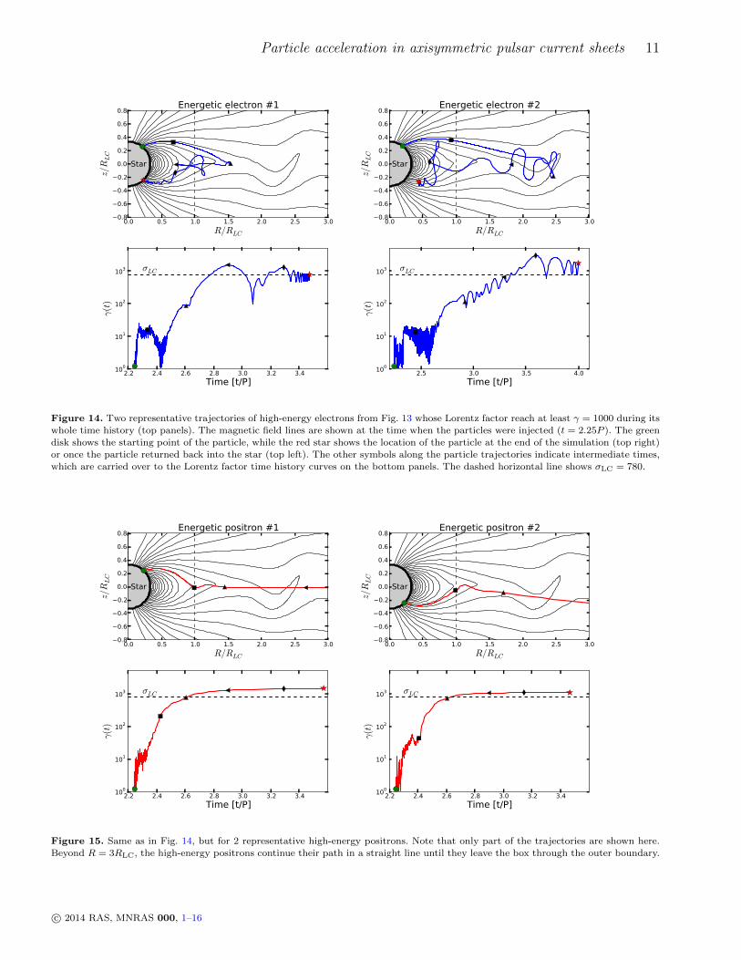
The particles get most of their energy once they reachthe equatorial current sheet. Figs. 14, 15 show representativetrajectories of energetic electrons and positrons taken fromthe sample, as well as the time evolution of their Lorentzfactors. For positrons, after a first energy gain from γ ≈ 1to γ & 10 close to the star, the bulk of the acceleration oc-curs at the Y-point over a distance of order the light-cylinderradius (see Fig. 15). Thereafter, their energy increases littlewith distance. In contrast, the high-energy electrons enterthe current sheet further away, typically at r & 1-2RLC andprecipitate back towards the star, counter-streaming againstthe outflowing positrons, in agreement with the two-fluidpicture drawn in the previous section (Fig. 7, top panel). Asthe electrons precipitate, their energy increases almost lin-early until they reach the Y-point. At this point, they bounceon the closed zone and flow back towards the star throughthe separatrices (see Fig. 14). The counter-streaming of elec-trons and positrons is maintained throughout the simulationby a non-zero radial electric field in the equatorial current

c© 2014 RAS, MNRAS 000, 1–16

Particle acceleration in axisymmetric pulsar current sheets 11

0.0 0.5 1.0 1.5 2.0 2.5 3.0R/RLC

0.8

0.6

0.4

0.2

0.0

0.2

0.4

0.6

0.8z/RLC

Star

Energetic electron #1

2.2 2.4 2.6 2.8 3.0 3.2 3.4Time [t/P]

100

101

102

103

γ(t

)

σLC

0.0 0.5 1.0 1.5 2.0 2.5 3.0R/RLC

0.8

0.6

0.4

0.2

0.0

0.2

0.4

0.6

0.8

z/RLC

Star

Energetic electron #2

2.5 3.0 3.5 4.0Time [t/P]

100

101

102

103

γ(t

)

σLC

Figure 14. Two representative trajectories of high-energy electrons from Fig. 13 whose Lorentz factor reach at least γ = 1000 during its

whole time history (top panels). The magnetic field lines are shown at the time when the particles were injected (t = 2.25P ). The greendisk shows the starting point of the particle, while the red star shows the location of the particle at the end of the simulation (top right)

or once the particle returned back into the star (top left). The other symbols along the particle trajectories indicate intermediate times,which are carried over to the Lorentz factor time history curves on the bottom panels. The dashed horizontal line shows σLC = 780.

0.0 0.5 1.0 1.5 2.0 2.5 3.0R/RLC

0.8

0.6

0.4

0.2

0.0

0.2

0.4

0.6

0.8

z/RLC

Star

Energetic positron #1

2.2 2.4 2.6 2.8 3.0 3.2 3.4Time [t/P]

100

101

102

103

γ(t

)

σLC

0.0 0.5 1.0 1.5 2.0 2.5 3.0R/RLC

0.8

0.6

0.4

0.2

0.0

0.2

0.4

0.6

0.8

z/RLC

Star

Energetic positron #2

2.2 2.4 2.6 2.8 3.0 3.2 3.4Time [t/P]

100

101

102

103

γ(t

)

σLC

Figure 15. Same as in Fig. 14, but for 2 representative high-energy positrons. Note that only part of the trajectories are shown here.Beyond R = 3RLC, the high-energy positrons continue their path in a straight line until they leave the box through the outer boundary.

c© 2014 RAS, MNRAS 000, 1–16

12 Benoıt Cerutti et al.

sheet (see also Contopoulos 2007). Electron orbits in thesheet also differ from positron orbits because the energeticelectrons are moving against the radial E×B drift while thepositrons are moving with it1. This difference is exaggeratedby the large amplitude of the electron orbits with respectto the layer mid-plane. Presumably, these excursions wouldrapidly disappear in real pulsars because the perpendicu-lar momentum of the particle would be efficiently radiatedaway. In addition, the thickness of the current sheet woulddecrease in reaction to the loss of pressure support in thepresence of radiative losses (Uzdensky & McKinney 2011;Cerutti et al. 2013). The effect of radiative colling on thepulsar magnetosphere will be explored elsewhere.

4 CONCLUSIONS

We have solved for the structure of the aligned pulsar mag-netosphere as a function of the plasma injection rate andmagnetization, using high-resolution 2D axisymmetric PICsimulations. Fresh electron-positron pairs are injected at aconstant rate with a non-zero velocity from the surface ofthe star to mimic pair production. If the plasma supply islow, the magnetosphere is highly charge-separated with elec-trons concentrated at the poles and positrons mostly in theequatorial regions. The pulsar luminosity is smaller than theexpected force-free spin-down power of an aligned rotator,and presents a high dissipation rate (& 40%) of the Poyntingflux beyond the light cylinder. This solution resembles themodel recently proposed by Contopoulos et al. (2014), inwhich there are no separatrices or Y-point and the currentlayer is electrostatically supported. In the extreme regimewhere there is no pair production, our solution collapses tothe static disk-dome solution of “dead” pulsars.

In contrast, we recover a nearly force-free solution ofthe magnetosphere in the high-multiplicity regime, with theexpected spin-down power of an aligned pulsar. A strongcurrent layer forms self-consistently beyond the light cylin-der and along the equator, which supports open, quasi-monopolar, magnetic field lines. We find that about 30%of the outgoing Poynting flux is dissipated in the currentlayer, mostly in the vicinity of the Y-point (Philippov &Spitkovsky 2014). These results imply that the pulsar mag-netosphere is highly sensitive to dissipation, consistent withearlier force-free simulations, having resistivity effectivelyconfined to the equatorial current sheet, in which more than20% of the spin-down power was dissipated within ten light-cylinder radii (Parfrey et al. 2012).

This dissipated energy is efficiently transferred to par-ticles in the current sheet. The simulations show that themean Lorentz factor of the energetic particles is given bythe upstream magnetization parameter at the light cylinder,i.e., 〈γ〉 ≈ σLC (Philippov & Spitkovsky 2014). We foundthat the high-energy particles follow one of two particulartrajectories in the magnetosphere. They all originate fromthe boundary layer between the closed and open magneticfield line regions, with a slight offset between electrons andpositrons. High-energy positrons stream outward along the

1 This effect was brought to our attention by the referee IoannisContopoulos.

separatrix with little change of energy until they reach theY-point. At this point, there are linearly accelerated in theequatorial sheet by the reconnection electric field, over a dis-tance of order the light-cylinder radius. Energetic electronsonly enter the layer further downstream and precipitate backtowards the star. Electrons are energized on their way to theY-point where their acceleration stops abruptly; they thenflow back onto the star along the separatrix. This mecha-nism naturally leads to an excess of energetic positrons flyingaway from the pulsar. In another publication, we will exploreif this result can be related to the contribution of pulsars tothe rising positron fraction measured by PAMELA (Adrianiet al. 2009).

Our results suggest that the current sheet, and the sep-aratrix layers, should be intense sources of high-energy ra-diation in pulsars (Lyubarskii 1996; Kirk et al. 2002; Bai &Spitkovsky 2010; Petri 2012a; Arka & Dubus 2013; Uzden-sky & Spitkovsky 2014). The precipitation of the energeticelectrons onto the star may be an additional source of radia-tion, an “auroral”-like emission (Arons 2012). The particlesin the wind (outside the layer) follow the E×B drift veloc-ity. These particles experience no radiative losses and littleradiation is expected from this region, unless they upscatterbackground radiation via inverse-Compton scattering (Ball& Kirk 2000; Bogovalov & Aharonian 2000; Cerutti et al.2008; Aharonian et al. 2012). Our simulations ignore syn-chrotron or curvature radiation cooling which should be im-portant in young pulsars, although we anticipate that theoverall structure of the magnetosphere and the accelerationmechanism reported here should be preserved. The otherimportant limitation of this work is the simplistic particleinjection. The next logical step towards the understandingof the high-energy emission in pulsars is to perform 3D PICsimulations of the oblique rotator, and to include the physicsof pair production in the magnetosphere (Philippov et al.2014).

ACKNOWLEDGMENTS

We thank J. Arons, A. Beloborodov, A. Chen, D. Capri-oli, L. Sironi, A. Tchekhovskoy, and D. A. Uzdensky fordiscussions, and the referee Ioannis Contopoulos for hisvaluable comments on the manuscript. BC acknowledgessupport from the Lyman Spitzer Jr. Fellowship awardedby the Department of Astrophysical Sciences at PrincetonUniversity. This work was partially suppored by the Max-Planck/Princeton Center for Plasma Physics, by NASAgrants NNX12AD01G and NNX13AO80G, and by the Si-mons Foundation (grant 291817 to AS). Computing re-sources were provided by the PICSciE-OIT TIGRESS HighPerformance Computing Center and Visualization Labora-tory at Princeton University.

REFERENCES

Abdo, A. A., Ajello, M., Allafort, A., et al. 2013, ApJS,208, 17

Adriani, O., Barbarino, G. C., Bazilevskaya, G. A., et al.2009, Nature, 458, 607

c© 2014 RAS, MNRAS 000, 1–16

Particle acceleration in axisymmetric pulsar current sheets 13

Aharonian, F. A., Bogovalov, S. V., & Khangulyan, D.2012, Nature, 482, 507

Arka, I. & Dubus, G. 2013, A&A, 550, A101Arons, J. 1983, ApJ, 266, 215Arons, J. 2012, Space Sci. Rev., 173, 341Bai, X.-N. & Spitkovsky, A. 2010, ApJ, 715, 1282Ball, L. & Kirk, J. G. 2000, Astroparticle Physics, 12, 335Belyaev, M. A. 2015, New Astronomy, 36, 37Birdsall, C. K. & Langdon, A. B. 1991, Plasma Physics viaComputer Simulation

Bogovalov, S. V. & Aharonian, F. A. 2000, MNRAS, 313,504

Bucciantini, N., Thompson, T. A., Arons, J., Quataert, E.,& Del Zanna, L. 2006, MNRAS, 368, 1717

Buckley, R. 1977, MNRAS, 180, 125Cerutti, B., Dubus, G., & Henri, G. 2008, A&A, 488, 37Cerutti, B., Uzdensky, D. A., & Begelman, M. C. 2012,ApJ, 746, 148

Cerutti, B., Werner, G. R., Uzdensky, D. A., & Begelman,M. C. 2013, ApJ, 770, 147

Cerutti, B., Werner, G. R., Uzdensky, D. A., & Begelman,M. C. 2014, ApJ, 782, 104

Chen, A. Y. & Beloborodov, A. M. 2014, ApJ, 795, L22Cheng, K. S., Ho, C., & Ruderman, M. 1986, ApJ, 300, 500Contopoulos, I. 2007, A&A, 472, 219Contopoulos, I., Kalapotharakos, C., & Kazanas, D. 2014,ApJ, 781, 46

Contopoulos, I. & Kazanas, D. 2002, ApJ, 566, 336Contopoulos, I., Kazanas, D., & Fendt, C. 1999, ApJ, 511,351

Coroniti, F. V. 1990, ApJ, 349, 538Goldreich, P. & Julian, W. H. 1969, ApJ, 157, 869Gruzinov, A. 2005, Physical Review Letters, 94, 021101Guo, F., Li, H., Daughton, W., & Liu, Y.-H. 2014, PhysicalReview Letters, 113, 155005

Jaroschek, C. H., Treumann, R. A., Lesch, H., & Scholer,M. 2004, Physics of Plasmas, 11, 1151

Kalapotharakos, C. & Contopoulos, I. 2009, A&A, 496, 495Kalapotharakos, C., Kazanas, D., Harding, A., & Con-topoulos, I. 2012, ApJ, 749, 2

Kirk, J. G., Skjæraasen, O., & Gallant, Y. A. 2002, A&A,388, L29

Komissarov, S. S. 2006, MNRAS, 367, 19Krause-Polstorff, J. & Michel, F. C. 1985, A&A, 144, 72Li, J., Spitkovsky, A., & Tchekhovskoy, A. 2012, ApJ, 746,60

Lyubarskii, Y. E. 1996, A&A, 311, 172McKinney, J. C. 2006, MNRAS, 368, L30Michel, F. C. 1973, ApJ, 180, L133Michel, F. C. & Li, H. 1999, Phys. Rep., 318, 227Muslimov, A. G. & Harding, A. K. 2003, ApJ, 588, 430Parfrey, K., Beloborodov, A. M., & Hui, L. 2012, MNRAS,423, 1416

Petri, J. 2012a, MNRAS, 424, 2023Petri, J. 2012b, MNRAS, 424, 605Petri, J., Heyvaerts, J., & Bonazzola, S. 2002, A&A, 384,414

Philippov, A. A. & Spitkovsky, A. 2014, ApJ, 785, L33Philippov, A. A., Spitkovsky, A., & Cerutti, B. 2014, ArXive-prints

Pritchett, P. L. 2003, in Lecture Notes in Physics, BerlinSpringer Verlag, Vol. 615, Space Plasma Simulation, ed.

J. Buchner, C. Dum, & M. Scholer, 1–24Romani, R. W. 1996, ApJ, 470, 469Sironi, L. & Spitkovsky, A. 2014, ApJ, 783, L21Smith, I. A., Michel, F. C., & Thacker, P. D. 2001, MNRAS,322, 209

Speiser, T. W. 1965, J. Geophys. Res., 70, 4219Spitkovsky, A. 2006, ApJ, 648, L51Spitkovsky, A. & Arons, J. 2002, in Astronomical Societyof the Pacific Conference Series, Vol. 271, Neutron Stars inSupernova Remnants, ed. P. O. Slane & B. M. Gaensler,81

Tchekhovskoy, A., Spitkovsky, A., & Li, J. G. 2013, MN-RAS, 435, L1

Timokhin, A. N. 2006, MNRAS, 368, 1055Timokhin, A. N. & Arons, J. 2013, MNRAS, 429, 20Uzdensky, D. A., Cerutti, B., & Begelman, M. C. 2011,ApJ, 737, L40

Uzdensky, D. A. & McKinney, J. C. 2011, Physics of Plas-mas, 18, 042105

Uzdensky, D. A. & Spitkovsky, A. 2014, ApJ, 780, 3Vay, J.-L. 2008, Physics of Plasmas, 15, 056701Werner, G. R., Uzdensky, D. A., Cerutti, B., Nalewajko,K., & Begelman, M. C. 2014, ArXiv e-prints

Yee, K. 1966, IEEE Transactions on Antennas and Propa-gation, 14, 302

Zenitani, S. & Hoshino, M. 2001, ApJ, 562, L63

c© 2014 RAS, MNRAS 000, 1–16

14 Benoıt Cerutti et al.

(i, j+ 12 )

(i, j)

(i+ 12 , j)

Eφ,Jφ

Bφ

Er,Jr

Eθ,Jθ

Br

Bθ

Figure A1. Two-dimensional spherical Yee-lattice adopted in Zeltron.

APPENDIX A: INTEGRATION OF MAXWELL’S EQUATIONS ON THE 2D SPHERICAL YEE GRID

In this appendix, we derive the expressions of the differential operators ∇ × E, ∇ ×B, ∇ · E and ∇2 integrated over a 2Daxisymmetric cell defined in spherical coordinates (so that any derivative in the azimuthal direction vanishes, ∂/∂φ = 0), asimplemented in Zeltron to solve Maxwell’s equations. Each cell is labeled by the integers (i,j), i for the radial direction, andj for the θ-direction. The fields are defined on the Yee lattice which is staggered by half a grid cell in both spatial directions,as shown in Fig. A1.∇×E and ∇×B can easily be integrated using Stokes’ theorem on one cell, i.e.,

¨S

(∇×E) · dS =

˛C

E · dC, (A1)

where S is the surface vector pointing away from the cell, and C is the contour vector circulating around the cell. ApplyingEq. (A1) in each direction gives

(∇×E)ri,j+ 1

2

=sin θj+1Eφi,j+1 − sin θjEφi,j

ri∆µj+ 12

(A2)

(∇×E)θi+ 1

2,j

= −2(ri+1Eφi+1,j − riEφi,j

)∆r2

i+ 12

(A3)

(∇×E)φi+ 1

2,j+ 1

2

= −2∆ri+ 1

2

(Er

i+ 12,j+1− Er

i+12,j

)∆r2

i+ 12

∆θ+

2

(ri+1Eθ

i+1,j+ 12

− riEθi,j+ 1

2

)∆r2

i+ 12

, (A4)

where ∆µj+ 12

= (cos θj − cos θj+1), ∆ri+ 12

= (ri+1 − ri) and ∆r2i+ 1

2=(r2i+1 − r2i

). Similarly, integrating ∇ × B on the Yee

lattice yields

(∇×B)ri+ 1

2,j

=sin θj+ 1

2Bφ

i+ 12,j+ 1

2

− sin θj− 12Bφ

i+ 12,j− 1

2

ri+ 12∆µj

(A5)

(∇×B)θi,j+ 1

2

= −2

(ri+ 1

2Bφ

i+ 12,j+ 1

2

− ri− 12Bφ

i− 12,j+ 1

2

)∆r2i

(A6)

(∇×B)φi,j= −

2∆ri

(Br

i,j+ 12

−Bri,j− 1

2

)∆r2i ∆θ

+

2

(ri+ 1

2Bθ

i+ 12,j− ri− 1

2Bθ

i− 12,j

)∆r2i

, (A7)

with ∆µj =(

cos θj− 12− cos θj+ 1

2

), ∆ri =

(ri+ 1

2− ri− 1

2

)and ∆r2i =

(r2i+ 1

2− r2

i− 12

).

To integrate ∇ ·E, we make use of Gauss’ theorem˚V

(∇ · E) dV =

‹S

E · dS (A8)

c© 2014 RAS, MNRAS 000, 1–16

Particle acceleration in axisymmetric pulsar current sheets 15

(i,j+1)

(i,j)

(i+1,j)

(i+1,j+1)

θ

θj

θj+1

r

Vi,j

Vi+1,j

Vi+1,j+1Vi,j+1

φ = 0, 2π

Axis

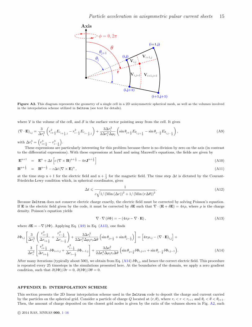
Figure A2. This diagram represents the geometry of a single cell in a 2D axisymmetric spherical mesh, as well as the volumes involvedin the interpolation scheme utilized in Zeltron (see text for details).

where V is the volume of the cell, and S is the surface vector pointing away from the cell. It gives

(∇ ·E)i,j =3

∆r3i

(r2i+ 1

2Er

i+ 12,j− r2i− 1

2Er

i− 12,j

)+

3∆r2i2∆r3i ∆µj

(sin θj+ 1

2Eθ

i,j+ 12

− sin θj− 12Eθ

i,j− 12

), (A9)

with ∆r3i =(r3i+ 1

2− r3

i− 12

).

These expressions are particularly interesting for this problem because there is no division by zero on the axis (in contrastto the differential expressions). With these expressions at hand and using Maxwell’s equations, the fields are given by

En+1 = En + ∆t[c (∇×B)n+

12 − 4πJn+ 1

2

](A10)

Bn+ 12 = Bn− 1

2 − c∆t (∇×E)n , (A11)

at the time step n + 1 for the electric field and n + 12

for the magnetic field. The time step ∆t is dictated by the Courant-Friedrichs-Lewy condition which, in spherical coordinates, gives

∆t 61

c√

1/ (Min (∆r))2 + 1/ (Min (r∆θ))2. (A12)

Because Zeltron does not conserve electric charge exactly, the electric field must be corrected by solving Poisson’s equation.If E is the electric field given by the code, it must be corrected by δE such that ∇ · (E + δE) = 4πρ, where ρ is the chargedensity. Poisson’s equation yields

∇ · ∇ (δΦ) = − (4πρ−∇ ·E) , (A13)

where δE = −∇ (δΦ). Applying Eq. (A9) in Eq. (A13), one finds

δΦi,j

[3

∆r3i

(r2i+ 1

2

∆ri+ 12

+r2i− 1

2

∆ri− 12

)+

3∆r2i2∆r3i ∆µjri∆θ

(sin θj+ 1

2+ sin θj− 1

2

)]=[4πρi,j − (∇ ·E)i,j

]+

3

∆r3i

[r2i+ 1

2

∆ri+ 12

δΦi+1,j +r2i− 1

2

∆ri− 12

δΦi−1,j

]+

3∆r2i2∆r3i ∆µjri∆θ

(sin θj+ 1

2δΦi,j+1 + sin θj− 1

2δΦi,j−1

). (A14)

After many iterations (typically about 500), we obtain from Eq. (A14) δΦi,j, and hence the correct electric field. This procedureis repeated every 25 timesteps in the simulations presented here. At the boundaries of the domain, we apply a zero gradientcondition, such that ∂(δΦ)/∂r = 0, ∂(δΦ)/∂θ = 0.

APPENDIX B: INTERPOLATION SCHEME

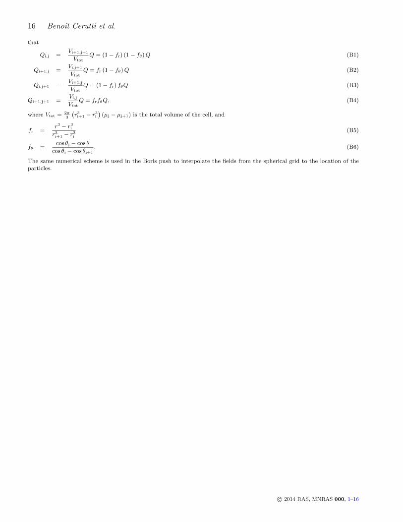
This section presents the 2D linear interpolation scheme used in the Zeltron code to deposit the charge and current carriedby the particles on the spherical grid. Consider a particle of charge Q located at (r, θ), where ri < r < ri+1 and θj < θ < θj+1.Then, the amount of charge deposited on the closest grid nodes is given by the ratio of the volumes shown in Fig. A2, such

c© 2014 RAS, MNRAS 000, 1–16

16 Benoıt Cerutti et al.

that

Qi,j =Vi+1,j+1

VtotQ = (1− fr) (1− fθ)Q (B1)

Qi+1,j =Vi,j+1

VtotQ = fr (1− fθ)Q (B2)

Qi,j+1 =Vi+1,j

VtotQ = (1− fr) fθQ (B3)

Qi+1,j+1 =Vi,j

VtotQ = frfθQ, (B4)

where Vtot = 2π3

(r3i+1 − r3i

)(µj − µj+1) is the total volume of the cell, and

fr =r3 − r3ir3i+1 − r3i

(B5)

fθ =cos θj − cos θ

cos θj − cos θj+1. (B6)

The same numerical scheme is used in the Boris push to interpolate the fields from the spherical grid to the location of theparticles.

c© 2014 RAS, MNRAS 000, 1–16