Partial Fraction Decomposition - unibo.itfioresi/2018/gen/lec5.pdf · Partial Fraction...

Section 7.4 Partial Fractions 531

Partial Fraction Decomposition

Algebraic techniques for determining the constants in the numerators of partial

fractions are demonstrated in the examples that follow. Note that the techniques vary

slightly, depending on the type of factors of the denominator: linear or quadratic,

distinct or repeated.

Distinct Linear Factors

Write the partial fraction decomposition of

Solution

The expression is proper, so be sure to factor the denominator. Because

you should include one partial fraction with a constant

numerator for each linear factor of the denominator. Write the form of the decomposition

as follows.

Write form of decomposition.

Multiplying each side of this equation by the least common denominator,

leads to the basic equation

Basic equation

Because this equation is true for all you can substitute any convenient values of that

will help determine the constants and Values of that are especially convenient are

ones that make the factors and equal to zero. For instance, let

Then

Substitute for

To solve for let and obtain

Substitute 3 for

So, the partial fraction decomposition is

Check this result by combining the two partial fractions on the right side of the

equation, or by using your graphing utility.

Now try Exercise 23.

x � 7

x2 � x � 6�

2

x � 3��1

x � 2.

2 � A.

10 � 5A

10 � A�5� � B�0�

x.3 � 7 � A�3 � 2� � B�3 � 3�

x � 3A,

�1 � B.

5 � �5B

5 � A�0� � B��5�

x.�2�2 � 7 � A��2 � 2� � B��2 � 3�

x � �2.�x � 3��x � 2�xB.A

xx,

x � 7 � A�x � 2� � B�x � 3�.

�x � 3��x � 2�,

x � 7

x2 � x � 6�

A

x � 3�

B

x � 2

x2 � x � 6 � �x � 3��x � 2�,

x � 7

x2 � x � 6.

Example 1

TECHNOLOGY

You can use a graphing utility tocheck the decomposition foundin Example 1. To do this, graph

and

in the same viewing window. Thegraphs should be identical, asshown below.

9−9

−6

6

y2 2

x ! 3"!1

x " 2

y1 x " 7

x2 ! x ! 6

532 Chapter 7 Systems of Equations and Inequalities

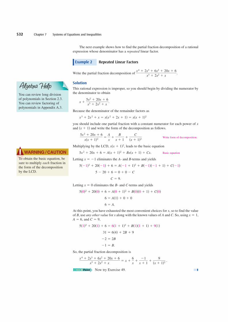
The next example shows how to find the partial fraction decomposition of a rational

expression whose denominator has a repeated linear factor.

Repeated Linear Factors


Solution

This rational expression is improper, so you should begin by dividing the numerator by

the denominator to obtain

Because the denominator of the remainder factors as

you should include one partial fraction with a constant numerator for each power of

and and write the form of the decomposition as follows.


Multiplying by the LCD, leads to the basic equation

Basic equation

Letting eliminates the - and -terms and yields

Letting eliminates the - and -terms and yields

At this point, you have exhausted the most convenient choices for so to find the value

of use any other value for along with the known values of and So, using

and



x �6

x��1

x � 1�

9

�x � 1�2 .

x4 � 2x3 � 6x2 � 20x � 6

x3 � 2x2 � x�

�1 � B.

�2 � 2B

31 � 6�4� � 2B � 9

5�1�2 � 20�1� � 6 � 6�1 � 1�2 � B�1��1 � 1� � 9�1�

C � 9,A � 6,

x � 1,C.AxB,

x,

6 � A.

6 � A�1� � 0 � 0

5�0�2 � 20�0� � 6 � A�0 � 1�2 � B�0��0 � 1� � C�0�

CBx � 0

C � 9.

5 � 20 � 6 � 0 � 0 � C

5��1�2 � 20��1� � 6 � A��1 � 1�2 � B��1��1 � 1� � C��1�

BAx � �1

5x2 � 20x � 6 � A�x � 1�2 � Bx�x � 1� � Cx.

x�x � 1�2,

5x2 � 20x � 6

x�x � 1�2�

A

x�

B

x � 1�

C

�x � 1�2

�x � 1�x

x3 � 2x2 � x � x�x2 � 2x � 1� � x�x � 1�2

x �5x2 � 20x � 6

x3 � 2x2 � x.

x4 � 2x3 � 6x2 � 20x � 6

x3 � 2x2 � x.

Example 2

You can review long division

of polynomials in Section 2.3.

You can review factoring of

polynomials in Appendix A.3.

WARNING / CAUTION

To obtain the basic equation, be

sure to multiply each fraction in

the form of the decomposition

by the LCD.


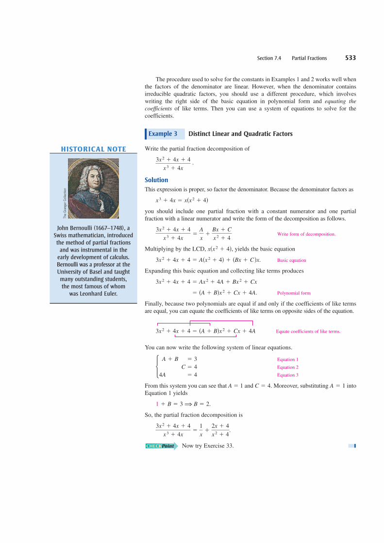
The procedure used to solve for the constants in Examples 1 and 2 works well when

the factors of the denominator are linear. However, when the denominator contains

irreducible quadratic factors, you should use a different procedure, which involves

writing the right side of the basic equation in polynomial form and equating the

coefficients of like terms. Then you can use a system of equations to solve for the

coefficients.

Distinct Linear and Quadratic Factors


Solution

This expression is proper, so factor the denominator. Because the denominator factors as

you should include one partial fraction with a constant numerator and one partial

fraction with a linear numerator and write the form of the decomposition as follows.


Multiplying by the LCD, yields the basic equation

Basic equation

Expanding this basic equation and collecting like terms produces

Polynomial form

Finally, because two polynomials are equal if and only if the coefficients of like terms

are equal, you can equate the coefficients of like terms on opposite sides of the equation.

Equate coefficients of like terms.

You can now write the following system of linear equations.

From this system you can see that and Moreover, substituting into

Equation 1 yields



3x2 � 4x � 4

x3 � 4x�1

x�2x � 4

x2 � 4.

1 � B � 3⇒ B � 2.

A � 1C � 4.A � 1

Equation 1

Equation 2

Equation 3�

A

4A

� B

C

�

�

�

3

4

4

3x2 � 4x � 4 � �A � B�x2 � Cx � 4A

� �A � B�x2 � Cx � 4A.

3x2 � 4x � 4 � Ax2 � 4A � Bx2 � Cx

3x2 � 4x � 4 � A�x2 � 4� � �Bx � C�x.

x�x2 � 4�,

3x2 � 4x � 4

x3 � 4x�

A

x�

Bx � C

x2 � 4

x3 � 4x � x�x2 � 4�

3x2 � 4x � 4

x3 � 4x.

Example 3

HISTORICAL NOTE

John Bernoulli (1667–1748), aSwiss mathematician, introducedthe method of partial fractions

and was instrumental in theearly development of calculus.Bernoulli was a professor at theUniversity of Basel and taughtmany outstanding students, the most famous of whom

was Leonhard Euler.

The Granger Collection

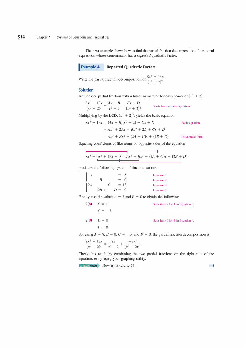
The next example shows how to find the partial fraction decomposition of a rational

expression whose denominator has a repeated quadratic factor.

Repeated Quadratic Factors


Solution

Include one partial fraction with a linear numerator for each power of


Multiplying by the LCD, yields the basic equation

Basic equation

Polynomial form

Equating coefficients of like terms on opposite sides of the equation

produces the following system of linear equations.

Finally, use the values and to obtain the following.

Substitute 8 for A in Equation 3.

Substitute 0 for B in Equation 4.

So, using and the partial fraction decomposition is

Check this result by combining the two partial fractions on the right side of the

equation, or by using your graphing utility.


8x3 � 13x

�x2 � 2�2�

8x

x2 � 2�

�3x

�x2 � 2�2.

D � 0,C � �3,B � 0,A � 8,

D � 0

2�0� � D � 0

C � �3

2�8� � C � 13

B � 0A � 8

Equation 1

Equation 2

Equation 3

Equation 4�

A

2A �

B

2B �

C

D

�

�

�

�

8

0

13

0

8x3 � 0x2 � 13x � 0 � Ax3 � Bx2 � �2A � C�x � �2B � D�

� Ax3 � Bx2 � �2A � C�x � �2B � D�.

� Ax3 � 2Ax � Bx2 � 2B � Cx � D

8x3 � 13x � �Ax � B��x2 � 2� � Cx � D

�x2 � 2�2,

8x3 � 13x

�x2 � 2�2�

Ax � B

x2 � 2�

Cx � D

�x2 � 2�2

�x2 � 2�.

8x3 � 13x

�x2 � 2�2.

Example 4



Keep in mind that for improper rational expressions such as

you must first divide before applying partial fraction decomposition.

N�x�D�x�

�2x3 � x2 � 7x � 7

x2 � x � 2

Guidelines for Solving the Basic Equation

Linear Factors

1. Substitute the zeros of the distinct linear factors into the basic equation.

2. For repeated linear factors, use the coefficients determined in Step 1 to rewrite

the basic equation. Then substitute other convenient values of and solve for

the remaining coefficients.

Quadratic Factors

1. Expand the basic equation.

2. Collect terms according to powers of

3. Equate the coefficients of like terms to obtain equations involving

and so on.

4. Use a system of linear equations to solve for A, B, C, . . . .

C,A, B,

x.

x

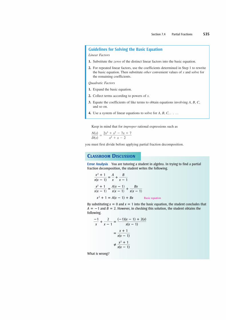
Error Analysis You are tutoring a student in algebra. In trying to find a partial fraction decomposition, the student writes the following.

Basic equation

By substituting and into the basic equation, the student concludes thatand However, in checking this solution, the student obtains the

following.

What is wrong?

#x2 " 1

x x ! 1!

x " 1

x x ! 1!

!1

x"

2

x ! 1

!1! x ! 1! " 2 x!x x ! 1!

B 2.A !1x 1x 0

x2 " 1 A x ! 1! " Bx

x2 " 1

x�x ! 1�

A�x ! 1�x�x ! 1�

"Bx

x�x ! 1�

x2 " 1

x x ! 1!

A

x"

B

x ! 1

CLASSROOM DISCUSSION


EXERCISES See www.CalcChat.com for worked-out solutions to odd-numbered exercises.7.4

VOCABULARY: Fill in the blanks.

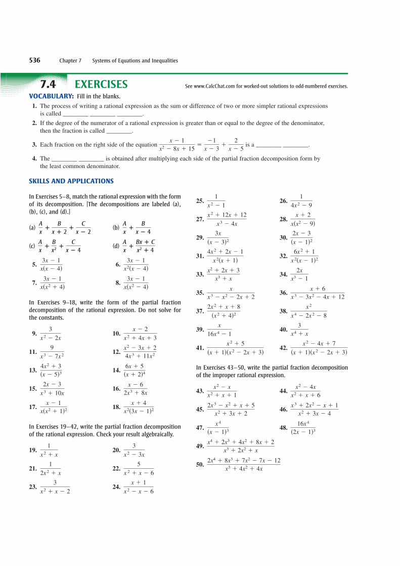
1. The process of writing a rational expression as the sum or difference of two or more simpler rational expressions

is called ________ ________ ________.

2. If the degree of the numerator of a rational expression is greater than or equal to the degree of the denominator,

then the fraction is called ________.

3. Each fraction on the right side of the equation is a ________ ________.

4. The ________ ________ is obtained after multiplying each side of the partial fraction decomposition form by

the least common denominator.

SKILLS AND APPLICATIONS

x � 1

x2 � 8x � 15��1

x � 3�

2

x � 5

In Exercises 5–8, match the rational expression with the formof its decomposition. [The decompositions are labeled (a),(b), (c), and (d).]

(a) (b)

(c) (d)

5. 6.

7. 8.

In Exercises 9–18, write the form of the partial fractiondecomposition of the rational expression. Do not solve forthe constants.

9. 10.

11. 12.

13. 14.

15. 16.

17. 18.

In Exercises 19–42, write the partial fraction decompositionof the rational expression. Check your result algebraically.

19. 20.

21. 22.

23. 24.

25. 26.

27. 28.

29. 30.

31. 32.

33. 34.

35. 36.

37. 38.

39. 40.

41. 42.

In Exercises 43–50, write the partial fraction decompositionof the improper rational expression.

43. 44.

45. 46.

47. 48.

49.

50.2x4 � 8x3 � 7x2 � 7x � 12

x3 � 4x2 � 4x

x4 � 2x3 � 4x2 � 8x � 2

x3 � 2x2 � x

16x4

�2x � 1�3x4

�x � 1�3

x3 � 2x2 � x � 1

x2 � 3x � 4

2x3 � x2 � x � 5

x2 � 3x � 2

x2 � 4x

x2 � x � 6

x2 � x

x2 � x � 1

x2 � 4x � 7

�x � 1��x2 � 2x � 3�x2 � 5

�x � 1��x2 � 2x � 3�

3

x4 � x

x

16x4 � 1

x2

x4 � 2x2 � 8

2x2 � x � 8

�x2 � 4�2

x � 6

x3 � 3x2 � 4x � 12

x

x3 � x2 � 2x � 2

2x

x3 � 1

x2 � 2x � 3

x3 � x

6x2 � 1

x2�x � 1�24x2 � 2x � 1

x2�x � 1�

2x � 3

�x � 1�23x

�x � 3�2

x � 2

x�x2 � 9�x2 � 12x � 12

x3 � 4x

1

4x2 � 9

1

x2 � 1

x � 1

x2 � x � 6

3

x2 � x � 2

5

x 2 � x � 6

1

2x2 � x

3

x2 � 3x

1

x2 � x

x � 4

x2�3x � 1�2x � 1

x�x2 � 1�2

x � 6

2x3 � 8x

2x � 3

x3 � 10x

6x � 5

�x � 2�44x2 � 3

�x � 5�3

x2 � 3x � 2

4x3 � 11x29

x3 � 7x2

x � 2

x2 � 4x � 3

3

x2 � 2x

3x � 1

x�x2 � 4�3x � 1

x�x2 � 4�

3x � 1

x2�x � 4�3x � 1

x�x � 4�

A

x"

Bx " C

x2 " 4

A

x"

B

x2"

C

x ! 4

A

x"

B

x ! 4

A

x"

B

x " 2"

C

x ! 2


In Exercises 51–58, write the partial fraction decomposition ofthe rational expression. Use a graphing utility to check yourresult.

51. 52.

53. 54.

55. 56.

57. 58.

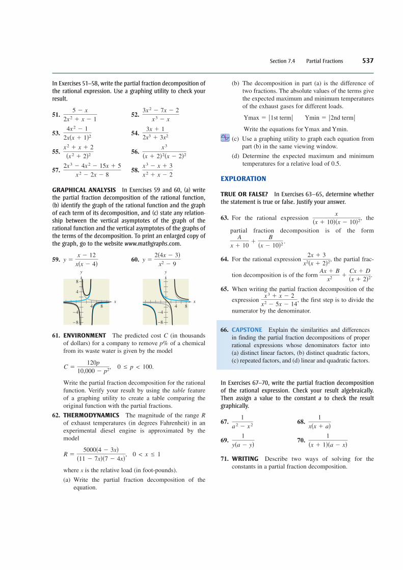
GRAPHICAL ANALYSIS In Exercises 59 and 60, (a) writethe partial fraction decomposition of the rational function,(b) identify the graph of the rational function and the graphof each term of its decomposition, and (c) state any relation-ship between the vertical asymptotes of the graph of therational function and the vertical asymptotes of the graphs ofthe terms of the decomposition. To print an enlarged copy ofthe graph, go to the website www.mathgraphs.com.

59. 60.

61. ENVIRONMENT The predicted cost (in thousands

of dollars) for a company to remove of a chemical

from its waste water is given by the model

Write the partial fraction decomposition for the rational

function. Verify your result by using the table feature

of a graphing utility to create a table comparing the

original function with the partial fractions.

62. THERMODYNAMICS The magnitude of the range

of exhaust temperatures (in degrees Fahrenheit) in an

experimental diesel engine is approximated by the

model

where is the relative load (in foot-pounds).

(a) Write the partial fraction decomposition of the

equation.

(b) The decomposition in part (a) is the difference of

two fractions. The absolute values of the terms give

the expected maximum and minimum temperatures

of the exhaust gases for different loads.

Write the equations for Ymax and Ymin.

(c) Use a graphing utility to graph each equation from

part (b) in the same viewing window.

(d) Determine the expected maximum and minimum

temperatures for a relative load of 0.5.

EXPLORATION

TRUE OR FALSE? In Exercises 63–65, determine whetherthe statement is true or false. Justify your answer.

63. For the rational expression the

partial fraction decomposition is of the form

64. For the rational expression the partial frac-

tion decomposition is of the form

65. When writing the partial fraction decomposition of the

expression the first step is to divide the

numerator by the denominator.

In Exercises 67–70, write the partial fraction decompositionof the rational expression. Check your result algebraically.Then assign a value to the constant to check the resultgraphically.

67. 68.

69. 70.

71. WRITING Describe two ways of solving for the

constants in a partial fraction decomposition.

1

�x � 1��a � x�1

y�a � y�

1

x�x � a�1

a2 � x2

a

x3 � x � 2

x2 � 5x � 14,

Ax � B

x2�

Cx � D

�x � 2�2.

2x � 3

x2�x � 2�2,

A

x � 10�

B

�x � 10�2.

x

�x � 10��x � 10�2,

Ymin � 2nd termYmax � 1st term

x

0 < x 1R �5000�4 � 3x�

�11 � 7x��7 � 4x�,

R

C �120p

10,000 � p2, 0 p < 100.

p%

C

4 8x

y

−4

−8

4 8

−8

−4

4

8

x

y

y �2�4x � 3�x2� 9

y �x � 12

x�x � 4�

x3� x � 3

x2� x � 2

2x3� 4x2

� 15x � 5

x2� 2x � 8

x3

�x � 2�2�x � 2�2

x2� x � 2

�x2� 2�2

3x � 1

2x3� 3x2

4x2� 1

2x�x � 1�2

3x2� 7x � 2

x3� x

5 � x

2x2� x � 1

66. CAPSTONE Explain the similarities and differences

in finding the partial fraction decompositions of proper

rational expressions whose denominators factor into

(a) distinct linear factors, (b) distinct quadratic factors,

(c) repeated factors, and (d) linear and quadratic factors.


7.5 SYSTEMS OF INEQUALITIES

What you should learn

• Sketch the graphs of inequalities in two variables.

• Solve systems of inequalities.

• Use systems of inequalities in twovariables to model and solve real-lifeproblems.

Why you should learn it

You can use systems of inequalities in two variables to model and solvereal-life problems. For instance, inExercise 83 on page 547, you will usea system of inequalities to analyze the retail sales of prescription drugs.

Jon Feingersh/Masterfile

The Graph of an Inequality

The statements and are inequalities in two variables. An

ordered pair is a solution of an inequality in and if the inequality is true when

and are substituted for and respectively. The graph of an inequality is the

collection of all solutions of the inequality. To sketch the graph of an inequality, begin

by sketching the graph of the corresponding equation. The graph of the equation will

normally separate the plane into two or more regions. In each such region, one of the

following must be true.

1. All points in the region are solutions of the inequality.

2. No point in the region is a solution of the inequality.

So, you can determine whether the points in an entire region satisfy the inequality by

simply testing one point in the region.

Sketching the Graph of an Inequality

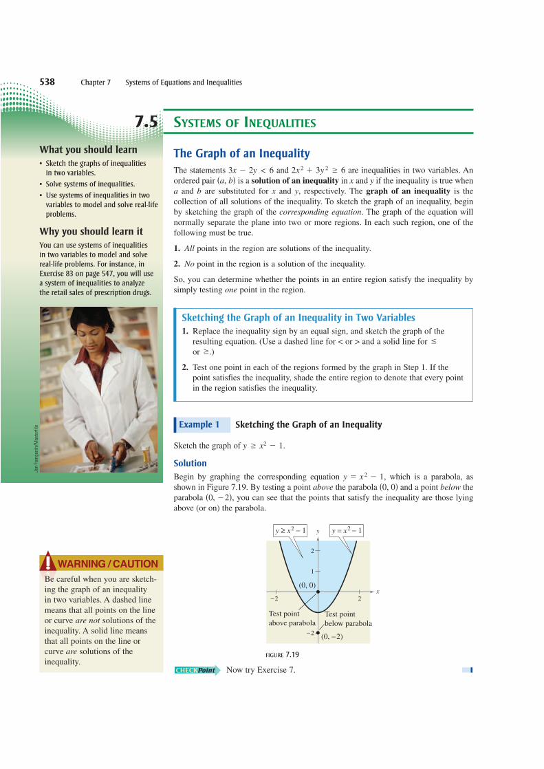
Sketch the graph of

Solution

Begin by graphing the corresponding equation which is a parabola, as

shown in Figure 7.19. By testing a point above the parabola and a point below the

parabola you can see that the points that satisfy the inequality are those lying

above (or on) the parabola.

FIGURE 7.19

Now try Exercise 7.

−2 2

−2

1

2

(0, 0)

(0, −2)

Test point

below parabola

Test point

above parabola

y = x2 − 1y ≥ x2 − 1 y

x

�0, �2�,�0, 0�

y � x2� 1,

y � x2� 1.

Example 1

y,xba

yx�a, b�2x2

� 3y 2� 63x � 2y < 6

WARNING / CAUTION

Be careful when you are sketch-

ing the graph of an inequality

in two variables. A dashed line

means that all points on the line

or curve are not solutions of the

inequality. A solid line means

that all points on the line or

curve are solutions of the

inequality.

Sketching the Graph of an Inequality in Two Variables

1. Replace the inequality sign by an equal sign, and sketch the graph of the

resulting equation. (Use a dashed line for < or > and a solid line for

or .)

2. Test one point in each of the regions formed by the graph in Step 1. If the

point satisfies the inequality, shade the entire region to denote that every point

in the region satisfies the inequality.

�

Section 7.5 Systems of Inequalities 539

The inequality in Example 1 is a nonlinear inequality in two variables. Most of the

following examples involve linear inequalities such as ( and are not

both zero). The graph of a linear inequality is a half-plane lying on one side of the line

Sketching the Graph of a Linear Inequality

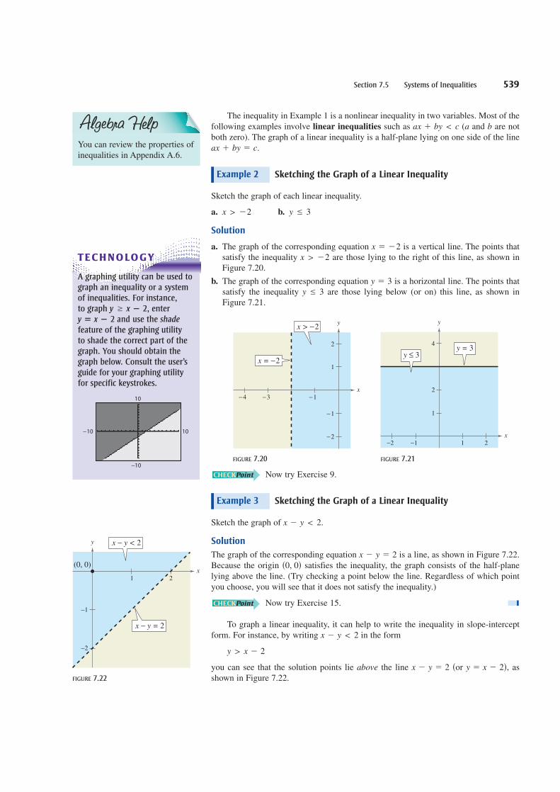
Sketch the graph of each linear inequality.

a. b.

Solution

a. The graph of the corresponding equation is a vertical line. The points that

satisfy the inequality are those lying to the right of this line, as shown in

Figure 7.20.

b. The graph of the corresponding equation is a horizontal line. The points that

satisfy the inequality are those lying below (or on) this line, as shown in

Figure 7.21.

FIGURE 7.20 FIGURE 7.21

Now try Exercise 9.

Sketching the Graph of a Linear Inequality

Sketch the graph of

Solution

The graph of the corresponding equation is a line, as shown in Figure 7.22.

Because the origin satisfies the inequality, the graph consists of the half-plane

lying above the line. (Try checking a point below the line. Regardless of which point

you choose, you will see that it does not satisfy the inequality.)


To graph a linear inequality, it can help to write the inequality in slope-intercept

form. For instance, by writing in the form

you can see that the solution points lie above the line or as

shown in Figure 7.22.

y � x � 2�,�x � y � 2

y > x � 2

x � y < 2

�0, 0�x � y � 2

x � y < 2.

Example 3

1

4

2

−2 −1 1 2

y ≤ 3

y

x

y = 3

−2

−1

1

2

−1−3−4

x > −2

x = −2

y

x

y 3

y � 3

x > �2

x � �2

y 3x > �2

Example 2

ax � by � c.

baax � by < c

TECHNOLOGY

A graphing utility can be used tograph an inequality or a systemof inequalities. For instance, to graph enter

and use the shadefeature of the graphing utility to shade the correct part of thegraph. You should obtain thegraph below. Consult the user’sguide for your graphing utilityfor specific keystrokes.

−10 10

−10

10

y x ! 2y � x ! 2,

−1

−2

x − y < 2

x − y = 2

1 2

(0, 0)

y

x

FIGURE 7.22

You can review the properties of

inequalities in Appendix A.6.

Systems of Inequalities

Many practical problems in business, science, and engineering involve systems of

linear inequalities. A solution of a system of inequalities in and is a point that

satisfies each inequality in the system.

To sketch the graph of a system of inequalities in two variables, first sketch the

graph of each individual inequality (on the same coordinate system) and then find the

region that is common to every graph in the system. This region represents the solution

set of the system. For systems of linear inequalities, it is helpful to find the vertices of

the solution region.

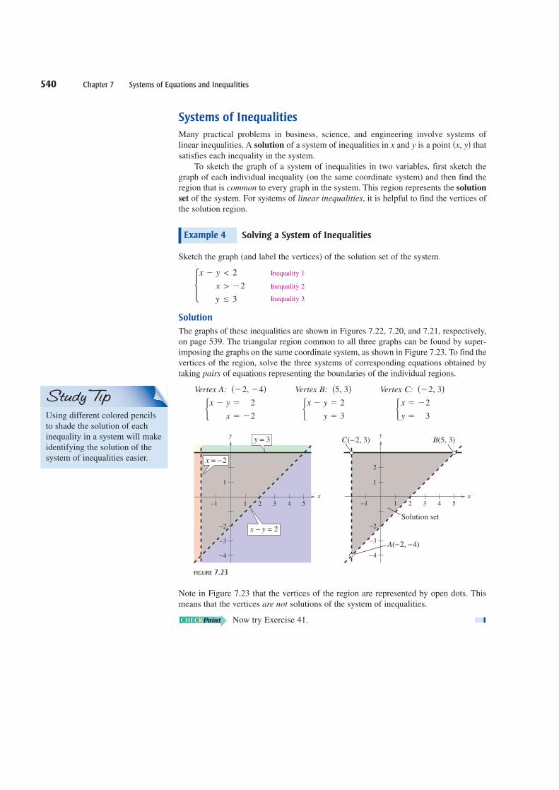
Solving a System of Inequalities

Sketch the graph (and label the vertices) of the solution set of the system.

Solution

The graphs of these inequalities are shown in Figures 7.22, 7.20, and 7.21, respectively,

on page 539. The triangular region common to all three graphs can be found by super-

imposing the graphs on the same coordinate system, as shown in Figure 7.23. To find the

vertices of the region, solve the three systems of corresponding equations obtained by

taking pairs of equations representing the boundaries of the individual regions.

Vertex A: Vertex B: Vertex C:

FIGURE 7.23

Note in Figure 7.23 that the vertices of the region are represented by open dots. This

means that the vertices are not solutions of the system of inequalities.


−1 1 2 3 4 5

1

2

−2

−3

−4

C(−2, 3)

A(−2, −4)

B(5, 3)

Solution set

y

x

−1 1 2 3 4 5

1

−2

−3

−4

x − y = 2

y = 3

x = −2

y

x

�x �y ��2

3�x � y �

y �

2

3�x � y �

x �

2

�2

��2, 3��5, 3��2, �4�

Inequality 1

Inequality 2

Inequality 3�x � y <

x >

y

2

�2

3

Example 4

�x, y�yx


Using different colored pencils

to shade the solution of each

inequality in a system will make

identifying the solution of the

system of inequalities easier.


For the triangular region shown in Figure 7.23, each point of intersection of a pair

of boundary lines corresponds to a vertex. With more complicated regions, two border

lines can sometimes intersect at a point that is not a vertex of the region, as shown in

Figure 7.24. To keep track of which points of intersection are actually vertices of the

region, you should sketch the region and refer to your sketch as you find each point of

intersection.

FIGURE 7.24

Solving a System of Inequalities

Sketch the region containing all points that satisfy the system of inequalities.

Solution

As shown in Figure 7.25, the points that satisfy the inequality

Inequality 1

are the points lying above (or on) the parabola given by

Parabola

The points satisfying the inequality

Inequality 2

are the points lying below (or on) the line given by

Line

To find the points of intersection of the parabola and the line, solve the system of

corresponding equations.

Using the method of substitution, you can find the solutions to be and

So, the region containing all points that satisfy the system is indicated by the shaded

region in Figure 7.25.


�2, 3�.��1, 0�

� x2� y � 1

�x � y � 1

y � x � 1.

�x � y 1

y � x2� 1.

x2� y 1

Inequality 1

Inequality 2� x2� y 1

�x � y 1

Example 5

Not a vertex

y

x

−2 2

1

2

3

(−1, 0)

(2, 3)

y = x2 − 1 y = x + 1

x

y

FIGURE 7.25

When solving a system of inequalities, you should be aware that the system might

have no solution or it might be represented by an unbounded region in the plane. These

two possibilities are shown in Examples 6 and 7.

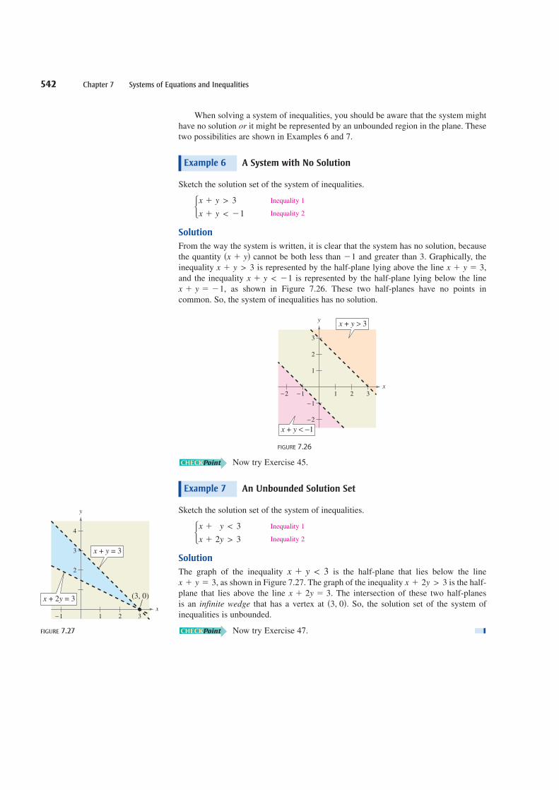
A System with No Solution

Sketch the solution set of the system of inequalities.

Solution

From the way the system is written, it is clear that the system has no solution, because

the quantity cannot be both less than and greater than 3. Graphically, the

inequality is represented by the half-plane lying above the line

and the inequality is represented by the half-plane lying below the line

as shown in Figure 7.26. These two half-planes have no points in

common. So, the system of inequalities has no solution.

FIGURE 7.26


An Unbounded Solution Set

Sketch the solution set of the system of inequalities.

Solution

The graph of the inequality is the half-plane that lies below the line

as shown in Figure 7.27. The graph of the inequality is the half-

plane that lies above the line The intersection of these two half-planes

is an infinite wedge that has a vertex at So, the solution set of the system of

inequalities is unbounded.


�3, 0�.x � 2y � 3.

x � 2y > 3x � y � 3,

x � y < 3

Inequality 1

Inequality 2�x � y < 3

x � 2y > 3

Example 7

−2 −1 1 2 3

1

2

3

−1

−2

x + y < −1

x + y > 3y

x

x � y � �1,

x � y < �1

x � y � 3,x � y > 3

�1�x � y�

Inequality 1

Inequality 2�x � y >

x � y <

3

�1

Example 6


x + 2y = 3

x + y = 3

−1 1 2 3

2

3

4

(3, 0)

x

y

FIGURE 7.27


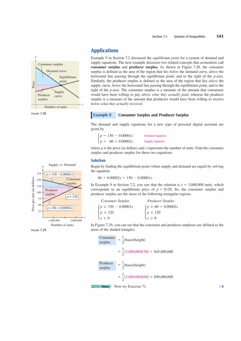
Applications

Example 9 in Section 7.2 discussed the equilibrium point for a system of demand and

supply equations. The next example discusses two related concepts that economists call

consumer surplus and producer surplus. As shown in Figure 7.28, the consumer

surplus is defined as the area of the region that lies below the demand curve, above the

horizontal line passing through the equilibrium point, and to the right of the -axis.

Similarly, the producer surplus is defined as the area of the region that lies above the

supply curve, below the horizontal line passing through the equilibrium point, and to the

right of the -axis. The consumer surplus is a measure of the amount that consumers

would have been willing to pay above what they actually paid, whereas the producer

surplus is a measure of the amount that producers would have been willing to receive

below what they actually received.

Consumer Surplus and Producer Surplus

The demand and supply equations for a new type of personal digital assistant are

given by

where is the price (in dollars) and represents the number of units. Find the consumer

surplus and producer surplus for these two equations.

Solution

Begin by finding the equilibrium point (when supply and demand are equal) by solving

the equation

In Example 9 in Section 7.2, you saw that the solution is units, which

corresponds to an equilibrium price of So, the consumer surplus and

producer surplus are the areas of the following triangular regions.

Consumer Surplus Producer Surplus

In Figure 7.29, you can see that the consumer and producer surpluses are defined as the

areas of the shaded triangles.

(base)(height)

(base)(height)


� $90,000,000�1

2�3,000,000��60�

�1

2

Producer

surplus

� $45,000,000�1

2�3,000,000��30�

�1

2

Consumer

surplus

�p � 60 � 0.00002x

p 120

x � 0�p 150 � 0.00001x

p � 120

x � 0

p � $120.

x � 3,000,000

60 � 0.00002x � 150 � 0.00001x.

xp

Demand equation

Supply equation�p � 150 � 0.00001x

p � 60 � 0.00002x

Example 8

p

p

Price

Number of units

Producer

surplus

Consumer surplus

Demand curve

Equilibrium

point

Supply

curve

x

p

FIGURE 7.28

Number of units

Price per unit (in dollars)

1,000,000 3,000,000

25

50

75

100

125

150

175

p

Producer

surplus

Consumer

surplus

p = 150 − 0.00001x

x

Supply vs. Demand

p = 120

p = 60 + 0.00002x

FIGURE 7.29

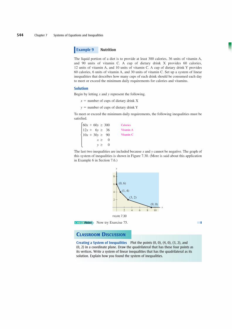
Nutrition

The liquid portion of a diet is to provide at least 300 calories, 36 units of vitamin A,

and 90 units of vitamin C. A cup of dietary drink X provides 60 calories,

12 units of vitamin A, and 10 units of vitamin C. A cup of dietary drink Y provides

60 calories, 6 units of vitamin A, and 30 units of vitamin C. Set up a system of linear

inequalities that describes how many cups of each drink should be consumed each day

to meet or exceed the minimum daily requirements for calories and vitamins.

Solution

Begin by letting and represent the following.

number of cups of dietary drink X

number of cups of dietary drink Y

To meet or exceed the minimum daily requirements, the following inequalities must be

satisfied.

The last two inequalities are included because and cannot be negative. The graph of

this system of inequalities is shown in Figure 7.30. (More is said about this application

in Example 6 in Section 7.6.)

FIGURE 7.30


2 4 6 8 10

2

4

6

8

(0, 6)

(1, 4)

(3, 2)

(9, 0)

y

x

yx

Calories

Vitamin A

Vitamin C�60x � 60y �

12x � 6y �

10x � 30y �

x �

y �

300

36

90

0

0

y �

x �

yx

Example 9


Creating a System of Inequalities Plot the points and in a coordinate plane. Draw the quadrilateral that has these four points as

its vertices. Write a system of linear inequalities that has the quadrilateral as itssolution. Explain how you found the system of inequalities.

0, 2! 3, 2!, 4, 0!, 0, 0!,

CLASSROOM DISCUSSION


EXERCISES See www.CalcChat.com for worked-out solutions to odd-numbered exercises.7.5

VOCABULARY: Fill in the blanks.

1. An ordered pair is a ________ of an inequality in and if the inequality is true when and are

substituted for and respectively.

2. The ________ of an inequality is the collection of all solutions of the inequality.

3. The graph of a ________ inequality is a half-plane lying on one side of the line

4. A ________ of a system of inequalities in and is a point that satisfies each inequality in the system.

5. A ________ ________ of a system of inequalities in two variables is the region common to the graphs of

every inequality in the system.

6. The area of the region that lies below the demand curve, above the horizontal line passing through the

equilibrium point, to the right of the -axis is called the ________ _________.

SKILLS AND APPLICATIONS

p

�x, y�yx

ax � by � c.

y,x

bayx�a, b�

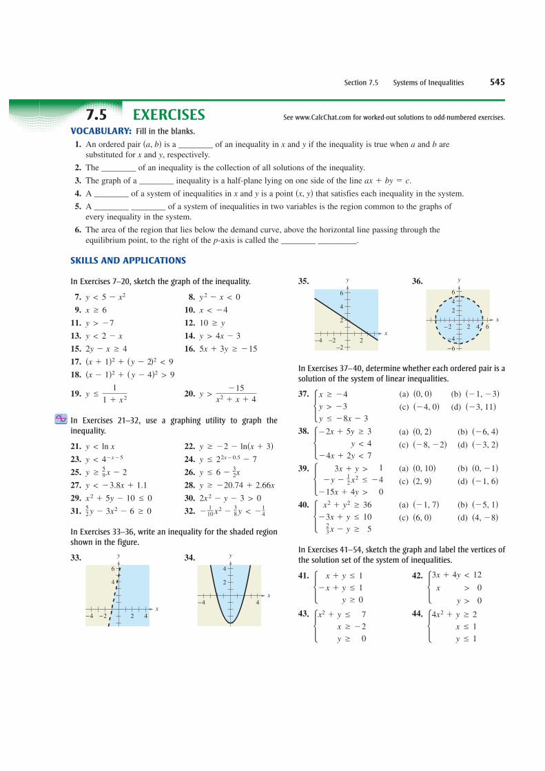
In Exercises 7–20, sketch the graph of the inequality.

7. 8.

9. 10.

11. 12.

13. 14.

15. 16.

17.

18.

19. 20.

In Exercises 21–32, use a graphing utility to graph the

inequality.

21. 22.

23. 24.

25. 26.

27. 28.

29. 30.

31. 32.

In Exercises 33–36, write an inequality for the shaded region

shown in the figure.

33. 34.

35. 36.

In Exercises 37–40, determine whether each ordered pair is a

solution of the system of linear inequalities.

37.

38.

39.

40.

In Exercises 41–54, sketch the graph and label the vertices of

the solution set of the system of inequalities.

41. 42.

43. 44.

�4x2 � y

x

y

� 2

1

1�x2 � y

x

y

�

�

7

�2

0

�3x

x

� 4y

y

<

>

>

12

0

0�

x � y 1

�x � y 1

y � 0

�x2 � y2 � 36

�3x � y 1023x � y � 5

�3x � y >

�y �12x

2

�15x � 4y >

1

�4

0

��2x � 5y � 3

y < 4

�4x � 2y < 7

�x � �4

y > �3

y �8x � 3

y

x

−2 2 4 6

−4

−6

2

4

6

2−2−2

−4

4

6

2

y

x

4−4

4

2

y

x

y

x

−2−4 2 4

4

6

�110x

2�

38y < �

14

52y � 3x2 � 6 � 0

2x2 � y � 3 > 0x2 � 5y � 10 0

y � �20.74 � 2.66xy < �3.8x � 1.1

y 6 �32xy �

59x � 2

y 22x�0.5 � 7y < 4�x�5

y � �2 � ln�x � 3�y < ln x

y >

�15

x2 � x � 4y

1

1 � x2

�x � 1�2 � � y � 4�2 > 9

�x � 1�2 � �y � 2�2 < 9

5x � 3y � �152y � x � 4

y > 4x � 3y < 2 � x

10 � yy > �7

x < �4x � 6

y2 � x < 0y < 5 � x2

(a) (b)

(c) (d) ��3, 11��4, 0��1, �3��0, 0�

(a) (b)

(c) (d) ��3, 2��8, �2��6, 4��0, 2�

(a) (b)

(c) (d) ��1, 6��2, 9��0, �1��0, 10�

(a) (b)

(c) (d) �4, �8��6, 0��5, 1��1, 7�

Partial Fraction Decomposition - unibo.itfioresi/2018/gen/lec5.pdf · Partial Fraction...

Documents

Transcript of Partial Fraction Decomposition - unibo.itfioresi/2018/gen/lec5.pdf · Partial Fraction...