Partial Differential Equations∗ (TATA27)

David Rule

Spring 2017

Contents

1 Preliminaries 21.1 Notation . . . . . . . . . . . . . . . . . . . . . . . . . . . . . . . . . . . . . . . . . . . . . 21.2 Differential equations . . . . . . . . . . . . . . . . . . . . . . . . . . . . . . . . . . . . . . 3

2 First-order linear equations and the method of characteristics 42.1 The method of characteristics . . . . . . . . . . . . . . . . . . . . . . . . . . . . . . . . . 4

3 The physical origins of some PDEs 63.1 Vibrations and the wave equation . . . . . . . . . . . . . . . . . . . . . . . . . . . . . . . 63.2 Diffusion and the heat equation . . . . . . . . . . . . . . . . . . . . . . . . . . . . . . . . 73.3 Harmonic functions . . . . . . . . . . . . . . . . . . . . . . . . . . . . . . . . . . . . . . . 8

4 Boundary value problems and well-posedness 84.1 Function spaces . . . . . . . . . . . . . . . . . . . . . . . . . . . . . . . . . . . . . . . . . 84.2 Initial conditions . . . . . . . . . . . . . . . . . . . . . . . . . . . . . . . . . . . . . . . . 84.3 Boundary conditions . . . . . . . . . . . . . . . . . . . . . . . . . . . . . . . . . . . . . . 94.4 Well-posedness . . . . . . . . . . . . . . . . . . . . . . . . . . . . . . . . . . . . . . . . . 9

5 Laplace’s and Poisson’s equation 105.1 A maximum principle . . . . . . . . . . . . . . . . . . . . . . . . . . . . . . . . . . . . . 105.2 Uniqueness for the Dirichlet Problem . . . . . . . . . . . . . . . . . . . . . . . . . . . . . 115.3 Laplace’s equation in two dimensions . . . . . . . . . . . . . . . . . . . . . . . . . . . . . 11

5.3.1 The Laplacian in polar coordinates . . . . . . . . . . . . . . . . . . . . . . . . . . 115.3.2 Poisson’s formula via separation of variables . . . . . . . . . . . . . . . . . . . . . 125.3.3 Mean Value Property and the Strong Maximum Principle . . . . . . . . . . . . . 14

5.4 Laplace’s equation in n dimensions . . . . . . . . . . . . . . . . . . . . . . . . . . . . . . 155.4.1 Green’s first identity . . . . . . . . . . . . . . . . . . . . . . . . . . . . . . . . . . 155.4.2 Mean Value Property and the Strong Maximum Principle . . . . . . . . . . . . . 165.4.3 Dirichlet’s Principle . . . . . . . . . . . . . . . . . . . . . . . . . . . . . . . . . . 165.4.4 Green’s second identity and the fundamental solution . . . . . . . . . . . . . . . 175.4.5 Green’s functions . . . . . . . . . . . . . . . . . . . . . . . . . . . . . . . . . . . . 185.4.6 Finding the Green’s function: the example of the upper half-plane . . . . . . . . 19

∗These lecture notes are a based on the book Partial Differential Equations by W.A Strauss.Last modified: 19th May 2017.

1

6 The wave equation 216.1 One spatial dimension: d’Alembert’s formula . . . . . . . . . . . . . . . . . . . . . . . . 216.2 Causality . . . . . . . . . . . . . . . . . . . . . . . . . . . . . . . . . . . . . . . . . . . . 226.3 Energy . . . . . . . . . . . . . . . . . . . . . . . . . . . . . . . . . . . . . . . . . . . . . . 246.4 Reflections . . . . . . . . . . . . . . . . . . . . . . . . . . . . . . . . . . . . . . . . . . . . 25

6.4.1 Waves on the half-line . . . . . . . . . . . . . . . . . . . . . . . . . . . . . . . . . 256.4.2 Waves on a finite interval . . . . . . . . . . . . . . . . . . . . . . . . . . . . . . . 26

6.5 Higher dimensions . . . . . . . . . . . . . . . . . . . . . . . . . . . . . . . . . . . . . . . 276.5.1 Three spatial dimensions: spherical means . . . . . . . . . . . . . . . . . . . . . . 276.5.2 Two spatial dimensions: the method of descent . . . . . . . . . . . . . . . . . . . 28

7 The heat equation 297.1 Another maximum principle . . . . . . . . . . . . . . . . . . . . . . . . . . . . . . . . . . 297.2 Uniqueness and stability via the energy method . . . . . . . . . . . . . . . . . . . . . . . 297.3 The initial value problem on the real line . . . . . . . . . . . . . . . . . . . . . . . . . . 307.4 A comparison of the wave and heat equations . . . . . . . . . . . . . . . . . . . . . . . . 327.5 The heat equation on a bounded interval . . . . . . . . . . . . . . . . . . . . . . . . . . . 33

8 Numerical analysis 348.1 Finite differences . . . . . . . . . . . . . . . . . . . . . . . . . . . . . . . . . . . . . . . . 348.2 Approximating solutions to the heat equation . . . . . . . . . . . . . . . . . . . . . . . . 35

8.2.1 An unstable scheme . . . . . . . . . . . . . . . . . . . . . . . . . . . . . . . . . . 358.2.2 A stability condition . . . . . . . . . . . . . . . . . . . . . . . . . . . . . . . . . . 368.2.3 The Crank-Nicolson Scheme . . . . . . . . . . . . . . . . . . . . . . . . . . . . . . 37

8.3 Approximations of Laplace’s equation . . . . . . . . . . . . . . . . . . . . . . . . . . . . 388.3.1 A discrete mean value property . . . . . . . . . . . . . . . . . . . . . . . . . . . . 388.3.2 The finite element method . . . . . . . . . . . . . . . . . . . . . . . . . . . . . . . 39

9 Schrodinger’s equation 419.1 The harmonic oscillator . . . . . . . . . . . . . . . . . . . . . . . . . . . . . . . . . . . . 419.2 The hydogen atom . . . . . . . . . . . . . . . . . . . . . . . . . . . . . . . . . . . . . . . 42

1 Preliminaries

1.1 Notation

You will be familiar with notation for derivatives from previous courses, in particular from Calculusand Multivariable Calculus, but let us refresh our memories.

Given a real-valued function g of one real variable (g : E → R where E ⊂ R), we denote thederivative of g at a point in the function’s domain x as

g′(t) = g(t) =dg

dt(t) := lim

h→0

g(t+ h)− g(t)

h.

For a function f of more than one real variable, say f : D → R where D ⊂ R3, we have threepossible partial derivatives and a menagerie of notation:

f ′x(x, y, z) = fx(x, y, z) = ∂1f(x, y, z) = ∂xf(x, y, z) =∂f

∂x(x, y, z) := lim

h→0

f(x+ h, y, z)− f(x, y, z)

h;

f ′y(x, y, z) = fy(x, y, z) = ∂2f(x, y, z) = ∂yf(x, y, z) =∂f

∂y(x, y, z) := lim

h→0

f(x, y + h, z)− f(x, y, z)

h;

f ′z(x, y, z) = fz(x, y, z) = ∂3f(x, y, z) = ∂zf(x, y, z) =∂f

∂z(x, y, z) := lim

h→0

f(x, y, z + h)− f(x, y, z)

h.

2

Different authors have different preferences and each notation seems best suited to different situations,so it’s good to be aware of them all.

Higher order derivates are denoted analogously, for example fxx, ∂x∂yf , ∂2f/∂y2, fxxy, etc.The vector formed of all the partial derivates of f is called the gradient of f . This is written

∇f := (∂1f, ∂2f, ∂3f)

For a function F : D → R3, we can consider the divergence of F :

divF = ∇ · F := ∂1F1 + ∂2F2 + ∂3F3,

where F = (F1, F2, F3). We can also consider the curl of F :

curlF = ∇× F := (∂2F3 − ∂3F2, ∂3F1 − ∂1F3, ∂1F2 − ∂2F1)

1.2 Differential equations

A differential equation is an equation that involves an unknown function u and derivatives of u. If uis a function of one variable, then the equation is called an ordinary differential equation (ODE). If uis a function of more than one variable, then the equation is a partial differential equation (PDE). Forexample, u′ = u is an ordinary diffential equation, but ux + 4uy = 0 is a partial differential equation.

A function u which satisfies a differential equation is called a solution to the equation. For exampleu(x) = ex is a solution to the equation u′ = u.

The order of a differential equation is the order of the highest derivative that appears in theequation. Thus all second-order partial differential equations in two variables takes the form

F (x, y, u, ∂xu, ∂yu, ∂xxu, ∂xyu, ∂yyu) = 0.

For example, if F (x, y, w0, w1, w2, w11, w12, w22) = w11 + w22, then the differential equation is ∂xxu +∂yyu = 0.

We will find the notion of differential operator convenient to use. An operator is a function whichmaps functions to functions. A differential operator which takes derivatives of the function it actson. For example, for a fixed n ∈ N, ∇ is a differential operator which maps f : Rn → R to thefunction ∇f : Rn → Rn given by the formula ∇f(x) = (∂1f(x), ∂2f(x), . . . , ∂nf(x)). It is oftenuseful to use the notation introduced above to denote differential operators, for example the operatoru 7→ ut − uxx = (∂t − ∂2

x)u can be denoted simply as (∂t − ∂2x).

An operator L is called linear if L(αu+ βv) = αL(u) + βL(v) for all α, β ∈ R and all functions uand v. It is easy to check the following operators are linear operators.

1. The gradient operator ∇ = (∂1, ∂2, . . . , ∂n) acting on functions u : Rn → R.

2. Divergence div acting on functions u : Rn → Rn as div u =∑n

j=1 ∂juj where uj : Rn → R arethe component functions of u so u = (u1, u2, . . . , un).

3. curl acting on functions u = (u1, u2, u3) : R3 → R3 by the formula

curl(u) = (∂2u3 − ∂3u2, ∂3u1 − ∂1u3, ∂1u2 − ∂2u1).

4. The Laplacian ∆ := ∇ · ∇ =∑n

j=1 ∂2j acting on f : Rn → R.

An example of an operator which is not linear is u 7→ uy + uxxy + uux. (Why?)The order of an operator is the order of the differential equation L(u) = 0 as an equation in u. A

differential equation is said to be a linear homogeneous equation, if it is of the form L(u) = 0, whereL is a linear differential operator. It is said to be a linear inhomogeneous equation if it is of the formL(u) = f for some function f , where again L is a linear differential operator.

3

2 First-order linear equations and the method of characteristics

We shall begin by attempting to solve a fairly simple equation: Find all functions u : R3 → R suchthat

aux + buy + cuz = 0 in R3, (2.1)

where a, b and c are three given constants not all zero. Although the equation itself is simple, to solveit we will use a method which is quite powerful. Observe that the equation can be rewritten as

v · ∇u = 0

where v = (a, b, c). Thus the equation says that the directional derivate in the direction v/|v| is zero.Thus any solution u will be constant along lines parallel to v.

(a) An example of a line along which a solu-tion u to (2.1) is constant.

(b) A characteristic curve along which a solu-tion u to (2.2) is constant

Figure 1: Characteristic curves

Since we are assuming that at least one of a, b and c is non-zero, suppose for definitness that c 6= 0.Then the vector v has a component pointing out of the xy-plane and each point (x, y, z) ∈ R3 lies on aunique line parallel to v which passes through the xy-plane at a point (x′, y′, 0) (see Figure 1(a)). Sincewe worked out that the solution u is constant along lines parallel to v, we know u(x, y, z) = u(x′, y′, 0).Moreover, the difference between (x, y, z) and (x′, y′, 0) is some multiple α ∈ R of v. That is,

(x, y, z)− (x′, y′, 0) = α(a, b, c).

Since c 6= 0, we have that α = z/c, so x′ = x− za/c and y′ = y − zb/c. Thus,

u(x, y, z) = u(x− za/c, y − zb/c, 0).

Finally, we observe that we are free to choose the value of the solution arbitrarily on the xy-plane, sothe general solution to (2.1) is of the form

u(x, y, z) = f(x− za/c, y − zb/c).

Such a u will solve equation (2.1) provided both first-order partial derivates of f : R2 → R exist.The cases when a 6= 0 and b 6= 0 can be handled similarly.

2.1 The method of characteristics

Now we have solved (2.1) we can see that the key was to identify lines along which the solution wasconstant. Let us take this idea but apply it in a more abstract setting to solve a similar, but morecomplicated equation, this time in two variables. Consider the equation

xuy(x, y)− yux(x, y) = 0 for (x, y) ∈ R2 \ (0, 0). (2.2)

4

This is again a first-order linear equation, but this time with variable coefficients. We will look forlines in R2 \ (0, 0) along which the solution u is constant. Suppose these lines are parametrised bya variable t and the x-coordinate is given by the function t 7→ X(t) and the y-coordinate by t 7→ Y (t).Thus we know that

t 7→ u(X(t), Y (t)) =: z(t) is a constant function

Consequently, using the chain rule, we have that

0 = z′(t) =d

dtu(X(t), Y (t)) = X ′(t)ux(X(t), Y (t)) + Y ′(t)uy(X(t), Y (t)). (2.3)

Comparing this with equation (2.2) we see that it is a good idea to choose

X ′(t) = −Y (t), and

Y ′(t) = X(t),

which have solutions X(t) = α cos(t) and Y (t) = α sin(t) for any α ∈ R (see Figure 1(b)). Thus anysolution to (2.2) is constant on circles centred at the origin and an arbitrary solution can be written inthe form

u(x, y) = f(x2 + y2).

Such a function will solve (2.2) provided f : (0,∞)→ R is differentiable. The curves

(x, y)|x = X(t), y = Y (t) for some t ∈ R

are called the characteristic curves (or more simply, the characteristics) of (2.2).The method we employed here was to search for curves (called characteristic curves) on which the

solution to our PDE behaved in a simple manner. In the previous two examples, the solution wasconstant on the characteristic curves, but, in principle, the solution only needed to behave in a way wecould understand easily—for example, it would suffice if t 7→ u(X(t), Y (t)) satisfied an ODE we couldeasily solve. Let us look at another which demonstrates this more complicated situation.

Consider the equation

ux(x, y) + cos(x)uy(x, y) = 1 for (x, y) ∈ R2 (2.4)

and suppose that we are given the value of u along the y-axis, say

u(0, y) = f(y) (2.5)

for some differentable function f : R → R and all y ∈ R. Once again we look for particular curvest 7→ (X(t), Y (t)) but instead of requiring z(t) := u(X(t), Y (t)) is constant along these curves, we allow(2.4) to determine how z behaves. Using the chain rule,

z′(t) =d

dtu(X(t), Y (t)) = X ′(t)ux(X(t), Y (t)) + Y ′(t)uy(X(t), Y (t)).

Comparing this with the coefficients in front of the first order terms in (2.4), we take

X ′(t) = 1, and (2.6)

Y ′(t) = cos(X(t)), (2.7)

which means z satisfies the ODE

z′(t) = ux(X(t), Y (t)) + cos(X(t))uy(X(t), Y (t)) = 1. (2.8)

The ODE (2.8) is a replacement for (2.3) in the previous example: z is not longer a constant function,where it satisfied z′(t) = 0, but instead satisfies a slightly more complicated ODE, z′(t) = 1, which wemust also solve.

5

First we find the characteristic curves. We can solve (2.6) to obtain X(t) = t+ c1 for a constant c1

and substituting this in (2.7), we have Y ′(t) = cos(t+c1), which implies Y (t) = sin(t+c1)+c2. We nowwant to relate the solution u(x, y) at an arbitrary point (x, y) with the solution at a point along they-axis, where we know the solution is equal to f by (2.5). So we look for a characteristic curve whichgoes through the point (x, y) when t = 0. This is easy to find: we take c1 = x and c2 = y − sin(x), so

X(t) = t+ x, and

Y (t) = sin(t+ x) + y − sin(x).

The curve t 7→ (X(t), Y (t) will intersect the y-axis when 0 = X(t) = t+ x, which occurs when t = −x.To relate u(x, y) with u(0, Y (−x)) we calculate

∫ 0−x z

′(t)dt. By the Fundamental Theorem of Calculus,∫ 0

−xz′(t)dt = z(0)− z(−x) = u(X(0), Y (0))− u(X(−x), Y (−x)) = u(x, y)− u(0, y − sin(x)),

but, using (2.8), this is also ∫ 0

−xz′(t)dt =

∫ 0

−x1dt = x,

so we obtain x = u(x, y)−u(0, y− sin(x)) = u(x, y)− f(y− sin(x)), where we also used (2.5), and thus

u(x, y) = x+ f(y − sin(x)).

We can check directly that this is indeed a solution to (2.4) and satisfies (2.5).The method of characteristics can be summarised as a method where we first look for particular

curves t 7→ (X(t), Y (t)) along which the solution to our PDE obeys a simple ODE — an ODE in theunknown z(t) = u(X(t), Y (t)) — and then solve this ODE. In the previous example, the characteristiccurves were determined by (2.6)-(2.7). Hopefully there are sufficiently many curves so that there isalways one connecting an arbitrary point (x, y) to a point where we have information about the solution(the y-axis in the previous example). We can then compare the solution at these two points by solvingthe ODE for z (this was the ODE (2.8) in our example).

3 The physical origins of some PDEs

In this section we will give some physical motivation for the main equations we will study. We willnot worry about being too careful in our derivation of the equations, but simply want to provide somephysical context for why the equations are of interest. Our careful mathematical analysis will now bepostponed until the next section, where we will take the equations as the starting point.

3.1 Vibrations and the wave equation

Let us consider a vibrating drumhead. Suppose that an elastic membrane is streached over a frame ∂Dthat lies in the xy-plane. For each point x inside the frame (a region D, so x ∈ D) and time t we denotethe displacement of the membrane by u(x, t). We wish to derive a simple equation that the function usatisfies in D which describes how the membrane behaves when subject to small displacements.

Assume the membrane has a mass density of ρ and is under constant tension (force per unitarclength) of magnitude T . Newton’s second law says that the mass times the acceleration of a smallpart of the membrane D′ is equal to the (vector) sum of the forces acting on that part. We will assumethe membrane only moves in the vertical direction, so we are interested in the sum of the vecticalcomponents of the forces acting on a part of the membrane. The force of tension acts parallel to thesurface of the membrane, so its vertical component at each point x ∈ ∂D′ is proportional to

(∂u/∂n)√1 + (∂u/∂n)2

≈ ∂u

∂nif (∂u/∂n) is small,

6

(a) The tension T acting on the edge of apiece of the membrane acts in a direction par-allel with both the tangent plane of the sur-face z = u(x, y) and the plane containing thenormal vector n to ∂D and the z-axis. Weassume |T| = T is constant.

(b) To compute the vertical component of thetension at a point on the edge, consider theslope of z = u(x, y) in the normal direction

n. This is equal to T (∂u/∂n)√1+(∂u/∂n)2

which is ap-

proximately T∂u/∂n when ∂u/∂n is small.

Figure 2: Tension acting on a small piece of an elastic membrane

where n is the outward unit normal to ∂D′ and ∂u/∂n = n · ∇u is the normal derivative of u. Theconstant of proportionality is the tension T , so the total vertical force is the “sum” of this around theboundary ∂D′: ∫

∂D′T∂u

∂n(x)dσ(x).

(See Figure 2.) Newton’s second law says this is equal to the mass times the acceleration of D′. Thus∫∂D′

T∂u

∂n(x)dσ(x) =

∫∫D′ρutt(x)dx.

The divergence theorem says ∫∂D′

T∂u

∂n(x)dσ(x) =

∫∫D′

div(T∇u(x))dx,

and so, ∫∫D′

div(T∇u(x))dx =

∫∫D′ρutt(x)dx.

Since D′ was arbitrary, we find that u satisfies

utt(x, t) = c2∆u(x, t) for all x ∈ D and t ∈ R, where c =√

Tρ . (3.1)

The equation in (3.1) is called the wave equation

3.2 Diffusion and the heat equation

Let us consider two fluids which together fill a container. We are interested in how these two fluidswill mix. Fick’s law of diffusion states that

the flow of a fluid is proportional to the gradient of its concentration.

Let u(x, t) be the concentration of one fluid at a point x and time t. For an arbitrary region D′ themass of the fluid in D′ is

m(t) =

∫∫∫D′u(x, t)dx, so

dm

dt(t) =

∫∫∫D′ut(x, t)dx.

7

The rate of change of mass of fluid in the region D′ is also equal to the net flow of mass into the regionD′. By Fick’s law this is given by

dm

dt(t) =

∫∫∂D′

kn · ∇u(x, t)dσ(x).

Therefore using the divergence theorem, we obtain∫∫∫D′

div(k∇u)(x, t)dx =

∫∫∂D′

kn · ∇u(x, t)dσ(x) =dm

dt(t) =

∫∫∫D′ut(x, t)dx.

Once again, since D′ was abitrary, the integrands must also be equal:

ut(x, t) = k∆u(x, t) for all x and t. (3.2)

Equation (3.2) is called the diffusion or heat equation.

3.3 Harmonic functions

When we consider solutions to both the heat and the wave equation ((3.2) and (3.1)) which areindependent of time, we find that they are both solutions to Laplace’s equation:

∆u(x) =n∑j=1

∂2j u(x) = 0 (3.3)

Functions u which are solutions of (3.3) are called harmonic functions. When n = 1, the only suchfunctions are linear functions u(x) = kx+ c, but for n > 1 things become more interesting.

4 Boundary value problems and well-posedness

We have derived several different PDEs which model various physical situations, but we have also seenthat there can be many different solutions to any one given PDE. If a PDE is to be a genuinely usefulmodel, we would expect it to give exactly one possibility for a physical property (which the solution tothe PDE represents). Thus, we must add some further conditions to the model that will pick out thesolution which is physically relevant to a given situation. The precise conditions we have to add varyslightly depending on the model, but are usually motivated by physical considerations.

4.1 Function spaces

The function space where we look for a solution is a subtle issue, but important. For example, inquantum mechanics a solution u : R3 ×R→ C to a PDE can be connected to the probability densityof a particle. The probability that a particle lies in a region D ⊂ R3 at time t is given by∫

D|u(x, t)|2dx.

Since it is a probability, we would expect∫R3 |u(x, t)|2dx = 1, and so any physically reasonable solution

u is such that∫R3 |u(x, t)|2dx = 1 for all t.

4.2 Initial conditions

An initial condition specifies the solution at a particular instant of time. We typically use the variablesx = (x, y, z) to denote spatial coordinates and t to denote a time coordinate. So an initial conditioncan take the form u(x, t0) = f(x) for all x ∈ Rn (and a given f). We would then search for a solutionu which satisfies a given PDE for t > t0. If we consider heat flow (or diffusion of a chemical), specifyingthe temperature (or concentration) at a specific time t = t0, that is prescribing the solution u(·, t0) attime t0, ought to be sufficient to pin down a unique solution u(·, t) for t > t0. Thus, the problem we

8

expect to be able to solve is, given a function f : R3 → R, to find a unique function u : R× [t0,∞)→ Rsuch that

∂tu(x, t)− k∆u(x, t) = 0 for (x, t) ∈ R3 × (t0,∞), andu(x, t0) = f(x) for x ∈ R3.

Observe that here the function space we assume u to lie in is also important. For example, if we do notrequire that u is continuous at t = t0, the initial condition will not really limit the number of solutionswe have. It can be useful to reformulate the initial condition to take the need for such continuity intoaccount directly. For example,

limt→t0

u(x, t) = f(x) for all x ∈ R3.

Sometimes it is reasonable to give two initial conditions, as is the case with the wave equation.Given f : R3 → R and g : R3 → R, we expect to find a unique u : R3 × [t0,∞)→ R such that

∂2t u(x, t)− c2∆u(x, t) = 0 for (x, t) ∈ R3 × (t0,∞), andu(x, t0) = f(x) and ∂tu(x, t0) = g(x) for x ∈ R3.

Here the initial conditions specify the position and velocity of u at time t0.

4.3 Boundary conditions

Figure 3: A cup with an uneven rim sitting on a table.

A boundary condition specifies the value of a solution on the boundary of (what physically is) aspatial domain. For example, take a cup which has an uneven rim, place it on a table and then stretcha rubber sheet over its rim (see Figure 3). One can show that the height of the rubber should roughlybe given by a harmonic function (with respect to two variables — those of horizontal position over thetable) and the height at the boundary would, of course, be the height of the rim. Thus, if D is (theinterior of) the region of the table over which the cup sits, we would expect to be able to find a uniqueu : R2 → R such that

∆u(x, y) = 0 for all (x, y) ∈ D, andu(x, y) = f(x, y) for (x, y) ∈ ∂D.

Here ∂D denotes the boundary of D, that is, points above which the cup’s rim sits, and f(x, y) is theheight of the cup’s rim above the table at (x, y) ∈ ∂D.

4.4 Well-posedness

Once we believe we have formulated a physically sensible model, we then want to prove rigorously thefollowing properties.

1. Existence: There exists at least one solution that satisfies the PDE together with the ini-tial/boundary conditions and lies in our chosen function space.

9

2. Uniqueness: There exists at most one solution that satisfies the PDE together with the ini-tial/boundary conditions and lies in our chosen function space.

3. Stability: The solution depends continuously on the data (that is, the initial/boundary condi-tions).

We impose the third condition as in practice we cannot measure our data exactly, so it is useful toknow that any small error in measurement will only lead to a small change in the solution.

5 Laplace’s and Poisson’s equation

We said earlier that a solution to Laplace’s equation (3.3) is called harmonic. We will also be interestedin an inhomogeneous version of Laplace’s equation. Namely, Poisson’s equation:

∆u(x) =n∑j=1

∂2j u(x) = f(x) (5.1)

for a given function f .

5.1 A maximum principle

Maximum principles are very powerful analytic tool for studying harmonic functions. Recall that a setD ⊂ Rn is called open if for every point x ∈ D, there exists an ε > 0 such that the set y | |x−y| < εis a subset of D. A set D ⊂ Rn is called bounded if there exists a constant C > 0 such that |x| < Cfor all x ∈ D.

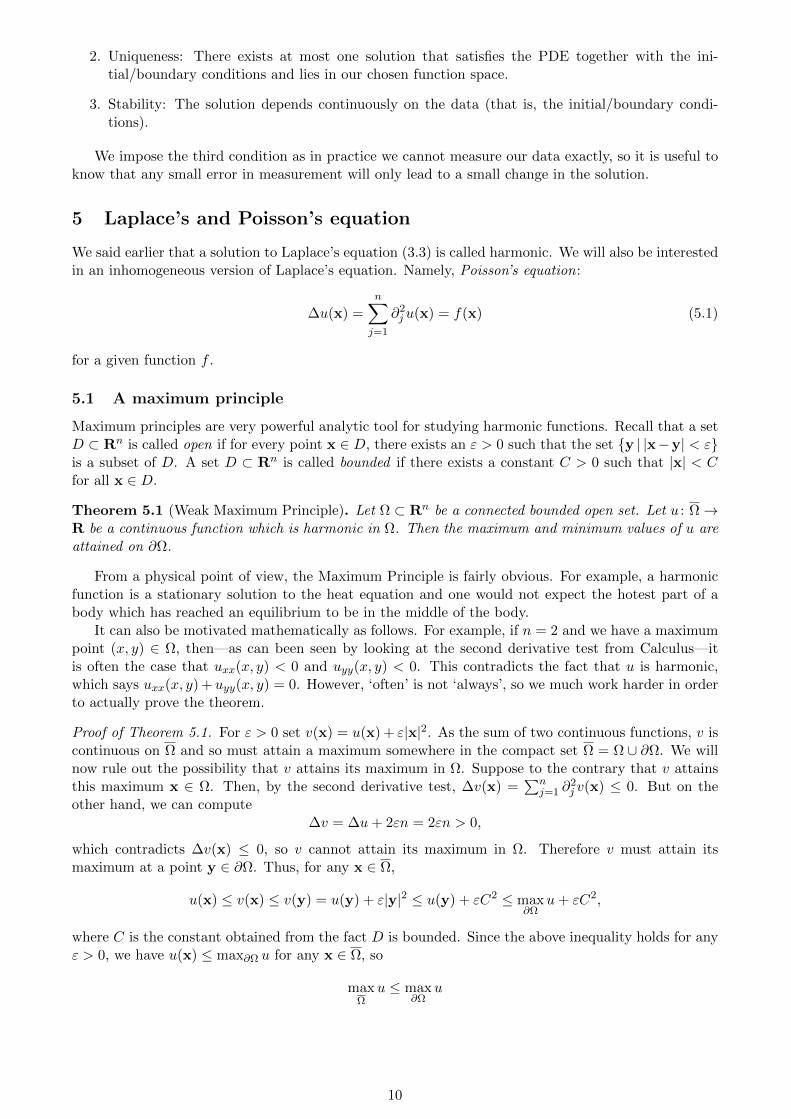
Theorem 5.1 (Weak Maximum Principle). Let Ω ⊂ Rn be a connected bounded open set. Let u : Ω→R be a continuous function which is harmonic in Ω. Then the maximum and minimum values of u areattained on ∂Ω.

From a physical point of view, the Maximum Principle is fairly obvious. For example, a harmonicfunction is a stationary solution to the heat equation and one would not expect the hotest part of abody which has reached an equilibrium to be in the middle of the body.

It can also be motivated mathematically as follows. For example, if n = 2 and we have a maximumpoint (x, y) ∈ Ω, then—as can been seen by looking at the second derivative test from Calculus—itis often the case that uxx(x, y) < 0 and uyy(x, y) < 0. This contradicts the fact that u is harmonic,which says uxx(x, y) + uyy(x, y) = 0. However, ‘often’ is not ‘always’, so we much work harder in orderto actually prove the theorem.

Proof of Theorem 5.1. For ε > 0 set v(x) = u(x) + ε|x|2. As the sum of two continuous functions, v iscontinuous on Ω and so must attain a maximum somewhere in the compact set Ω = Ω ∪ ∂Ω. We willnow rule out the possibility that v attains its maximum in Ω. Suppose to the contrary that v attainsthis maximum x ∈ Ω. Then, by the second derivative test, ∆v(x) =

∑nj=1 ∂

2j v(x) ≤ 0. But on the

other hand, we can compute∆v = ∆u+ 2εn = 2εn > 0,

which contradicts ∆v(x) ≤ 0, so v cannot attain its maximum in Ω. Therefore v must attain itsmaximum at a point y ∈ ∂Ω. Thus, for any x ∈ Ω,

u(x) ≤ v(x) ≤ v(y) = u(y) + ε|y|2 ≤ u(y) + εC2 ≤ max∂Ω

u+ εC2,

where C is the constant obtained from the fact D is bounded. Since the above inequality holds for anyε > 0, we have u(x) ≤ max∂Ω u for any x ∈ Ω, so

maxΩ

u ≤ max∂Ω

u

10

Because ∂Ω ⊆ Ω we have that max∂Ω u ≤ maxΩ u and combining these two inequalities we get thatmaxΩ u = max∂Ω u and the maximum of u is attained on ∂Ω. (Observe that we have not ruled out thepossibility that the maximum of u is also attained in Ω — that we only managed to do for v — so itmay still be possible that the maximum of u is attained both in Ω and on ∂Ω.)

That the minimum is attained on the boundary ∂Ω can be proved similarly.

5.2 Uniqueness for the Dirichlet Problem

We can use the Weak Maximum Principle to prove that a solution to the Dirichlet Problem for thePoisson equation is unique.

Suppose we had two functions u1 and u2 which where continuous on Ω, for an connected boundedopen set Ω ⊂ Rn and such that (for i = 1, 2)

∆ui = f in Ω, andui = g on ∂Ω,

(5.2)

where g : ∂Ω→ R and f : Ω→ R.The difference w := u2 − u1 is continuous on Ω and satisfies

∆w = 0 in Ω, andw = 0 on ∂Ω,

We can apply Theorem 5.1 to conclude that both the maximum and the minimum of w are obtainedon the boundary of ∂Ω, but by the boundary condition we know

0 = min∂Ω

w ≤ w(x) ≤ max∂Ω

w = 0

for any x ∈ Ω. Thus w ≡ 0 and so u1 = u2, that is to say, there is at most one continuous solutionu : Ω→ R of the boundary value problem

∆u = f in Ω, andu = g on ∂Ω,

for g : ∂Ω → R and f : Ω → R. Observe that we did not need to make any regularity assumptionsabout f or g, although obviously g may inherit continuity from the fact we assumed u was continuous.

5.3 Laplace’s equation in two dimensions

To further investigate the properties of harmonic functions it is instructive to first restrict our attentionto n = 2, so ∆ = ∂2/∂x2 + ∂2/∂y2.

5.3.1 The Laplacian in polar coordinates

We wish to use polar coordinates to rewrite the Laplace operator (Laplacian) in terms of ∂/∂r and∂/∂θ. The transformation from polar to Cartesian coordinates is given by

x = r cos θ and y = r sin θ

and the inverse is1

r =√x2 + y2 and θ = arctan(y/x)

Recall that the chain rule says

∂

∂x=∂r

∂x

∂

∂r+∂θ

∂x

∂

∂θand

∂

∂y=∂r

∂y

∂

∂r+∂θ

∂y

∂

∂θ

1The formula θ = arctan(y/x) is not quite the inverse, as θ may lie outside the range (−π/2, π/2).

11

so we obtain∂

∂x= cos θ

∂

∂r+

sin θ

r

∂

∂θand

∂

∂y= sin θ

∂

∂r+

cos θ

r

∂

∂θ

Squaring these operators, we obtain

∂2

∂x2=

(cos θ

∂

∂r+

sin θ

r

∂

∂θ

)2

= cos2 θ∂2

∂r2− 2

(sin θ cos θ

r

)∂2

∂r∂θ+

sin2 θ

r2

∂2

∂θ2+

(sin θ cos θ

r2

)∂

∂θ+

sin2 θ

r

∂

∂r

and

∂2

∂y2=

(sin θ

∂

∂r+

cos θ

r

∂

∂θ

)2

= sin2 θ∂2

∂r2+ 2

(sin θ cos θ

r

)∂2

∂r∂θ+

cos2 θ

r2

∂2

∂θ2−(

sin θ cos θ

r2

)∂

∂θ+

cos2 θ

r

∂

∂r.

These combine to give

∆ =∂2

∂x2+

∂2

∂y2=

∂2

∂r2+

1

r

∂

∂r+

1

r2

∂2

∂θ2.

We will use this in the next section to compute an explicit formula for solving Laplace’s equation inthe disc.

5.3.2 Poisson’s formula via separation of variables

Let D = x | |x| < a denote the disc of radius a > 0. We wish to solve the boundary-value problem∆u = 0 in D, and

u = h on ∂D,(5.3)

We will write u in polar coordinates, so Laplace’s equation becomes

∂2u

∂r2(r, θ) +

1

r

∂u

∂r(r, θ) +

1

r2

∂2u

∂θ2(r, θ) = 0

for 0 < r < a and θ ∈ [0, 2π), and the boundary condition can be written u(a, θ) = h(θ) :=h(a cos θ, a sin θ).

We will search for solutions of the form u(r, θ) = R(r)Θ(θ), a technique which is called separationof variables and is something we will use several times in the course. The equation becomes

R′′Θ +1

rR′Θ +

1

r2RΘ′′ = 0

Multiplying by r2/RΘ, we haver2R′′

R+rR′

R+

Θ′′

Θ= 0.

Observe that the first and second terms only depend on r and the third term only on θ. Consequently(why?) we obtain two separate ODEs:

Θ′′ + λΘ = 0 and r2R′′ + rR′ − λR = 0,

for λ ∈ R. These can be easily solved. We must ensure that Θ is periodic: Θ(θ+2π) = Θ(θ) for θ ∈ R.Thus

λ = m2 and Θ(θ) = Am cos(mθ) +Bm sin(mθ) (m = 0, 1, 2, . . . ).

for Am, Bm ∈ R. The equation for R is of Euler type, so we can search for solutions of the formR(r) = rα. Substituting this ansatz and λ = m2 into the equation for R we find that α = ±m and

R(r) = Cmrm +Dmr

−m (m = 1, 2, 3, . . . ) and R(r) = C0 +D0 ln r (m = 0)

12

for Cm, Dm ∈ R. (The logarithmic solution must be obtained by other means.)It seems unreasonable to allow solutions which are not continuous near the origin, so we reject

these, which amounts to taking Dm = 0 for all m = 0, 1, 2, . . . . Thus we are left with a number ofpossible solutions u(r, θ) = R(r)Θ(θ) indexed by a non-negative integer m:

Cmrm(Am cos(mθ) +Bm sin(mθ)) (m = 0, 1, 2, . . . ).

It is of course redundant to have the products CmAm and CmBm of two constants in each term, so weset Cm = 1 for m > 0 and C0 = 1/2. Why we make this specific choice will become clear when wechoose Am and Bm. Finally, in order to build a solution that matches the boundary condition from(5.3), u = h on ∂D, we consider linear combinations of these solutions:

u(r, θ) =1

2A0 +

∞∑m=1

rm(Am cos(mθ) +Bm sin(mθ)) (5.4)

The boundary condition can thus be rewritten as

h(θ) =1

2A0 +

∞∑m=1

am(Am cos(mθ) +Bm sin(mθ)),

which is exactly the Fourier series of h. Thus we choose Am and Bm to be the Fourier coefficients of h:

Am =1

πam

∫ 2π

0h(φ) cos(mφ)dφ and Bm =

1

πam

∫ 2π

0h(φ) sin(mφ)dφ. (5.5)

So we have found a representation, (5.4) and (5.5), of a solution to (5.3) provided the Fourier series ofh converges to h. However, we can significantly simplify the representation.

Substituting (5.5) in (5.4) we find that

u(r, θ) =

∫ 2π

0h(φ)

dφ

2π+

∞∑m=1

rm

πam

∫ 2π

0h(φ) (cos(mφ) cos(mθ) + sin(mφ) sin(mθ)) dφ

=

∫ 2π

0h(φ)

(1 + 2

∞∑m=1

(ra

)mcos(m(θ − φ))

)dφ

2π.

But (1 + 2

∞∑m=1

(ra

)mcos(m(θ − φ))

)= 1 +

∞∑m=1

(ra

)meim(θ−φ) +

∞∑m=1

(ra

)me−im(θ−φ)

= 1 +rei(θ−φ)

a− rei(θ−φ)+

re−i(θ−φ)

a− re−i(θ−φ)

=a2 − r2

a2 − 2ar cos(θ − φ) + r2.

Thus, our formula becomes

u(r, θ) =(a2 − r2)

2π

∫ 2π

0

h(φ)

a2 − 2ar cos(θ − φ) + r2dφ. (5.6)

This, in turn, can be simplified to

u(x) =(a2 − |x|2)

2πa

∫|y|=a

h(y)

|x− y|2dσ(y), (5.7)

where dσ(y) = adφ is arc-length measure and h(y) = h(φ) for y = (a cosφ, a sinφ). (See homeworkexercise 3.1.) Formulae (5.6) and (5.7) are two different forms of what is called the Poisson formulafor the solution to (5.3). The kernel

K(x,y) =(|y|2 − |x|2)

2π|y|1

|x− y|2

13

is called the Poisson kernel for the disc of radius a.In our derivation of the Poisson formula, we assumed that the Fourier series of h converged to h.

However, formulae (5.6) and (5.7) can be shown to solve (5.3) when h is just continuous. (Recall thatthere exist continuous functions for which the Fourier series diverges at a point, and thus does notconverge to the function.) We will not prove this last step, but just state it as a theorem.

Theorem 5.2. Let D = x | |x| < a be the disc of radius a and let h : ∂D → R be a continuousfunction. Then there exists a unique continuous function u : D → R which solves (5.3). This functionu is smooth in D (see Lemma 5.5 below) and given by (5.7) (or equally by (5.6) in polar coordinates,with h(θ) = h(a cos θ, a sin θ)).

5.3.3 Mean Value Property and the Strong Maximum Principle

Poisson’s formula has the following applications.

Theorem 5.3 (Mean Value Property in R2). Let Ω ⊂ R2 be an open set and u : Ω → R harmonic.Then for any disc Da(x) = y ∈ R2 | |y − x| < a such that D ⊂ Ω we have that

u(x) =1

2πa

∫∂Da(x)

u(y)dσ(y).

That is, the value of u at the centre of a disc is equal to the mean value of u over the boundary of thedisc.

Proof. By a change of variables and homework exercise 2.3, it suffices to prove the theorem whenx = 0 is the origin and so Da(x) = D from (5.3). We define a function h : ∂D → R by h(y) = u(y) fory ∈ ∂D. Since we proved there is only one continuous solution to (5.3), we know u is given by (5.7) inD. Thus, in particular,

u(0) =(a2 − |0|2)

2πa

∫|y|=a

h(y)

|0− y|2dσ(y)

=a2

2πa

∫|y|=a

u(y)

a2dσ(y)

=1

2πa

∫∂Ba(0)

u(y)dσ(y)

The Mean Value Theorem confirms something we would expect from the physical situations har-monic functions represent. It also has the following corollary. Recall that a set Ω ⊂ Rn is (path)connected if for every pair of points x,y ∈ D, there exists a continuous function γ : [0, 1] → D suchthat γ(0) = x and γ(1) = y.

Corollary 5.4 (Strong Maximum Principle in R2). Let Ω ⊂ R2 be a connected bounded open set. Letu : Ω→ R be a continuous function which is harmonic in Ω. Then if the maximum or minimum valuesof u are attained in Ω, then u is a constant function.

Proof. Suppose the maximum M is attained at a point x ∈ Ω, so u(x) = M , and that u is not constant,so there exists a y ∈ Ω such that u(y) < M . In fact, because u is continuous, we can assume y ∈ Ω.Since Ω is connected, there exists a curve in Ω from x to y (see Figure 4). Since u is continuous, thereexists a point z furthest along the curve towards y such that u(z) = M . Since Ω is open, we can finda sufficiently small a > 0 such that Da(z) ⊂ Ω. By the Mean Value Property,

M = u(z) =1

2πa

∫∂Da(z)

u(w)dσ(w).

14

Figure 4: The existence of w contradicts the fact z is taken to be the last point along the curve whichattains the maximum value M .

Therefore, since u(w) ≤ M , we must have u(w) = M for all w ∈ ∂Da(z), in particular we can find aw further along the curve such that u(w) = M . This contradicts the fact z was the last such point.

Therefore, either the maximum is not attained in Ω or u is constant. A similar argument provesthe statement for the minimum value.

Lemma 5.5. Let Ω ⊂ R2 be an open set and u : Ω → R harmonic. Then u possesses all partialderivatives of all orders (such a function is called smooth).

Proof. By a change of variables and homework exercise 2.3, we may assume 0 ∈ Ω and it suffices toprove u has all partial derivatives at the origin 0. Using the Poisson formula, we have an formula foru in a neighbourhood of the origin and it is easy to check this formula can be differentiated as manytimes as we wish.

5.4 Laplace’s equation in n dimensions

5.4.1 Green’s first identity

Suppose Ω ⊂ Rn is an open set with a C1-boundary.2 Suppose further that we have two functionsu ∈ C2(Ω) and v ∈ C1(Ω). The product rule tells us that

∂j(v∂ju) = ∂vj∂uj + v∂2j u

for each j = 1, 2, . . . , n. So∇ · (v∇u) = ∇v · ∇u+ v∆u.

Applying the divergence theorem, we find∫∂Ωv∂u

∂ndσ =

∫Ω

(∇v · ∇u+ v∆u)dV, (5.8)

where ∂u/∂n = n · ∇u and n is the outward unit normal to ∂Ω. Equation (5.8) is called Green’s firstidentity.

2This means that ∂Ω can be written as the union of a finite number of sets, each of which is the graph of a C1 functionwith respect to a choice of coordinates. More precisely, there exist a positive integer N such that for each i = 1, 2, . . . , Nthere exists an open set Ui ⊂ Rn−1, a matrix Ai whose rows form an orthonormal basis for Rn, and a C1 function fisuch that ∂Ω = y ∈ Rn |y = (x, fi(x))Ai for some i and x ∈ Ui

15

5.4.2 Mean Value Property and the Strong Maximum Principle

We have the following applications of Green’s first identity (5.8), which generalise the results we provedearlier when n = 2. Observe that we are required to strengthen our assumptions on u, as we havenot proved that a harmonic function of more than two variables is smooth. However, by being carefulabout we apply Green’s first identity, we can avoid the need to assume ∂Ω in the statements below isC1.

Theorem 5.6 (Mean Value Property in Rn, n ∈ N). Let Ω ⊂ Rn be an open set and let u : Ω → Rbe a C2 harmonic function. Then for any ball Ba(x) = y ∈ Rn | |y−x| < a such that Ba(x) ⊂ Ω wehave that

u(x) =1

ωn−1an−1

∫∂Ba(x)

u(y)dσ(y).

That is, the value of u at the centre of a ball is equal to the mean value of u over the boundary of theball.

Proof. We can apply Green’s first identity to the functions u as in the statement of the theorem, v ≡ 1and Ω = Ba(x). We find that ∫

∂Ba(x)

∂u(y)

∂ndσ(y) = 0.

Dividing by the area of ∂Ba(x), which is a constant ωn−1 times an−1, we have

0 =1

ωn−1an−1

∫∂Ba(x)

∂u(y)

∂ndσ(y) =

1

ωn−1

∫∂B1(0)

z · ∇u(x + az)dσ(z) =1

ωn−1

∫∂B1(0)

∂u(x + az)

∂adσ(z)

=1

ωn−1

d

da

∫∂B1(0)

u(x + az)dσ(z) =d

da

(1

ωn−1an−1

∫∂Ba(x)

u(y)dσ(y)

).

Thus, the quantity in parenthesis on the right-hand side above is constant. Taking the limit a→ 0 wesee that this constant must be u(x), which proves the theorem.

Once again, we can use the mean value property to prove a maximum principle.

Corollary 5.7 (Strong Maximum Principle in Rn, n ∈ N). Let Ω ⊂ Rn be a connected bounded openset. Let u : Ω→ R be a continuous function which is of class C2 and harmonic in Ω. If the maximumor minimum values of u are attained in Ω, then u is a constant function.

Proof. The proof of this is identical to that of Corollary 5.4.

5.4.3 Dirichlet’s Principle

We can now demonstrate an important idea which connects harmonic functions to a notion of energy(borrowed directly from physics). It states that amongst all (reasonably smooth) functions w : Ω→ Rwith a given boundary value w = h on ∂Ω, a function u which solves

∆u = 0 in Ω, andu = h on ∂Ω,

(5.9)

should minimise some sort of ‘energy’. We now state this idea more precisely.

Theorem 5.8. Suppose that Ω ⊂ Rn is a connected bounded open set with a C1 boundary ∂Ω and h isa C1 function defined on ∂Ω. For any C1 function w : Ω → R such that w(x) = h(x) for all x ∈ ∂Ω,define

E[w] =1

2

∫Ω|∇w|2.

Then a solution u ∈ C1(Ω) to (5.9) which is C2 in Ω is such that

E[u] ≤ E[w]

for any w as above.

16

Proof. Given u and w as above, observe that v := w − u is such that v(x) = 0 for all x ∈ ∂Ω. We canthen compute

2E[w] =

∫Ω|∇v +∇u|2 =

∫Ω

(|∇v|2 + |∇u|2 + 2∇v · ∇u) =

(∫Ω|∇v|2

)+ 2E[u] + 2

∫Ω∇v · ∇u.

Applying Green’s first identity (5.8), we see that∫Ω∇v · ∇u =

∫∂Ωv∂u

∂ndσ −

∫Ωv∆u = 0.

Thus E[w] ≥ E[u] since∫

Ω |∇v|2 ≥ 0.

5.4.4 Green’s second identity and the fundamental solution

In homework exercise 3.3 we used Green’s first identity (5.8) to prove Green’s second identity: Green’ssecond identity states that for two functions u, v ∈ C2(Ω)∫

Ωu(x)∆v(x)− v(x)∆u(x)dx =

∫∂Ωu(x)

∂v

∂n(x)− v(x)

∂u

∂n(x)dσ(x). (5.10)

We also considered the function Φ: Rn \ 0 → R defined by

Φ(x) =

− 1

2α(2) ln |x| if n = 2,1

n(n−2)α(n)1

|x|n−2 if n > 2,(5.11)

where α(n) is the volume of the unit ball in Rn. The function Φ is called the fundamental solution ofthe Laplace operator. We proved Φ was harmonic in Rn \ 0 and

∂Φ

∂n(x) =

−1

nα(n)

1

|x|n−1(5.12)

for each n = 2, 3, . . . in homework exercise 3.4.We can use these facts to prove the following lemma.

Lemma 5.9. Let Ω be an open bounded set with C1 boundary and suppose that u ∈ C2(Ω) is harmonicin Ω. Then

u(x) =

∫∂Ω

Φ(y − x)

(∂u

∂n

)(y)−

(∂Φ

∂n

)(y − x)u(y)

dσ(y). (5.13)

for each x ∈ Ω

Proof. We wish to apply Green’s second identity (5.10) to the functions Φ(· − x) and u in Ω. Howeverwe cannot as Φ(· − x) is not defined at x. We instead apply (5.10) to Ωr := Ω \Br(x). We obtain

0 =

∫∂Ωr

Φ(y − x)

(∂u

∂n

)(y)−

(∂Φ

∂n

)(y − x)u(y)

dσ(y).

However, ∂Ωr has two components, ∂Ω and ∂Br(x). The integral over ∂Ω is exactly the right-handside of (5.13), so we only need to calculate the integral over ∂Br(x). From (5.11) it is clear that Φ isa radial function—that is, we can write Φ(x) = φ(|x|) for

φ(r) =

− 1

2α(2) ln |r| if n = 2,1

n(n−2)α(n)1

rn−2 if n > 2.

Remembering that the outward normal n to Ωr is actually an inward normal to Br(x) on ∂Br(x), wehave from (5.12) that

∂Φ

∂n(y − x) =

1

nα(n)

1

rn−1.

17

Thus ∫∂Br(x)

Φ(y − x)

(∂u

∂n

)(y)−

(∂Φ

∂n

)(y − x)u(y)

dσ(y)

=

∫∂Br(x)

φ(r)

(∂u

∂n

)(y)dσ(y)−

∫∂Br(x)

1

nα(n)

1

rn−1u(y)dσ(y)

=φ(r)

(∫∂Br(x)

(∂u

∂n

)(y)dσ(y)

)−

(1

nα(n)rn−1

∫∂Br(x)

u(y)dσ(y)

).

Applying the divergence theorem (with −n being the outward unit normal), we see that(∫∂Br(x)

(∂u

∂n

)(y)dσ(y)

)= −

∫Br(x)

∆u(y)dy = 0.

Since nα(n)rn−1 is the surface area of ∂Br(x),3 the mean value property (Lemma 5.6) says(1

nα(n)rn−1

∫∂Br(x)

u(y)dσ(y)

)= u(x).

Putting these facts together, we see the lemma is proved.

5.4.5 Green’s functions

At first sight (5.13) appears to be a useful formula, as it expresses a harmonic function in a domainΩ in terms of its behaviour on the boundary ∂Ω. However, physically we do not expect to have tospecify both the value of u and the value of ∂u/∂n on the boundary. Therefore we wish to modify thefundamental solution (5.11) somewhat to eliminate one of the terms in (5.13).

To be more precise, suppose we wanted to solve the same boundary value problem we consideredin Section 5.4.3:

∆u = 0 in Ω, andu = h on ∂Ω.

(5.9)

If we can find a modification G of Φ which has very similar properties to Φ but is also zero on theboundary, then we should be able to solve (5.9) via a formula like (5.13).

We now make this ideas more precise.

Definition 5.10. Let Ω ⊂ Rn be an open bounded set with C1 boundary. A function G : Ω× Ω → Ris called a Green’s function for the Laplacian in Ω if:

1. the function y 7→ G(x,y) belongs to C2(Ω \ x) and is harmonic for y 6= x;

2. G(x,y) = 0 for all y ∈ ∂Ω and x ∈ Ω;

3. for each x ∈ Ω, the function y 7→ G(x,y) − Φ(y − x) has a continuous extension which belongsto C2(Ω) and is harmonic in Ω.

By section 5.2, we already know any solution u to (5.9) is unique. The following theorem transformsthe problem of proving the existence of solutions to (5.9) to that of proving the existence of a Green’sfunction.

Theorem 5.11. Let Ω ⊂ Rn be an open bounded set with C2 boundary and suppose h ∈ C2(∂Ω).4 IfG is a Green’s function for the Laplacian in Ω then the solution of (5.9) is given by

u(x) = −∫∂Ω

(∂G(x, ·)∂n

(y)

)h(y)dσ(y). (5.14)

where (∂G(x, ·)/∂n)(y) := n(y) · ∇yG(x,y) is the normal derivative of y 7→ G(x,y).3Prove this!4If we look back at how we proved Green’s identities, it is clear that in fact we only need to assume Ω has a C1

boundary and h ∈ C1(∂Ω).

18

Proof. Apply Green’s second identity (5.10) to the functions u and y 7→ G(x,y) − Φ(y − x) and addthe result to (5.13).

Theorem 5.12. Let Ω ⊂ Rn be an open bounded set with C2 boundary.

1. There exists at most one Green’s function for the Laplacian in Ω.

2. G(x,y) = G(y,x) for all x,y ∈ Ω.

Proof. See homework exercise 4.3.

5.4.6 Finding the Green’s function: the example of the upper half-plane

Let us now take a concrete example and calculate the Green’s function. We will consider the upperhalf-plane Rn

+. You will notice immediately that Rn+ is not bounded, so does not fit into the theory we

have discussed so far. But the ideas we will discuss are a little simpler in Rn+, so it is a good example

to study. Once we have derived our formula, we will prove rigorously that it is does what we hope.Observe that property 3 of Definition 5.10 requires that for each fixed x ∈ Rn

+ the function y 7→vx(y) := G(x,y)− Φ(y − x) is harmonic in Rn

+. We can also see from property 2 that

vx(y) := G(x,y)− Φ(y − x) = −Φ(y − x) for y ∈ Rn+.

Whence, vx is a solution to the boundary value problem∆vx = 0 in Rn

+, andvx = −Φ(· − x) on ∂Rn

+.(5.15)

However, we can use the symmetry of the domain Rn+ and of Φ to find a solution to (5.15). For

x = (x1, x2, . . . , xn−1, xn) define x = (x1, x2, . . . , xn−1,−xn) to be the reflection in the plane ∂Rn+

(see Figure 5). Then, for y ∈ ∂Rn+, we have |y − x| = |y − x|, and since Φ is a radial function

Φ(y−x) = Φ(y− x). Moreover, since x 6∈ Rn+, y 7→ Φ(y− x) is harmonic in Rn

+. That is, the solutionto (5.15) is vy(x) = −Φ(y − x). Which means the Green’s function for Rn

+ is

G(x,y) = Φ(y − x)− Φ(y − x) (5.16)

In order to make use of (5.14), we need to compute ∂G(x,·)∂n . We can easily check that

∂G(x,y)

∂yn=

2xnnα(n)

1

|x− y|n

and since the outward unit normal to ∂Rn+ is n = (0, 0, . . . , 0,−1),

∂G(x, ·)∂n

(y) = − 2xnnα(n)

1

|x− y|n.

Thus, we expect

u(x) =

∫∂Rn

+

2xnnα(n)

1|x−y|nh(y)dσ(y) if x ∈ Rn

+;

h(x) if x ∈ ∂Rn+.

(5.17)

to solve (5.9). As we said, we cannot apply Theorem 5.11 on an unbounded domain, but our nexttheorem proves that (5.17) does indeed provide a solution to (5.9).

Theorem 5.13. Suppose h ∈ C(∂Rn+) is a bounded function. Then u : Rn

+ → R defined by (5.17) is

a continuous function in Rn+ and solves (5.9). Moreover, if there exists an R > 0 such that h(y) = 0

when |y| > R, then (5.17) is the only solution to (5.9) such that u(x)→ 0 as |x| → ∞.

19

Figure 5: The point x is the mirror image of x in the hyperplane ∂Rn+.

Proof. First, we will show that u defined by (5.17) is harmonic in Rn+. We know that, for x ∈ ∂Rn

+,y 7→ G(x,y) is smooth and harmonic in Rn

+. Because of Theorem 5.12, G(x,y) = G(y,x), so x 7→G(x,y) and x 7→ ∂ynG(x,y) := K(x,y) is harmonic in Rn

+ for y ∈ ∂Rn+. (This can also be checked by

direct calculation.) We can also compute that

1 =

∫∂Rn

+

K(x,y)dσ(y) (5.18)

Since h is bounded and K is smooth, u defined by (5.17) is smooth in Rn+ and we can interchange

differentiation and integration, so

∆u(x) =

∫∂Rn

+

∆xK(x,y)h(y)dσ(y) = 0.

We now need to show that u is continuous, in particular continuous at the boundary ∂Rn+. Fix

x0 ∈ ∂Rn+ and ε > 0. Since h is continuous we can find a δ > 0 such that

|h(y)− h(x0)| < ε if |y − x0| < δ and y ∈ ∂Rn+. (5.19)

If |x− x0| < δ/2 and x ∈ Rn+, then

|u(x)− h(x0)| =

∣∣∣∣∣∫∂Rn

+

K(x,y)(h(y)− h(x0))dσ(y)

∣∣∣∣∣≤∫∂Rn

+∩Bδ(x0)K(x,y)|h(y)− h(x0)|dσ(y)

+

∫∂Rn

+\Bδ(x0)K(x,y)(h(y)− h(x0))dσ(y)

=: I + J.

Now (5.18) and (5.19) imply

I ≤ ε∫∂Rn

+

K(x,y)dσ(y) = ε.

Furthermore, if |x− x0| < δ/2 and y ∈ ∂Rn+ \Bδ(x0), then

|y − x0| ≤ |y − x|+ |x− x0| ≤ |y − x|+ δ/2 ≤ |y − x|+ |y − x0|/2,

so |y − x| ≥ 12 |y − x0|. Thus

J ≤ 2‖h‖L∞∫∂Rn

+\Bδ(x0)K(x,y)dσ(y)

≤ 2n−2‖h‖L∞xnnα(n)

∫∂Rn

+\Bδ(x0)|y − x0|−ndσ(y)→ 0

20

as xn → 0. Thus, we see that |u(x)− h(x0)| ≤ 2ε provided |x− x0| is sufficiently small.To prove that (5.17) is the only solution the only solution to (5.9) such that u(x)→ 0 as |x| → ∞

we may also assume that there exists an R > 0 such that h(y) = 0 when |y| > R. Therefore, if|x| ≥ 2kR for k ∈ N, then

|u(x)| =

∣∣∣∣∣∫∂Rn

+

K(x,y)h(y)dσ(y)

∣∣∣∣∣≤ 2

nα(n)

∫∂Rn

+

|x− y)|1−n|h(y)|dσ(y)

≤ 2−(n−1)kR−(n−1)

nα(n)Rn‖h‖L∞ =

2−(n−1)kR‖h‖L∞nα(n)

Suppose v was a second solution to (5.17) such that u(x)→ 0 as |x| → ∞. Then u(y)− v(y) = 0 fory ∈ ∂Rn

+. For each ε > 0 we can choose k sufficiently large so that |u(x)| + |v(x)| ≤ ε for |x| > 2kR.Then by the Weak Maximum Principle (Theorem 5.1), we have that |u(x) − v(x)| < ε for |x| ≤ 2kR.Since ε > 0 was arbitrary, we must have u(x) = v(x).

6 The wave equation

6.1 One spatial dimension: d’Alembert’s formula

We will now consider the wave equation∂2t u(x, t)− c2∂2

xu(x, t) = 0 for x ∈ R and t > 0,u(x, 0) = g(x) and ∂tu(x, 0) = h(x) for x ∈ R.

(6.1)

As we discussed in Section 4.2, physically this is a reasonable initial value problem to try to solve. Ahelpful property of this equation is that the associated operator factors, so we can rewrite (6.1) as

(∂t + c∂x)(∂t − c∂x)u(x, t) = 0.

This means that finding u solving (6.1) is equivalent to finding u and v solving the system∂tv(x, t) + c∂xv(x, t) = 0∂tu(x, t)− c∂xu(x, t) = v(x, t)

(6.2)

We can use the method of characteristics to solve (6.2). Indeed, both equations in (6.2) are of theform of (†) in homework exercise 1.5. Looking at the first equation in (6.2), we need to apply (‡) fromSolutions 1 with n = 1, b = c and f(x, t) = 0. The solution is thus

v(x, t) = a(x− ct),

for some function a such that v(x, 0) = a(x). (Observe, we cannot make use of the initial conditionsfor u at this point.) Substituting this solution in the second equation in (6.2), we now need to solve

∂tu(x, t)− c∂xu(x, t) = a(x− ct).

Applying (‡) from Solutions 1 with n = 1, b = −c, f(x, t) = a(x− ct) and g(x) = g(x), we see that

u(x, t) = g(x+ ct) +

∫ t

0a((x+ cs)− c(t− s))ds = g(x+ ct) +

∫ t

0a(x− ct+ 2cs)ds

= g(x+ ct) +1

2c

∫ x+ct

x−cta(y)dy.

21

Although this is a formula for the solution u, a is still unknown to us. To find out what a is, we needto make use of the initial condition ∂tu(x, 0) = h(x). Differentiating the formula above yields (withthe help of the First Fundamental Theorem of Calculus (analysens huvudsats))

∂tu(x, t) = cg′(x+ ct) +1

2c(ca(x+ ct) + ca(x− ct))

and setting t = 0 gives h(x) = ∂tu(x, 0) = cg′(x) + a(x), so a(x) = h(x)− cg′(x) and

u(x, t) = g(x+ ct) +1

2c

∫ x+ct

x−cth(y)− cg′(y)dy

=1

2(g(x+ ct) + g(x− ct)) +

1

2c

∫ x+ct

x−cth(y)dy.

(6.3)

Formula (6.3) is called d’Alembert’s formula.

Theorem 6.1. Assume that g ∈ C2(R) and h ∈ C1(R). Then u defined by (6.3) is a C2(R× [0,∞))function and solves (6.1).

Proof. The proof is a standard calculation using the First Fundamental Theorem of Calculus.

6.2 Causality

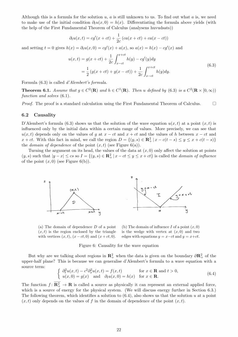
D’Alembert’s formula (6.3) shows us that the solution of the wave equation u(x, t) at a point (x, t) isinfluenced only by the initial data within a certain range of values. More precisely, we can see thatu(x, t) depends only on the values of g at x − ct and x + ct and the values of h between x − ct andx + ct. With this fact in mind, we call the region D = (y, s) ∈ R2

+ |x − c(t − s) ≤ y ≤ x + c(t − s)the domain of dependence of the point (x, t) (see Figure 6(a)).

Turning the argument on its head, the values of the data at (x, 0) only affect the solution at points(y, s) such that |y− x| ≤ cs so I = (y, s) ∈ R2

+ |x− ct ≤ y ≤ x+ ct is called the domain of influenceof the point (x, 0) (see Figure 6(b)).

(a) The domain of dependence D of a point(x, t) is the region enclosed by the trianglewith vertices (x, t), (x− ct, 0) and (x+ ct, 0).

(b) The domain of influence I of a point (x, 0)is the wedge with vertex at (x, 0) and twoedges with equations y = x−ct and y = x+ct.

Figure 6: Causality for the wave equation

But why are we talking about regions in R2+ when the data is given on the boundary ∂R2

+ of theupper-half plane? This is because we can generalise d’Alembert’s formula to a wave equation with asource term:

∂2t u(x, t)− c2∂2

xu(x, t) = f(x, t) for x ∈ R and t > 0,u(x, 0) = g(x) and ∂tu(x, 0) = h(x) for x ∈ R.

(6.4)

The function f : R2+ → R is called a source as physically it can represent an external applied force,

which is a source of energy for the physical system. (We will discuss energy further in Section 6.3.)The following theorem, which identifies a solution to (6.4), also shows us that the solution u at a point(x, t) only depends on the values of f in the domain of dependence of the point (x, t).

22

Theorem 6.2. Assume that g ∈ C2(R), h ∈ C1(R) and f ∈ C1(R2+). Then u defined by

u(x, t) =1

2(g(x+ ct) + g(x− ct)) +

1

2c

∫ x+ct

x−cth(y)dy +

1

2c

∫ t

0

∫ x+c(t−s)

x−c(t−s)f(y, s)dyds (6.5)

is a C2(R× [0,∞)) function and solves (6.4).

Proof. We recognise the first two terms in (6.5) from (6.3), so we know these two terms provide asolution to (6.1). Since the wave equation is linear, it only remains to check that the last term in (6.5)

v(x, t) =1

2c

∫ t

0

∫ x+c(t−s)

x−c(t−s)f(y, s)dyds

is a C2(R× [0,∞)) function and solves∂2t v(x, t)− c2∂2

xv(x, t) = f(x, t) for x ∈ R and t > 0,v(x, 0) = 0 and ∂tv(x, 0) = 0 for x ∈ R.

Clearly v(x, 0) = 0. We also have

∂tv(x, t) =1

2c

∫ x

xf(y, t)dy +

1

2c

∫ t

0cf(x+ c(t− s), s) + cf(x− c(t− s), s)ds

=1

2

∫ t

0f(x+ c(t− s), s) + f(x− c(t− s), s)ds,

so, in particular, ∂tv(x, 0) = 0. Furthermore

∂ttv(x, t) =1

2(f(x, t) + f(x, t)) +

c

2

∫ t

0∂1f(x+ c(t− s), s)− ∂1f(x− c(t− s), s)ds

= f(x, t) +c

2

∫ t

0∂1f(x+ c(t− s), s)− ∂1f(x− c(t− s), s)ds

and

∂xv(x, t) =1

2c

∫ t

0f(x+ c(t− s), s)− f(x− c(t− s), s)ds,

so

∂xxv(x, t) =1

2c

∫ t

0∂1f(x+ c(t− s), s)− ∂1f(x− c(t− s), s)ds.

Therefore

∂ttv(x, t)− c2∂xxv(x, t) = f(x, t) +c

2

∫ t

0∂1f(x+ c(t− s), s)− ∂1f(x− c(t− s), s)ds

− c

2

∫ t

0∂1f(x+ c(t− s), s)− ∂1f(x− c(t− s), s)ds

= f(x, t).

Finally, we see that both ∂ttv and ∂xxv are continuous and we can also compute

∂txv(x, t) = ∂xtv(x, t) =1

2

∫ t

0∂1f(x+ c(t− s), s) + ∂1f(x− c(t− s), s)ds,

which is continuous too, so v ∈ C2(R× [0,∞)).

23

6.3 Energy

Recall from (3.1) that c2 = T/ρ where T is tension and ρ is mass density. Adjusting our point ofview from the two dimensional motivation (n = 2) in Section 3.1 to that of one spatial dimension(n = 1) a reasonable physical situation to have in mind is that of a vibrating string. The mass densityρ is now mass per unit length of string and the tension T is the force acting tangent to the string. Asolution u(x, t) to the wave equation represents the vertical displacement the string at a given horizontalcoordinate x and time t. We know from physics that the energy associated with motion (kinetic energy)is given by half of the mass times velocity squared. Thus the kinetic energy per unit length at positionx and time t is given by 1

2ρ(∂tu(x, t))2, and so the kinetic energy of the whole string is

1

2

∫ ∞−∞

ρ(∂tu(x, t))2dx.

The elastic energy stored in the string by virtue of its shape (potential energy) is given by the de-formation times the force exerted while performing that deformation. The force acting as the stringstretches and contracts will be T and thus constant. The length of the string at a given time t is givenby the length of the graph of x 7→ u(x, t), which is∫ ∞

−∞

√1 + (∂xu(x, t))2dx.

Thus the change in the length of the string, compared to when it is not deformed at all (u(x, t) = 0) is∫ ∞−∞

(√1 + (∂xu(x, t))2 − 1

)dx ≈ 1

2

∫ ∞−∞

(∂xu(x, t))2dx,

and so we take the potential energy to be

1

2

∫ ∞−∞

T (∂xu(x, t))2dx.

We define the energy of u at time t to be the sum of the kinetic and potential energy:

E[u](t) :=1

2

∫ ∞−∞

ρ(∂tu(x, t))2 + T (∂xu(x, t))2dx. (6.6)

Although energy will be transformed from kinetic to potential and back again as the string vibrates,we would expect the total energy to be conserved. This is the content of the next theorem.

Theorem 6.3. Assume that u ∈ C2(R × [0,∞)) solves ∂ttu(x, t) − c2∂xxu(x, t) = 0 (with c2 = T/ρ),is such that ∂tu(x, t)→ 0 and ∂xu(x, t)→ 0 as x→ ±∞, and the integrals∫ ∞

−∞|∂αu(x, t)|2dx

converge uniformly in t, where ∂α is any derivative of order less than or equal to two.5 Then E[u]defined in (6.6) is a constant function.

Proof. Differentiating the kinetic energy and using the wave equation u solves, we have

d

dt

(1

2

∫ ∞−∞

ρ(∂tu(x, t))2dx

)=

1

2

∫ ∞−∞

ρ∂tu(x, t)∂ttu(x, t)dx

=1

2

∫ ∞−∞

T∂tu(x, t)∂xxu(x, t)dx = −1

2

∫ ∞−∞

T∂txu(x, t)∂xu(x, t)dx

= − d

dt

(1

2

∫ ∞−∞

T (∂xu(x, t))2dx

).

5For those who are familiar with the notation, α is a multi-index with order |α| ≤ 2.

24

Therefored

dt

(1

2

∫ ∞−∞

ρ(∂tu(x, t))2 + T (∂xu(x, t))2dx

)= 0

and the theorem is proved.

Remark 6.4. We can modify the defintion of energy by a multiplicative factor and we would still havea conserved quantity. Indeed if we modified the definition by dividing by ρ, the energy would be

1

2

∫ ∞−∞

(∂tu(x, t))2 + c2(∂xu(x, t))2dx

which is an expression which only involves constants (namely c) which directly appear in the waveequation. However, the definition we have taken is consistent with that used in physics.

Corollary 6.5. (a) For any given functions g and h, there is at most one solution u to (6.1) whichsatisfies the same hypothesis as in Theorem 6.3.

(b) For any given functions g, h and f , there is at most one solution u to (6.4) which satisfies thesame hypothesis as in Theorem 6.3.

Proof. In both cases the difference of two solutions w = u1−u2 solves (6.1) with g = h = 0. Therefore,by Theorem 6.3,

1

2

∫ ∞−∞

ρ(∂tw(x, t))2 + T (∂xw(x, t))2dx = E[w](t) = E[w](0) = 0.

In particular this implies ∂tw(x, t) = 0, so w(x, t) is a function of x only and in particular w(x, t) =w(x, 0). But this function must be zero, since w(x, 0) = 0.

6.4 Reflections

6.4.1 Waves on the half-line

So far we have only considered the wave equation on the real line, which would model the motion ofa vibrating string which is infinitely long. This is perhaps slightly unrealistic, as we are much morelikely to encounter strings of finite length in the real world. In this section we will consider a situationwhich could be described as half-way between an infinitely long string and a finite length string. InSection 6.4.2 we will extend the method used here to deal with the finite case.

We will consider the wave equation on the positive half-line with a Dirichlet boundary condition.Given g, h : [0,∞)→ R we wish to find v : [0,∞)× [0,∞)→ R such that

∂ttv(x, t)− c2∂xxv(x, t) = 0 for x ∈ (0,∞) and t > 0,v(x, 0) = g(x) and ∂tv(x, 0) = h(x) for x ∈ [0,∞), andv(0, t) = 0 for t > 0.

(6.7)

We can relate (6.7) to the analogous problem (6.1) on the whole real line. Suppose u solved (6.1)with initial values godd and hodd, the odd extensions of g and h:

godd(x) :=

g(x) if x ≥ 0, and−g(−x) if x < 0;

and

hodd(x) :=

h(x) if x ≥ 0, and−h(−x) if x < 0.

Homework exercise 5.2 shows that

u(x, t) =1

2(godd(x+ ct) + godd(x− ct)) +

1

2c

∫ x+ct

x−cthodd(y)dy (6.8)

25

would be an odd function for each t > 0. Thus, in particular u(0, t) = 0 for all t > 0, and v(x, 0) = g(x)and ∂tv(x, 0) = h(x) for all x ∈ [0,∞), so u restricted to x ≥ 0 is the solution to (6.7) we are lookingfor.

Observe that if (6.8) is to be a solution to (6.1) then according to Theorem 6.1 we need to knowthat godd ∈ C2(R) and hodd ∈ C1(R). This will only be the case if g ∈ C2([0,∞)) and h ∈ C1([0,∞))and g(0) = h(0) = 0.

We formulate the preceeding discussion as a theorem.

Theorem 6.6. Suppose g ∈ C2([0,∞)), h ∈ C1([0,∞)) and g(0) = h(0) = 0. Then the functionv : [0,∞)× [0,∞)→ R defined by

v(x, t) =1

2(godd(x+ ct) + godd(x− ct)) +

1

2c

∫ x+ct

x−cthodd(y)dy.

for x ≥ 0 and t ≥ 0 is a C2([0,∞)× [0,∞)) function which solves (6.7).

6.4.2 Waves on a finite interval

Now consider the wave equation on a finite interval [0, `] with Dirichlet boundary conditions. Giveng, h : [0, `]→ R we wish to find v : [0, `]× [0,∞)→ R such that

∂ttv(x, t)− c2∂xxv(x, t) = 0 for x ∈ (0, `) and t > 0,v(x, 0) = g(x) and ∂tv(x, 0) = h(x) for x ∈ [0, `], andv(0, t) = 0 and v(`, t) = 0 for t > 0.

(6.9)

Once again, we can relate (6.9) to the analogous problem (6.1) on the whole real line. Suppose usolved (6.1) with initial values gext and hext, the following extensions of g and h:

gext(x) :=

g(x− 2`n) if x ∈ [2`n, 2`n+ `] for some n ∈ Z,−g(−x+ 2`n) if x ∈ (2`n− `, 2`n) for some n ∈ Z;

so gext is an odd extension of g with respect to both x = 0 and x = ` (and also 2`-periodic), and

hext(x) :=

h(x− 2`n) if x ∈ [2`n, 2`n+ `] for some n ∈ Z,−h(−x+ 2`n) if x ∈ (2`n− `, 2`n) for some n ∈ Z;

so hext is also an odd extension of h with respect to both x = 0 and x = ` (and 2`-periodic).Homework exercise 5.2 and the translation invariance of the wave equation proved in exercise 5.5a

shows that

u(x, t) =1

2(gext(x+ ct) + gext(x− ct)) +

1

2c

∫ x+ct

x−cthext(y)dy

would be an odd function with respect to both x = 0 and x = ` for each t > 0. Thus, in particularu(0, t) = 0 and u(`, t) = 0 for all t > 0, and v(x, 0) = g(x) and ∂tv(x, 0) = h(x) for all x ∈ [0, `], so urestricted to 0 ≤ x ≤ ` is the solution to (6.9) we are looking for.

We must also once again impose conditions on g and h that ensure gext and hext are suitable smooth.All these considerations give us the following theorem.

Theorem 6.7. Suppose g ∈ C2([0, `]), h ∈ C1([0, `]) and g(0) = h(0) = g(`) = h(`) = 0. Then thefunction v : [0,∞)× [0,∞)→ R defined by

v(x, t) =1

2(gext(x+ ct) + gext(x− ct)) +

1

2c

∫ x+ct

x−cthext(y)dy.

for 0 ≤ x ≤ ` and t ≥ 0 is a C2([0, `]× [0,∞)) function which solves (6.9).

26

6.5 Higher dimensions

6.5.1 Three spatial dimensions: spherical means

In this section we will derive a formula for solutions u : R3 × [0,∞)→ R to the wave equation

∂ttu(x, y, z, t)− (∂xx + ∂yy + ∂zz)u(x, y, z, t) = 0 for t > 0 and (x, y, z) = x ∈ R3 (6.10)

(where for simplicity we set c = 1) with the initial conditions

u(x, 0) = φ(x), and ∂tu(x, 0) = ψ(x) for x ∈ R3.

This will be achieved by studying the properties of spherical means ux of u about a fixed x ∈ R3

defined to be

ux(r, t) =1

4πr2

∫|y−x|=r

u(y, t)dσ(y) for t, r > 0.

We begin by applying the Divergence Theorem to a solution u to (6.10) in the ball Br(x) = y ∈Rn | |y − x| < r:∫∫∫

Br(x)∂ttu(y, t)dy =

∫∫∫Br(x)

∇u(y, t)dy =

∫∫∂Br(x)

n · ∇u(y, t)dσ(y) (6.11)

which can be rewritten in polar coordinates as∫ r

0

∫ 2π

0

∫ π

0(∂ttu)ρ2 sin θdθdφdr =

∫ 2π

0

∫ π

0(∂ru)r2 sin θdθdφ

and simplified to ∫ r

0ρ2∂ttux(ρ, t)dr = r2∂rux(r, t).

Differentiating with respect to r gives

r2∂ttux(r, t) = r2∂rrux(r, t) + 2r∂rux(r, t). (6.12)

With the substitution v(r, t) = rux(r, t) we have ∂ttv(r, t) = r∂ttux(r, t) and ∂rrv(r, t) = r∂rrux(r, t) +2∂rux(r, t) so that, dividing (6.12) by r, we obtain

∂ttv(r, t) = ∂rrv(r, t) for r, t > 0. (6.13)

Moreover v(0, t) = 0×u(0, t) = 0, so v satisfies (6.7) for some g and h. We now wish to make use (6.8),so we must calculate the initial values g and h appearing in (6.7). Clearly

v(r, 0) = rφx(r) and ∂tv(r, 0) = rψx(r),

with

φx(r) :=1

4πr2

∫|y−x|=r

φ(y)dσ(y) and ψx(r) :=1

4πr2

∫|y−x|=r

ψ(y)dσ(y).

Therefore rewriting (6.8) for the present case gives that

v(r, t) =∂

∂t

(1

2

∫ r+t

t−rsφx(s)ds

)+

1

2

∫ r+t

t−rsψx(s)ds

at least in the case 0 ≤ r ≤ t.We can now recover u(x, t) as

u(x, t) = limr→0

ux(r, t) = limr→0

v(r, t)

r= lim

r→0

v(r, t)− v(0, t)

r= ∂rv(0, t).

27

We calculate

∂rv(r, t) =∂

∂t

(1

2

((r + t)φx(r + t) + (t− r)φx(t− r)

))+

1

2

((r + t)ψx(r + t) + (t− r)ψx(t− r)

)so

u(x, t) =∂

∂t

(tφx(t)

)+ tψx(t) =

∂

∂t

(1

4πt

∫|y−x|=t

φ(y)dσ(y)

)+

1

4πt

∫|y−x|=t

ψ(y)dσ(y). (6.14)

Thus we have derived a formula for a solution to the wave equation (6.10) in three spatial dimensionsby relating it to a similar problem for the wave equation (6.7) in one spatial dimension. This formula(6.14) is called Kirchoff’s formula.

Observe that the solution u(x, t) only depends on the initial data at values y lying in the sphere|y − x| = t. This is called Huygen’s Principle. A consequence of this is that the sound transmitted bya speaker in three dimensional space sound to a listener regardless of the distance between the speakerand listener. As we have seen, this is not the case in one dimensional space. Indeed, in one dimensiond’Alemberts formula (6.3) (say with c = 1) shows that the solution depends not just on the the data adistance t from the listener, but all distances up to t. Thus sound transmitted by a speaker will sounddifferent depending on the distance between the speaker and the listener. In Section 6.5.2 we will seethis is also the case in two dimensions. In general Huygen’s Principle holds in odd dimensions greaterthan one and does not in even dimensions.

6.5.2 Two spatial dimensions: the method of descent

With the help of Kirchoff’s formula (6.14) in three spatial dimensions it is easy to derive a formula forthe solution to the initial value problem

∂ttv(x, y, t)− (∂xx + ∂yy)v(x, y, t) = 0 for (x, y) ∈ R2 and t > 0,v(x, y, 0) = φ(x, y) and ∂tv(x, y, 0) = ψ(x, y) for (x, y) ∈ R2.

(6.15)

We do this by viewing a solution to (6.15) as a solution to (6.10) which happens to be constant in thez-direction. Kirchoff’s formula (6.14) says

u(x, y, t) =∂

∂t

(1

4πt

∫(x−a)2+(y−b)2+(z−c)2=t2

φ(a, b)dσ(a, b, c)

)

+1

4πt

∫(x−a)2+(y−b)2+(z−c)2=t2

ψ(a, b)dσ(a, b, c)

=∂

∂t

(1

2πt

∫(x−a)2+(y−b)2≤t2

φ(a, b)

)+

1

2πt

∫(x−a)2+(y−b)2≤t2

ψ(a, b)dadb.

and parametrising the sphere (x − a)2 + (y − b)2 + (z − c)2 = t2 in the variables a and b with twohemispheres c = ±

√t2 − a2 − b2 we find that

dσ(a, b, c) =

√1 +

(∂c

∂a

)2

+

(∂c

∂b

)2

dadb =

√((t2 − a2 − b2) + a2 + b2) dadb

t2 − a2 − b2=

tdadb√t2 − a2 − b2

so

u(x, y, t) =∂

∂t

(1

2π

∫(x−a)2+(y−b)2≤t2

φ(a, b)√t2 − a2 − b2

dadb

)

+1

2π

∫(x−a)2+(y−b)2≤t2

φ(a, b)√t2 − a2 − b2

dadb.

(6.16)

This formula proves the claim we made in Section 6.5.1 that Huygen’s Principle does not hold in twodimensions. The solution u(x, y, t) from (6.16) depends on the data in a disc of radius t about (x, y),not just on the circle of radius t centred at (x, y).6

6A sphere and ball in two dimensions are usually called a circle and disc, respectively.

28

7 The heat equation

We now move on to study another PDE that appeared in Section 3, namely the heat equation (Section3.2). For simplicity we will take the proportionality constant k that appeared there to be equal toone. We will pose similar questions to those we asked regarding Laplace’s equation and the waveequation, but we will see that the answers demonstrate there are differences between the PDEs as wellas similarities.

7.1 Another maximum principle

In this section we will consider solutions u : Ω×[0, T ]→ R to the heat equation ∂tu(x, t)−∆u(x, t) = 0,where Ω ⊂ Rn is an open bounded connected set and T > 0. We begin with a property that is verysimilar to one exhibited by harmonic functions. It’s proof is also similar to the case of harmonicfunctions, but we repeat it in detail here for completeness.

Theorem 7.1 (Weak Maximum Principle). Suppose Ω ⊂ Rn is an open bounded connected set andT > 0. Let u : Ω × [0, T ] → R be a continuous function which is also a solution to the heat equation∂tu(x, t) − ∆u(x, t) = 0 for (x, t) ∈ Ω × (0, T ]. Then the maximum value of u is attained at a point(x, t) ∈ Ω× [0, T ] such that either t = 0 or x ∈ ∂Ω.

Remark 7.2. Theorem 7.1 says that the maximum of u is either obtained initially (t = 0) or on thelateral edges of the domain (x ∈ ∂Ω).

Theorem 7.1 does not rule out the possibility that the maximum is also obtained in Ω × (0, T ]. Itturns out, however, that one can rule out such a possibility, although the proof is much more difficult,so we will not do this here.

Just as for Theorem 5.1, we can make an analogous statement about the minimum of u.

Proof of Theorem 7.1. For ε > 0 set v(x, t) = u(x, t) + ε|x|2. Since v is continuous on the compact setΩ× [0, T ] it must attain a maximum somewhere in Ω× [0, T ].

Suppose v attains this maximum at (x, t) with x ∈ Ω and 0 < t ≤ T , then, by the first derivativetest, ∂tu(x, t) = 0 and by the second derivative test, ∆v(x) =

∑nj=1 ∂

2j v(x) ≤ 0. This means

∂tv(x, t)−∆v(x, t) ≥ 0− 0 = 0.

On the other hand, since u solves the heat equation, we can compute

∂tv(x, t)−∆v(x, t) = ∂tu(x, t)−∆u(x, t)− 2nε = 0− 2nε < 0,

which is a contradiction.Therefore v must attain its maximum at a point (x, t) for which either x ∈ ∂Ω or t = 0. Set

M = max(x,t)∈B u(x, t) where B = (Ω× 0) ∪ (∂Ω× (0, T ]), then

maxΩ×[0,T ]

u ≤ maxΩ×[0,T ]

v ≤ maxB

v ≤ maxB

u+ εD = M + εD.

Since ε is arbitrary we must have maxΩ×[0,T ] u ≤M .

Theorem 7.1 can be used to prove the uniqueness of solutions to initial boundary value problemsfor the heat equation (see homework exercise 6.2(b)), however we will use the energy method below toprove the same result.

7.2 Uniqueness and stability via the energy method

Consider the initial boundary value problem∂tu(x, t)−∆u(x, t) = 0 for x ∈ Ω and t ∈ (0, T ];

u(x, 0) = φ(x) for x ∈ Ω; andu(y, t) = g(y, t) for y ∈ ∂Ω and t ∈ (0, T ].

(7.1)

29

One can show that if g = 0, the quantity ∫Ω|u(x, t)|2dx

is a decreasing function of t. Indeed, suppose u ∈ C1(Ω× [0, T ]) and is also a solution to (7.1). Thenusing (5.8)

d

dt

∫Ω|u(x, t)|2dx =

∫Ωu(x, t)∂tu(x, t)dx

=

∫Ωu(x, t)∆u(x, t)dx = −

∫Ω∇u(x, t)∇u(x, t)dx = −

∫Ω|∇u(x, t)|2dx ≤ 0.

In particular, we have

0 ≤∫Rn

|u(x, t)|2dx ≤∫Rn

|φ(x)|2dx

for all t ∈ [0, T ]. This means that if we had two solutions u1 and u2 of (7.1), then their differencew = u2 − u2 would satsify (7.1) with φ = 0 and g = 0, so

0 ≤∫Rn

|u2(x, t)− u1(x, t)|2dx =

∫Rn

|w(x, t)|2dx ≤ 0.

Whence u1 = u2. This proves the following theorm.

Theorem 7.3. There is at most one function u ∈ C1(Ω× [0, T ]) which is also a solution to (7.1).

The same method also tells us the solution depends continuously on the data. Recall this was thethird criteria, which we called stability, required in Section 4.4 for a problem to be well-posed.

Theorem 7.4. Suppose ui ∈ C1(Ω× [0, T ]) solves (7.1) with g = gi and φ = φi for i = 1, 2. If g1 = g2,then

0 ≤∫

Ω|u2(x, t)− u1(x, t)|2dx ≤

∫Ω|φ2(x)− φ1(x)|2dx

A similar, but different, stability (homework exercise 6.2(c)) can be proved for the heat equationusing the Weak Maximum Principle (Theorem 7.1).

7.3 The initial value problem on the real line

Now consider the initial value problem∂tu(x, t)− ∂xxu(x, t) = 0 for x ∈ R and t ∈ (0,∞);u(x, 0) = φ(x) for x ∈ R.

(7.2)

In this section we will show that it is possible to find a solution to such a problem. To do this thefunction S : R× (0,∞)→ R defined by

S(x, t) =1

2√πte−x

2/4t

will be extremely important to us. This function is called the heat kernel. In Chapter 2.4 of Strauss ajustification for studying this particular function is given.

Observe that

∂tS(x, t) =−1

4√πt3/2

e−x2/4t +

x2

8√πt5/2

e−x2/4t

and∂xS(x, t) = − x

4√πt3/2

e−x2/4t

30

so

∂xxS(x, t) = − 1

4√πt3/2

e−x2/4t +

x2

8√πt5/2

e−x2/4t.

This implies ∂tS(x, t)− ∂xxS(x, t) = 0, that is, S solves the heat equation.For each t > 0 the function x 7→ S(x, t) is a Gaussian. You may have encountered such a function

before in perhaps Calculus (as a function we can integrate on the real line without calculating aprimative function) or probability theory (normal distributions). Observe that for small t the graph ofx 7→ S(x, t) has a tall thin spike around zero and decays rapidly to zero as |x| increases. For large t,the graph of x 7→ S(x, t) is fattened out, so that the spike at zero is more like a gentle hill. Considerthe integral

u(x, t) =

∫ ∞−∞

S(x− y, t)φ(y)dy. (7.3)

If t is small, the integral in (7.3) would average φ over a very small interval near x. If we let t → 0we might expect these averages of φ near x to converge to φ(x). Moreover, because S solves the heatequation and the heat equation is translation invariant (that is, (x, t) 7→ S(x − y, t) is also a solutionfor each y ∈ R) we expect (7.3) to also be a solution to the wave equation, as it is essentially a linearcombination of solutions. This means, that we would guess that (7.3) would be a solution to (7.2).This guess is in fact correct, as the following proof shows.

Theorem 7.5. Let φ : R → R be a bounded continuous function. Then (7.3) defines an infinitelydifferentiable function on the set R2

+ := (x, t) |x ∈ R, t > 0, which satisfies ∂tu(x, t)− ∂xxu(x, t) = 0for (x, t) ∈ R2

+ and limt→0+ u(x, t) = φ(x) for each x ∈ R.

Proof. First we perform a change of variables

u(x, t) =

∫ ∞−∞

S(x− y, t)φ(y)dy =

∫ ∞−∞

S(z, t)φ(x− z)dz =

∫ ∞−∞

S(p√t, t)φ(x− p

√t)√tdp.

Then it is easy to see that S(p√t, t)φ(p

√t− x)

√t = e−p

2/4

2√πφ(p√t− x). This means that the integrand

is bounded above by 12√π

supy∈R |φ(y)|e−p2/4, so the integral in p above converges uniformly in x andt.

Moreover, u(x, t) will be differentiable any number of times with respect to x or t, say α times,where α is a multi-index, and equal to

∂αu(x, t) =

∫ ∞−∞

∂αS(x− y, t)φ(y)dy

provided we can justify interchanging differentiation and integration. To justify this is suffices to showthe integrand above is uniformly integrable. This can be done just as before, since differentiating Sjust introduces a polynomial in p in front of e−p

2/4 (together with factors of t). This polynomial growthis not enough to destroy the uniform convergence of the integral due to the exponential decay e−p

2/4.For example,∫ ∞

−∞∂1S(x− y, t)φ(y)dy =

∫ ∞−∞

∂1S(z, t)φ(z − x)dz =

∫ ∞−∞

∂1S(p√t, t)φ(p

√t− x)

√tdp.

Since ∂1S(x, t) = − x4√πt3/2

e−x2/4t, we have that ∂1S(p

√t, t)φ(p

√t − x)

√t = −pe−p

2/4

4√πt

φ(p√t − x) so,

because |∂1S(p√t, t)φ(p

√t − x)

√t| ≤ pe−p

2/4

4√πt

supy∈R |φ(y)|, we see that ∂1S(p√t, t)φ(p

√t − x)

√t is

integrable in p uniformly in x and t.Now we know that we can justify interchanging differentiation and integration, it follows from the

fact that S solves the heat equation, that (7.3) also solves the heat equation.It remains to prove the initial condition holds. We can calculate that∫ ∞

−∞S(x, t)dx = 1.

31

Therefore

u(x, t)− φ(x) =

∫ ∞−∞

S(x− y, t)(φ(y)− φ(x))dy =

∫ ∞−∞

S(p√t, t)(φ(p

√t− x)− φ(x))

√tdp

=

∫ ∞−∞

1

2√πe−p

2/4(φ(p√t− x)− φ(x))dp.

The idea of the proof from here is to split the integral in two. The integral over p close to the originwill be small because |φ(p

√t − x) − φ(x)| will be small if t is small. Recalling that the graph of

p 7→ 12√πe−p

2/4 will look like a bump centred at the origin and decay quickly away from the origin, the

integral over large p will be also be small.Fix ε > 0. We choose δ > 0 so small that

max|y−x|≤δ

|φ(y)− φ(x)| < ε/2

Then we rewrite the integral as∫ ∞−∞

1

2√πe−p

2/4(φ(p√t− x)− φ(x))dp

=

∫|p|<δ/

√t

1

2√πe−p

2/4(φ(p√t− x)− φ(x))dp+

∫|p|≥δ/

√t

1

2√πe−p

2/4(φ(p√t− x)− φ(x))dp

We can bound the first integral using our choice of δ:∣∣∣∣∣∫|p|<δ/

√t

1

2√πe−p

2/4(φ(p√t− x)− φ(x))dp

∣∣∣∣∣ ≤ ε

2

∫|p|<δ/

√t

1

2√πe−p

2/4dp ≤ ε

2,

since∫|p|<δ/

√t

12√πe−p

2/4dp ≤∫∞−∞

12√πe−p

2/4dp = 1. The first integral can also be bounded using the

boundedness of φ. If we take C to be the constant such that |φ(x)| ≤ C for all x ∈ R (which existssince φ is bounded), then∣∣∣∣∣

∫|p|≥δ/

√t

1

2√πe−p

2/4(φ(p√t− x)− φ(x))dp

∣∣∣∣∣ ≤ 2C

∫|p|≥δ/

√t

1

2√πe−p

2/4dp.

We can make the last integral less than ε/2 since the last integral is just the ‘tails’ of a convergentintegral, so will small for sufficiently small t. Thus we have proved u(x, t)→ φ(x) as t→ 0.

7.4 A comparison of the wave and heat equations

We saw in Section 6.2 that the wave equation transmitted information at speed at most c. The datathat affected the solution at a given point (x, t) depended only on the data within the domain ofdependence of (x, t). This made sense given the physical motivation for studying the equation.

At first sight it would be reasonable to expect the same of the heat equation. Heat can surely onlyflow from one place to another at a finite speed. However, a closer look at formula (7.3) shows this isnot the case.

Consider (7.2) with data φ given by

φ(x) =

1− |x| for |x| < 1;0 for |x| ≥ 1.

Formula (7.3) gives a solution to (7.2). Since S is positive it is clear that the solution u(x, t) will alsobe positive for all x ∈ R and t > 0. Physically this says that the initial heat, which was localised to|x| < 1, has travelled an arbitrarily large distance in an arbitrarily small time. Consequently we do nothave the finite speed of propagation we saw for wave equation in the heat equation.

Theorem 7.5 shows that with just bounded and continuous data φ the solution to the heat equation(7.2) will be infinitely differentiable for t > 0. This is clearly not the case for the wave equation, aswe can see from D’Alemberts formula (6.3). Thus it is reasonable to say that the heat equation issmoothing, but the wave equation is not.

In Table 1 we compare the properties of solutions to the two equations.

32

Property Wave equation Heat equation

Speed of propogation Finite InfiniteSmoothing No YesSupports a maximum principle No YesEnergy Conserved DecaysTime reversable Yes No

Table 1: Properties of the wave and heat equations.

7.5 The heat equation on a bounded interval

We will conclude our investigation of the heat equation by considering solutions defined on a boundedinterval. More precisely, we want to find u : [0, `]× [0,∞)→ R such that

∂tu(x, t)− ∂xxu(x, t) = 0 for x ∈ (0, `) and t ∈ (0,∞);u(x, 0) = φ(x) for x ∈ [0, `];u(0, t) = 0 and u(`, t) = 0 for t > 0.

(7.4)

When we considered a similar domain for the wave equation we used ideas about reflection in order toconstruct a solution. Such a method would work well here, but we will try another method, separationof variables, which we have already applied to Laplace’s equation.

Suppose that a solution to (7.4) can be written in the form

u(x, t) = X(x)T (t).

Substututing this into the heat equation, we see that

X(x)T ′(t)−X ′′(x)T (t) = 0

so, dividing by X(x)T (t), we see thatT ′(t)

T (t)=X ′′(x)

X(x)

which must be independent of x and t, so equal to −λ, say. This gives us two ODEs to solve, the firstis

X ′′(x) + λX(x) = 0 for x ∈ [0, `], and X(0) = 0 and X(`) = 0 (7.5)

so a calculation shows that we must have λ = (kπ/`)2 and X(x) = A sin(kπx/`) for a constant A andk ∈ N. The second equation is

T ′(t) + λT (t) = 0 for t > 0

and a calculation shows that we must have T (t) = Be−λt = Be−(kπ/`)2t for a constant B and k ∈ N.We can take linear combinations of such solutions and so we find

u(x, t) =∞∑k=1

Ake−(kπ/`)2t sin(kπx/`). (7.6)

If such a sum is convergent, it will solve the heat equation and the boundary conditions u(0, t) =u(`, t) = 0. To ensure the initial condition is satisfied, we require

φ(x) =

∞∑k=1

Ak sin(kπx/`).

Thus we require that φ can be expressed as a Fourier sine series. This is certainly possible if φ isdifferentiable (although we will not prove this here). In this case, the coefficients are given by

Ak =2

`

∫ `

0φ(x) sin(kπx/`)dx.

33

8 Numerical analysis

In the preceding sections we have computed explicit formulae for solutions to PDEs in several particularsituations. However, in many situations it is not always possible to find such explicit formulae or, evenwhen it is possible, they may prove to be so complicated that they are not practical to use.

The aim of this section is to come up with a scheme that will produce an approximate solutionto a PDE together with its boundary/initial conditions by carrying out a finite number of arithmeticoperations. Such a scheme could then be implemented by a computer.

Care must be taking when devising such a scheme. We will have to check that any proposed schemedoes indeed approximate the solution we are looking for. Below we will see an example of what at firstappears to be a reasonable scheme that produces an ‘approximation’ which is very far from the truesolution.

Here we will illustrate the most important methods and techniques using simple equations asexamples.

8.1 Finite differences

The notion of a limit is central to the notion of a derivative. However, we cannot compute a limitin a finite number of arithmetic operations, so we must find a suitable replacement. One naturallypossibility is that of finite differences.

Consider a function u : R → R of one variable. We first choose a collection of points xj from thefunctions domain R. We can do this by first choosing a mesh size δx and then defining xj = j(δx).We can then denote

uj = u(xj).

We have three standard approximations for the first derivative u′(xj).

The backward difference:uj − uj−1

δx.

The forward difference:uj+1 − uj

δx.

The centred difference:uj+1 − uj−1

2δx.

They are approximations in the sense that the difference between them and the true value of u′(xj) issmaller the smaller δx is. This can be proved using the Taylor expansion for u. If u ∈ C4(R) then

u(x+ h) = u(x) + u′(x)h+u′′(x)

2h2 +

u′′′(x)

6h3 +O(h4). (8.1)

Taking x = xj and h = −δx we see that

u′(xj) =uj − uj−1

δx+O(δx),

taking x = xj and h = δx we see

u′(xj) =uj+1 − uj

δx+O(δx),

and finally taking the difference of (8.1) with x = xj and h = δx, and x = xj and h = −δx we see that

u′(xj) =uj+1 − uj−2

2(δx)+O((δx)2).

Adding the same two expressions from (8.1) gives us

u′′(xj) =uj+1 − 2uj + uj−1

(δx)2+O((δx)2),

34

which motivates the following approximation for the second derivative u′′(xj):

The centred second difference:uj+1 − 2uj + uj−1

(δx)2.

We will of course be interested in functions of more than one variable. In particular if we have afunction u of two variables x and t, we choose mesh sizes δx and δt for each variable. We write

u(j(δx), n(δt)) = unj .

Then we can approximate ∂tu(j(δx), n(δt)) by, for example, the forward difference

un+1j − unjδt

.

Similarly, the forward difference for ∂xu(j(δx), n(δt)) is

unj+1 − unjδx

,

and so on.

8.2 Approximating solutions to the heat equation

8.2.1 An unstable scheme

We begin with what appears to be a simple problem. Let’s use the above approximations to producea scheme for finding approximate solutions to (7.4), the heat equation on a bounded domain with theinitial condition u(x, 0) = φ(x). We can use a forward difference to approximate ut and a centreddifference to approximate uxx. Then the PDE is replaced by the difference equation

un+1j − unjδt

=unj+1 − 2unj + unj−1

(δx)2. (8.2)

Choose a small value of δx so that xjJj=0 is a mesh over the interval [0, `] with xj = j(δx) and such

that xJ = ` and set δt = (δx)2. The equation becomes

un+1j − unj = unj+1 − 2unj + unj−1

soun+1j = unj+1 − unj + unj−1. (8.3)

Now the initial data provides the values u0j for all j = 0, 1, . . . , J , since we can impose that u0

j = φ(xj).Furthermore, the boundary conditions lead us to set un0 = unJ = 0 for all n = 1, 2, . . . . Then (8.3) canbe used to obtain first u1

j for all j, then u2j for all j and inductively all unj for all j and n.

Let’s implement this scheme with some simple initial data. For example, let’s suppose ` = 4,δx = 0.5 and u0

4 = φ(2) = 1 and u0j = φ(xj) = 0 for j 6= 4. Then we can compute the values unj as in

Table 2.Take a look at Table 2. Does anything appear to have gone wrong? Observe that |φ(x)| ≤ 1 for

all x but we have computed u50 = −51. If we compare the solution unj j,n of our numerical scheme

(8.3) to what Theorem 7.1 says about solutions to the heat equation, we see that our scheme has notproduced something close to the true solution.

In the next section we will investigate what has gone wrong and fix it to produce a much betterscheme.

35

j = 0 j = 1 j = 2 j = 3 j = 4 j = 5 j = 6 j = 7 j = 8

n = 0 0 0 0 0 1 0 0 0 0n = 1 0 0 0 1 -1 1 0 0 0n = 2 0 0 1 -2 3 -2 1 0 0n = 3 0 1 -3 6 -7 6 -3 1 0n = 4 0 -4 10 -16 19 -16 10 -4 0n = 5 0 14 -30 45 -51 45 -30 14 0

Table 2: Some values of unj computed via (8.3) together with the initial and boundary conditions.

8.2.2 A stability condition

We will now investigate why our scheme (8.3) failed. The problem is not easy to spot, although thereare subtle clues to what has gone wrong in the form of (8.3). Looking at Table 2, we see that thevalues of unj oscillate between positive and negative values; this property originates in the fact that

(8.3) contains negative coefficients. Let us return to our derivation of (8.3). Above we set δt = (δx)2

without much thought, but let’s repeat the calculation without this assumption. This time we set

s =δt

(δx)2.

Substituting this in (8.2) we obtain

un+1j = (unj+1 + unj−1)s+ (1− 2s)unj (8.4)

To investigate the stability of (8.4), let’s further investigate its solution. We can consider the scheme(8.4) together with the initial condition u0

j = φ(xj) for all j = 1, 2, . . . , J and boundary conditionsun0 = unJ = 0 for all n = 1, 2, . . . . It is not too hard to see that this determines unique values for all unjfor j = 1, 2, . . . , J and n = 1, 2, . . . . Let’s now show that these values can be decomposed as

unj = XjTn.

This anzats is the discrete form of separation of variables, that we employed in Section 7.5 for theactual heat equation. Given the method worked for the actual equation, there’s good reason to hopeit will work for the discrete approximation (8.2). Substituting this anzats in (8.4), we obtain

Tn+1

Tn= 1− 2s+ s

Xj+1 +Xj−1

Xj. (8.5)

We argue as usual that both sides must be a constant ξ independent of j and n. Therefore, Tn+1 = ξTnand so, by induction,

Tn = ξnT0.

At this point we can see that if our numerical approximation of a solution to the heat equation is notgoing to grow as n(δx) = t → ∞, which would contradict the maximum principle (see Theorem 7.1),then we require |ξ| ≤ 1. However, to determine what ξ is we must look at the right hand side of (8.5).

We have

sXj+1 +Xj−1

Xj+ 1− 2s = ξ. (8.6)

To find a solution of this, we guess that because when we solved the heat equation in Section 7.5 thecorresponding equation (7.5) was a second order ODE, this should be a discrete form of a second orderODE. Consequently, it is reasonable to guess solutions to (8.6) are of the form

Xj = A cos(jθ) +B sin(jθ),

for constants A, B and θ. The boundary condition un0 = 0 for all n = 1, 2, . . . implies A = 0 and we arefree to choose B = 1 as we can absorb any constant in Tn. The condition unJ = 0 for all n = 1, 2, . . .

36

implies sin(Jθ) = 0 and so Jθ = kπ for some fixed k ∈ N. But we know that J = `/δx, so θ = kπδx/`and

Xj = sin(jkπ(δx)/`).

Substituting this in (8.6) we have

ssin((j + 1)kπ(δx)/`) + sin((j − 1)kπ(δx)/`)

sin(jkπ(δx)/`)+ 1− 2s = ξ

which simplifies toξ = ξ(k) = 1− 2s(1− cos(kπ(δx)/`)). (8.7)

Thus, it is easy to see that 1− 4s ≤ |ξ| ≤ 1, so we can only guarantee that |ξ(k)| ≤ 1 if

δt

(δx)2= s ≤ 1

2. (8.8)

The condition (8.8) is a stability condition for the numerical scheme (8.4) — it ensures the values weobtain will not oscillate widely as in Section 8.2.1, but we have not said anything about how close ourapproximation is to the real solution.

However, we can give some justification that this is close to the true solution for small δx. Ourcalculations above show that the solution to the difference scheme (8.4) together with the boundaryconditions is

unj =

∞∑k=−∞

Bkξ(k)n sin(jkπ(δx)/`)

Comparing this to (7.6), we see that we need to justify that, for n(δt) = t fixed,

ξ(k)n → e−(kπ/`)2t

as δt→ 0 and n→∞. Expanding (8.7) as a Taylor series justifies the approximation

ξ(k) ≈ 1− s(

(kπ(δx)/`)2

2!

)= 1−

(kπ

`

)2

δt.

Raising this to the n-th power we have(1−

(kπ

`

)2

δt

)n=

(1−

(kπ

`

)2 nδt

n

)n=

(1−

(kπ

`

)2 t

n

)n≈ e−(kπ/`)2t,

as desired. Of course, this is far from a rigorous proof that our numerical scheme approximates thesolution, but it certainly provides some encouraging evidence.

8.2.3 The Crank-Nicolson Scheme

Although our choice of scheme (8.2) seemed quite natural, it was nevertheless somewhat arbitrary. Forexample, given that we used the forward difference (un+1

j − unj )/(δt) to approximate ut there is noparticular reason to use the centred difference

unj+1 − 2unj + unj−1

(δx)2

evaluated at time step n verses the centred difference

un+1j+1 − 2un+1

j + un+1j−1

(δx)2

37

evaluated at time step n+ 1 to approximate uxx. Indeed, here we will consider a mix of the two: for afixed θ ∈ [0, 1] we approximate uxx by

(1− θ)(unj+1 − 2unj + unj−1

(δx)2

)+ θ

(un+1j+1 − 2un+1

j + un+1j−1

(δx)2

)and then arrive at a replacement for (8.2)

un+1j − unjδt

= (1− θ)(unj+1 − 2unj + unj−1

(δx)2

)+ θ

(un+1j+1 − 2un+1

j + un+1j−1

(δx)2

)(8.9)

for approximating the heat equation. In the particular case θ = 0, (8.9) reduces to our old scheme(8.2), and in the case θ = 1/2, the scheme is called the Crank-Nicolson scheme. In contrast to (8.2) wecannot rewrite (8.9) as we did in (8.3), which gave un+1

j explicitly as an expression involving all the

earlier values (unj )j . Instead we obtain a system of linear equations for (un+1j )j in terms of the earlier

values (unj )j which must be solved. This is certainly a disadvantage, but let us now motivate why thescheme may be advantageous in another respect.

Analogously to (8.7), we can investigate the issue of stability by assuming a separated solution ofthe form

unj = eik(δx)jξ(k)n,

where, as before, k is chosen so that the solution automatically satisfies the zero boundary conditions.From this assumption we can calculate that

ξ(k) =1− (2− θ)s(1− cos(kδx)

1− 2θs(1− cos(kδx)

where s = δt/(δx)2 and we once again look to ensure |ξ(k)| ≤ 1 so that the solution does not grow forlarge n. It is easy to check that we always have ξ(k) ≤ 1 and the condition ξ(k) ≥ −1 requires

s(1− 2θ)(1− cos(kδx)) ≤ 1.

Since 1− cos(kδx) ≤ 2, this certainly holds if s(1− 2θ) ≤ 1/2, which is the case if either

1

2≤ θ ≤ 1 (8.10)

or

0 ≤ θ < 1

2and s ≤ 1

2(1− 2θ). (8.11)

Thus, at least from our preliminary calculations, it appears that (8.11) provides us with a stabilitycondition on s when θ < 1/2, but for θ ≥ 1/2, from (8.10) we conclude that the scheme (8.9) appearsto be stable regardless of the value of s.

8.3 Approximations of Laplace’s equation

8.3.1 A discrete mean value property

Let us now study Laplace’s equation in two dimensions. We begin just as before by defining grid pointsxj = j(δx) and yk = k(δy) for fixed δx and δy, and j, k ∈ Z. We can then approximate the Laplaceoperator ∆ = ∂xx + ∂yy by the sum of the centred differences. So, with uj,k = u(xj , yk), Laplace’sequation ∆u = 0 is approximated as

uj+1,k − 2uj,k + uj−1,k

(δx)2+uj,k+1 − 2uj,k + uj,k−1

(δy)2= 0.

If we choose δx = δy we can simplify this to

uj,k =1

4(uj+1,k + uj−1,k + uj,k+1 + uj,k−1) . (8.12)

38

Thus uj,k is the average of the values at the four adjacent points — that is, a discrete version of themean value property (Theorem 5.3) holds!7 Just as is the continuous case, we can use this to prove astrong maximum principle.

Given (j, k) ∈ Z2 we call (j + 1, k), (j − 1, k), (j, k + 1) and (j, k − 1) the adjacent points of (j, k).Given D ⊆ Z2, we say a point in D is an interior point of D if its adjacent points are also contained inD and a point is a boundary point if at least one of it’s adjacent points is not contained in D. The setof all boundary points of D is denoted ∂D. We say D ⊆ Z2 is discretely connected if, for each pair ofpoints p, q ∈ D, there exists N ∈ N and interior points pi for i = 1, . . . , N such that pi+1 is an adjacentpoint of pi for i = 0, . . . , N with p0 = p and pN+1 = q.

Theorem 8.1 (Discrete strong maximum principle). Suppose D ⊆ Z2 is discretely connected andu : D → R satisfies (8.12) (with u(j, k) = uj,k) at each interior point (j, k). Then, if u attains eithera maximum or minimum at an interior point of D, u is constant.

Again, just like the continuous case, this theorem can be used to prove the uniqueness of a solution(uj,k)j,k and in this case, the uniqueness of solutions also proves existence.

Theorem 8.2. Suppose D ⊆ Z2 is discretely connected and we are given an f : ∂D → R. Then thereexists a unique u : D → R that satisfies (8.12) (with u(j, k) = uj,k) at each interior point (j, k) andu(j, k) = f(j, k) for each (j, k) ∈ ∂D.

Proof. Suppose we have two functions v1, v2 : D → R satisfying the hypothesis of the theorem. Thenuj,k = v2(j, k) − v1(j, k) satisfies (8.12) at each interior point (j, k) and uj,k = 0 for each (j, k) ∈ ∂D.By Theorem 8.1 uj,k = 0 for all (j, k) ∈ D which implies v1 = v2 and we have proved uniqueness.

To prove existence, let N denote the number of interior points in D. Observe that (8.12) gives usN linear equations in the N unknowns uj,k, and this system can be written in the form Av = f , whereA is an N × N matrix, v is a vector with the N components uj,k, and f is a vector with elementsdepending on f such that f = 0 when f ≡ 0. By our proof of uniqueness above we have proved thatthe kernel of the matrix A is trivial. Therefore, by the rank-nullity theorem, the image of A is RN , sofor each f there exists a solution and we have proved existence.

8.3.2 The finite element method

So far in this chapter we have found numerical schemes to approximate the solution of differentialequations by replacing derivatives with finite differences. It seemed a natural approach, although, aswe saw, it also presented some problems. There are, however, other approaches that can also be taken.Once such alternative is called the finite element method. The method makes greater use of linearalgebra to approximate solutions.

We will study the Dirichlet problem for Poisson’s equation:−∆u = f in Ω, andu = 0 on ∂Ω.

(8.13)

First we shall find a convenient way to rewrite the boundary value problem. Let us denote the set of allfunctions v ∈ C2(Ω) which also satisfies the boundary condition v = 0 on ∂Ω by C2(Ω). If we multiplyboth side of the PDE in (8.13) by an arbitrary function v ∈ C2

0 (Ω), integrate over Ω and apply Green’sfirst identity (5.8), we obtain∫

Ω∇u(x) · ∇v(x)dx =

∫Ω

(−∆u)(x)v(x)dx =

∫Ωf(x)v(x)dx.

Interestingly, if we were given a function u ∈ C20 (Ω) such that∫

Ω∇u(x) · ∇v(x)dx =

∫Ωf(x)v(x)dx. (8.14)

7An equation involving finite differences is often refereed to as a discrete version, and its original form, involving eitherderivatives or integrals (and thus implicitly limits) is refereed to as the continuous version. Many ideas in calculus canbe formulated in both continuous and discrete versions. For example, summation by parts is the discrete analogue ofintegration by parts.

39

for all functions v ∈ C20 (Ω), then we could apply Green’s first identity again, to conclude∫

Ω(−∆u)(x)v(x)dx =

∫Ωf(x)v(x)dx.

Since v was arbitrary, from here we could conclude that −∆u = f . Thus, we see that if u ∈ C20 (Ω),

then (8.13) holds if and only if (8.14) holds for all v ∈ C20 (Ω). Observe that the boundary condition in

(8.13) holds by definition if u ∈ C20 (Ω).

The reformulation (8.14) is useful, as it emphasises the role of the vector space C20 (Ω). But how does

this help us find a numerical solution to (8.13)? The idea is to replace C20 (Ω) with a finite dimensional

vector subspace V of C20 (Ω). The task then becomes to uV ∈ V such that∫

Ω∇uV (x) · ∇v(x)dx =

∫Ωf(x)v(x)dx (8.15)

holds for all v ∈ V . If v1, v2, . . . , vN is a basis for V , then we can write

uV =N∑i=1

αivi,

N∑i=1

αi

∫Ω∇vi(x) · ∇vj(x)dx =

∫Ωf(x)vj(x)dx

for each j = 1, 2, . . . , N . Writing fk =∫

Ω f(x)vk(x)dx and mij =∫

Ω∇vi(x) · ∇vj(x)dx, this is just thesystem of linear equations,

N∑i=1

mijαi = fj ,

which can be easily solved by inverting the matrix (mij)ij .

Figure 7: A triangulation of the set Ω with interior vertices labelled x1,x2,x3,x4,x5.

In order to implement these ideas we need to find an explicit finite dimensional vector space V andassociated basis. One way to do this is to find a triangulation of Ω. This involves approximating Ωby a union of triangles (see Figure 7). Enumerate the vertices of the triangulation which lie in theinterior of Ω by x1,x2, . . . ,xN and then, for each k = 1, 2, . . . , N , define a function vk which is equalto one at xk, equal to zero at all other vertices, and extended to be linear in each triangle. Thus,each vk is piecewise linear. It is also easy to check that v1, v2, . . . , vN is linear independent, and sov1, v2, . . . , vN is a basis for its linear span, which we take as our finite dimensional vector space V .

Strictly speaking, V is not a subspace of C20 (Ω), but nevertheless it works well.(Explaining why

this is okay is beyond the scope of this course, but the idea is that the reformulation (8.14) dispenseswith the need to worry about second-order derivatives, and as distributions the first-order derivativesof elements in V are well-behaved.)

40

9 Schrodinger’s equation

The Schrodinger equation describes quantum mechanical phenomena, such as how electrons are dis-tributed around the nucleus of an atom. I have not succeeded in finding a very clear motivation as towhy the Schrodinger equation is the correct equation to study, but it appears to be a very good model,which can, for example, reproduce the electron shell structure which underpins chemical reactions. TheSchrodinger equation we will study takes the form

−i~∂tu(x, t) =~2

2m∆u(x, t) + V (x)u(x, t) (9.1)

where ~ (Plank’s constant) and m (the electron’s mass) are constants, x ∈ R3 is the spatial variable,t ∈ R represents time and the function V is a potential, which will depend on the situation beingstudied. The solution u is usually refereed to as a wave function and is connected to the probabilitydistribution for the electron. The probability that an electron is located in a region E ⊂ R3 at time tis given by ∫

E |u(x, t)|2dx∫R3 |u(x, t)|2dx

.

If we consider electrons in free space, then we take V ≡ 0. In this case the equation is similarin form to the heat equation, with the only substantial mathematical difference being the complexconstant i. However, this difference is in fact significant and results in solutions behaving more likesolutions to the wave equation. Indeed the plane wave function

(x, t) 7→ ei(k·x−ωt)

solves (6.10) provided |k| = ω, but also solves (9.1) (with V ≡ 0) if |k|2~/2m = ω.In the following two sections we study two examples of V where we can solve (9.1) explicitly. The

first is a one dimensional toy model analogous to modelling the motion of a spring in classical mechanics,the second models the hydrogen atom and enables us to derive the electron orbitals alluded to aboveand observed in experiments.

9.1 The harmonic oscillator

We begin with a one dimensional model analogous to that for a spring in classical mechanics. Inclassical mechanics, Hooke’s Law says that the force exerted by a spring is proportional to the lengthit is compressed or extended. Thus the potential energy contained in the spring is proportional tothe length squared. Thus we have a cheap and cheerful motivation for studying a one dimensionalversion of (9.1) with V (x) ≡ −x2. Choosing the convenient values ~ = 1 and m = 1/2 for the (largelyirrelevant) constants, we have

−i∂tu(x, t) = ∂xxu(x, t)− x2u(x, t) (9.2)

for x, t ∈ R.We will search for solutions by separating variables: thus we search for solutions of the form

u(x, t) = v(x)T (t). This means we can rewrite (9.2) as

−iT′(t)

T (t)=v′′(x)− x2

v(x)= −λ

for some constant λ. It is thus easy to solve for T , which must be T (t) = Ae−iλt for some constant A.From this we see that any solutions we obtain will be periodic in time.

To find v we are required to solve

v′′(x) + (λ− x2)v(x) = 0, (9.3)

which is hard, not least because the coefficients depend on x. However, in the case λ = 1 we can guess asolution: v(x) = e−x

2/2. Indeed in that case, v′′(x) = x2e−x2/2− e−x2/2 = (x2− 1)v(x). This motivates

41

us to perform the substitution v(x) = w(x)e−x2/2 in order to help us find solutions for other values of

λ. Thus

v′′(x) = (w′′(x)− 2xw′(x) + (x2 − 1)w(x))e−x2/2 and (λ− x2)v(x) = (λ− x2)w(x)e−x

2/2,

so (9.3) becomesw′′(x)− 2xw′(x) + (λ− 1)w(x) = 0. (9.4)

This is called Hermite’s differential equation and can be solved by assuming the solution is a powerseries w(x) =

∑∞k=0 akx

k. Substituting this power series in (9.4) we get

∞∑k=0

k(k − 1)akxk−2 −

∞∑k=0

2kakxk + (λ− 1)

∞∑k=0

akxk = 0.

Equating powers of x we see a power series solution must satisfy

(k + 2)(k + 1)ak+2 = (2k + 1− λ)ak for each k (9.5)

and a0 and a1 can be chosen arbitrarily. Since (9.3) is linear, we can simplify our analysis by studyingseparately power series with a0 6= 0 and a1 = 0, which leads via (9.5) to ak being zero for all odd kand hence an even solution, and power series with a0 = 0 and a1 6= 0, which leads via (9.5) to ak beingzero for all even k and hence an odd solution.

An interesting case to consider is when λ = 2n + 1 for some non-negative integer n. This isinteresting because (9.5) implies all subsequent coefficients an+2k (for positive integers k) will be zero.Thus we have found an infinite number of solutions w(x) to (9.3), which we call Hermite polynomialsand are denoted Hn(x). See Table 3 for the first few. The non-zero values we choose for a0 or a1

(for even and odd values of n, respectively) are of course arbitrary if we are only interesting is solving(9.4). However there are particular choices which are commonly taken by convention. The conventiondepends on whether you are a physicists or a probabilist. Physicists fix the leading coefficient to be 2n

— this is the choice displayed in Table 3 — while probabilist fix the leading coefficient to be one.

n λ a0 a1 Hn(x)

0 1 1 0 11 3 0 2 2x2 5 −2 0 4x2 − 23 7 0 −12 8x3 − 12x4 9 12 0 16x4 − 48x2 + 125 11 0 120 32x5 − 160x3 + 120x

Table 3: The first six Hermite polynomials.

Finally then, we can write down the solutions we have obtained for (9.2). The functions v(x) =Hn(x)e−x

2/2 solve (9.3) with λ = 2n+ 1 and so

un(x, t) = e−i(2n+1)tHn(x)e−x2/2

solves (9.2) with u = un for each non-negative integer n. The solutions are the quantum mechanicalanalogue of calculating the motion of a weight hanging on a spring. The constant λ can be interpretedphysically as the energy of the solution and moreover one can calculate (although we will not here)that other values of λ do not lead to physically meaningful solutions. Thus we see that the energy λof the system is quantised and can only take on the values λ = 2n+ 1 for non-negative integers n.

9.2 The hydogen atom

We now solve (9.1) with a potential that models the hydrogen atom, which has a positively chargednucleus at its centre. We take V (x) = |x|−1 and fix ~ = m = 1 so (9.1) becomes

−i∂tu(x, t) =1

2∆u(x, t) +

u(x, t)

|x|. (9.6)

42

The solutions we construct will give possible wave functions for electrons in a hydrogen atom. Againwe separate variables, looking for solutions u(x, t) = T (t)v(x). We obtain

2iT ′(t)

T (t)=−∆v(x) + 2v(x)

|x|

v(x)= λ.

Thus T (t) = e−iλt/2 and we also need to solve

−∆v(x) +2v(x)

|x|= λv(x).

If we restict ourselves to radial solutions v(x) = R(|x|) we can calculate similarly to as we did in Section5.3.1 (although we omit the details) that the equation becomes

−R′′(r)− 2

rR′(r)− 2

rR(r) = λR(r). (9.7)

It turns out there also exist other solutions which are not radially symmetric, but we will satisfyourselves with radially symmetric ones for now. Physically this radial symmetry corresponds to orbitalswhich have zero angular momentum. As in Section 9.1, (9.7) is hard to solve as written, so we performa substitution. We can motivate the substitution as follows. For large r the second two terms onthe left-hand side of (9.7) should be small, so the equation is essentially −R′′(r) = λR(r). In thecase λ < 0 this has a solution which decays for large r: R(r) = e−βr where β =

√−λ. For other

values of λ the solution does not decay for large r (and thus seems more physically relevant for anelectron bound to a nucleus), so we will from here on just consider λ < 0. Moreover, this argumentmotivates the substitution R(r) = (w′(r)− βw(r))e−βr, which yields R′(r) = (w′(r)− βw(r))e−βr andR′′(r) = (w′′(r)− 2βw′(r) + β2w(r))e−βr, so (9.7) is transformed to

−(w′′(r)− 2βw′(r) + β2w(r))e−βr − 2

r(w′(r)− βw(r))e−βr − 2

rw(r)e−βr − λw(r)e−βr = 0,

which we simplify first to

−w′′(r)− 2

(1− 1

r

)w′(r)−

(2(β − 1)

1

r

)w(r) = 0

and finally tor

2w′′(r)− βrw′(r) + w′(r) + (1− β)w(r) = 0. (9.8)

Ignoring the potential problem that the coefficients are zero when r = 0, we search for power seriessolutions to (9.8). That is, we set

w(r) =

∞∑k=0

akrk

and compute that (9.8) then takes the form

0 =1

2

∞∑k=1

k(k − 1)akrk−1 − β

∞∑k=0

kakrk +

∞∑k=1

kakrk−1 + (1− β)

∞∑k=0

akrk

=1

2

∞∑k=1

k(k − 1)akrk−1 − β

∞∑k=1

(k − 1)ak−1rk−1 +

∞∑k=1

kakrk−1 + (1− β)

∞∑k=1

ak−1rk−1.

For each coefficient to vanish we require

k(k + 1)

2ak = (βk − 1)ak−1 for k = 1, 2, 3, . . . .

If β equals 1/n for some positive integer n, the power series terminates and w is a polynomial. Table4 shows the solutions we obtain for the first few values of n where we take a0 = 1.

43

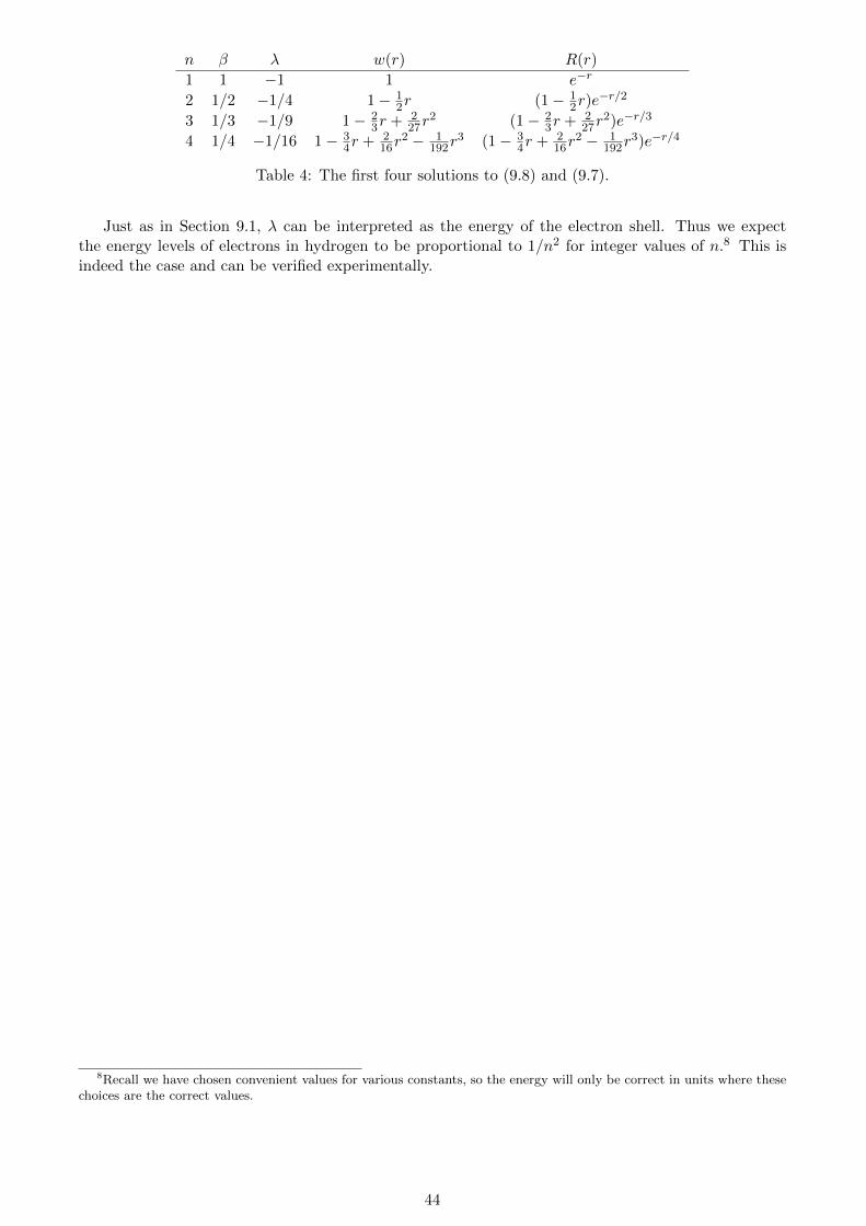
n β λ w(r) R(r)

1 1 −1 1 e−r

2 1/2 −1/4 1− 12r (1− 1

2r)e−r/2

3 1/3 −1/9 1− 23r + 2

27r2 (1− 2

3r + 227r

2)e−r/3

4 1/4 −1/16 1− 34r + 2

16r2 − 1

192r3 (1− 3

4r + 216r

2 − 1192r

3)e−r/4

Table 4: The first four solutions to (9.8) and (9.7).

Just as in Section 9.1, λ can be interpreted as the energy of the electron shell. Thus we expectthe energy levels of electrons in hydrogen to be proportional to 1/n2 for integer values of n.8 This isindeed the case and can be verified experimentally.

8Recall we have chosen convenient values for various constants, so the energy will only be correct in units where thesechoices are the correct values.

44