Part III - Advanced Probability - SRCF...Part III | Advanced Probability Based on lectures by M. Lis...
61
Part III — Advanced Probability Based on lectures by M. Lis Notes taken by Dexter Chua Michaelmas 2017 These notes are not endorsed by the lecturers, and I have modified them (often significantly) after lectures. They are nowhere near accurate representations of what was actually lectured, and in particular, all errors are almost surely mine. The aim of the course is to introduce students to advanced topics in modern probability theory. The emphasis is on tools required in the rigorous analysis of stochastic processes, such as Brownian motion, and in applications where probability theory plays an important role. Review of measure and integration: sigma-algebras, measures and filtrations; integrals and expectation; convergence theorems; product measures, independence and Fubini’s theorem. Conditional expectation: Discrete case, Gaussian case, conditional density functions; existence and uniqueness; basic properties. Martingales: Martingales and submartingales in discrete time; optional stopping; Doob’s inequalities, upcrossings, martingale convergence theorems; applications of martingale techniques. Stochastic processes in continuous time: Kolmogorov’s criterion, regularization of paths; martingales in continuous time. Weak convergence: Definitions and characterizations; convergence in distribution, tightness, Prokhorov’s theorem; characteristic functions, L´ evy’s continuity theorem. Sums of independent random variables: Strong laws of large numbers; central limit theorem; Cram´ er’s theory of large deviations. Brownian motion: Wiener’s existence theorem, scaling and symmetry properties; martingales associated with Brownian motion, the strong Markov property, hitting times; properties of sample paths, recurrence and transience; Brownian motion and the Dirichlet problem; Donsker’s invariance principle. Poisson random measures: Construction and properties; integrals. L´ evy processes: L´ evy-Khinchin theorem. Pre-requisites A basic familiarity with measure theory and the measure-theoretic formulation of probability theory is very helpful. These foundational topics will be reviewed at the beginning of the course, but students unfamiliar with them are expected to consult the literature (for instance, Williams’ book) to strengthen their understanding. 1
Transcript of Part III - Advanced Probability - SRCF...Part III | Advanced Probability Based on lectures by M. Lis...
Part III — Advanced Probability
Based on lectures by M. LisNotes taken by Dexter Chua
Michaelmas 2017
These notes are not endorsed by the lecturers, and I have modified them (oftensignificantly) after lectures. They are nowhere near accurate representations of what
was actually lectured, and in particular, all errors are almost surely mine.
The aim of the course is to introduce students to advanced topics in modern probabilitytheory. The emphasis is on tools required in the rigorous analysis of stochasticprocesses, such as Brownian motion, and in applications where probability theory playsan important role.
Review of measure and integration: sigma-algebras, measures and filtrations;integrals and expectation; convergence theorems; product measures, independence andFubini’s theorem.Conditional expectation: Discrete case, Gaussian case, conditional density functions;existence and uniqueness; basic properties.Martingales: Martingales and submartingales in discrete time; optional stopping;Doob’s inequalities, upcrossings, martingale convergence theorems; applications ofmartingale techniques.Stochastic processes in continuous time: Kolmogorov’s criterion, regularizationof paths; martingales in continuous time.Weak convergence: Definitions and characterizations; convergence in distribution,tightness, Prokhorov’s theorem; characteristic functions, Levy’s continuity theorem.Sums of independent random variables: Strong laws of large numbers; centrallimit theorem; Cramer’s theory of large deviations.Brownian motion: Wiener’s existence theorem, scaling and symmetry properties;martingales associated with Brownian motion, the strong Markov property, hittingtimes; properties of sample paths, recurrence and transience; Brownian motion and theDirichlet problem; Donsker’s invariance principle.Poisson random measures: Construction and properties; integrals.Levy processes: Levy-Khinchin theorem.
Pre-requisites
A basic familiarity with measure theory and the measure-theoretic formulation of
probability theory is very helpful. These foundational topics will be reviewed at the
beginning of the course, but students unfamiliar with them are expected to consult the
literature (for instance, Williams’ book) to strengthen their understanding.
1

Contents III Advanced Probability
Contents
0 Introduction 3
1 Some measure theory 41.1 Review of measure theory . . . . . . . . . . . . . . . . . . . . . . 41.2 Conditional expectation . . . . . . . . . . . . . . . . . . . . . . . 6
2 Martingales in discrete time 142.1 Filtrations and martingales . . . . . . . . . . . . . . . . . . . . . 142.2 Stopping time and optimal stopping . . . . . . . . . . . . . . . . 152.3 Martingale convergence theorems . . . . . . . . . . . . . . . . . . 182.4 Applications of martingales . . . . . . . . . . . . . . . . . . . . . 24
3 Continuous time stochastic processes 29
4 Weak convergence of measures 37
5 Brownian motion 425.1 Basic properties of Brownian motion . . . . . . . . . . . . . . . . 425.2 Harmonic functions and Brownian motion . . . . . . . . . . . . . 485.3 Transience and recurrence . . . . . . . . . . . . . . . . . . . . . . 525.4 Donsker’s invariance principle . . . . . . . . . . . . . . . . . . . . 53
6 Large deviations 57
Index 60
2
0 Introduction III Advanced Probability
0 Introduction
In some other places in the world, this course might be known as “StochasticProcesses”. In addition to doing probability, a new component studied in thecourse is time. We are going to study how things change over time.
In the first half of the course, we will focus on discrete time. A familiarexample is the simple random walk — we start at a point on a grid, and ateach time step, we jump to a neighbouring grid point randomly. This gives asequence of random variables indexed by discrete time steps, and are related toeach other in interesting ways. In particular, we will consider martingales, whichenjoy some really nice convergence and “stopping ”properties.
In the second half of the course, we will look at continuous time. Thereis a fundamental difference between the two, in that there is a nice topologyon the interval. This allows us to say things like we want our trajectories tobe continuous. On the other hand, this can cause some headaches because Ris uncountable. We will spend a lot of time thinking about Brownian motion,whose discovery is often attributed to Robert Brown. We can think of this as thelimit as we take finer and finer steps in a random walk. It turns out this has avery rich structure, and will tell us something about Laplace’s equation as well.
Apart from stochastic processes themselves, there are two main objects thatappear in this course. The first is the conditional expectation. Recall that if wehave a random variable X, we can obtain a number E[X], the expectation ofX. We can think of this as integrating out all the randomness of the system,and just remembering the average. Conditional expectation will be some subtlemodification of this construction, where we don’t actually get a number, butanother random variable. The idea behind this is that we want to integrate outsome of the randomness in our random variable, but keep the remaining.
Another main object is stopping time. For example, if we have a productionline that produces random number of outputs at each point, then we can ask howmuch time it takes to produce a fixed number of goods. This is a nice randomtime, which we call a stopping time. The niceness follows from the fact thatwhen the time comes, we know it. An example that is not nice is, for example,the last day it rains in Cambridge in a particular month, since on that last day,we don’t necessarily know that it is in fact the last day.
At the end of the course, we will say a little bit about large deviations.
3
1 Some measure theory III Advanced Probability
1 Some measure theory
1.1 Review of measure theory
To make the course as self-contained as possible, we shall begin with some reviewof measure theory. On the other hand, if one doesn’t already know measuretheory, they are recommended to learn the measure theory properly beforestarting this course.
Definition (σ-algebra). Let E be a set. A subset E of the power set P(E) iscalled a σ-algebra (or σ-field) if
(i) ∅ ∈ E ;
(ii) If A ∈ E , then AC = E \A ∈ E ;
(iii) If A1, A2, . . . ∈ E , then⋃∞n=1An ∈ E .
Definition (Measurable space). A measurable space is a set with a σ-algebra.
Definition (Borel σ-algebra). Let E be a topological space with topology T .Then the Borel σ-algebra B(E) on E is the σ-algebra generated by T , i.e. thesmallest σ-algebra containing T .
We are often going to look at B(R), and we will just write B for it.
Definition (Measure). A function µ : E → [0,∞] is a measure if
– µ(∅) = 0
– If A1, A2, . . . ∈ E are disjoint, then
µ
( ∞⋃i=1
Ai
)=
∞∑i=1
µ(Ai).
Definition (Measure space). A measure space is a measurable space with ameasure.
Definition (Measurable function). Let (E1, E1) and (E2, E2) be measurablespaces. Then f : E1 → E2 is said to be measurable if A ∈ E2 implies f−1(A) ∈ E1.
This is similar to the definition of a continuous function.
Notation. For (E, E) a measurable space, we write mE for the set of measurablefunctions E → R.
We write mE+ to be the positive measurable functions, which are allowed totake value ∞.
Note that we do not allow taking the values ±∞ in the first case.
Theorem. Let (E, E , µ) be a measure space. Then there exists a unique functionµ : mE+ → [0,∞] satisfying
– µ(1A) = µ(A), where 1A is the indicator function of A.
– Linearity: µ(αf + βg) = αµ(f) + βµ(g) if α, β ∈ R≥0 and f, g ∈ mE+.
4
1 Some measure theory III Advanced Probability
– Monotone convergence: iff f1, f2, . . . ∈ mE+ are such that fn f ∈ mE+
pointwise a.e. as n→∞, then
limn→∞
µ(fn) = µ(f).
We call µ the integral with respect to µ, and we will write it as µ from now on.
Definition (Simple function). A function f is simple if there exists αn ∈ R≥0
and An ∈ E for 1 ≤ n ≤ k such that
f =
k∑n=1
αn1An .
From the first two properties of the measure, we see that
µ(f) =
k∑n=1
αnµ(An).
One convenient observation is that a function is simple iff it takes on only finitelymany values. We then see that if f ∈ mE+, then
fn = 2−nb2nfc ∧ n
is a sequence of simple functions approximating f from below. Thus, givenmonotone convergence, this shows that
µ(f) = limµ(fn),
and this proves the uniqueness part of the theorem.Recall that
Definition (Almost everywhere). We say f = g almost everywhere if
µ(x ∈ E : f(x) 6= g(x)) = 0.
We say f is a version of g.
Example. Let `n = 1[n,n+1]. Then µ(`n) = 1 for all 1, but also fn → 0 andµ(0) = 0. So the “monotone” part of monotone convergence is important.
So if the sequence is not monotone, then the measure does not preserve limits,but it turns out we still have an inequality.
Lemma (Fatou’s lemma). Let fi ∈ mE+. Then
µ(
lim infn
fn
)≤ lim inf
nµ(fn).
Proof. Apply monotone convergence to the sequence infm≥n fm
Of course, it would be useful to extend integration to functions that are notnecessarily positive.
5
1 Some measure theory III Advanced Probability
Definition (Integrable function). We say a function f ∈ mE is integrable ifµ(|f |) ≤ ∞. We write L1(E) (or just L1) for the space of integrable functions.
We extend µ to L1 by
µ(f) = µ(f+)− µ(f−),
where f± = (±f) ∧ 0.
If we want to be explicit about the measure and the σ-algebra, we can writeL1(E, Eµ).
Theorem (Dominated convergence theorem). If fi ∈ mE and fi → f a.e., suchthat there exists g ∈ L1 such that |fi| ≤ g a.e. Then
µ(f) = limµ(fn).
Proof. Apply Fatou’s lemma to g − fn and g + fn.
Definition (Product σ-algebra). Let (E1, E1) and (E2, E2) be measure spaces.Then the product σ-algebraE1⊗E2 is the smallest σ-algebra on E1×E2 containingall sets of the form A1 ×A2, where Ai ∈ Ei.
Theorem. If (E1, E1, µ1) and (E2, E2, µ2) are σ-finite measure spaces, then thereexists a unique measure µ on E1 ⊗ E2) satisfying
µ(A1 ×A2) = µ1(A1)µ2(A2)
for all Ai ∈ Ei.This is called the product measure.
Theorem (Fubini’s/Tonelli’s theorem). If f = f(x1, x2) ∈ mE+ with E =E1 ⊗ E2, then the functions
x1 7→∫f(x1, x2)dµ2(x2) ∈ mE+
1
x2 7→∫f(x1, x2)dµ1(x1) ∈ mE+
2
and ∫E
f du =
∫E1
(∫E2
f(x1, x2) dµ2(x2)
)dµ1(x1)
=
∫E2
(∫E1
f(x1, x2) dµ1(x1)
)dµ2(x2)
1.2 Conditional expectation
In this course, conditional expectation is going to play an important role, andit is worth spending some time developing the theory. We are going to focuson probability theory, which, mathematically, just means we assume µ(E) = 1.Practically, it is common to change notation to E = Ω, E = F , µ = P and∫
dµ = E. Measurable functions will be written as X,Y, Z, and will be calledrandom variables. Elements in F will be called events. An element ω ∈ Ω willbe called a realization.
6
1 Some measure theory III Advanced Probability
There are many ways we can think about conditional expectations. The firstone is how most of us first encountered conditional probability.
Suppose B ∈ F , with P(B) > 0. Then the conditional probability of theevent A given B is
P(A | B) =P(A ∩B)
P(B).
This should be interpreted as the probability that A happened, given that Bhappened. Since we assume B happened, we ought to restrict to the subset of theprobability space where B in fact happened. To make this a probability space,we scale the probability measure by P(B). Then given any event A, we take theprobability of A ∩B under this probability measure, which is the formula given.
More generally, if X is a random variable, the conditional expectation of fgiven B is just the expectation under this new probability measure,
E[X | B] =E[X1B ]
P[B].
We probably already know this from high school, and we are probably not quiteexcited by this. One natural generalization would be to allow B to vary.
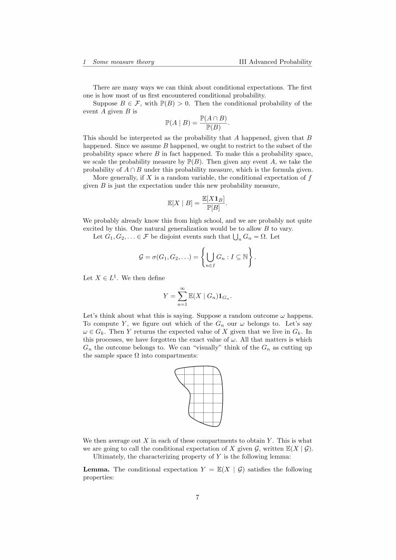
Let G1, G2, . . . ∈ F be disjoint events such that⋃nGn = Ω. Let
G = σ(G1, G2, . . .) =
⋃n∈I
Gn : I ⊆ N
.
Let X ∈ L1. We then define
Y =
∞∑n=1
E(X | Gn)1Gn.
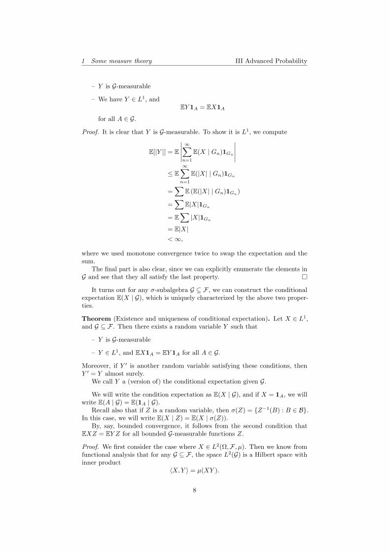
Let’s think about what this is saying. Suppose a random outcome ω happens.To compute Y , we figure out which of the Gn our ω belongs to. Let’s sayω ∈ Gk. Then Y returns the expected value of X given that we live in Gk. Inthis processes, we have forgotten the exact value of ω. All that matters is whichGn the outcome belongs to. We can “visually” think of the Gn as cutting upthe sample space Ω into compartments:
We then average out X in each of these compartments to obtain Y . This is whatwe are going to call the conditional expectation of X given G, written E(X | G).
Ultimately, the characterizing property of Y is the following lemma:
Lemma. The conditional expectation Y = E(X | G) satisfies the followingproperties:
7
1 Some measure theory III Advanced Probability
– Y is G-measurable
– We have Y ∈ L1, andEY 1A = EX1A
for all A ∈ G.
Proof. It is clear that Y is G-measurable. To show it is L1, we compute
E[|Y |] = E
∣∣∣∣∣∞∑n=1
E(X | Gn)1Gn
∣∣∣∣∣≤ E
∞∑n=1
E(|X| | Gn)1Gn
=∑
E (E(|X| | Gn)1Gn)
=∑
E|X|1Gn
= E∑|X|1Gn
= E|X|<∞,
where we used monotone convergence twice to swap the expectation and thesum.
The final part is also clear, since we can explicitly enumerate the elements inG and see that they all satisfy the last property.
It turns out for any σ-subalgebra G ⊆ F , we can construct the conditionalexpectation E(X | G), which is uniquely characterized by the above two proper-ties.
Theorem (Existence and uniqueness of conditional expectation). Let X ∈ L1,and G ⊆ F . Then there exists a random variable Y such that
– Y is G-measurable
– Y ∈ L1, and EX1A = EY 1A for all A ∈ G.
Moreover, if Y ′ is another random variable satisfying these conditions, thenY ′ = Y almost surely.
We call Y a (version of) the conditional expectation given G.
We will write the condition expectation as E(X | G), and if X = 1A, we willwrite E(A | G) = E(1A | G).
Recall also that if Z is a random variable, then σ(Z) = Z−1(B) : B ∈ B.In this case, we will write E(X | Z) = E(X | σ(Z)).
By, say, bounded convergence, it follows from the second condition thatEXZ = EY Z for all bounded G-measurable functions Z.
Proof. We first consider the case where X ∈ L2(Ω,F , µ). Then we know fromfunctional analysis that for any G ⊆ F , the space L2(G) is a Hilbert space withinner product
〈X,Y 〉 = µ(XY ).
8
1 Some measure theory III Advanced Probability
In particular, L2(G) is a closed subspace of L2(F). We can then define Y tobe the orthogonal projection of X onto L2(G). It is immediate that Y is G-measurable. For the second part, we use that X − Y is orthogonal to L2(G),since that’s what orthogonal projection is supposed to be. So E(X − Y )Z = 0for all Z ∈ L2(G). In particular, since the measure space is finite, the indicatorfunction of any measurable subset is L2. So we are done.
We next focus on the case where X ∈ mE+. We define
Xn = X ∧ n
We want to use monotone convergence to obtain our result. To do so, we needthe following result:
Claim. If (X,Y ) and (X ′, Y ′) satisfy the conditions of the theorem, and X ′ ≥ Xa.s., then Y ′ ≥ Y a.s.
Proof. Define the event A = Y ′ ≤ Y ∈ G. Consider the event Z = (Y −Y ′)1A.Then Z ≥ 0. We then have
EY ′1A = EX ′1A ≥ EX1A = EY 1A.
So it follows that we also have E(Y − Y ′)1A ≤ 0. So in fact EZ = 0. So Y ′ ≥ Ya.s.
We can now define Yn = E(Xn | G), picking them so that Yn is increasing.We then take Y∞ = limYn. Then Y∞ is certainly G-measurable, and by monotoneconvergence, if A ∈ G, then
EX1A = limEXn1A = limEYn1A = EY∞1A.
Now if EX <∞, then EY∞ = EX <∞. So we know Y∞ is finite a.s., and wecan define Y = Y∞1Y∞<∞.
Finally, we work with arbitrary X ∈ L1. We can write X = X+ −X−, andthen define Y ± = E(X± | G), and take Y = Y + − Y −.
Uniqueness is then clear.
Lemma. If Y is σ(Z)-measurable, then there exists h : R→ R Borel-measurablesuch that Y = h(Z). In particular,
E(X | Z) = h(Z) a.s.
for some h : R→ R.
We can then define E(X | Z = z) = h(z). The point of doing this is that wewant to allow for the case where in fact we have P(Z = z) = 0, in which caseour original definition does not make sense.
Exercise. Consider X ∈ L1, and Z : Ω→ N discrete. Compute E(X | Z) andcompare our different definitions of conditional expectation.
Example. Let (U, V ) ∈ R2 with density fU,V (u, v), so that for any B1, B2 ∈ B,we have
P(U ∈ B1, V ∈ B2) =
∫B1
∫b2
fU,V (u, v) du dv.
9
1 Some measure theory III Advanced Probability
We want to compute E(h(V ) | U), where h : R → R is Borel measurable. Wecan define
fU (u) =
∫RfU,V (u, v) dv,
and we define the conditional density of V given U by
F|U (v | u) =fU,V (u, v)
fU (u).
We define
g(u) =
∫h(u)fV |U (v | u) dv.
We claim that E(h(V ) | U) is just g(U).To check this, we show that it satisfies the two desired conditions. It is clear
that it is σ(U)-measurable. To check the second condition, fix an A ∈ σ(U).Then A = (u, v) : u ∈ B for some B. Then
E(h(V )1A) =
∫∫h(v)1u∈BfU,V (u, v) du dv
=
∫∫h(v)1u∈BfV |U (v | u)fV (u) du dv
=
∫g(U)1u∈BfU (u) du
= E(g(U)1A),
as desired.
The point of this example is that to compute conditional expectations, weuse our intuition to guess what the conditional expectation should be, and thencheck that it satisfies the two uniquely characterizing properties.
Example. Suppose (X,W ) are Gaussian. Then for all linear functions ϕ : R2 →R, the quantity ϕ(X,W ) is Gaussian.
One nice property of Gaussians is that lack of correlation implies independence.We want to compute E(X |W ). Note that if Y is such that EX = EY , X − Yis independent of W , and Y is W -measurable, then Y = E(X | W ), sinceE(X − Y )1A = 0 for all σ(W )-measurable A.
The guess is that we want Y to be a Gaussian variable. We put Y = aW + b.Then EX = EY implies we must have
aEW + b = EX. (∗)
The independence part requires cov(X − Y,W ) = 0. Since covariance is linear,we have
0 = cov(X−Y,W ) = cov(X,W )−cov(aW +b,W ) = cov(X,W )−a cov(W,W ).
Recalling that cov(W,W ) = var(W ), we need
a =cov(X,W )
var(W ).
This then allows us to use (∗) to compute b as well. This is how we compute theconditional expectation of Gaussians.
10
1 Some measure theory III Advanced Probability
We note some immediate properties of conditional expectation. As usual,all (in)equality and convergence statements are to be taken with the quantifier“almost surely”.
Proposition.
(i) E(X | G) = X iff X is G-measurable.
(ii) E(E(X | G)) = EX
(iii) If X ≥ 0 a.s., then E(X | G) ≥ 0
(iv) If X and G are independent, then E(X | G) = E[X]
(v) If α, β ∈ R and X1, X2 ∈ L1, then
E(αX1 + βX2 | G) = αE(X1 | G) + βE(X2 | G).
(vi) Suppose Xn X. Then
E(Xn | G) E(X | G).
(vii) Fatou’s lemma: If Xn are non-negative measurable, then
E(
lim infn→∞
Xn | G)≤ lim inf
n→∞E(Xn | G).
(viii) Dominated convergence theorem: If Xn → X and Y ∈ L1 such thatY ≥ |Xn| for all n, then
E(Xn | G)→ E(X | G).
(ix) Jensen’s inequality : If c : R→ R is convex, then
E(c(X) | G) ≥ c(E(X) | G).
(x) Tower property : If H ⊆ G, then
E(E(X | G) | H) = E(X | H).
(xi) For p ≥ 1,‖E(X | G)‖p ≤ ‖X‖p.
(xii) If Z is bounded and G-measurable, then
E(ZX | G) = ZE(X | G).
(xiii) Let X ∈ L1 and G,H ⊆ F . Assume that σ(X,G) is independent of H.Then
E(X | G) = E(X | σ(G,H)).
Proof.
(i) Clear.
11
1 Some measure theory III Advanced Probability
(ii) Take A = ω.
(iii) Shown in the proof.
(iv) Clear by property of expected value of independent variables.
(v) Clear, since the RHS satisfies the unique characterizing property of theLHS.
(vi) Clear from construction.
(vii) Same as the unconditional proof, using the previous property.
(viii) Same as the unconditional proof, using the previous property.
(ix) Same as the unconditional proof.
(x) The LHS satisfies the characterizing property of the RHS
(xi) Using the convexity of |x|p, Jensen’s inequality tells us
‖E(X | G)‖pp = E|E(X | G)|p
≤ E(E(|X|p | G))
= E|X|p
= ‖X‖pp
(xii) If Z = 1B , and let b ∈ G. Then
E(ZE(X | G)1A) = E(E(X | G) · 1A∩B) = E(X1A∩B) = E(ZX1A).
So the lemma holds. Linearity then implies the result for Z simple, thenapply our favorite convergence theorems.
(xiii) Take B ∈ H and A ∈ G. Then
E(E(X | σ(G,H)) · 1A∩B) = E(X · 1A∩B)
= E(X1A)P(B)
= E(E(X | G)1A)P(B)
= E(E(X | G)1A∩B)
If instead of A ∩ B, we had any σ(G,H)-measurable set, then we wouldbe done. But we are fine, since the set of subsets of the form A ∩B withA ∈ G, B ∈ H is a generating π-system for σ(H,G).
We shall end with the following key lemma. We will later use it to show thatmany of our martingales are uniformly integrable.
Lemma. If X ∈ L1, then the family of random variables YG = E(X | G) for allG ⊆ F is uniformly integrable.
In other words, for all ε > 0, there exists λ > 0 such that
E(YG1|YG>λ|) < ε
for all G.
12
1 Some measure theory III Advanced Probability
Proof. Fix ε > 0. Then there exists δ > 0 such that E|X|1A < ε for any A withP(A) < δ.
Take Y = E(X | G). Then by Jensen, we know
|Y | ≤ E(|X| | G)
In particular, we haveE|Y | ≤ E|X|.
By Markov’s inequality, we have
P(|Y | ≥ λ) ≤ E|Y |λ≤ E|X|
λ.
So take λ such that E|X|λ < δ. So we have
E(|Y |1|Y |≥λ) ≤ E(E(|X| | G)1|Y |≥λ) = E(|X|1|Y |≥λ) < ε
using that 1|Y |≥λ is a G-measurable function.
13
2 Martingales in discrete time III Advanced Probability
2 Martingales in discrete time
2.1 Filtrations and martingales
We would like to model some random variable that “evolves with time”. Forexample, in a simple random walk, Xn could be the position we are at time n.To do so, we would like to have some σ-algebras Fn that tells us the “informationwe have at time n”. This structure is known as a filtration.
Definition (Filtration). A filtration is a sequence of σ-algebras (Fn)n≥0 suchthat F ⊇ Fn+1 ⊇ Fn for all n. We define F∞ = σ(F0,F1, . . .) ⊆ F .
We will from now on assume (Ω,F ,P) is equipped with a filtration (Fn)n≥0.
Definition (Stochastic process in discrete time). A stochastic process (in discretetime) is a sequence of random variables (Xn)n≥0.
This is a very general definition, and in most cases, we would want Xn tointeract nicely with our filtration.
Definition (Natural filtration). The natural filtration of (Xn)n≥0 is given by
FXn = σ(X1, . . . , Xn).
Definition (Adapted process). We say that (Xn)n≥0 is adapted (to (Fn)n≥0)if Xn is Fn-measurable for all n ≥ 0. Equivalently, if FXn ⊆ Fn.
Definition (Integrable process). A process (Xn)n≥0 is integrable if Xn ∈ L1 forall n ≥ 0.
We can now write down the definition of a martingale.
Definition (Martingale). An integrable adapted process (Xn)n≥0 is a martingaleif for all n ≥ m, we have
E(Xn | Fm) = Xm.
We say it is a super-martingale if
E(Xn | Fm) ≤ Xm,
and a sub-martingale ifE(Xn | Fm) ≥ Xm,
Note that it is enough to take m = n − 1 for all n ≥ 0, using the towerproperty.
The idea of a martingale is that we cannot predict whether Xn will go upor go down in the future even if we have all the information up to the present.For example, if Xn denotes the wealth of a gambler in a gambling game, then insome sense (Xn)n≥0 being a martingale means the game is “fair” (in the senseof a fair dice).
Note that (Xn)n≥0 is a super-martingale iff (−Xn)n≥0 is a sub-martingale,and if (Xn)n≥0 is a martingale, then it is both a super-martingale and a sub-martingale. Often, what these extra notions buy us is that we can formulateour results for super-martingales (or sub-martingales), and then by applying theresult to both (Xn)n≥0 and (−Xn)n≥0, we obtain the desired, stronger resultfor martingales.
14

2 Martingales in discrete time III Advanced Probability
2.2 Stopping time and optimal stopping
The optional stopping theorem says the definition of a martingale in fact impliesan a priori much stronger property. To formulate the optional stopping theorem,we need the notion of a stopping time.
Definition (Stopping time). A stopping time is a random variable T : Ω →N≥0 ∪ ∞ such that
T ≤ n ∈ Fnfor all n ≥ 0.
This means that at time n, if we want to know if T has occurred, we candetermine it using the information we have at time n.
Note that T is a stopping time iff t = n ∈ Fn for all n, since if T is astopping time, then
T = n = T ≤ n \ T ≤ n− 1,
and T ≤ n− 1 ∈ Fn−1 ⊆ Fn. Conversely,
T ≤ n =
n⋃k=1
T = k ∈ Fn.
This will not be true in the continuous case.
Example. If B ∈ B(R), then we can define
T = infn : Xn ∈ B.
Then this is a stopping time.On the other hand,
T = supn : Xn ∈ B
is not a stopping time (in general).
Given a stopping time, we can make the following definition:
Definition (XT ). For a stopping time T , we define the random variable XT by
XT (ω) = XT (ω)(ω)
on T <∞, and 0 otherwise.
Later, for suitable martingales, we will see that the limit X∞ = limn→∞Xn
makes sense. In that case, We define XT (ω) to be X∞(ω) if T =∞.Similarly, we can define
Definition (Stopped process). The stopped process is defined by
(XTn )n≥0 = (XT (ω)∧n(ω))n≥0.
This says we stop evolving the random variable X once T has occurred.We would like to say that XT is “FT -measurable”, i.e. to compute XT , we
only need to know the information up to time T . After some thought, we seethat the following is the correct definition of FT :
15
2 Martingales in discrete time III Advanced Probability
Definition (FT ). For a stopping time T , define
FT = A ∈ F∞ : A ∩ T ≤ n ∈ Fn.
This is easily seen to be a σ-algebra.
Example. If T ≡ n is constant, then FT = Fn.
There are some fairly immediate properties of these objects, whose proof isleft as an exercise for the reader:
Proposition.
(i) If T, S, (Tn)n≥0 are all stopping times, then
T ∨ S, T ∧ S, supnTn, inf Tn, lim supTn, lim inf Tn
are all stopping times.
(ii) FT is a σ-algebra
(iii) If S ≤ T , then FS ⊆ FT .
(iv) XT1T<∞ is FT -measurable.
(v) If (Xn) is an adapted process, then so is (XTn )n≥0 for any stopping time T .
(vi) If (Xn) is an integrable process, then so is (XTn )n≥0 for any stopping time
T .
We now come to the fundamental property of martingales.
Theorem (Optional stopping theorem). Let (Xn)n≥0 be a super-martingaleand S ≤ T bounded stopping times. Then
EXT ≤ EXS .
Proof. Follows from the next theorem.
What does this theorem mean? If X is a martingale, then it is both asuper-martingale and a sub-martingale. So we can apply this to both X and−X, and so we have
E(XT ) = E(XS).
In particular, since 0 is a stopping time, we see that
EXT = EX0
for any bounded stopping time T .Recall that martingales are supposed to model fair games. If we again think
of Xn as the wealth at time n, and T as the time we stop gambling, then thissays no matter how we choose T , as long as it is bounded, the expected wealthat the end is the same as what we started with.
16
2 Martingales in discrete time III Advanced Probability
Example. Consider the stopping time
T = infn : Xn = 1,
and take X such that EX0 = 0. Then clearly we have EXT = 1. So this tells usT is not a bounded stopping time!
Theorem. The following are equivalent:
(i) (Xn)n≥0 is a super-martingale.
(ii) For any bounded stopping times T and any stopping time S,
E(XT | FS) ≤ XS∧T .
(iii) (XTn ) is a super-martingale for any stopping time T .
(iv) For bounded stopping times S, T such that S ≤ T , we have
EXT ≤ EXS .
In particular, (iv) implies (i).
Proof.
– (ii) ⇒ (iii): Consider (XT ′
n )≥0 for a stopping time T ′. To check if this is asuper-martingale, we need to prove that whenever m ≤ n,
E(Xn∧T ′ | Fm) ≤ Xm∧T ′ .
But this follows from (ii) above by taking S = m and T = T ′ ∧ n.
– (ii) ⇒ (iv): Clear by the tower law.
– (iii) ⇒ (i): Take T =∞.
– (i) ⇒ (ii): Assume T ≤ n. Then
XT = XS∧T +∑
S≤k<T
(Xk+1 −Xk)
= XS∧T +
n∑k=0
(Xk+1 −Xk)1S≤k<T (∗)
Now note that S ≤ k < T = S ≤ k ∩ T ≤ kc ∈ Fk. Let A ∈ FS .Then A ∩ S ≤ k ∈ Fk by definition of FS . So A ∩ S ≤ k < T ∈ Fk.
Apply E to to (∗)× 1A. Then we have
E(XT1A) = E(XS∧T1A) +
n∑k=0
E(Xk+1 −Xk)1A∩S≤k<T.
But for all k, we know
E(Xk+1 −Xk)1A∩S≤k<T ≤ 0,
17
2 Martingales in discrete time III Advanced Probability
since X is a super-martingale. So it follows that for all A ∈ FS , we have
E(XT · 1A) ≤ E(XS∧T1A).
But since XS∧T is FS∧T measurable, it is in particular FS measurable. Soit follows that for all A ∈ FS , we have
E(E(XT | FS)1A) ≤ E(XS∧T1A).
So the result follows.
– (iv) ⇒ (i): Fix m ≤ n and A ∈ Fm. Take
T = m1A + 1AC .
One then manually checks that this is a stopping time. Now note that
XT = Xm1A +Xn1AC .
So we have
0 ≥ E(Xn)− E(XT )
= E(Xn)− E(Xn1Ac)− E(Xm1A)
= E(Xn1A)− E(Xm1A).
Then the same argument as before gives the result.
2.3 Martingale convergence theorems
One particularly nice property of martingales is that they have nice conver-gence properties. We shall begin by proving a pointwise version of martingaleconvergence.
Theorem (Almost sure martingale convergence theorem). Suppose (Xn)n≥0
is a super-martingale that is bounded in L1, i.e. supn E|Xn| <∞. Then thereexists an F∞-measurable X∞ ∈ L1 such that
Xn → X∞ a.s. as n→∞.
To begin, we need a convenient characterization of when a series converges.
Definition (Upcrossing). Let (xn) be a sequence and (a, b) an interval. Anupcrossing of (a, b) by (xn) is a sequence j, j + 1, . . . , k such that xj ≤ a andxk ≥ b. We define
Un[a, b, (xn)] = number of disjoint upcrossings contained in 1, . . . , nU [a, b, (xn)] = lim
n→∞Un[a, b, x].
We can then make the following elementary observation:
Lemma. Let (xn)n≥0 be a sequence of numbers. Then xn converges in R if andonly if
(i) lim inf |xn| <∞.
18
2 Martingales in discrete time III Advanced Probability
(ii) For all a, b ∈ Q with a < b, we have U [a, b, (xn)] <∞.
For our martingales, since they are bounded in L1, Fatou’s lemma tells usE lim inf |Xn| <∞. So lim inf |Xn| = 0 almost surely. Thus, it remains to showthat for any fixed a < b ∈ Q, we have P(U [a, b, (Xn)] = ∞) = 0. This is aconsequence of Doob’s upcrossing lemma.
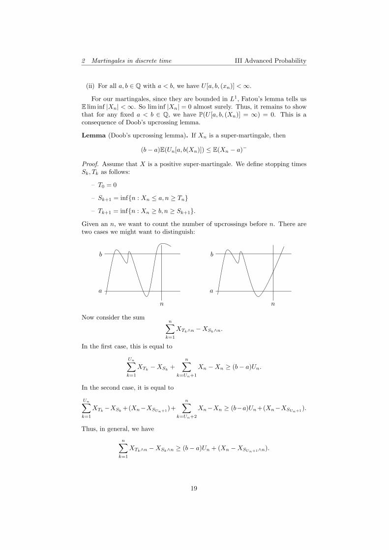
Lemma (Doob’s upcrossing lemma). If Xn is a super-martingale, then
(b− a)E(Un[a, b(Xn)]) ≤ E(Xn − a)−
Proof. Assume that X is a positive super-martingale. We define stopping timesSk, Tk as follows:
– T0 = 0
– Sk+1 = infn : Xn ≤ a, n ≥ Tn
– Tk+1 = infn : Xn ≥ b, n ≥ Sk+1.
Given an n, we want to count the number of upcrossings before n. There aretwo cases we might want to distinguish:
b
a
n
b
a
n
Now consider the sumn∑k=1
XTk∧n −XSk∧n.
In the first case, this is equal to
Un∑k=1
XTk−XSk
+
n∑k=Un+1
Xn −Xn ≥ (b− a)Un.
In the second case, it is equal to
Un∑k=1
XTk−XSk
+(Xn−XSUn+1)+
n∑k=Un+2
Xn−Xn ≥ (b−a)Un+(Xn−XSUn+1).
Thus, in general, we have
n∑k=1
XTk∧n −XSk∧n ≥ (b− a)Un + (Xn −XSUn+1∧n).
19
2 Martingales in discrete time III Advanced Probability
By definition, Sk < Tk ≤ n. So the expectation of the LHS is always non-negativeby super-martingale convergence, and thus
0 ≥ (b− a)EUn + E(Xn −XSUn+1∧n).
Then observe thatXn −XSUn+1
≥ −(Xn − a)−.
The almost-sure martingale convergence theorem is very nice, but often it isnot good enough. For example, we might want convergence in Lp instead. Thefollowing example shows this isn’t always possible:
Example. Suppose (ρn)n≥0 is a sequence of iid random variables and
P(ρn = 0) =1
2= P(ρn = 2).
Let
Xn =
n∏k=0
ρk.
Then this is a martingale, and EXn = 1. On the other hand, Xn → 0 almostsurely. So ‖Xn −X∞‖1 does not converge to 0.
For p > 1, if we want convergence in Lp, it is not surprising that we at leastneed the sequence to be Lp bounded. We will see that this is in fact sufficient.For p = 1, however, we need a bit more than being bounded in L1. We will needuniform integrability.
To prove this, we need to establish some inequalities.
Lemma (Maximal inequality). Let (Xn) be a sub-martingale that is non-negative, or a martingale. Define
X∗n = supk≤n|Xk|, X∗ = lim
n→∞X∗n.
If λ ≥ 0, thenλP(X∗n ≥ λ) ≤ E[|Xn|1X∗n≥λ].
In particular, we haveλP(X∗n ≥ λ) ≤ E[|Xn|].
Markov’s inequality says almost the same thing, but has E[|X∗n|] instead ofE[|Xn|]. So this is a stronger inequality.
Proof. If Xn is a martingale, then |Xn| is a sub-martingale. So it suffices toconsider the case of a non-negative sub-martingale. We define the stopping time
T = infn : Xn ≥ λ.
By optional stopping,
EXn ≥ EXT∧n
= EXT1T≤n + EXn1T>n
≥ λP(T ≤ n) + EXn1T>n
= λP(X∗n ≥ λ) + EXn1T>n.
20
2 Martingales in discrete time III Advanced Probability
Lemma (Doob’s Lp inequality). For p > 1, we have
‖X∗n‖p ≤p
p− 1‖Xn‖p
for all n.
Proof. Let k > 0, and consider
‖X∗n ∧ k‖pp = E|X∗n ∧ k|p.
We use the fact that
xp =
∫ x
0
psp−1 ds.
So we have
‖X∗n ∧ k‖pp = E|X∗n ∧ k|p
= E∫ X∗n∧k
0
pxp−1 dx
= E∫ k
0
pxp−11X∗n≥x dx
=
∫ k
0
pxp−1P(X∗n ≥ x) dx (Fubini)
≤∫ k
0
pxp−2EXn1X∗n≥x dx (maximal inequality)
= EXn
∫ k
0
pxp−21X∗n≥x dx (Fubini)
=p
p− 1EXn(X∗n ∧ k)p−1
≤ p
p− 1‖Xn‖p (E(X∗n ∧ k)p)
p−1p (H older)
=p
p− 1‖Xn‖p‖X∗n ∧ k‖p−1
p
Now take the limit k →∞ and divide by ‖X∗n‖p−1p .
Theorem (Lp martingale convergence theorem). Let (Xn)n≥0 be a martingale,and p > 1. Then the following are equivalent:
(i) (Xn)n≥0 is bounded in Lp, i.e. supn E|Xi|p <∞.
(ii) (Xn)n≥0 converges as n→∞ to a random variable X∞ ∈ Lp almost surelyand in Lp.
(iii) There exists a random variable Z ∈ Lp such that
Xn = E(Z | Fn)
Moreover, in (iii), we always have X∞ = E(Z | F∞).
This gives a bijection between martingales bounded in Lp and Lp(F∞),sending (Xn)n≥0 7→ X∞.
21
2 Martingales in discrete time III Advanced Probability
Proof.
– (i) ⇒ (ii): If (Xn)n≥0 is bounded in Lp, then it is bounded in L1. So bythe martingale convergence theorem, we know (Xn)n≥0 converges almostsurely to X∞. By Fatou’s lemma, we have X∞ ∈ Lp.Now by monotone convergence, we have
‖X∗‖p = limn‖X∗n‖p ≤
p
p− 1supn‖Xn‖p <∞.
By the triangle inequality, we have
|Xn −X∞| ≤ 2X∗ a.s.
So by dominated convergence, we know that Xn → X∞ in Lp.
– (ii) ⇒ (iii): Take Z = X∞. We want to prove that
Xm = E(X∞ | Fm).
To do so, we show that ‖Xm − E(X∞ | Fm)‖p = 0. For n ≥ m, we knowthis is equal to
‖E(Xn | Fm)−E(X∞ | Fm)‖p = ‖E(Xn−X∞ | Fm)‖p ≤ ‖Xn−X∞‖p → 0
as n→∞, where the last step uses Jensen’s. But it is also a constant. Sowe are done.
– (iii) ⇒ (i): Since expectation decreases Lp norms, we already know that(Xn)n≥0 is Lp-bounded.
To show the “moreover” part, note that⋃n≥0 Fn is a π-system that
generates F∞. So it is enough to prove that
EX∞1A = E(E(Z | F∞)1A).
But if A ∈ FN , then
EX∞1A = limn→∞
EXn1A
= limn→∞
E(E(Z | Fn)1A)
= limn→∞
E(E(Z | F∞)1A),
where the last step relies on the fact that 1A is Fn-measurable.
We finally finish off the p = 1 case with the additional uniform integrabilitycondition.
Theorem (Convergence in L1). Let (Xn)n≥0 be a martingale. Then the follow-ing are equivalent:
(i) (Xn)n≥0 is uniformly integrable.
(ii) (Xn)n≥0 converges almost surely and in L1.
(iii) There exists Z ∈ L1 such that Xn = E(Z | Fn) almost surely.
22
2 Martingales in discrete time III Advanced Probability
Moreover, X∞ = E(Z | F∞).
The proof is very similar to the Lp case.
Proof.
– (i)⇒ (ii): Let (Xn)n≥0 be uniformly integrable. Then (Xn)n≥0 is boundedin L1. So the (Xn)n≥0 converges to X∞ almost surely. Then by measuretheory, uniform integrability implies that in fact Xn → L1.
– (ii) ⇒ (iii): Same as the Lp case.
– (iii) ⇒ (i): For any Z ∈ L1, the collection E(Z | G) ranging over allσ-subalgebras G is uniformly integrable.
Thus, there is a bijection between uniformly integrable martingales andL1(F∞).
We now revisit optional stopping for uniformly integrable martingales. Recallthat in the statement of optional stopping, we needed our stopping times to bebounded. It turns out if we require our martingales to be uniformly integrable,then we can drop this requirement.
Theorem. If (Xn)n≥0 is a uniformly integrable martingale, and S, T are arbi-trary stopping times, then E(XT | FS) = XS∧T . In particular EXT = X0.
Note that we are now allowing arbitrary stopping times, so T may be infinitewith non-zero probability. Hence we define
XT =
∞∑n=0
Xn1T=n +X∞1T=∞.
Proof. By optional stopping, for every n, we know that
E(XT∧n | FS) = XS∧T∧n.
We want to be able to take the limit as n → ∞. To do so, we need to showthat things are uniformly integrable. First, we apply optional stopping to writeXT∧n as
XT∧n = E(Xn | FT∧n)
= E(E(X∞ | Fn) | FT∧n)
= E(X∞ | FT∧n).
So we know (XTn )n≥0 is uniformly integrable, and hence Xn∧T → XT almost
surely and in L1.To understand E(XT∧n | FS), we note that
‖E(Xn∧T −XT | FS)‖1 ≤ ‖Xn∧T −XT ‖1 → 0 as n→∞.
So it follows that E(Xn∧T | FS)→ E(XT | FS) as n→∞.
23

2 Martingales in discrete time III Advanced Probability
2.4 Applications of martingales
Having developed the theory, let us move on to some applications. Before we dothat, we need the notion of a backwards martingale.
Definition (Backwards filtration). A backwards filtration on a measurable space(E, E) is a sequence of σ-algebras Fn ⊆ E such that Fn+1 ⊆ Fn. We define
F∞ =⋂n≥0
Fn.
Theorem. Let Y ∈ L1, and let Fn be a backwards filtration. Then
E(Y | Fn)→ E(Y | F∞)
almost surely and in L1.
A process of this form is known as a backwards martingale.
Proof. We first show that E(Y | Fn) converges. We then show that what itconverges to is indeed E(Y | F∞).
We writeXn = E(Y | Fn).
Observe that for all n ≥ 0, the process (Xn−k)0≤k≤n is a martingale by the towerproperty, and so is (−Xn−k)0≤k≤n. Now notice that for all a < b, the numberof upcrossings of [a, b] by (Xk)0≤k≤n is equal to the number of upcrossings of[−b,−a] by (−Xn−k)0≤k≤n.
Using the same arguments as for martingales, we conclude that Xn → X∞almost surely and in L1 for some X∞.
To see that X∞ = E(Y | F∞), we notice that X∞ is F∞ measurable. So it isenough to prove that
EX∞1A = E(E(Y | F∞)1A)
for all A ∈ F∞. Indeed, we have
EX∞1A = limn→∞
EXn1A
= limn→∞
E(E(Y | Fn)1A)
= limn→∞
E(Y | 1A)
= E(Y | 1A)
= E(E(Y | Fn)1A).
Theorem (Kolmogorov 0-1 law). Let (Xn)n≥0 be independent random variables.Then, let
Fn = σ(Xn+1, Xn+2, . . .).
Then the tail σ-algebra F∞ is trivial, i.e. P(A) ∈ 0, 1 for all A ∈ F∞.
Proof. Let Fn = σ(X1, . . . , Xn). Then Fn and Fn are independent. Then forall A ∈ F∞, we have
E(1A | Fn) = P(A).
But the LHS is a martingale. So it converges almost surely and in L1 toE(1A | F∞). But 1A is F∞-measurable, since F∞ ⊆ F∞. So this is just 1A. So1A = P(A) almost surely, and we are done.
24
2 Martingales in discrete time III Advanced Probability
Theorem (Strong law of large numbers). Let (Xn)n≥1 be iid random variablesin L1, with EX1 = µ. Define
Sn =
n∑i=1
Xi.
ThenSnn→ µ as n→∞
almost surely and in L1.
Proof. We have
Sn = E(Sn | Sn) =
n∑i=1
E(Xi | Sn) = nE(X1 | Sn).
So the problem is equivalent to showing that E(X1 | Sn)→ µ as n→∞. Thisseems like something we can tackle with our existing technology, except that theSn do not form a filtration.
Thus, define a backwards filtration
Fn = σ(Sn, Sn+1, Sn+2, . . .) = σ(Sn, Xn+1, Xn+2, . . .) = σ(Sn, τn),
where τn = σ(Xn+1, Xn+2, . . .). We now use the property of conditional expec-tation that we’ve never used so far, that adding independent information to aconditional expectation doesn’t change the result. Since τn is independent ofσ(X1, Sn), we know
Snn
= E(X1 | Sn) = E(X1 | Fn).
Thus, by backwards martingale convergence, we know
Snn→ E(X1 | F∞).
But by the Kolmogorov 0-1 law, we know F∞ is trivial. So we know that E(X1 |F∞) is almost constant, which has to be E(E(X1 | F∞)) = E(X1) = µ.
Recall that if (E, E , µ) is a measure space and f ∈ mE+, then
ν(A) = µ(f1A)
is a measure on E . We say f is a density of ν with respect to µ.We can ask an “inverse” question – given two different measures on E , when
is it the case that one is given by a density with respect to the other?A first observation is that if ν(A) = µ(f1A), then whenever µ(A) = 0, we
must have ν(A) = 0. However, this is not sufficient. For example, let µ be acounting measure on R, and ν the Lebesgue measure. Then our condition issatisfied. However, if ν is given by a density f with respect to ν, we must have
0 = ν(x) = µ(f1x) = f(x).
So f ≡ 0, but taking f ≡ 0 clearly doesn’t give the Lebesgue measure.The problem with this is that µ is not a σ-finite measure.
25
2 Martingales in discrete time III Advanced Probability
Theorem (Radon–Nikodym). Let (Ω,F) be a measurable space, and Q and Pbe two probability measures on (Ω,F). Then the following are equivalent:
(i) Q is absolutely continuous with respect to P, i.e. for any A ∈ F , if P(A) = 0,then Q(A) = 0.
(ii) For any ε > 0, there exists δ > 0 such that for all A ∈ F , if P(A) ≤ δ, thenQ(A) ≤ ε.
(iii) There exists a random variable X ≥ 0 such that
Q(A) = EP(X1A).
In this case, X is called the Radon–Nikodym derivative of Q with respectto P, and we write X = dQ
dP .
Note that this theorem works for all finite measures by scaling, and thus forσ-finite measures by partitioning Ω into sets of finite measure.
Proof. We shall only treat the case where F is countably generated , i.e. F =σ(F1, F2, . . .) for some sets Fi. For example, any second-countable topologicalspace is countably generated.
– (iii) ⇒ (i): Clear.
– (ii) ⇒ (iii): Define the filtration
Fn = σ(F1, F2, . . . , Fn).
Since Fn is finite, we can write it as
Fn = σ(An,1, . . . , An,mn),
where each An,i is an atom, i.e. if B ( An,i and B ∈ Fn, then B = ∅. Wedefine
Xn =
mn∑n=1
Q(An,i)
P(An,i)1An,i ,
where we skip over the terms where P(An,i) = 0. Note that this is exactlydesigned so that for any A ∈ Fn, we have
EP(Xn1A) = EP∑
An,i⊆A
Q(An,i)
P(An, i)1An,i
= Q(A).
Thus, if A ∈ Fn ⊆ Fn+1, we have
EXn+11A = Q(A) = EXn1A.
So we know thatE(Xn+1 | Fn) = Xn.
It is also immediate that (Xn)n≥0 is adapted. So it is a martingale.
We next show that (Xn)n≥0 is uniformly integrable. By Markov’s inequality,we have
P(Xn ≥ λ) ≤ EXn
λ=
1
λ≤ δ
26
2 Martingales in discrete time III Advanced Probability
for λ large enough. Then
E(Xn1Xn≥λ) = Q(Xn ≥ λ) ≤ ε.
So we have shown uniform integrability, and so we know Xn → X almostsurely and in L1 for some X. Then for all A ∈
⋃n≥0 Fn, we have
Q(A) = limn→∞
EXn1A = EX1A.
So Q(−) and EX1(−) agree on⋃n≥0 Fn, which is a generating π-system
for F , so they must be the same.
– (i) ⇒ (ii): Suppose not. Then there exists some ε > 0 and someA1, A2, . . . ∈ F such that
Q(An) ≥ ε, P(An) ≤ 1
2n.
Since∑n P(An) is finite, by Borel–Cantelli, we know
P lim supAn = 0.
On the other hand, by, say, dominated convergence, we have
Q lim supAn = Q
( ∞⋂n=1
∞⋃m=n
Am
)
= limk→∞
Q
(k⋂
n=1
∞⋃m=n
Am
)
≥ limk→∞
Q
( ∞⋃m=k
Ak
)≥ ε.
This is a contradiction.
Finally, we end the part on discrete time processes by relating what we havedone to Markov chains.
Let’s first recall what Markov chains are. Let E be a countable space, and µa measure on E. We write µx = µ(x), and then µ(f) = µ · f .
Definition (Transition matrix). A transition matrix is a matrix P = (pxy)x,y∈Esuch that each px = (px,y)y∈E is a probability measure on E.
Definition (Markov chain). An adapted process (Xn) is called a Markov chainif for any n and A ∈ Fn such that xn = x ⊇ A, we have
P(Xn+1 = y | A) = pxy.
Definition (Harmonic function). A function f : E → R is harmonic if Pf = f .In other words, for any x, we have∑
y
pxyf(y) = f(x).
27
2 Martingales in discrete time III Advanced Probability
We then observe that
Proposition. If F is harmonic and bounded, and (Xn)n≥0 is Markov, then(f(Xn))n≥0 is a martingale.
Example. Let (Xn)n≥0 be iid Z-valued random variables in L1, and E[Xi] = 0.Then
Sn = X0 + · · ·+Xn
is a martingale and a Markov chain.However, if Z is a Z-valued random variable, consider the random variable
(ZSn)n≥0 and Fn = σ(Fn, Z). Then this is a martingale but not a Markovchain.
28
3 Continuous time stochastic processes III Advanced Probability
3 Continuous time stochastic processes
In the remainder of the course, we shall study continuous time processes. Whendoing so, we have to be rather careful, since our processes are index by anuncountable set, when measure theory tends to only like countable things. Ul-timately, we would like to study Brownian motion, but we first develop somegeneral theory of continuous time processes.
Definition (Continuous time stochastic process). A continuous time stochasticprocess is a family of random variables (Xt)t≥0 (or (Xt)t∈[a,b]).
In the discrete case, if T is a random variable taking values in 0, 1, 2, . . .,then it makes sense to look at the new random variable XT , since this is just
XT =
∞∑n=0
Xn1T=n.
This is obviously measurable, since it is a limit of measurable functions.However, this is not necessarily the case if we have continuous time, unless
we assume some regularity conditions on our process. In some sense, we wantXt to depend “continuously” or at least “measurably” on t.
To make sense of XT , It would be enough to require that the map
ϕ : (ω, t) 7→ Xt(ω)
is measurable when we put the product σ-algebra on the domain. In this case,XT (ω) = ϕ(ω, T (ω)) is measurable. In this formulation, we see why we didn’thave this problem with discrete time — the σ-algebra on N is just P(N), and soall sets are measurable. This is not true for B([0,∞)).
However, being able to talk about XT is not the only thing we want. Often,the following definitions are useful:
Definition (Cadlag function). We say a function X : [0,∞] → R is cadlag iffor all t
lims→t+
xs = xt, lims→t−
xs exists.
The name cadlag (or cadlag) comes from the French term continue a droite,limite a gauche, meaning “right-continuous with left limits”.
Definition (Continuous/Cadlag stochastic process). We say a stochastic processis continuous (resp. cadlag) if for any ω ∈ Ω, the map t 7→ Xt(ω) is continuous(resp. cadlag).
Notation. We write C([0,∞),R) for the space of all continuous functions[0,∞)→ R, and D([0,∞),R) the space of all cadlag functions.
We endow these spaces with a σ-algebra generated by the coordinate functions
(xt)t≥0 7→ xs.
Then a continuous (or cadlag) process is a random variable taking values inC([0,∞),R) (or D([0,∞),R)).
29
3 Continuous time stochastic processes III Advanced Probability
Definition (Finite-dimensional distribution). A finite dimensional distributionof (Xt)t≥0 is a measure on Rn of the form
µt1,...,tn(A) = P((Xt1 , . . . , Xtn) ∈ A)
for all A ∈ B(Rn), for some 0 ≤ t1 < t2 < . . . < tn.
The important observation is that if we know all finite-dimensional distri-butions, then we know the law of X, since the cylinder sets form a π-systemgenerating the σ-algebra.
If we know, a priori, that (Xt)t≥0 is a continuous process, then for any denseset I ⊆ [0,∞), knowing (Xt)t≥0 is the same as knowing (Xt)t∈I . Conversely, ifwe are given some random variables (Xt)t∈I , can we extend this to a continuousprocess (Xt)t≥0? The answer is, of course, “not always”, but it turns out we canif we assume some Holder conditions.
Theorem (Kolmogorov’s criterion). Let (ρt)t∈I be random variables, whereI ⊆ [0, 1] is dense. Assume that for some p > 1 and β > 1
p , we have
‖ρt − ρs‖p ≤ C|t− s|β for all t, s ∈ I. (∗)
Then there exists a continuous process (Xt)t∈I such that for all t ∈ I,
Xt = ρt almost surely,
and moreover for any α ∈ [0, β − 1p ), there exists a random variable Kα ∈ Lp
such that|Xs −Xt| ≤ Kα|s− t|α
for all s, t ∈ [0, 1].
Before we begin, we make the following definition:
Definition (Dyadic numbers). We define
Dn =
s ∈ [0, 1] : s =
k
2nfor some k ∈ Z
, D =
⋃n≥0
Dn.
Observe that D ⊆ [0, 1] is a dense subset. Topologically, this is just like anyother dense subset. However, it is convenient to use D instead of an arbitrarysubset when writing down formulas.
Proof. First note that we may assume D ⊆ I. Indeed, for t ∈ D, we can defineρt by taking the limit of ρs in Lp since Lp is complete. The equation (∗) ispreserved by limits, so we may work on I ∪D instead.
By assumption, (ρt)t∈I is Holder in Lp. We claim that it is almost surelypointwise Holder.
Claim. There exists a random variable Kα ∈ Lp such that
|ρs − ρt| ≤ Kα|s− t|α for all s, t ∈ D.
Moreover, Kα is increasing in α.
30
3 Continuous time stochastic processes III Advanced Probability
Given the claim, we can simply set
Xt(ω) =
limq→t,q∈D ρq(ω) Kα <∞ for all α ∈ [0, β − 1
p )
0 otherwise.
Then this is a continuous process, and satisfies the desired properties.To construct such a Kα, observe that given any s, t ∈ D, we can pick m ≥ 0
such that2−(m+1) < t− s ≤ 2−m.
Then we can pick u = k2m+1 such that s < u < t. Thus, we have
u− s < 2−m, t− u < 2−m.
Therefore, by binary expansion, we can write
u− s =∑
i≥m+1
xi2i, t− u =
∑i≥m+1
yi2i,
for some xi, yi ∈ 0, 1. Thus, writing
Kn = supt∈Dn
|St+2−n − St|,
we can bound
|ρs − ρt| ≤ 2
∞∑n=m+1
Kn,
and thus
|ρs − ρt||s− t|α
≤ 2
∞∑n=m+1
2(m+1)αKn ≤ 2
∞∑n=m+1
2(n+1)αKn.
Thus, we can define
Kα = 2∑n≥0
2nαKn.
We only have to check that this is in Lp, and this is not hard. We first get
EKpn ≤
∑t∈Dn
E|ρt+2−n − ρt|p ≤ Cp2n · 2−nβ = C2n(1−pβ).
Then we have
‖Kα‖p ≤ 2∑n≥0
2nα‖Kn‖p ≤ 2C∑n≥0
2n(α+ 1p−β) <∞.
We will later use this to construct Brownian motion. For now, we shalldevelop what we know about discrete time processes for continuous time ones.Fortunately, a lot of the proofs are either the same as the discrete time ones, orcan be reduced to the discrete time version. So not much work has to be done!
Definition (Continuous time filtration). A continuous-time filtration is a familyof σ-algebras (Ft)t≥0 such that Fs ⊆ Ft ⊆ F if s ≤ t. Define F∞ = σ(Ft : t ≥ 0).
31
3 Continuous time stochastic processes III Advanced Probability
Definition (Stopping time). A random variable t : Ω → [0,∞] is a stoppingtime if T ≤ t ∈ Ft for all t ≥ 0.
Proposition. Let (Xt)t≥0 be a cadlag adapted process and S, T stopping times.Then
(i) S ∧ T is a stopping time.
(ii) If S ≤ T , then FS ⊆ FT .
(iii) XT1T<∞ is FT -measurable.
(iv) (XTt )t≥0 = (XT∧t)t≥0 is adapted.
We only prove (iii). The first two are the same as the discrete case, and theproof of (iv) is similar to that of (iii).
To prove this, we need a quick lemma, whose proof is a simple exercise.
Lemma. A random variable Z is FT -measurable iff Z1T≤t is Ft-measurablefor all t ≥ 0.
Proof of (iii) of proposition. We need to prove that XT1T≤t is Ft-measurablefor all t ≥ 0.
We writeXT1T≤t = XT1T<t +Xt1T=t.
We know the second term is measurable. So it suffices to show that XT1T<t isFt-measurable.
Define Tn = 2−nd2nT e. This is a stopping time, since we always have Tn ≥ T .Since (Xt)t≥0 is cadlag, we know
XT1T<t = limn→∞
XTn∧t1T<t.
Now Tn ∧ t can take only countably (and in fact only finitely) many values, sowe can write
XTn∧t =∑
q∈Dn,q<t
Xq1Tn=q +Xt1T<t<Tn ,
and this is Ft-measurable. So we are done.
In the continuous case, stopping times are a bit more subtle. A naturalsource of stopping times is given by hitting times.
Definition (Hitting time). Let A ∈ B(R). Then the hitting time of A is
TA = inft≥0Xt ≤ A.
This is not always a stopping time. For example, consider the process Xt
such that with probability 12 , it is given by Xt = t, and with probability 1
2 , it isgiven by
Xt =
t t ≤ 1
2− t t > 1.
32
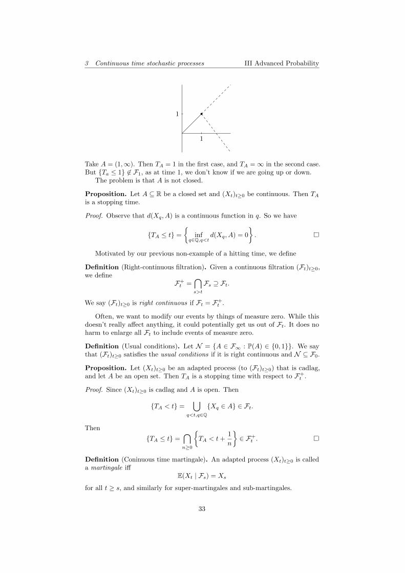
3 Continuous time stochastic processes III Advanced Probability
1
1
Take A = (1,∞). Then TA = 1 in the first case, and TA =∞ in the second case.But Ta ≤ 1 6∈ F1, as at time 1, we don’t know if we are going up or down.
The problem is that A is not closed.
Proposition. Let A ⊆ R be a closed set and (Xt)t≥0 be continuous. Then TAis a stopping time.
Proof. Observe that d(Xq, A) is a continuous function in q. So we have
TA ≤ t =
inf
q∈Q,q<td(Xq, A) = 0
.
Motivated by our previous non-example of a hitting time, we define
Definition (Right-continuous filtration). Given a continuous filtration (Ft)t≥0,we define
F+t =
⋂s>t
Fs ⊇ Ft.
We say (Ft)t≥0 is right continuous if Ft = F+t .
Often, we want to modify our events by things of measure zero. While thisdoesn’t really affect anything, it could potentially get us out of Ft. It does noharm to enlarge all Ft to include events of measure zero.
Definition (Usual conditions). Let N = A ∈ F∞ : P(A) ∈ 0, 1. We saythat (Ft)t≥0 satisfies the usual conditions if it is right continuous and N ⊆ F0.
Proposition. Let (Xt)t≥0 be an adapted process (to (Ft)t≥0) that is cadlag,and let A be an open set. Then TA is a stopping time with respect to F+
t .
Proof. Since (Xt)t≥0 is cadlag and A is open. Then
TA < t =⋃
q<t,q∈QXq ∈ A ∈ Ft.
Then
TA ≤ t =⋂n≥0
TA < t+
1
n
∈ F+
t .
Definition (Coninuous time martingale). An adapted process (Xt)t≥0 is calleda martingale iff
E(Xt | Fs) = Xs
for all t ≥ s, and similarly for super-martingales and sub-martingales.
33
3 Continuous time stochastic processes III Advanced Probability
Note that if t1 ≤ t2 ≤ · · · , then
Xn = Xtn
is a discrete time martingale. Similarly, if t1 ≥ t2 ≥ · · · , and
Xn = Xtn
defines a discrete time backwards martingale. Using this observation, we cannow prove what we already know in the discrete case.
Theorem (Optional stopping theorem). Let (Xt)t≥0 be an adapted cadlagprocess in L1. Then the following are equivalent:
(i) For any bounded stopping time T and any stopping time S, we haveXT ∈ L1 and
E(XT | FS) = XT∧S .
(ii) For any stopping time T , (XTt )t≥0 = (XT∧t)t≥0 is a martingale.
(iii) For any bounded stopping time T , XT ∈ L1 and EXT = EX0.
Proof. We show that (i) ⇒ (ii), and the rest follows from the discrete casesimilarly.
Since T is bounded, assume T ≤ t, and we may wlog assume t ∈ N. Let
Tn = 2−nd2nT e, Sn = 2−nd2nSe.
We have Tn T as n→∞, and so XTn→ XT as n→∞.
Since Tn ≤ t+ 1, by restricting our sequence to Dn, discrete time optionalstopping implies
E(Xt+1 | FTn) = XTn
.
In particular, XTnis uniformly integrable. So it converges in L1. This implies
XT ∈ L1.To show that E(Xt | FS) = XT∧S , we need to show that for any A ∈ FS , we
haveEXt1A = EXS∧T1A.
Since FS ⊆ FSn , we already know that
EXTn1A = lim
n→∞EXSn∧Tn
1A
by discrete time optional stopping, since E(XTn| FSn
) = XTn∧Sn. So taking the
limit n→∞ gives the desired result.
Theorem. Let (Xt)t≥0 be a super-martingale bounded in L1. Then it convergesalmost surely as t→∞ to a random variable X∞ ∈ L1.
Proof. Define Us[a, b, (xt)t≥0] be the number of upcrossings of [a, b] by (xt)t≥0
up to time s, and
U∞[a, b, (xt)t≥0] = lims→∞
Us[a, b, (xt)t≥0].
34
3 Continuous time stochastic processes III Advanced Probability
Then for all s ≥ 0, we have
Us[a, b, (xt)t≥0] = limn→∞
Us[a, b, (x(n)t )t∈Dn ].
By monotone convergence and Doob’s upcrossing lemma, we have
EUs[a, b, (Xt)t≥0] = limn→∞
EUs[a, b, (Xt)t∈Dn] ≤ E(Xs − a)−
b− 1≤ E|Xs|+ a
b− a.
We are then done by taking the supremum over s. Then finish the argument asin the discrete case.
This shows we have pointwise convergence in R ∪ ±∞, and by Fatou’slemma, we know that
E|X∞| = E lim inftn→∞
|Xtn | ≤ lim inftn→∞
E|Xtn | <∞.
So X∞ is finite almost surely.
We shall now state without proof some results we already know for thediscrete case. The proofs are straightforward generalizations of the discreteversion.
Lemma (Maximal inequality). Let (Xt)t≥0 be a cadlag martingale or a non-negative sub-martingale. Then for all t ≥ 0, λ ≥ 0, we have
λP(X∗t ≥ λ) ≤ E|Xt|.
Lemma (Doob’s Lp inequality). Let (Xt)t≥0 be as above. Then
‖X∗t ‖p ≤p
p− 1‖Xt‖p.
Definition (Version). We say a process (Yt)t≥0 is a version of (Xt)t≥0 if for allt, P(Yt = Xt) = 1.
Note that this not the same as saying P(∀t : Yt = Xt) = 1.
Example. Take Xt ≡ 0 for all t and take U be a uniform random variable on[0, 1]. Define
Yt =
1 t = U
0 otherwise.
Then for all t, we have Xt = Yt almost surely. So (Yt) is a version of (Xt).However, Xt is continuous but Yt is not.
Theorem (Regularization of martingales). Let (Xt)t≥0 be a martingale withrespect to (Ft), and suppose Ft satisfies the usual conditions. Then there existsa version (Xt) of (Xt) which is cadlag.
Proof. For all M > 0, define
ΩM0 =
sup
q∈D∩[0,M ]
|Xq| <∞
∩⋂
a<b∈Q
UM [a, b, (Xt)t∈D∩[0,M ]] <∞
35
3 Continuous time stochastic processes III Advanced Probability
Then we see that P(ΩM0 ) = 1 by Doob’s upcrossing lemma. Now define
Xt = lims≥t,s→t,s∈D
Xs1Ωt0.
Then this is Ft measurable because Ft satisfies the usual conditions.Take a sequence tn t. Then (Xtn) is a backwards martingale. So it
converges almost surely in L1 to Xt. But we can write
Xt = E(Xtn | Ft).
Since Xtn → Xt in L1, and Xt is Ft-measurable, we know Xt = Xt almostsurely.
The fact that it is cadlag is an exercise.
Theorem (Lp convergence of martingales). Let (Xt)t≥0 be a cadlag martingale.Then the following are equivalent:
(i) (Xt)t≥0 is bounded in Lp.
(ii) (Xt)t≥0 converges almost surely and in Lp.
(iii) There exists Z ∈ Lp such that Xt = E(Z | Ft) almost surely.
Theorem (L1 convergence of martingales). Let (Xt)t≥0 be a cadlag martingale.Then the folloiwng are equivalent:
(i) (Xt)t≥0 is uniformly integrable.
(ii) (Xt)t≥0 converges almost surely and in L1 to X∞.
(iii) There exists Z ∈ L1 such that E(Z | Ft) = Xt almost surely.
Theorem (Optional stopping theorem). Let (Xt)t≥0 be a uniformly integrablemartingale, and let S, T b e any stopping times. Then
E(XT | Fs) = XS∧T .
36
4 Weak convergence of measures III Advanced Probability
4 Weak convergence of measures
Often, we may want to consider random variables defined on different spaces.Since we cannot directly compare them, a sensible approach would be to usethem to push our measure forward to R, and compare them on R.
Definition (Law). Let X be a random variable on (Ω,F ,P). The law of X isthe probability measure µ on (R,B(R)) defined by
µ(A) = P(X−1(A)).
Example. For x ∈ R, we have the Dirac δ measure
δx(A) = 1x∈A.
This is the law of a random variable that constantly takes the value x.
Now if we have a sequence xn → x, then we would like to say δxn→ δx. In
what sense is this true? Suppose f is continuous. Then∫fdδxn
= f(xn)→ f(x) =
∫fdδx.
So we do have some sort of convergence if we pair it with a continuous function.
Definition (Weak convergence). Let (µn)n≥0, µ be probability measures ona metric space (M,d) with the Borel measure. We say that µn ⇒ µ, or µnconverges weakly to µ if
µn(f)→ µ(f)
for all f bounded and continuous.If (Xn)n≥0 are random variables, then we say (Xn) converges in distribution
if µXn converges weakly.
Note that in general, weak convergence does not say anything about howmeasures of subsets behave.
Example. If xn → x, then δxn → δx weakly. However, if xn 6= x for all n, thenδxn
(x) = 0 but δx(x) = 1. So
δxn(x) 6→ δn(x).
Example. Pick X = [0, 1]. Let µn = 1n
∑nk=1 δ k
n. Then
µn(f) =1
n
n∑k=1
f
(k
n
).
So µn converges to the Lebesgue measure.
Proposition. Let (µn)n≥0 be as above. Then, the following are equivalent:
(i) (µn)n≥0 converges weakly to µ.
(ii) For all open G, we have
lim infn→∞
µn(G) ≥ µ(G).
37
4 Weak convergence of measures III Advanced Probability
(iii) For all closed A, we have
lim supn→∞
µn(A) ≤ µ(A).
(iv) For all A such that µ(∂A) = 0, we have
limn→∞
µn(A) = µ(A)
(v) (when M = R) Fµn(x)→ Fµ(x) for all x at which Fµ is continuous, whereFµ is the distribution function of µ, defined by Fµ(x) = µn((−∞, t]).
Proof.
– (i)⇒ (ii): The idea is to approximate the open set by continuous functions.We know Ac is closed. So we can define
fN (x) = 1 ∧ (N · dist(x,Ac)).
This has the property that for all N > 0, we have
fN ≤ 1A,
and moreover fN 1A as N →∞. Now by definition of weak convergence,
lim infn→∞
µ(A) ≥ lim infn→∞
µn(fN ) = µ(FN )→ µ(A) as N →∞.
– (ii) ⇔ (iii): Take complements.
– (iii) and (ii) ⇒ (iv): Take A such that µ(∂A) = 0. Then
µ(A) = µ(A) = µ(A).
So we know that
lim infn→∞
µn(A) ≥ lim infn→∞
µn(A) ≥ µ(A) = µ(A).
Similarly, we find that
µ(A) ≥ lim supn→∞
µn(A).
So we are done.
– (iv) ⇒ (i): We have
µ(f) =
∫M
f(x) dµ(x)
=
∫M
∫ ∞0
1f(x)≥t dt dµ(x)
=
∫ ∞0
µ(f ≥ t) dt.
Since f is continuous, ∂f ≤ t ⊆ f = t. Now there can be onlycountably many t’s such that µ(f = t) > 0. So replacing µ by limn→∞ µnonly changes the integrand at countably many places, hence doesn’t affectthe integral. So we conclude using bounded convergence theorem.
38
4 Weak convergence of measures III Advanced Probability
– (iv) ⇒ (v): Assume t is a continuity point of Fµ. Then we have
µ(∂(−∞, t]) = µ(t) = Fµ(t)− Fµ(t−) = 0.
So µn(∂n(−∞, t])→ µ((−∞, t]), and we are done.
– (v) ⇒ (ii): If A = (a, b), then
µn(A) ≥ Fµn(b′)− Fµn(a′)
for any a ≤ a′ ≤ b′ ≤ b with a′, b′ continuity points of Fµ. So we knowthat
lim infn→∞
µn(A) ≥ Fµ(b′)− Fµ(a′) = µ(a′, b′).
By taking supremum over all such a′, b′, we find that
lim infn→∞
µn(A) ≥ µ(A).
Definition (Tight probability measures). A sequence of probability measures(µn)n≥0 on a metric space (M, e) is tight if for all ε > 0, there exists compactK ⊆M such that
supnµn(M \K) ≤ ε.
Note that this is always satisfied for compact metric spaces.
Theorem (Prokhorov’s theorem). If (µn)n≥0 is a sequence of tight probabilitymeasures, then there is a subsequence (µnk
)k≥0 and a measure µ such thatµnk⇒ µ.
To see how this can fail without the tightness assumption, suppose we definemeasures µn on R by
µn(A) = µ(A ∩ [n, n+ 1]),
where µ is the Lebesgue measure. Then for any bounded set S, we havelimn→∞ µn(S) = 0. Thus, if the weak limit existed, it must be everywhere zero,but this does not give a probability measure.
We shall prove this only in the case M = R. It is not difficult to construct acandidate of what the weak limit should be. Simply use Bolzano–Weierstrass topick a subsequence of the measures such that the distribution functions convergeon the rationals. Then the limit would essentially be what we want. We thenapply tightness to show that this is a genuine distribution.
Proof. Take Q ⊆ R, which is dense and countable. Let x1, x2, . . . be an enumera-tion of Q. Define Fn = Fµn
. By Bolzano–Weierstrass, and some fiddling aroundwith sequences, we can find some Fnk
such that
Fnk(xi)→ yi ≡ F (xi)
as k →∞, for each fixed xi.Since F is non-decreasing on Q, it has left and right limits everywhere. We
extend F to R by taking right limits. This implies F is cadlag.Take x a continuity point of F . Then for each ε > 0, there exists s < x < t
rational such that|F (s)− F (t)| < ε
2.
39
4 Weak convergence of measures III Advanced Probability
Take n large enough such that |Fn(s) − F (s)| < ε4 , and same for t. Then by
monotonicity of F and Fn, we have
|Fn(x)− F (x)| ≤ |F (s)− F (t)|+ |Fn(s)− F (s)|+ |Fn(t)− F (t)| ≤ ε.
It remains to show that F (x) → 1 as x → ∞ and F (x) → 0 as x → −∞. Bytightness, for all ε > 0, there exists N > 0 such that
µn((−∞, N ]) ≤ ε, µn((N,∞) ≤ ε.
This then implies what we want.
We shall end the chapter with an alternative characterization of weak con-vergence, using characteristic functions.
Definition (Characteristic function). Let X be a random variable taking valuesin Rd. The characteristic function of X is the function Rd → C defined by
ϕX(t) = Eei〈t,x〉 =
∫Rd
ei〈t,x〉 dµX(x).
Note that ϕX is continuous by bounded convergence, and ϕX(0) = 1.
Proposition. If ϕX = ϕY , then µX = µY .
Theorem (Levy’s convergence theroem). Let (Xn)n≥0, X be random variablestaking values in Rd. Then the following are equivalent:
(i) µXn ⇒ µX as n→∞.
(ii) ϕXn→ ϕX pointwise.
We will in fact prove a stronger theorem.
Theorem (Levy). Let (Xn)n≥0 be as above, and let ϕXn(t) → ψ(t) for all t.Suppose ψ is continuous at 0 and ψ(0) = 1. Then there exists a random variableX such that ϕX = ψ and µXn
⇒ µX as n→∞.
We will only prove the case d = 1. We first need the following lemma:
Lemma. Let X be a real random variable. Then for all λ > 0,
µX(|x| ≥ λ) ≤ cλ∫ 1/λ
0
(1− ReϕX(t)) dt,
where C = (1− sin 1)−1.
Proof. For M ≥ 1, we have∫ M
0
(1− cos t) dt = M − sinM ≥M(1− sin 1).
By setting M = |x|λ , we have
1|X|≥λ ≤ Cλ
|X|
∫ |X|/λ0
(1− cos t) dt.
40
4 Weak convergence of measures III Advanced Probability
By a change of variables with t 7→ Xt, we have
1|X|≥λ ≤ cλ∫ 1
0
(1− cosXt) dt.
Apply µX , and use the fact that ReϕX(t) = E cos(Xt).
We can now prove Levy’s theorem.
Proof of theorem. It is clear that weak convergence implies convergence in char-acteristic functions.
Now observe that if µn ⇒ µ iff from every subsequence (nk)k≥0, we canchoose a further subsequence (nk`) such that µnk`
⇒ µ as `→∞. Indeed, ⇒ isclear, and suppose µn 6⇒ µ but satisfies the subsequence property. Then we canchoose a bounded and continuous function f such that
µn(f) 6⇒ µ(f).
Then there is a subsequence (nk)k≥0 such that |µnk(f)− µ(f)| > ε. Then there
is no further subsequence that converges.Thus, to show ⇐, we need to prove the existence of subsequential limits
(uniqueness follows from convergence of characteristic functions). It is enough toprove tightness of the whole sequence.
By the mean value theorem, we can choose λ so large that
cλ
∫ 1/λ
0
(1− Reψ(t)) dt <ε
2.
By bounded convergence, we can choose λ so large that
cλ
∫ 1/λ
0
(1− ReϕXn(t)) dt ≤ ε
for all n. Thus, by our previous lemma, we know (µXn)n≥0 is tight. So we are
done.
41
5 Brownian motion III Advanced Probability
5 Brownian motion
Finally, we can begins studying Brownian motion. Brownian motion was firstobserved by the botanist Robert Brown in 1827, when he looked at the randommovement of pollen grains in water. In 1905, Albert Einstein provided the firstmathematical description of this behaviour. In 1923, Norbert Wiener providedthe first rigorous construction of Brownian motion.
5.1 Basic properties of Brownian motion
Definition (Brownian motion). A continuous process (Bt)t≥0 taking values inRd is called a Brownian motion in Rd started at x ∈ Rd if
(i) B0 = x almost surely.
(ii) For all s < t, the increment Bt −Bs ∼ N(0, (t− s)I).
(iii) Increments are independent. More precisely, for all t1 < t2 < · · · < tk, therandom variables
Bt1 , Bt2 −Bt1 , . . . , Btk −Btk−1
are independent.
If B0 = 0, then we call it a standard Brownian motion.
We always assume our Brownian motion is standard.
Theorem (Wiener’s theorem). There exists a Brownian motion on some proba-bility space.
Proof. We first prove existence on [0, 1] and in d = 1. We wish to applyKolmogorov’s criterion.
Recall that Dn are the dyadic numbers. Let (Zd)d∈D be iid N(0, 1) randomvariables on some probability space. We will define a process on Dn inductivelyon n with the required properties. We wlog assume x = 0.
In step 0, we putB0 = 0, B1 = Z1.
Assume that we have already constructed (Bd)d∈Dn−1satisfying the properties.
Take d ∈ Dn \Dn−1, and set
d± = d± 2−n.
These are the two consecutive numbers in Dn−1 such that d− < d < d+. Define
Bd =Bd+ +Bd−
2+
1
2(n+1)/2Zd.
The condition (i) is trivially satisfied. We now have to check the other twoconditions.
Consider
Bd+ −Bd =Bd+ −Bd−
2− 1
2(n+1)/2Zd
Bd −Bd− =Bd+ −Bd−
2︸ ︷︷ ︸N
+1
2(n+1)/2Zd︸ ︷︷ ︸
N ′
.
42
5 Brownian motion III Advanced Probability
Notice that N and N ′ are normal with variance var(N ′) = var(N) = 12n+1 . In
particular, we have
cov(N −N ′, N +N ′) = var(N)− var(N ′) = 0.
So Bd+ −Bd and Bd −Bd− are independent.Now note that the vector of increments of (Bd)d∈Dn between consecutive
numbers in Dn is Gaussian, since after dotting with any vector, we obtain alinear combination of independent Gaussians. Thus, to prove independence, itsuffice to prove that pairwise correlation vanishes.
We already proved this for the case of increments between Bd and Bd± , andthis is the only case that is tricky, since they both involve the same Zd. Theother cases are straightforward, and are left as an exercise for the reader.
Inductively, we can construct (Bd)d∈D, satisfying (i), (ii) and (iii). Note thatfor all s, t ∈ D, we have
E|Bt −Bs|p = |t− s|p/2E|N |p
for N ∼ N(0, 1). Since E|N |p <∞ for all p, by Kolmogorov’s criterion, we canextend (Bd)d∈D to (Bt)t∈[0,1]. In fact, this is α-Holder continuous for all α < 1
2 .Since this is a continuous process and satisfies the desired properties on
a dense set, it remains to show that the properties are preserved by takingcontinuous limits.
Take 0 ≤ t1 < t2 < · · · < tm ≤ 1, and 0 ≤ tn1 < tn2 < · · · < tnm ≤ 1 such thattni ∈ Dn and tni → ti as n→∞ and i = 1, . . .m.
We now apply Levy’s convergence theorem. Recall that if X is a randomvariable in Rd and X ∼ N(0,Σ), then
ϕX(u) = exp
(−1
2uTΣu
).
Since (Bt)t∈[0,1] is continuous, we have
ϕ(Btn2−Btn1
,...,Btnm−Bn
tm−1)(u) = exp
(−1
2uTΣu
)= exp
(−1
2
m−1∑i=1
(tni+1 − tni )u2i
).
We know this converges, as n→∞, to exp(− 1
2
∑m−1i=1 (ti+1 − ti)u2
i
).
By Levy’s convergence theorem, the law of (Bt2 −Bt1 , Bt3 −Bt2 , . . . , Btn −Btm−1
) is Gaussian with the right covariance. This implies that (ii) and (iii)hold on [0, 1].
To extend the time to [0,∞), we define independent Brownian motions(Bit)t∈[0,1],i∈N and define
Bt =
btc−1∑i=0
Bi1 +Bbtct−btc
To extend to Rd, take the product of d many independent one-dimensionalBrownian motions.
43
5 Brownian motion III Advanced Probability
Lemma. Brownian motion is a Gaussian process, i.e. for any 0 ≤ t1 < t2 <· · · < tm ≤ 1, the vector (Bt1 , Bt2 , . . . , Btn) is Gaussian with covariance
cov(Bt1 , Bt2) = t1 ∧ t2.
Proof. We know (Bt1 , Bt2 − Bt1 , . . . , Btm − Btm−1) is Gaussian. Thus, the
sequence (Bt1 , . . . , Btm) is the image under a linear isomorphism, so it is Gaussian.To compute covariance, for s ≤ t, we have
cov(Bs, Bt) = EBsBt = EBsBT − EB2s + EB2
s = EBs(Bt −Bs) + EB2s = s.
Proposition (Invariance properties). Let (Bt)t≥0 be a standard Brownianmotion in Rd.
(i) If U is an orthogonal matrix, then (UBt)t≥0 is a standard Brownian motion.
(ii) Brownian scaling : If a > 0, then (a−1/2Bat)t≥0 is a standard Brownianmotion. This is known as a random fractal property .
(iii) (Simple) Markov property : For all s ≥ 0, the sequence (Bt+s −Bs)t≥0 is astandard Brownian motion, independent of (FBs ).
(iv) Time inversion: Define a process
Xt =
0 t = 0
tB1/t t > 0.
Then (Xt)t≥0 is a standard Brownian motion.
Proof. Only (iv) requires proof. It is enough to prove that Xt is continuous andhas the right finite-dimensional distributions. We haves
(Xt1 , . . . , Xtm) = (t1B1/t1 , . . . , tmB1/tm).
The right-hand side is the image of (B1/t1 , . . . , B1/tm) under a linear isomorphism.So it is Gaussian. If s ≤ t, then the covariance is
cov(sBs, tBt) = st cov(B1/s, B1/t) = st
(1
s∧ 1
t
)= s = s ∧ t.
Continuity is obvious for t > 0. To prove continuity at 0, we already proved that(Xq)q>0,q∈Q has the same law (as a process) as Brownian motion. By continuityof Xt for positive t, we have
P(
limq∈Q+,q→0
Xq = 0
)= P
(lim
q∈Q+,q→0Bq = 0
)= 1B
by continuity of B.
Using the natural filtration, we have
Theorem. For all s ≥ t, the process (Bt+s −Bs)t≥0 is independent of F+s .
44
5 Brownian motion III Advanced Probability
Proof. Take a sequence sn → s such that sn > s for all n. By continuity,
Bt+s −Bs = limn→∞
Bt+sn −Bsn
almost surely. Now each of Bt+sn −Bsn is independent of F+s , and hence so is
the limit.
Theorem (Blumenthal’s 0-1 law). The σ-algebra F+0 is trivial, i.e. if A ∈ F+
0 ,then P(A) ∈ 0, 1.
Proof. Apply our previous theorem. Take A ∈ F+0 . Then A ∈ σ(Bs : s ≥ 0). So
A is independent of itself.
Proposition.
(i) If d = 1, then
1 = P(inft ≥ 0 : Bt > 0 = 0)
= P(inft ≥ 0 : Bt < 0 = 0)
= P(inft > 0 : Bt = 0 = 0)
(ii) For any d ≥ 1, we have
limt→∞
Btt
= 0
almost surely.
(iii) If we defineSt = sup
0≤s≤tBt, It = inf
0≤s≤tBt,
then S∞ =∞ and I∞ = −∞ almost surely.
(iv) If A is open an Rd, then the cone of A is CA = tx : x ∈ A, t > 0. Theninft ≥ 0 : Bt ∈ CA = 0 almost surely.
Thus, Brownian motion is pretty chaotic.
Proof.
(i) It suffices to prove the first equality. Note that the event inft ≥ 0 : Bk >0 = 0 is trivial. Moreover, for any finite t, the probability that Bt > 0 is12 . Then take a sequence tn such that tn → 0, and apply Fatou to concludethat the probability is positive.
(ii) Follows from the previous one since tB1/t is a Brownian motion.
(iii) By scale invariance, because S∞ = aS∞ for all a > 0.
(iv) Same as (i).
Theorem (Strong Markov property). Let (Bt)t≥0 be a standard Brownianmotion in Rd, and let T be an almost-surely finite stopping time with respect to(F+
t )t≥0. Then
Bt = BT+t −BTis a standard Brownian motion with respect to (F+
T+t)t≥0 that is independent of
F+T .
45
5 Brownian motion III Advanced Probability
Proof. Let Tn = 2−nd2nT e. We first prove the statement for Tn. We let
B(k)t = Bt+k/2n −Bk/2n
This is then a standard Browninan motion independent of F+k/2n by the simple
Markov property. LetB∗(t) = Bt+Tn −BTn .
Let A be the σ-algebra on C = C([0,∞),Rd), and A ∈ A. Let E ∈ F+Tn
. Theclaim that B∗ is a standard Brownian motion independent of E can be conciselycaptured in the equality
P(B∗ ∈ A ∩ E) = P(B ∈ A)P(E). (†)
Taking E = Ω tells us B∗ and B have the same law, and then taking general Etells us B∗ is independent of F+
Tn.
It is a straightforward computation to prove (†). Indeed, we have
P(B∗ ∈ A ∩ E) =
∞∑k=0
P(B(k) ∈ A ∩ E ∩
Tn =
k
2n
)Since E ∈ F+
Tn, we know E ∩ Tn = k/2n ∈ F+
k/2n . So by the simple Markov
property, this is equal to
=
∞∑k=0
P(B(k) ∈ A)P(E ∩
Tn =
k
2n
).
But we know Bk is a standard Brownian motion. So this is equal to
=
∞∑b=0
P(B ∈ A)P(E ∩
Tn =
k
2n
)= P(B ∈ A)P(E).
So we are done.Now as n→∞, the increments of B∗ converge almost surely to the increments
of B, since B is continuous and Tn T almost surely. But B∗ all have the samedistribution, and almost sure convergence implies convergence in distribution.So B is a standard Brownian motion. Being independent of F+
T is clear.
We know that we can reset our process any time we like, and we also knowthat we have a bunch of invariance properties. We can combine these to provesome nice results.
Theorem (Reflection principle). Let (Bt)T≥0 and T be as above. Then the
reflected process (Bt)t≥0 defined by
Bt = Bt1t<T + (2BT −Bt)1t≥T
is a standard Brownian motion.
Of course, the fact that we are reflecting is not important. We can apply anyoperation that preserves the law. This theorem is “obvious”, but we can be abit more careful in writing down a proof.
46
5 Brownian motion III Advanced Probability
Proof. By the strong Markov property, we know
BTt = BT+t −BT
and −BTt are standard Brownian motions independent of F+T . This implies that
the pairs of random variables
P1 = ((Bt)0≤t≤T , (Bt)Tt≥0), P2 = ((Bt)0≤t≤T , (−Bt)Tt≥0)
taking values in C × C have the same law on C × C with the product σ-algebra.Define the concatenation map ψT (X,Y ) : C × C → C by
ψT (X,Y ) = Xt1t<T + (XT + Yt−T )1t≥T .
Assuming Y0 = 0, the resulting process is continuous.Notice that ψT is a measurable map, which we can prove by approximations
of T by discrete stopping times. We then conclude that ψT (P1) has the samelaw as ψT (P2).
Corollary. Let (Bt)T≥0 be a standard Brownian motion in d = 1. Let b > 0and a ≤ b. Let
St = sup0≤s≤t
Bt.
ThenP(St ≥ b, Bt ≤ a) = P(Bt ≥ 2b− a).
Proof. Consider the stopping time T given by the first hitting time of b. SinceS∞ =∞, we know T is finite almost surely. Let (Bt)t≥0 be the reflected process.Then
St ≥ b, Bt ≤ a = Bt ≥ 2b− a.
Corollary. The law of St is equal to the law of |Bt|.
Proof. Apply the previous process with b = a to get
P(St ≥ a) = P(St ≥ a,Bt < a) + P(St ≥ a,Bt ≥ a)
= P(Bt ≥ a) + P(Bt ≥ a)
= P(Bt ≤ a) + P(Bt ≥ a)
= P(|Bt| ≥ a).
Proposition. Let d = 1 and (Bt)t≥0 be a standard Brownian motion. Thenthe following processes are (F+
t )t≥0 martingales:
(i) (Bt)t≥0
(ii) (B2t − t)t≥0
(iii)(
exp(uBt − u2t
2
))t≥0
for u ∈ R.
Proof.
(i) Using the fact that Bt −Bs is independent of F+s , we know
E(Bt −Bs | F+s ) = E(Bt −Bs) = 0.
47
5 Brownian motion III Advanced Probability
(ii) We have
E(B2t − t | F+
s ) = E((Bt −Bs)2 | Fs)− E(B2s | F+
s ) + 2E(BtBs | F+s )− t
We know Bt −Bs is independent of F+s , and so the first term is equal to
var(Bt −Bs) = (t− s), and we can simply to get
= (t− s)−B2s + 2B2
s − t= B2
s − s.
(iii) Similar.
5.2 Harmonic functions and Brownian motion
Recall that a Markov chain plus a harmonic function gave us a martingale. Weshall derive similar results here.
Definition (Domain). A domain is an open connected set D ⊆ Rd.
Definition (Harmonic function). A function u : D → R is called harmonic if
∆f =
d∑i=1
∂2f
∂x2i
= 0.
There is also an alternative characterization of harmonic functions thatinvolves integrals instead of derivatives.
Lemma. Let u : D → R be measurable and locally bounded. Then the followingare equivalent:
(i) u is twice continuously differentiable and ∆u = 0.
(ii) For any x ∈ D and r > 0 such that B(x, r) ⊆ D, we have
u(x) =1
Vol(B(x, r))
∫B(x,r)
u(y) dy
(iii) For any x ∈ D and r > 0 such that B(x, r) ⊆ D, we have
u(x) =1
Area(∂B(x, r))
∫∂B(x,r)
u(y) dy.
The latter two properties are known as the mean value property .
Proof. IA Vector Calculus.
Theorem. Let (Bt)t≥0 be a standard Brownian motion in Rd, and u : Rd → Rbe harmonic such that
E|u(x+Bt)| <∞
for any x ∈ Rd and t ≥ 0. Then the process (u(Bt))t≥0 is a martingale withrespect to (F+
t )t≥0.
To prove this, we need to prove a side lemma:
48
5 Brownian motion III Advanced Probability
Lemma. If X and Y are independent random variables in Rd, and X is G-measurable. If f : Rd × Rd → R is such that f(X,Y ) is integrable, then
E(f(X,Y ) | G) = Ef(z, Y )|z=X .
Proof. Use Fubini and the fact that µ(X,Y ) = µX ⊗ µY .
Observe that if µ is a probability measure in Rd such that the density of µwith respect to the Lebesgue measure depends only on |x|, then if u is harmonic,the mean value property implies
u(x) =
∫Rd
u(x+ y) dµ(y).
Proof of theorem. Let t ≥ s. Then
E(u(Bt) | F+s ) = E(u(Bs + (Bt −Bs)) | F+
s )
= E(u(z +Bt −Bs))|Z=Bs
= u(z)|z=Bs
= u(Bs).
In fact, the following more general result is true:
Theorem. Let f : Rd → R be twice continuously differentiable with boundedderivatives. Then, the processes (Xt)t≥0 defined by
Xt = f(Bt)−1
2
∫ t
0
∆f(Bs) ds
is a martingale with respect to (F+t )t≥0.
We shall not prove this, but we can justify this as follows: suppose we havea sequence of independent random variables X1, X2, . . ., with
P(Xi = ±1) =1
2.
Let Sn = X1 + · · ·+Xn. Then
E(f(Sn+1) | S1, . . . , Sn)−f(Sn) =1
2(f(Sn−1)+f(Sn+1)−2f(sn)) ≡ 1
2∆f(Sn),
and we see that this is the discretized second derivative. So
f(Sn)− 1
2
n−1∑i=0
∆f(Si)
is a martingale.Now the mean value property of a harmonic function u says if we draw a
sphere B centered at x, then u(x) is the average value of u on B. More generally,if we have a surface S containing x, is it true that u(x) is the average value of uon S in some sense?
49
5 Brownian motion III Advanced Probability
Remarkably, the answer is yes, and the precise result is given by Brownianmotion. Let (Xt)t≥0 be a Brownian motion started at x, and let T be the firsthitting time of S. Then, under certain technical conditions, we have
u(x) = Exu(XT ).
In fact, given some function ϕ defined on the boundary of D, we can set
u(x) = Exϕ(XT ),
and this gives us the (unique) solution to Laplace’s equation with the boundarycondition given by ϕ.
It is in fact not hard to show that the resulting u is harmonic in D, sinceit is almost immediate by construction that u(x) is the average of u on a smallsphere around x. The hard part is to show that u is in fact continuous at theboundary, so that it is a genuine solution to the boundary value problem. Thisis where the technical condition comes in.
First, we quickly establish that solutions to Laplace’s equation are unique.
Definition (Maximum principle). Let u : D → R be continuous and harmonic.Then
(i) If u attains its maximum inside D, then u is constant.
(ii) If D is bounded, then the maximum of u in D is attained at ∂D.
Thus, harmonic functions do not have interior maxima unless it is constant.
Proof. Follows from the mean value property of harmonic functions.
Corollary. If u and u′ solve ∆u = ∆u′ = 0, and u and u′ agree on ∂D, thenu = u′.
Proof. u− u′ is also harmonic, and so attains the maximum at the boundary,where it is 0. Similarly, the minimum is attained at the boundary.
The technical condition we impose on D is the following:
Definition (Poincare cone condition). We say a domain D satisfies the Poincarecone condition if for any x ∈ ∂D, there is an open cone C based at X such that
C ∩D ∩B(x, δ) = ∅
for some δ ≥ 0.
Example. If D = R2 \ (0 × R≥0), then D does not satisfy the Poincare conecondition.
And the technical lemma is as follows:
Lemma. Let C be an open cone in Rd based at 0. Then there exists 0 ≤ a < 1such that if |x| ≤ 1
2k , then
Px(T∂B(0,1) < TC) ≤ ak.
50
5 Brownian motion III Advanced Probability
Proof. Picka = sup
|x|≤ 12
Px(T∂B(0,1) < TC) < 1.
We then apply the strong Markov property, and the fact that Brownian motion isscale invariant. We reason as follows — if we start with |x| ≤ 1
2k , we may or may
not hit ∂B(2−k+1) before hitting C. If we don’t, then we are happy. If we are not,then we have reached ∂B(2−k+1). This happens with probability at most a. Nowthat we are at ∂B(2−k+1), the probability of hitting ∂B(2−k+2) before hittingthe cone is at most a again. If we hit ∂B(2−k+3), we again have a probability of≤ a of hitting ∂B(2−k+4), and keep going on. Then by induction, we find thatthe probability of hitting ∂B(0, 1) before hitting the cone is ≤ ak.
The ultimate theorem is then
Theorem. Let D be a bounded domain satisfying the Poincare cone condition,and let ϕ : ∂D → R be continuous. Let
T∂D = inft ≥ 0 : Bt ∈ ∂D.
This is a bounded stopping time. Then the function u : D → R defined by
u(x) = Ex(ϕ(BT∂D)),
where Ex is the expectation if we start at x, is the unique continuous functionsuch that u(x) = ϕ(x) for x ∈ ∂D, and ∆u = 0 for x ∈ D.
Proof. Let τ = T∂B(x,δ) for δ small. Then by the strong Markov property andthe tower law, we have
u(x) = Ex(u(xτ )),
and xτ is uniformly distributed over ∂B(x, δ). So we know u is harmonic in theinterior of D, and in particular is continuous in the interior. It is also clear thatu|∂D = ϕ. So it remains to show that u is continuous up to D.
So let x ∈ ∂D. Since ϕ is continuous, for every ε > 0, there is δ > 0 suchthat if y ∈ ∂D and |y − x| < δ, then |ϕ(y)− ϕ(x)| ≤ ε.
Take z ∈ D such that |z − x| ≤ δ2 . Suppose we start our Brownian motion at
z. If we hit the boundary before we leave the ball, then we are in good shape. Ifnot, then we are sad. But if the second case has small probability, then since ϕis bounded, we can still be fine.
Pick a cone C as in the definition of the Poincare cone condition, and assumewe picked δ small enough that C ∩B(x, δ) ∩D = ∅. Then we have
|u(z)− ϕ(x)| = |Ez(ϕ(BT∂D))− ϕ(x)|
≤ Ez|ϕ(BT∂D− ϕ(x))|
≤ εPz(TB(x,δ) > T∂D) + 2 sup ‖ϕ‖Pz(T∂D > T∂B(x,δ))
≤ ε+ 2‖ϕ‖∞Pz(TB(x,δ) ≤ TC),
and we know the second term → 0 as z → x.
51
5 Brownian motion III Advanced Probability
5.3 Transience and recurrence
Theorem. Let (Bt)t≥0 be a Brownian motion in Rd.
– If d = 1, then (Bt)t≥0 is point recurrent , i.e. for each x, z ∈ R, the sett ≥ 0 : Bt = z is unbounded Px-almost surely.
– If d = 2, then (Bt)t≥0 is neighbourhood recurrent , i.e. for each x ∈ R2 andU ⊆ R2 open, the set t ≥ 0 : Bt ∈ U is unbounded Px-almost surely.However, the process does not visit points, i.e. for all x, z ∈ Rd, we have
PX(Bt = z for some t > 0) = 0.
– If d ≥ 3, then (Bt)t≥0 is transient , i.e. |Bt| → ∞ as t → ∞ Px-almostsurely.
Proof.
– This is trivial, since inft≥0Bt = −∞ and supt≥0Bt = ∞ almost surely,and (Bt)t≥0 is continuous.
– It is enough to prove for x = 0. Let 0 < ε < R <∞ and ϕ ∈ C2b (R2) such
that ϕ(x) = log |x| for ε ≤ |x| ≤ R. It is an easy exercise to check that thisis harmonic inside the annulus. By the theorem we didn’t prove, we know
Mt = ϕ(Bt)−1
2
∫ t
0
∆ϕ(Bs) ds
is a martingale. For λ ≥ 0, let Sλ = inft ≥ 0 : |Bt| = λ. If ε ≤ |x| ≤ R,then H = Sε ∧ SR is PX -almost surely finite. Then MH is a boundedmartingale. By optional stopping, we have
Ex(log |BH |) = log |x|.
But the LHS is
log εP(Sε < SR) + logRP(SR < Sε).
So we find that
Px(Sε < SR) =logR− log |x|logR− log ε
. (∗)
Note that if we let R→∞, then SR →∞ almost surely. Using (∗), thisimplies PX(Sε <∞) = 1, and this does not depend on x. So we are done.
To prove that (Bt)t≥0 does not visit points, let ε → 0 in (∗) and thenR→∞ for x 6= z = 0.
– It is enough to consider the case d = 3. As before, let ϕ ∈ C2b (R3) be such
that
ϕ(x) =1
|x|for ε ≤ x ≤ 2. Then ∆ϕ(x) = 0 for ε ≤ x ≤ R. As before, we get
Px(Sε < SR) =|x|−1 − |R|−1
ε−1 −R−1.
52
5 Brownian motion III Advanced Probability
As R→∞, we have
Px(Sε <∞) =ε
x.
Now letAn = Bt ≥ n for all t ≥ BTn3.
Then
P0(Acn) =1
n2.
So by Borel–Cantelli, we know only finitely of Acn occur almost surely. Soinfinitely many of the An hold. This guarantees our process →∞.
5.4 Donsker’s invariance principle
To end our discussion on Brownian motion, we provide an alternative constructionof Brownian motion, given by Donsker’s invariance principle. Suppose we run anysimple random walk on Zd. We can think of this as a very coarse approximationof a Brownian motion. As we zoom out, the step sizes in the simple randomwalk look smaller and smaller, and if we zoom out sufficiently much, then wemight expect that the result looks like Brownian motion, and indeed it convergesto Brownian motion in the limit.
Theorem (Donsker’s invariance principle). Let (Xn)n≥0 be iid random variableswith mean 0 and variance 1, and set Sn = X1 + · · ·+Xn. Define
St = (1− t)sbtc + tSbtc+1.
where t = t− btc.Define
(S[N ]t )t≥0 = (N−1/2St·N )t∈[0,1].
As (S[N ]t )t∈[0,1] converges in distribution to the law of standard Brownian motion
on [0, 1].
The reader might wonder why we didn’t construct our Brownian motionthis way instead of using Wiener’s theorem. The answer is that our proof ofDonsker’s invariance principle relies on the existence of a Brownian motion! Therelevance is the following theorem:
Theorem (Skorokhod embedding theorem). Let µ be a probability measure onR with mean 0 and variance σ2. Then there exists a probability space (Ω,F ,P)with a filtration (Ft)t≥0 on which there is a standard Brownian motion (Bt)t≥0
and a sequence of stopping times (Tn)n≥0 such that, setting Sn = BTn,
(i) Tn is a random walk with steps of mean σ2
(ii) Sn is a random walk with step distribution µ.
So in some sense, Brownian motion contains all random walks with finitevariance.
The only stopping times we know about are the hitting times of some value.However, if we take Tn to be the hitting time of some fixed value, then BTn
would be a pretty poor attempt at constructing a random walk. Thus, we maytry to come up with the following strategy — construct a probability space
53
5 Brownian motion III Advanced Probability
with a Brownian motion (Bt)t≥0, and an independent iid sequence (Xn)n∈N ofrandom variables with distribution µ. We then take Tn to be the first hittingtime of X1 + · · · + Xn. Then setting Sn = XTn
, property (ii) is by definitionsatisfied. However, (i) will not be satisfied in general. In fact, for any y 6= 0, theexpected first hitting time of y is infinite! The problem is that if, say, y > 0, andwe accidentally strayed off to the negative side, then it could take a long time toreturn.
The solution is to “split” µ into two parts, and construct two random variables(X,Y ) ∈ [0,∞)2, such that if T is T is the first hitting time of (−X,Y ), thenBT has law µ.
Since we are interested in the stopping times T−x and Ty, the followingcomputation will come in handy:
Lemma. Let x, y > 0. Then
P0(T−x < Ty) =y
x+ y, E0T−x ∧ Ty = xy.
Proof sketch. Use optional stopping with (B2t − t)t≥0.
Proof of Skorokhod embedding theorem. Define Borel measures µ± on [0,∞) by
µ±(A) = µ(±A).
Note that these are not probability measures, but we can define a probabilitymeasure ν on [0,∞)2 given by
dν(x, y) = C(x+ y) dµ−(x) dµ+(y)
for some normalizing constant C (this is possible since µ is integrable). This(x+ y) is the same (x+ y) appearing in the denominator of P0(T−x < Ty) = y
x+y .
Then we claim that any (X,Y ) with this distribution will do the job.We first figure out the value of C. Note that since µ has mean 0, we have
C
∫ ∞0
x dµ−(x) = C
∫ ∞0
y dµ+(y).
Thus, we have
1 =
∫C(x+ y) dµ−(x) dµ+(y)
= C
∫x dµ−(x)
∫dµ+(y) + C
∫y dµ+(y)
∫dµ−(x)
= C
∫x dµ−(x)
(∫dµ+(y) +
∫dµ−(x)
)= C
∫x dµ−(x) = C
∫y dµ+(y).
We now set up our notation. Take a probability space (Ω,F ,P) with a stan-dard Brownian motion (Bt)t≥0 and a sequence ((Xn, Yn))n≥0 iid with distributionν and independent of (Bt)t≥0.
DefineF0 = σ((Xn, Yn), n = 1, 2, . . .), Ft = σ(F0,FBt ).
54
5 Brownian motion III Advanced Probability
Define a sequence of stopping times
T0 = 0, Tn+1 = inft ≥ Tn : Bt −BTn∈ −Xn+1, Yn+1.
By the strong Markov property, it suffices to prove that things work in the casen = 1. So for convenience, let T = T1, X = X1, Y = Y1.
To simplify notation, let τ : C([0, 1],R)× [0,∞)2 → [0,∞) be given by
τ(ω, x, y) = inft ≥ 0 : ω(t) ∈ −x, y.
Then we haveT = τ((Bt)t≥0, X, Y ).
To check that this works, i.e. (ii) holds, if A ⊆ [0,∞), then
P(BT ∈ A) =
∫[0,∞)2
∫C([0,∞),R)
1τ(ω,x,y)∈A dµB(ω) dν(x, y).
Using the first part of the previous computation, this is given by∫[0,∞)2
x
x+ y1y∈A C(x+ y) dµ−(x) dµ+(y) = µ+(A).
We can prove a similar result if A ⊆ (−∞, 0). So BT has the right law.To see that T is also well-behaved, we compute
ET =
∫[0,∞)2
∫C([0,1],R)
τ(ω, x, y) dµB(ω) dν(x, y)
=
∫[0,∞)2
xy dν(x, y)
= C
∫[0,∞)2
(x2y + yx2) dµ−(x) dµ+(y)
=
∫[0,∞)
x2 dµ−(x) +
∫[0,∞)
y2 dµ+(y)
= σ2.
The idea of the proof of Donsker’s invariance principle is that in the limit oflarge N , the Tn are roughly regularly spaced, by the law of large numbers, sothis allows us to reverse the above and use the random walk to approximate theBrownian motion.
Proof of Donsker’s invariance principle. Let (Bt)t≥0 be a standard Brownianmotion. Then by Brownian scaling,
(B(N)t )t≥0 = (N1/2Bt/N )t≥0
is a standard Brownian motion.For every N > 0, we let (T
(N)n )n≥0 be a sequence of stopping times as in the
embedding theorem for B(N). We then set
S(N)n = B
(N)
T(N)n
.
55
5 Brownian motion III Advanced Probability
For t not an integer, define S(N)t by linear interpolation. Observe that
((T (N)n )n≥0, S
(N)t ) ∼ ((T (1)
n )n≥0, S(1)t ).
We define
S(N)t = N−1/2S
(N)tN , T (N)
n =T
(N)n
N.
Note that if t = nN , then
S(N)n/N = N−1/2S(N)
n = N−1/2B(N)
T(N)n
= BT
(N)n /N
= BTNn. (∗)
Note that (S(N)t )t≥0 ∼ (S
(N)t )t≥0. We will prove that we have convergence in
probability, i.e. for any δ > 0,
P(
sup0≤t<1
|S(N)t −Bt| > δ
)= P(‖S(N) −B‖∞ > δ)→ 0 as N →∞.
We already know that S and B agree at some times, but the time on S is fixedwhile that on B is random. So what we want to apply is the law of large numbers.By the strong law of large numbers,
limn→∞
1
n|T (1)n − n| → 0 as n→ 0.
This implies that
sup1≤n≤N
1
N|T (1)n − n| → 0 as N →∞.
Note that (T(1)n )n≥0 ∼ (T
(N)n )n≥0, it follows for any δ > 0,
P
(sup
1≤n≤N
∣∣∣∣∣T (N)n
N− n
N
∣∣∣∣∣ ≥ δ)→ 0 as N →∞.
Using (∗) and continuity, for any t ∈ [ nN ,n+1N ], there exists u ∈ [T
(N)n/N , T
(N)(n+1)/N ]
such thatS
(N)t = Bu.
Note that if times are approximated well up to δ, then |t− u| ≤ δ + 1N .
Hence we have
‖S −B‖∞ > ε ≤∣∣∣T (N)
n − n
N
∣∣∣ > δ for some n ≤ N
∪|Bt −Bu| > ε for some t ∈ [0, 1], |t− u| < δ +
1
N
.
The first probability → 0 as n→∞. For the second, we observe that (Bt)T∈[0,1]
has uniformly continuous paths, so for ε > 0, we can find δ > 0 such that thesecond probability is less than ε whenever N > 1
δ (exercise!).
So S(N) → B uniformly in probability, hence converges uniformly in distri-bution.
56
6 Large deviations III Advanced Probability
6 Large deviations
So far, we have been interested in the average or “typical” behaviour of ourprocesses. Now, we are interested in “extreme cases”, i.e. events with smallprobability. In general, our objective is to show that these probabilities tend tozero very quickly.
Let (Xn)n≥0 be a sequence of iid integrable random variables in R and meanvalue EX1 = x and finite variance σ2. We let
Sn = X1 + · · ·+Xn.
By the central limit theorem, we have
P(Sn ≥ nx+√nσa)→ P(Z ≥ a) as n→∞,
where Z ∼ N(0, 1). This implies
P(Sn ≥ an)→ 0
for any a > x. The question is then how fast does this go to zero?There is a very useful lemma in the theory of sequences that tells us this
vanishes exponentially quickly with n. Note that
P(Sm+n ≥ a(m+ n)) ≥ P(Sm ≥ am)P(Sn ≥ an).
So the sequence P(Sn ≥ an) is super-multiplicative. Thus, the sequence
bn = − logP(Sn ≥ an)
is sub-additive.
Lemma (Fekete). If bn is a non-negative sub-additive sequence, then limnbnn
exists.
This implies the rate of decrease is exponential. Can we do better than that,and point out exactly the rate of decrease?
For λ ≥ 0, consider the moment generating function
M(λ) = EeλX1 .
We set ψ(λ) = logM(λ), and the Legendre transform of ψ is
ψ∗(a) = supλ≥0
(aλ− ψ(λ)).
Note that these things may be infinite.
Theorem (Cramer’s theorem). For a > x, we have
limn→∞
1
nlogP(Sn ≥ an) = −ψ∗(a).
Note that we always have
ψ∗(a) = supλ≥0
(aλ− ψ(λ)) ≥ −ψ(0) = 0.
57
6 Large deviations III Advanced Probability
Proof. We first prove an upper bound. For any λ, Markov tells us
P(Sn ≥ an) = P(eλSn ≥ eλan) ≤ e−λanEeλSn
= e−λann∏i=1
EeλXi = e−λanM(λ)n = e−n(λa−ψ(λ)).
Since λ was arbitrary, we can pick λ to maximize λa−ψ(λ), and so by definitionof ψ∗(a), we have P(Sn ≥ an) ≤ e−nψ∗(a). So it follows that
lim sup1
nlogP(Sn ≥ an) ≤ −ψ∗(a).
The lower bound is a bit more involved. One checks that by translating Xi by a,we may assume a = 0, and in particular, x < 0.
So we want to prove that
lim infn
1
nlogP(Sn ≥ 0) ≥ inf
λ≥0ψ(λ).
We consider cases:
– If P(X ≤ 0) = 1, then
P(Sn ≥ 0) = P(Xi = 0 for i = 1, . . . n) = P(X1 = 0)n.
So in fact
lim infn
1
nlogP(Sn ≥ 0) = logP(X1 = 0).
But by monotone convergence, we have
P(X1 = 0) = limλ→∞
EeλX1 .
So we are done.
– Consider the case P(X1 > 0) > 0, but P(X1 ∈ [−K,K]) = 1 for some K.The idea is to modify X1 so that it has mean 0. For µ = µX1
, we define anew distribution by the density
dµθ
dµ(x) =
eθx
M(θ).
We define
g(θ) =
∫x dµθ(x).
We claim that g is continuous for θ ≥ 0. Indeed, by definition,
g(θ) =
∫xeθx dµ(x)∫eθx dµ(x)
,
and both the numerator and denominator are continuous in θ by dominatedconvergence.
Now observe that g(0) = x, and
lim supθ→∞
g(θ) > 0.
58
6 Large deviations III Advanced Probability
So by the intermediate value theorem, we can find some θ0 such thatg(θ0) = 0.
Define µθ0n to be the law of the sum of n iid random variables with law µθ0 .We have
P(Sn ≥ 0) ≥ P(Sn ∈ [0, εn]) ≥ Eeθ0(Sn−εn)1Sn∈[0,εn],
using the fact that on the event Sn ∈ [0, εn], we have eθ0(Sn−εn) ≤ 1. Sowe have
P(Sn ≥ 0) ≥M(θ0)ne−θ0εnµθ0n (Sn ∈ [0, εn]).By the central limit theorem, for each fixed ε, we know
µθ0n (Sn ∈ [0, εn])→ 1
2as n→∞.
So we can write
lim infn
1
nlogP(Sn ≥ 0) ≥ ψ(θ0)− θ0ε.
Then take the limit ε→ 0 to conclude the result.
– Finally, we drop the finiteness assumption, and only assume P(X1 > 0) > 0.We define ν to be the law of X1 condition on the event |X1| ≤ K. Letνn be the law of the sum of n iid random variables with law ν. Define
ψK(λ) = log
∫ K
−Keλx dµ(x)
ψν(λ) = log
∫ ∞−∞
eλx dν(x) = ψK(λ)− logµ(|X| ≤ K).
Note that for K large enough,∫x dν(x) < 0. So we can use the previous
case. By definition of ν, we have
µn([0,∞)) ≥ ν([0,∞))µ(|X| ≤ K)n.
So we have
lim infn
1
nlogµ([0,∞)) ≥ logµ(|X| ≤ K) + lim inf log νn([0,∞))
≥ logµ(|X| ≤ K) + inf ψν(λ)
= infλψK(λ)
= ψλK .
Since ψK increases as K increases to infinity, this increases to some J wehave
lim infn
1
nlogµn([0,∞)) ≥ J . (†)
Since ψK(λ) are continuous, λ : ψK(λ) ≤ J is non-empty, compact andnested in K. By Cantor’s theorem, we can find
λ0 ∈⋂K
λ : ψK(λ) ≤ J.
So the RHS of (†) satisfies
J ≥ supKψK(λ0) = ψ(λ0) ≥ inf
λψ(λ).
59
Index III Advanced Probability
Index
C([0,∞),R), 29C([0,∞),R), 29D([0,∞),R), 29L1(E), 6Lp inequality, 21, 35M(λ), 57U [a, b, (xn), 18Un[a, b, (xn)], 18XT , 15∆, 48B, 4B(E), 4FT , 16F∞, 31σ-field, 4σ-algebra, 4
Borel, 4countably generated, 26product, 6trivial, 24
mE , 4mE+, 4
adapted process, 14almost everywhere, 5atom, 26
backwards filtration, 24backwards martingale, 24Blumenthal’s 0-1 law, 45Borel σ-algebra, 4Brownian motion, 42Brownian scaling, 44
cadlag function, 29cadlag stochastic process, 29characteristic function, 40continuous stochastic process, 29continuous time filtration, 31continuous time martingale, 33continuous time stochastic process,
29continuous time sub-martingale, 33continuous time super-martingale,
33convergence in distribution, 37countably generated σ-algebra, 26
Cramer’s theorem, 57
Dirac δ measure, 37discrete stochastic process, 14distribution
finite-dimensional, 30distribution function, 38domain, 48dominated convergence theorem, 6,
11Doob’s Lp inequality, 21, 35Doob’s upcrossing lemma, 19dyadic numbers, 30
events, 6
Fatou’s lemma, 5, 11Fekete’s lemma, 57filtration, 14
backwards, 24continuous time, 31natural, 14right continuous, 33
finite-dimensional distribution, 30Fubini’s theorem, 6
harmonic function, 27, 48hitting time, 32
increment, 42integrable function, 6integrable process, 14integral, 5
Jensen’s inequality, 11
Kolmogorov 0-1 law, 24Kolmogorov’s criterion, 30
Levy’s convergence theorem, 40Laplacian operator, 48law, 37Legendre transform, 57
Markov chain, 27Markov property, 44martingale, 14
continuous time, 33martingale convergence theorem
60
Index III Advanced Probability
L1, 22, 36Lp, 21, 36almost sure, 18
maximal inequality, 20, 35maximum principle, 50mean value property, 48measurable function, 4measurable space, 4measure, 4
product, 6measure space, 4moment generating function, 57
natural filtration, 14neighbourhood recurrent, 52
optional stopping theorem, 16, 34
Poincare cone condition, 50point recurrent, 52product σ-algebra, 6product measure, 6Prokhorov’s theorem, 39
Radon–Nikodym derivative, 26Radon–Nikodym theorem, 26random fractal property, 44random variables, 6realization, 6reflection principle, 46regularization, 35right continuous filtration, 33
simple function, 5Skorokhod embedding theorem, 53standard Brownian motion, 42stochastic process, 29
adapted, 14cadlag, 29continuous, 29discrete, 14integrable, 14
stopped process, 15stopping time, 15, 32
continuous time, 32strong Markov property, 45sub-martingale, 14
continuous time, 33super-martingale, 14
continuous time, 33
tail σ-algebra, 24tight probability measures, 39Tonelli’s theorem, 6tower property, 11transient, 52transition matrix, 27trivial σ-algebra, 24
upcrossing, 18usual conditions, 33
version, 5, 35
weak convergence, 37Wiener’s theorem, 42
61