
Exceptional Lie Groups, Commutators, and Commutative Homology Rings
Part IB — Groups, Rings and Modules
Based on lectures by O. Randal-WilliamsNotes taken by Dexter Chua
Lent 2016
These notes are not endorsed by the lecturers, and I have modified them (oftensignificantly) after lectures. They are nowhere near accurate representations of what
was actually lectured, and in particular, all errors are almost surely mine.
GroupsBasic concepts of group theory recalled from Part IA Groups. Normal subgroups,quotient groups and isomorphism theorems. Permutation groups. Groups acting onsets, permutation representations. Conjugacy classes, centralizers and normalizers.The centre of a group. Elementary properties of finite p-groups. Examples of finitelinear groups and groups arising from geometry. Simplicity of An.
Sylow subgroups and Sylow theorems. Applications, groups of small order. [8]
RingsDefinition and examples of rings (commutative, with 1). Ideals, homomorphisms,quotient rings, isomorphism theorems. Prime and maximal ideals. Fields. Thecharacteristic of a field. Field of fractions of an integral domain.
Factorization in rings; units, primes and irreducibles. Unique factorization in principalideal domains, and in polynomial rings. Gauss’ Lemma and Eisenstein’s irreducibilitycriterion.
Rings Z[α] of algebraic integers as subsets of C and quotients of Z[x]. Examples ofEuclidean domains and uniqueness and non-uniqueness of factorization. Factorizationin the ring of Gaussian integers; representation of integers as sums of two squares.
Ideals in polynomial rings. Hilbert basis theorem. [10]
Modules
Definitions, examples of vector spaces, abelian groups and vector spaces with an
endomorphism. Sub-modules, homomorphisms, quotient modules and direct sums.
Equivalence of matrices, canonical form. Structure of finitely generated modules over
Euclidean domains, applications to abelian groups and Jordan normal form. [6]
1
Contents IB Groups, Rings and Modules
Contents
0 Introduction 3
1 Groups 41.1 Basic concepts . . . . . . . . . . . . . . . . . . . . . . . . . . . . 41.2 Normal subgroups, quotients, homomorphisms, isomorphisms . . 61.3 Actions of permutations . . . . . . . . . . . . . . . . . . . . . . . 121.4 Conjugacy, centralizers and normalizers . . . . . . . . . . . . . . 171.5 Finite p-groups . . . . . . . . . . . . . . . . . . . . . . . . . . . . 201.6 Finite abelian groups . . . . . . . . . . . . . . . . . . . . . . . . . 221.7 Sylow theorems . . . . . . . . . . . . . . . . . . . . . . . . . . . . 23
2 Rings 282.1 Definitions and examples . . . . . . . . . . . . . . . . . . . . . . . 282.2 Homomorphisms, ideals, quotients and isomorphisms . . . . . . . 312.3 Integral domains, field of factions, maximal and prime ideals . . 392.4 Factorization in integral domains . . . . . . . . . . . . . . . . . . 432.5 Factorization in polynomial rings . . . . . . . . . . . . . . . . . . 512.6 Gaussian integers . . . . . . . . . . . . . . . . . . . . . . . . . . . 572.7 Algebraic integers . . . . . . . . . . . . . . . . . . . . . . . . . . . 602.8 Noetherian rings . . . . . . . . . . . . . . . . . . . . . . . . . . . 62
3 Modules 663.1 Definitions and examples . . . . . . . . . . . . . . . . . . . . . . . 663.2 Direct sums and free modules . . . . . . . . . . . . . . . . . . . . 713.3 Matrices over Euclidean domains . . . . . . . . . . . . . . . . . . 753.4 Modules over F[X] and normal forms for matrices . . . . . . . . . 863.5 Conjugacy of matrices* . . . . . . . . . . . . . . . . . . . . . . . 91
Index 95
2
0 Introduction IB Groups, Rings and Modules
0 Introduction
The course is naturally divided into three sections — Groups, Rings, and Modules.In IA Groups, we learnt about some basic properties of groups, and studied
several interesting groups in depth. In the first part of this course, we willfurther develop some general theory of groups. In particular, we will prove twomore isomorphism theorems of groups. While we will not find these theoremsparticularly useful in this course, we will be able to formulate analogous theoremsfor other algebraic structures such as rings and modules, as we will later find inthe course.
In the next part of the course, we will study rings. These are things thatbehave somewhat like Z, where we can add, subtract, multiply but not (necessar-ily) divide. While Z has many nice properties, these are not necessarily availablein arbitrary rings. Hence we will classify rings into different types, depending onhow many properties of Z they inherit. We can then try to reconstruct certain IANumbers and Sets results in these rings, such as unique factorization of numbersinto primes and Bezout’s theorem.
Finally, we move on to modules. The definition of a module is very similarto that of a vector space, except that instead of allowing scalar multiplicationby elements of a field, we have scalar multiplication by elements of a ring. Itturns out modules are completely unlike vector spaces, and can have much morecomplicated structures. Perhaps because of this richness, many things turn outto be modules. Using module theory, we will be able to prove certain importanttheorems such as the classification of finite abelian groups and the Jordan normalform theorem.
3
1 Groups IB Groups, Rings and Modules
1 Groups
1.1 Basic concepts
We will begin by quickly recapping some definitions and results from IA Groups.
Definition (Group). A group is a triple (G, · , e), where G is a set, · : G×G→ Gis a function and e ∈ G is an element such that
(i) For all a, b, c ∈ G, we have (a · b) · c = a · (b · c). (associativity)
(ii) For all a ∈ G, we have a · e = e · a = a. (identity)
(iii) For all a ∈ G, there exists a−1 ∈ G such that a · a−1 = a−1 · a = e.(inverse)
Some people add a stupid axiom that says g · h ∈ G for all g, h ∈ G, but thisis already implied by saying · is a function to G. You can write that down aswell, and no one will say you are stupid. But they might secretly think so.
Lemma. The inverse of an element is unique.
Proof. Let a−1, b be inverses of a. Then
b = b · e = b · a · a−1 = e · a−1 = a−1.
Definition (Subgroup). If (G, · , e) is a group and H ⊆ G is a subset, it is asubgroup if
(i) e ∈ H,
(ii) a, b ∈ H implies a · b ∈ H,
(iii) · : H ×H → H makes (H, · , e) a group.
We write H ≤ G if H is a subgroup of G.
Note that the last condition in some sense encompasses the first two, but weneed the first two conditions to hold before the last statement makes sense at all.
Lemma. H ⊆ G is a subgroup if H is non-empty and for any h1, h2 ∈ H, wehave h1h
−12 ∈ H.
Definition (Abelian group). A group G is abelian if a · b = b · a for all a, b ∈ G.
Example. We have the following familiar examples of groups
(i) (Z,+, 0), (Q,+, 0), (R,+, 0), (C,+, 0).
(ii) We also have groups of symmetries:
(a) The symmetric group Sn is the collection of all permutations of1, 2, · · · , n.
(b) The dihedral group D2n is the symmetries of a regular n-gon.
(c) The group GLn(R) is the group of invertible n × n real matrices,which also is the group of invertible R-linear maps from the vectorspace Rn to itself.
4
1 Groups IB Groups, Rings and Modules
(iii) The alternating group An ≤ Sn.
(iv) The cyclic group Cn ≤ D2n.
(v) The special linear group SLn(R) ≤ GLn(R), the subgroup of matrices ofdeterminant 1.
(vi) The Klein-four group C2 × C2.
(vii) The quaternions Q8 = ±1,±i,±j,±k with ij = k, ji = −k, i2 = j2 =k2 = −1, (−1)2 = 1.
With groups and subgroups, we can talk about cosets.
Definition (Coset). If H ≤ G, g ∈ G, the left coset gH is the set
gH = x ∈ G : x = g · h for some h ∈ H.
For example, since H is a subgroup, we know e ∈ H. So for any g ∈ G, wemust have g ∈ gH.
The collection of H-cosets in G forms a partition of G, and furthermore,all H-cosets gH are in bijection with H itself, via h 7→ gh. An immediateconsequence is
Theorem (Lagrange’s theorem). Let G be a finite group, and H ≤ G. Then
|G| = |H||G : H|,
where |G : H| is the number of H-cosets in G.
We can do exactly the same thing with right cosets and get the sameconclusion.
We have implicitly used the following notation:
Definition (Order of group). The order of a group is the number of elementsin G, written |G|.
Instead of order of the group, we can ask what the order of an element is.
Definition (Order of element). The order of an element g ∈ G is the smallestpositive n such that gn = e. If there is no such n, we say g has infinite order.
We write ord(g) = n.
A basic lemma is as follows:
Lemma. If G is a finite group and g ∈ G has order n, then n | |G|.
Proof. Consider the following subset:
H = e, g, g2, · · · , gn−1.
This is a subgroup of G, because it is non-empty and grg−s = gr−s is on the list(we might have to add n to the power of g to make it positive, but this is finesince gn = e). Moreover, there are no repeats in the list: if gi = gj , with wlogi ≥ j, then gi−j = e. So i− j < n. By definition of n, we must have i− j = 0,i.e. i = j.
Hence Lagrange’s theorem tells us n = |H| | |G|.
5
1 Groups IB Groups, Rings and Modules
1.2 Normal subgroups, quotients, homomorphisms, iso-morphisms
We all (hopefully) recall what the definition of a normal subgroup is. However,instead of just stating the definition and proving things about it, we can try tomotivate the definition, and see how one could naturally come up with it.
Let H ≤ G be a subgroup. The objective is to try to make the collection ofcosets
G/H = gH : g ∈ Ginto a group.
Before we do that, we quickly come up with a criterion for when two cosetsgH and g′H are equal. Notice that if gH = g′H, then g ∈ g′H. So g = g′ · h forsome h. In other words, (g′)−1 · g = h ∈ H. So if two elements represent thesame coset, their difference is in H. The argument is also reversible. Hence twoelements g, g′ represent the same H-coset if and only if (g′)−1g ∈ H.
Suppose we try to make the set G/H = gH : g ∈ G into a group, by theobvious formula
(g1H) · (g2H) = g1g2H.
However, this doesn’t necessarily make sense. If we take a different representativefor the same coset, we want to make sure it gives the same answer.
If g2H = g′2H, then we know g′2 = g2 · h for some h ∈ H. So
(g1H) · (g′2H) = g1g′2H = g1g2hH = g1g2H = (g1H) · (g2H).
So all is good.What if we change g1? If g1H = g′1H, then g′1 = g1 · h for some h ∈ H. So
(g′1H) · (g2H) = g′1g2H = g1hg2H.
Now we are stuck. We would really want the equality
g1hg2H = g1g2H
to hold. This requires(g1g2)−1g1hg2 ∈ H.
This is equivalent tog−1
2 hg2 ∈ H.So for G/H to actually be a group under this operation, we must have, for anyh ∈ H and g ∈ G, the property g−1hg ∈ H to hold.
This is not necessarily true for an arbitrary H. Those nice ones that satisfythis property are known as normal subgroups.
Definition (Normal subgroup). A subgroup H ≤ G is normal if for any h ∈ Hand g ∈ G, we have g−1hg ∈ H. We write H CG.
This allows us to make the following definition:
Definition (Quotient group). If HCG is a normal subgroup, then the set G/Hof left H-cosets forms a group with multiplication
(g1H) · (g2H) = g1g2H.
with identity eH = H. This is known as the quotient group.
6
1 Groups IB Groups, Rings and Modules
This is indeed a group. Normality was defined such that this is well-defined.Multiplication is associative since multiplication in G is associative. The inverseof gH is g−1H, and eH is easily seen to be the identity.
So far, we’ve just been looking at groups themselves. We would also like toknow how groups interact with each other. In other words, we want to studyfunctions between groups. However, we don’t allow arbitrary functions, sincegroups have some structure, and we would like the functions to respect the groupstructures. These nice functions are known as homomorphisms.
Definition (Homomorphism). If (G, · , eG) and (H, ∗, eH) are groups, a functionφ : G→ H is a homomorphism if φ(eG) = eH , and for g, g′ ∈ G, we have
φ(g · g′) = φ(g) ∗ φ(g′).
If we think carefully, φ(eG) = eH can be derived from the second condition,but it doesn’t hurt to put it in as well.
Lemma. If φ : G→ H is a homomorphism, then
φ(g−1) = φ(g)−1.
Proof. We compute φ(g · g−1) in two ways. On the one hand, we have
φ(g · g−1) = φ(e) = e.
On the other hand, we have
φ(g · g−1) = φ(g) ∗ φ(g−1).
By the uniqueness of inverse, we must have
φ(g−1) = φ(g)−1.
Given any homomorphism, we can build two groups out of it:
Definition (Kernel). The kernel of a homomorphism φ : G→ H is
ker(φ) = g ∈ G : φ(g) = e.
Definition (Image). The image of a homomorphism φ : G→ H is
im(φ) = h ∈ H : h = φ(g) for some g ∈ G.
Lemma. For a homomorphism φ : G → H, the kernel ker(φ) is a normalsubgroup, and the image im(φ) is a subgroup of H.
Proof. There is only one possible way we can prove this.To see ker(φ) is a subgroup, let g, h ∈ kerφ. Then
φ(g · h−1) = φ(g) ∗ φ(h)−1 = e ∗ e−1 = e.
So gh−1 ∈ kerφ. Also, φ(e) = e. So ker(φ) is non-empty. So it is a subgroup.To show it is normal, let g ∈ ker(φ). Let x ∈ G. We want to show
x−1gx ∈ ker(φ). We have
φ(x−1gx) = φ(x−1) ∗ φ(g) ∗ φ(x) = φ(x−1) ∗ φ(x) = φ(x−1x) = φ(e) = e.
7
1 Groups IB Groups, Rings and Modules
So x−1gx ∈ ker(φ). So ker(φ) is normal.Also, if φ(g), φ(h) ∈ im(φ), then
φ(g) ∗ φ(h)−1 = φ(gh−1) ∈ im(φ).
Also, e ∈ im(φ). So im(φ) is non-empty. So im(φ) is a subgroup.
Definition (Isomorphism). An isomorphism is a homomorphism that is also abijection.
Definition (Isomorphic group). Two groups G and H are isomorphic if thereis an isomorphism between them. We write G ∼= H.
Usually, we identify two isomorphic groups as being “the same”, and do notdistinguish isomorphic groups.
It is an exercise to show the following:
Lemma. If φ is an isomorphism, then the inverse φ−1 is also an isomorphism.
When studying groups, it is often helpful to break the group apart into smallergroups, which are hopefully easier to study. We will have three isomorphismtheorems to do so. These isomorphism theorems tell us what happens when wetake quotients of different things. Then if a miracle happens, we can patch whatwe know about the quotients together to get information about the big group.Even if miracles do not happen, these are useful tools to have.
The first isomorphism relates the kernel to the image.
Theorem (First isomorphism theorem). Let φ : G→ H be a homomorphism.Then ker(φ)CG and
G
ker(φ)∼= im(φ).
Proof. We have already proved that ker(φ) is a normal subgroup. We nowhave to construct a homomorphism f : G/ ker(φ) → im(φ), and prove it is anisomorphism.
Define our function as follows:
f :G
ker(φ)→ im(φ)
g ker(φ) 7→ φ(g).
We first tackle the obvious problem that this might not be well-defined, since weare picking a representative for the coset. If g ker(φ) = g′ ker(φ), then we knowg−1 · g′ ∈ ker(φ). So φ(g−1 · g′) = e. So we know
e = φ(g−1 · g′) = φ(g)−1 ∗ φ(g′).
Multiplying the whole thing by φ(g) gives φ(g) = φ(g′). Hence this function iswell-defined.
Next we show it is a homomorphism. To see f is a homomorphism, we have
f(g ker(φ) · g′ ker(φ)) = f(gg′ ker(φ))
= φ(gg′)
= φ(g) ∗ φ(g′)
= f(g ker(φ)) ∗ f(g′ ker(φ)).
8
1 Groups IB Groups, Rings and Modules
So f is a homomorphism. Finally, we show it is a bijection.To show it is surjective, let h ∈ im(φ). Then h = φ(g) for some g. So
h = f(g ker(φ)) is in the image of f .To show injectivity, suppose f(g ker(φ)) = f(g′ ker(φ)). So φ(g) = φ(g′). So
φ(g−1 · g′) = e. Hence g−1 · g′ ∈ ker(φ), and hence g ker(φ) = g′ ker(φ). Sodone.
Before we move on to further isomorphism theorems, we see how we can usethese to identify two groups which are not obviously the same.
Example. Consider a homomorphism φ : C → C \ 0 given by z 7→ ez. Wealso know that
ez+w = ezew.
This means φ is a homomorphism if we think of it as φ : (C,+)→ (C \ 0,×).What is the image of this homomorphism? The existence of log shows that
φ is surjective. So imφ = C \ 0. What about the kernel? It is given by
ker(φ) = z ∈ C : ez = 1 = 2πiZ,
i.e. the set of all integer multiples of 2πi. The conclusion is that
(C/(2πiZ),+) ∼= (C \ 0,×).
The second isomorphism theorem is a slightly more complicated theorem.
Theorem (Second isomorphism theorem). Let H ≤ G and K C G. ThenHK = h · k : h ∈ H, k ∈ K is a subgroup of G, and H ∩K CH. Moreover,
HK
K∼=
H
H ∩K.
Proof. Let hk, h′k′ ∈ HK. Then
h′k′(hk)−1 = h′k′k−1h−1 = (h′h−1)(hk′k−1h−1).
The first term is in H, while the second term is k′k−1 ∈ K conjugated byh, which also has to be in K be normality. So this is something in H timessomething in K, and hence in HK. HK also contains e, and is hence a group.
To show H ∩KCH, consider x ∈ H ∩K and h ∈ H. Consider h−1xh. Sincex ∈ K, the normality of K implies h−1xh ∈ K. Also, since x, h ∈ H, closureimplies h−1xh ∈ H. So h−1xh ∈ H ∩K. So H ∩K CH.
Now we can start to prove the second isomorphism theorem. To do so, weapply the first isomorphism theorem to it. Define
φ : H → G/K
h 7→ hK
This is easily seen to be a homomorphism. We apply the first isomorphismtheorem to this homomorphism. The image is all K-cosets represented bysomething in H, i.e.
im(φ) =HK
K.
9
1 Groups IB Groups, Rings and Modules
Then the kernel of φ is
ker(φ) = h ∈ H : hK = eK = h ∈ H : h ∈ K = H ∩K.
So the first isomorphism theorem says
H
H ∩K∼=HK
K.
Notice we did more work than we really had to. We could have started bywriting down φ and checked it is a homomorphism. Then since H ∩K is itskernel, it has to be a normal subgroup.
Before we move on to the third isomorphism theorem, we notice that ifK CG, then there is a bijection between subgroups of G/K and subgroups of Gcontaining K, given by
subgroups of G/K ←→ subgroups of G which contain K
X ≤ G
K−→ g ∈ G : gK ∈ X
L
K≤ G
K←− K C L ≤ G.
This specializes to the bijection of normal subgroups:
normal subgroups of G/K ←→ normal subgroups of G which contain K
using the same bijection.It is an elementary exercise to show that these are inverses of each other.
This correspondence will be useful in later times.
Theorem (Third isomorphism theorem). Let K ≤ L ≤ G be normal subgroupsof G. Then
G
K
/ LK∼=G
L.
Proof. Define the homomorphism
φ : G/K → G/L
gK 7→ gL
As always, we have to check this is well-defined. If gK = g′K, then g−1g′ ∈K ⊆ L. So gL = g′L. This is also a homomorphism since
φ(gK · g′K) = φ(gg′K) = gg′L = (gL) · (g′L) = φ(gK) · φ(g′K).
This clearly is surjective, since any coset gL is the image φ(gK). So the imageis G/L. The kernel is then
ker(φ) = gK : gL = L = gK : g ∈ L =L
K.
So the conclusion follows by the first isomorphism theorem.
The general idea of these theorems is to take a group, find a normal subgroup,and then quotient it out. Then hopefully the normal subgroup and the quotientgroup will be simpler. However, this doesn’t always work.
10
1 Groups IB Groups, Rings and Modules
Definition (Simple group). A (non-trivial) group G is simple if it has no normalsubgroups except e and G.
In general, simple groups are complicated. However, if we only look at abeliangroups, then life is simpler. Note that by commutativity, the normality conditionis always trivially satisfied. So any subgroup is normal. Hence an abelian groupcan be simple only if it has no non-trivial subgroups at all.
Lemma. An abelian group is simple if and only if it is isomorphic to the cyclicgroup Cp for some prime number p.
Proof. By Lagrange’s theorem, any subgroup of Cp has order dividing |Cp| = p.Hence if p is prime, then it has no such divisors, and any subgroup must haveorder 1 or p, i.e. it is either e or Cp itself. Hence in particular any normalsubgroup must be e or Cp. So it is simple.
Now suppose G is abelian and simple. Let e 6= g ∈ G be a non-trivial element,and consider H = · · · , g−2, g−1, e, g, g2, · · · . Since G is abelian, conjugationdoes nothing, and every subgroup is normal. So H is a normal subgroup. As Gis simple, H = e or H = G. Since it contains g 6= e, it is non-trivial. So wemust have H = G. So G is cyclic.
If G is infinite cyclic, then it is isomorphic to Z. But Z is not simple, since2ZC Z. So G is a finite cyclic group, i.e. G ∼= Cm for some finite m.
If n | m, then gm/n generates a subgroup of G of order n. So this is a normalsubgroup. Therefore n must be m or 1. Hence G cannot be simple unless m hasno divisors except 1 and m, i.e. m is a prime.
One reason why simple groups are important is the following:
Theorem. Let G be any finite group. Then there are subgroups
G = H1 BH2 BH3 BH4 B · · ·BHn = e.
such that Hi/Hi+1 is simple.
Note that here we only claim that Hi+1 is normal in Hi. This does not saythat, say, H3 is a normal subgroup of H1.
Proof. If G is simple, let H2 = e. Then we are done.If G is not simple, let H2 be a maximal proper normal subgroup of G. We
now claim that G/H2 is simple.If G/H2 is not simple, it contains a proper non-trivial normal subgroup
L C G/H2 such that L 6= e, G/H2. However, there is a correspondencebetween normal subgroups of G/H2 and normal subgroups of G containing H2.So L must be K/H2 for some K CG such that K ≥ H2. Moreover, since L isnon-trivial and not G/H2, we know K is not G or H2. So K is a larger normalsubgroup. Contradiction.
So we have found an H2CG such that G/H2 is simple. Iterating this processon H2 gives the desired result. Note that this process eventually stops, asHi+1 < Hi, and hence |Hi+1| < |Hi|, and all these numbers are finite.
11
1 Groups IB Groups, Rings and Modules
1.3 Actions of permutations
When we first motivated groups, we wanted to use them to represent somecollection of “symmetries”. Roughly, a symmetry of a set X is a permutationof X, i.e. a bijection X → X that leaves some nice properties unchanged. Forexample, a symmetry of a square is a permutation of the vertices that leaves theoverall shape of the square unchanged.
Instead of just picking some nice permutations, we can consider the group ofall permutations. We call this the symmetric group.
Definition (Symmetric group). The symmetric group Sn is the group of allpermutations of 1, · · · , n, i.e. the set of all bijections of this set with itself.
A convenient way of writing permutations is to use the disjoint cycle notation,such as writing (1 2 3)(4 5)(6) for the permutation that maps
1 7→ 2 4 7→ 5
2 7→ 3 5 7→ 4
3 7→ 1 6 7→ 6.
Unfortunately, the convention for writing permutations is weird. Since permuta-tions are bijections, and hence functions, they are multiplied the wrong way, i.e.f g means first apply g, then apply f . In particular, (1 2 3)(3 4) requires firstapplying the second permutation, then the first, and is in fact (1 2 3 4).
We know that any permutation is a product of transpositions. Hence wemake the following definition.
Definition (Even and odd permutation). A permutation σ ∈ Sn is even if itcan be written as a product of evenly many transpositions; odd otherwise.
In IA Groups, we spent a lot of time proving this is well-defined, and we arenot doing that again (note that this definition by itself is well-defined — if apermutation can be both written as an even number of transposition and an oddnumber of transposition, the definition says it is even. However, this is not whatwe really want, since we cannot immediately conclude that, say, (1 2) is odd).
This allows us to define the homomorphism:
sgn : Sn → (±1,×)
σ 7→
+1 σ is even
−1 σ is odd
Definition (Alternating group). The alternating group An ≤ Sn is the subgroupof even permutations, i.e. An is the kernel of sgn.
This immediately tells us An C Sn, and we can immediately work out itsindex, since
SnAn∼= im(sgn) = ±1,
unless n = 1. So An has index 2.More generally, for a set X, we can define its symmetric group as follows:
Definition (Symmetric group of X). Let X be a set. We write Sym(X) for thegroup of all permutations of X.
12
1 Groups IB Groups, Rings and Modules
However, we don’t always want the whole symmetric group. Sometimes, wejust want some subgroups of symmetric groups, as in our initial motivation. Sowe make the following definition.
Definition (Permutation group). A group G is called a permutation group if itis a subgroup of Sym(X) for some X, i.e. it is given by some, but not necessarilyall, permutations of some set.
We say G is a permutation group of order n if in addition |X| = n.
This is not really a too interesting definition, since, as we will soon see, everygroup is (isomorphic to) a permutation group. However, in some cases, thinkingof a group as a permutation group of some object gives us better intuition onwhat the group is about.
Example. Sn and An are obviously permutation groups. Also, the dihedralgroup D2n is a permutation group of order n, viewing it as a permutation of thevertices of a regular n-gon.
We would next want to recover the idea of a group being a “permutation”.If G ≤ Sym(X), then each g ∈ G should be able to give us a permutation of X,in a way that is consistent with the group structure. We say the group G actson X. In general, we make the following definition:
Definition (Group action). An action of a group (G, · ) on a set X is a function
∗ : G×X → X
such that
(i) g1 ∗ (g2 ∗ x) = (g1 · g2) ∗ x for all g1, g2 ∈ G and x ∈ X.
(ii) e ∗ x = x for all x ∈ X.
There is another way of defining group actions, which is arguably a betterway of thinking about group actions.
Lemma. An action of G on X is equivalent to a homomorphism φ : G →Sym(X).
Note that the statement by itself is useless, since it doesn’t tell us how totranslate between the homomorphism and a group action. The important partis the proof.
Proof. Let ∗ : G×X → X be an action. Define φ : G→ Sym(X) by sending gto the function φ(g) = (g ∗ · : X → X). This is indeed a permutation — g−1 ∗ ·is an inverse since
φ(g−1)(φ(g)(x)) = g−1 ∗ (g ∗ x) = (g−1 · g) ∗ x = e ∗ x = x,
and a similar argument shows φ(g)φ(g−1) = idX . So φ is at least a well-definedfunction.
To show it is a homomorphism, just note that
φ(g1)(φ(g2)(x)) = g1 ∗ (g2 ∗ x) = (g1 · g2) ∗ x = φ(g1 · g2)(x).
13
1 Groups IB Groups, Rings and Modules
Since this is true for all x ∈ X, we know φ(g1) φ(g2) = φ(g1 · g2). Also,φ(e)(x) = e ∗ x = x. So φ(e) is indeed the identity. Hence φ is a homomorphism.
We now do the same thing backwards. Given a homomorphism φ : G →Sym(X), define a function by g ∗x = φ(g)(x). We now check it is indeed a groupaction. Using the definition of a homomorphism, we know
(i) g1 ∗ (g2 ∗ x) = φ(g1)(φ(g2)(x)) = (φ(g1) φ(g2))(x) = φ(g1 · g2)(x) =(g1 · g2) ∗ x.
(ii) e ∗ x = φ(e)(x) = idX(x) = x.
So this homomorphism gives a group action. These two operations are clearly in-verses to each other. So group actions of G on X are the same as homomorphismsG→ Sym(X).
Definition (Permutation representation). A permutation representation of agroup G is a homomorphism G→ Sym(X).
We have thus shown that a permutation representation is the same as agroup action.
The good thing about thinking of group actions as homomorphisms is thatwe can use all we know about homomorphisms on them.
Notation. For an action of G on X given by φ : G → Sym(X), we writeGX = im(φ) and GX = ker(φ).
The first isomorphism theorem immediately gives
Proposition. GX CG and G/GX ∼= GX .
In particular, if GX = e is trivial, then G ∼= GX ≤ Sym(X).
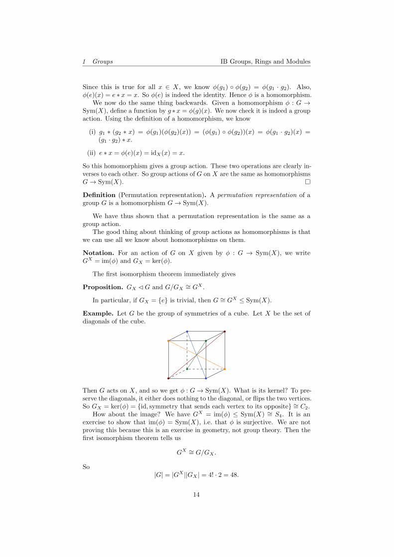
Example. Let G be the group of symmetries of a cube. Let X be the set ofdiagonals of the cube.
Then G acts on X, and so we get φ : G→ Sym(X). What is its kernel? To pre-serve the diagonals, it either does nothing to the diagonal, or flips the two vertices.So GX = ker(φ) = id, symmetry that sends each vertex to its opposite ∼= C2.
How about the image? We have GX = im(φ) ≤ Sym(X) ∼= S4. It is anexercise to show that im(φ) = Sym(X), i.e. that φ is surjective. We are notproving this because this is an exercise in geometry, not group theory. Then thefirst isomorphism theorem tells us
GX ∼= G/GX .
So|G| = |GX ||GX | = 4! · 2 = 48.
14
1 Groups IB Groups, Rings and Modules
This is an example of how we can use group actions to count elements in agroup.
Example (Cayley’s theorem). For any group G, we have an action of G on Gitself via
g ∗ g1 = gg1.
It is trivial to check this is indeed an action. This gives a group homomorphismφ : G → Sym(G). What is its kernel? If g ∈ ker(φ), then it acts trivially onevery element. In particular, it acts trivially on the identity. So g ∗ e = e, whichmeans g = e. So ker(φ) = e. By the first isomorphism theorem, we get
G ∼= G/e ∼= imφ ≤ Sym(G).
So we know every group is (isomorphic to) a subgroup of a symmetric group.
Example. Let H be a subgroup of G, and X = G/H be the set of left cosetsof H. We let G act on X via
g ∗ g1H = gg1H.
It is easy to check this is well-defined and is indeed a group action. So we getφ : G→ Sym(X).
Now consider GX = ker(φ). If g ∈ GX , then for every g1 ∈ G, we haveg ∗ g1H = g1H. This means g−1
1 gg1 ∈ H. In other words, we have
g ∈ g1Hg−11 .
This has to happen for all g1 ∈ G. So
GX ⊆⋂g1∈G
g1Hg−11 .
This argument is completely reversible — if g ∈⋂g1∈G g1Hg
−11 , then for each
g1 ∈ G, we knowg−1
1 gg1 ∈ H,
and hencegg1H = g1H.
Sog ∗ g1H = g1H
So g ∈ GX . Hence we indeed have equality:
ker(φ) = GX =⋂g1∈G
g1Hg−11 .
Since this is a kernel, this is a normal subgroup of G, and is contained in H.Starting with an arbitrary subgroup H, this allows us to generate a normalsubgroup, and this is indeed the biggest normal subgroup of G that is containedin H, if we stare at it long enough.
We can use this to prove the following theorem.
15
1 Groups IB Groups, Rings and Modules
Theorem. Let G be a finite group, and H ≤ G a subgroup of index n. Thenthere is a normal subgroup K CG with K ≤ H such that G/K is isomorphic toa subgroup of Sn. Hence |G/K| | n! and |G/K| ≥ n.
Proof. We apply the previous example, giving φ : G→ Sym(G/H), and let Kbe the kernel of this homomorphism. We have already shown that K ≤ H. Thenthe first isomorphism theorem gives
G/K ∼= imφ ≤ Sym(G/H) ∼= Sn.
Then by Lagrange’s theorem, we know |G/K| | |Sn| = n!, and we also have|G/K| ≥ |G/H| = n.
Corollary. Let G be a non-abelian simple group. Let H ≤ G be a propersubgroup of index n. Then G is isomorphic to a subgroup of An. Moreover, wemust have n ≥ 5, i.e. G cannot have a subgroup of index less than 5.
Proof. The action of G on X = G/H gives a homomorphism φ : G→ Sym(X).Then ker(φ) C G. Since G is simple, ker(φ) is either G or e. We first showthat it cannot be G. If ker(φ) = G, then every element of G acts trivially onX = G/H. But if g ∈ G \H, which exists since the index of H is not 1, theng ∗H = gH 6= H. So g does not act trivially. So the kernel cannot be the wholeof G. Hence ker(φ) = e.
Thus by the first isomorphism theorem, we get
G ∼= im(φ) ≤ Sym(X) ∼= Sn.
We now need to show that G is in fact a subgroup of An.We know An C Sn. So im(φ) ∩An C im(φ) ∼= G. As G is simple, im(φ) ∩An
is either e or G = im(φ). We want to show that the second thing happens,i.e. the intersection is not the trivial group. We use the second isomorphismtheorem. If im(φ) ∩An = e, then
im(φ) ∼=im(φ)
im(φ) ∩An∼=
im(φ)AnAn
≤ SnAn∼= C2.
So G ∼= im(φ) is a subgroup of C2, i.e. either e or C2 itself. Neither of these arenon-abelian. So this cannot be the case. So we must have im(φ) ∩An = im(φ),i.e. im(φ) ≤ An.
The last part follows from the fact that S1, S2, S3, S4 have no non-abeliansimple subgroups, which you can check by going to a quiet room and listing outall their subgroups.
Let’s recall some old definitions from IA Groups.
Definition (Orbit). If G acts on a set X, the orbit of x ∈ X is
G · x = g ∗ x ∈ X : g ∈ G.
Definition (Stabilizer). If G acts on a set X, the stabilizer of x ∈ X is
Gx = g ∈ G : g ∗ x = x.
The main theorem about these concepts is the orbit-stabilizer theorem.
16
1 Groups IB Groups, Rings and Modules
Theorem (Orbit-stabilizer theorem). Let G act on X. Then for any x ∈ X,there is a bijection between G · x and G/Gx, given by g · x↔ g ·Gx.
In particular, if G is finite, it follows that
|G| = |Gx||G · x|.
It takes some work to show this is well-defined and a bijection, but you’vedone it in IA Groups. In IA Groups, you probably learnt the second statementinstead, but this result is more generally true for infinite groups.
1.4 Conjugacy, centralizers and normalizers
We have seen that every group acts on itself by multiplying on the left. A groupG can also act on itself in a different way, by conjugation:
g ∗ g1 = gg1g−1.
Let φ : G→ Sym(G) be the associated permutation representation. We know,by definition, that φ(g) is a bijection from G to G as sets. However, here G isnot an arbitrary set, but is a group. A natural question to ask is whether φ(g)is a homomorphism or not. Indeed, we have
φ(g)(g1 · g2) = gg1g2g−1 = (gg1g
−1)(gg2g−1) = φ(g)(g1)φ(g)(g2).
So φ(g) is a homomorphism from G to G. Since φ(g) is bijective (as in anygroup action), it is in fact an isomorphism.
Thus, for any group G, there are many isomorphisms from G to itself, onefor every g ∈ G, and can be obtained from a group action of G on itself.
We can, of course, take the collection of all isomorphisms of G, and form anew group out of it.
Definition (Automorphism group). The automorphism group of G is
Aut(G) = f : G→ G : f is a group isomorphism.
This is a group under composition, with the identity map as the identity.
This is a subgroup of Sym(G), and the homomorphism φ : G→ Sym(G) byconjugation lands in Aut(G).
This is pretty fun — we can use this to cook up some more groups, by takinga group and looking at its automorphism group.
We can also take a group, take its automorphism group, and then take itsautomorphism group again, and do it again, and see if this process stabilizes, orbecomes periodic, or something. This is left as an exercise for the reader.
Definition (Conjugacy class). The conjugacy class of g ∈ G is
cclG(g) = hgh−1 : h ∈ G,
i.e. the orbit of g ∈ G under the conjugation action.
Definition (Centralizer). The centralizer of g ∈ G is
CG(g) = h ∈ G : hgh−1 = g,
i.e. the stabilizer of g under the conjugation action. This is alternatively the setof all h ∈ G that commute with g.
17
1 Groups IB Groups, Rings and Modules
Definition (Center). The center of a group G is
Z(G) = h ∈ G : hgh−1 = g for all g ∈ G =⋂g∈G
CG(g) = ker(φ).
These are the elements of the group that commute with everything else.By the orbit-stabilizer theorem, for each x ∈ G, we obtain a bijection
ccl(x)↔ G/CG(x).
Proposition. Let G be a finite group. Then
| ccl(x)| = |G : CG(x)| = |G|/|CG(x)|.
In particular, the size of each conjugacy class divides the order of the group.Another useful notion is the normalizer.
Definition (Normalizer). Let H ≤ G. The normalizer of H in G is
NG(H) = g ∈ G : g−1Hg = H.
Note that we certainly haveH ≤ NG(H). Even better, HCNG(H), essentiallyby definition. This is in fact the biggest subgroup of G in which H is normal.
We are now going to look at conjugacy classes of Sn. Now we recall from IAGroups that permutations in Sn are conjugate if and only if they have the samecycle type when written as a product of disjoint cycles. We can think of thecycle types as partitions of n. For example, the partition 2, 2, 1 of 5 correspondsto the conjugacy class of (1 2)(3 4)(5). So the conjugacy classes of Sn are exactlythe partitions of n.
We will use this fact in the proof of the following theorem:
Theorem. The alternating groups An are simple for n ≥ 5 (also for n = 1, 2, 3).
The cases in brackets follow from a direct check since A1∼= A2
∼= e andA3∼= C3, all of which are simple. We can also check manually that A4 has
non-trivial normal subgroups, and hence not simple.Recall we also proved that A5 is simple in IA Groups by brute force — we
listed all its conjugacy classes, and see they cannot be put together to make anormal subgroup. This obviously cannot be easily generalized to higher valuesof n. Hence we need to prove this with a different approach.
Proof. We start with the following claim:
Claim. An is generated by 3-cycles.
As any element of An is a product of evenly-many transpositions, it sufficesto show that every product of two transpositions is also a product of 3-cycles.
There are three possible cases: let a, b, c, d be distinct. Then
(i) (a b)(a b) = e.
(ii) (a b)(b c) = (a b c).
(iii) (a b)(c d) = (a c b)(a c d).
So we have shown that every possible product of two transpositions is a productof three-cycles.
18
1 Groups IB Groups, Rings and Modules
Claim. Let H CAn. If H contains a 3-cycle, then we H = An.
We show that if H contains a 3-cycle, then every 3-cycle is in H. Then weare done since An is generated by 3-cycles. For concreteness, suppose we know(a b c) ∈ H, and we want to show (1 2 3) ∈ H.
Since they have the same cycle type, so we have σ ∈ Sn such that (a b c) =σ(1 2 3)σ−1. If σ is even, i.e. σ ∈ An, then we have that (1 2 3) ∈ σ−1Hσ = H,by the normality of H and we are trivially done.
If σ is odd, replace it by σ = σ · (4 5). Here is where we use the fact thatn ≥ 5 (we will use it again later). Then we have
σ(1 2 3)σ−1 = σ(4 5)(1 2 3)(4 5)σ−1 = σ(1 2 3)σ−1 = (a b c),
using the fact that (1 2 3) and (4 5) commute. Now σ is even. So (1 2 3) ∈ H asabove.
What we’ve got so far is that if H CAn contains any 3-cycle, then it is An.Finally, we have to show that every normal subgroup must contain at least one3-cycle.
Claim. Let H CAn be non-trivial. Then H contains a 3-cycle.
We separate this into many cases
(i) Suppose H contains an element which can be written in disjoint cyclenotation
σ = (1 2 3 · · · r)τ,
for r ≥ 4. We now let δ = (1 2 3) ∈ An. Then by normality of H, we knowδ−1σδ ∈ H. Then σ−1δ−1σδ ∈ H. Also, we notice that τ does not contain1, 2, 3. So it commutes with δ, and also trivially with (1 2 3 · · · r). Wecan expand this mess to obtain
σ−1δ−1σδ = (r · · · 2 1)(1 3 2)(1 2 3 · · · r)(1 2 3) = (2 3 r),
which is a 3-cycle. So done.
The same argument goes through if σ = (a1 a2 · · · ar)τ for any a1, · · · , an.
(ii) Suppose H contains an element consisting of at least two 3-cycles in disjointcycle notation, say
σ = (1 2 3)(4 5 6)τ
We now let δ = (1 2 4), and again calculate
σ−1δ−1σδ = (1 3 2)(4 6 5)(1 4 2)(1 2 3)(4 5 6)(1 2 4) = (1 2 4 3 6).
This is a 5-cycle, which is necessarily in H. By the previous case, we get a3-cycle in H too, and hence H = An.
(iii) Suppose H contains σ = (1 2 3)τ , with τ a product of 2-cycles (if τ containsanything longer, then it would fit in one of the previous two cases). Thenσ2 = (1 2 3)2 = (1 3 2) is a three-cycle.
19
1 Groups IB Groups, Rings and Modules
(iv) Suppose H contains σ = (1 2)(3 4)τ , where τ is a product of 2-cycles. Wefirst let δ = (1 2 3) and calculate
u = σ−1δ−1σδ = (1 2)(3 4)(1 3 2)(1 2)(3 4)(1 2 3) = (1 4)(2 3),
which is again in u. We landed in the same case, but instead of twotranspositions times a mess, we just have two transpositions, which is nicer.Now let
v = (1 5 2)u(1 2 5) = (1 3)(4 5) ∈ H.
Note that we used n ≥ 5 again. We have yet again landed in the same case.Notice however, that these are not the same transpositions. We multiply
uv = (1 4)(2 3)(1 3)(4 5) = (1 2 3 4 5) ∈ H.
This is then covered by the first case, and we are done.
So done. Phew.
1.5 Finite p-groups
Note that when studying the orders of groups and subgroups, we always talkabout divisibility, since that is what Lagrange’s theorem tells us about. Wenever talk about things like the sum of the orders of two subgroups. When itcomes to divisibility, the simplest case would be when the order is a prime, andwe have done that already. The next best thing we can hope for is that the orderis a power of a prime.
Definition (p-group). A finite group G is a p-group if |G| = pn for some primenumber p and n ≥ 1.
Theorem. If G is a finite p-group, then Z(G) = x ∈ G : xg = gx for all g ∈ Gis non-trivial.
This immediately tells us that for n ≥ 2, a p group is never simple.
Proof. Let G act on itself by conjugation. The orbits of this action (i.e. theconjugacy classes) have order dividing |G| = pn. So it is either a singleton, orits size is divisible by p.
Since the conjugacy classes partitionG, we know the total size of the conjugacyclasses is |G|. In particular,
|G| = number of conjugacy class of size 1
+∑
order of all other conjugacy classes.
We know the second term is divisible by p. Also |G| = pn is divisible by p. Hencethe number of conjugacy classes of size 1 is divisible by p. We know e is aconjugacy class of size 1. So there must be at least p conjugacy classes of size 1.Since the smallest prime number is 2, there is a conjugacy class x 6= e.
But if x is a conjugacy class on its own, then by definition g−1xg = x forall g ∈ G, i.e. xg = gx for all g ∈ G. So x ∈ Z(G). So Z(G) is non-trivial.
20
1 Groups IB Groups, Rings and Modules
The theorem allows us to prove interesting things about p-groups by induction— we can quotient G by Z(G), and get a smaller p-group. One way to do this isvia the below lemma.
Lemma. For any group G, if G/Z(G) is cyclic, then G is abelian.In other words, if G/Z(G) is cyclic, then it is in fact trivial, since the center
of an abelian group is the abelian group itself.
Proof. Let g ∈ Z(G) be a generator of the cyclic group G/Z(G). Hence everycoset of Z(G) is of the form grZ(G). So every element x ∈ G must be of theform grz for z ∈ Z(G) and r ∈ Z. To show G is abelian, let x = gr z be anotherelement, with z ∈ Z(G), r ∈ Z. Note that z and z are in the center, and hencecommute with every element. So we have
xx = grzgr z = grgrzz = grgr zz = gr zgrz = xx.
So they commute. So G is abelian.
This is a general lemma for groups, but is particularly useful when appliedto p groups.
Corollary. If p is prime and |G| = p2, then G is abelian.
Proof. Since Z(G) ≤ G, its order must be 1, p or p2. Since it is not trivial, itcan only be p or p2. If it has order p2, then it is the whole group and the groupis abelian. Otherwise, G/Z(G) has order p2/p = p. But then it must be cyclic,and thus G must be abelian. This is a contradiction. So G is abelian.
Theorem. Let G be a group of order pa, where p is a prime number. Then ithas a subgroup of order pb for any 0 ≤ b ≤ a.
This means there is a subgroup of every conceivable order. This is not truefor general groups. For example, A5 has no subgroup of order 30 or else thatwould be a normal subgroup.
Proof. We induct on a. If a = 1, then e, G give subgroups of order p0 and p1.So done.
Now suppose a > 1, and we want to construct a subgroup of order pb. Ifb = 0, then this is trivial, namely e ≤ G has order 1.
Otherwise, we know Z(G) is non-trivial. So let x 6= e ∈ Z(G). Since
ord(x) | |G|, its order is a power of p. If it in fact has order pc, then xpc−1
hasorder p. So we can suppose, by renaming, that x has order p. We have thusgenerated a subgroup 〈x〉 of order exactly p. Moreover, since x is in the center,〈x〉 commutes with everything in G. So 〈x〉 is in fact a normal subgroup of G.This is the point of choosing it in the center. Therefore G/〈x〉 has order pa−1.
Since this is a strictly smaller group, we can by induction suppose G/〈x〉 hasa subgroup of any order. In particular, it has a subgroup L of order pb−1. Bythe subgroup correspondence, there is some K ≤ G such that L = K/〈x〉 andH CK. But then K has order pb. So done.
21
1 Groups IB Groups, Rings and Modules
1.6 Finite abelian groups
We now move on to a small section, which is small because we will come back toit later, and actually prove what we claim.
It turns out finite abelian groups are very easy to classify. We can just writedown a list of all finite abelian groups. We write down the classification theorem,and then prove it in the last part of the course, where we hit this with a hugesledgehammer.
Theorem (Classification of finite abelian groups). Let G be a finite abeliangroup. Then there exist some d1, · · · , dr such that
G ∼= Cd1 × Cd2 × · · · × Cdr .
Moreover, we can pick di such that di+1 | di for each i, and this expression isunique.
It turns out the best way to prove this is not to think of it as a group, butas a Z-module, which is something we will come to later.
Example. The abelian groups of order 8 are C8, C4 × C2, C2 × C2 × C2.
Sometimes this is not the most useful form of decomposition. To get a nicerdecomposition, we use the following lemma:
Lemma. If n and m are coprime, then Cmn ∼= Cm × Cn.
This is a grown-up version of the Chinese remainder theorem. This is whatthe Chinese remainder theorem really says.
Proof. It suffices to find an element of order nm in Cm×Cn. Then since Cn×Cmhas order nm, it must be cyclic, and hence isomorphic to Cnm.
Let g ∈ Cm have order m; h ∈ Cn have order n, and consider (g, h) ∈ Cm×Cn.Suppose the order of (g, h) is k. Then (g, h)k = (e, e). Hence (gk, hk) = (e, e).So the order of g and h divide k, i.e. m | k and n | k. As m and n are coprime,this means that mn | k.
As k = ord((g, h)) and (g, h) ∈ Cm × Cn is a group of order mn, we musthave k | nm. So k = nm.
Corollary. For any finite abelian group G, we have
G ∼= Cd1 × Cd2 × · · · × Cdr ,
where each di is some prime power.
Proof. From the classification theorem, iteratively apply the previous lemma tobreak each component up into products of prime powers.
As promised, this is short.
22
1 Groups IB Groups, Rings and Modules
1.7 Sylow theorems
We finally get to the big theorem of this part of the course.
Theorem (Sylow theorems). Let G be a finite group of order pa ·m, with p aprime and p - m. Then
(i) The set of Sylow p-subgroups of G, given by
Sylp(G) = P ≤ G : |P | = pa,
is non-empty. In other words, G has a subgroup of of order pa.
(ii) All elements of Sylp(G) are conjugate in G.
(iii) The number of Sylow p-subgroups np = |Sylp(G)| satisfies np ≡ 1 (mod p)and np | |G| (in fact np | m, since p is not a factor of np).
These are sometimes known as Sylow’s first/second/third theorem respec-tively.
We will not prove this just yet. We first look at how we can apply thistheorem. We can use it without knowing how to prove it.
Lemma. If np = 1, then the Sylow p-subgroup is normal in G.
Proof. Let P be the unique Sylow p-subgroup, and let g ∈ G, and considerg−1Pg. Since this is isomorphic to P , we must have |g−1Pg| = pa, i.e. it is alsoa Sylow p-subgroup. Since there is only one, we must have P = g−1Pg. So P isnormal.
Corollary. Let G be a non-abelian simple group. Then |G| | np!2 for every prime
p such that p | |G|.
Proof. The group G acts on Sylp(G) by conjugation. So it gives a permutationrepresentation φ : G → Sym(Sylp(G)) ∼= Snp . We know kerφ C G. But G issimple. So ker(φ) = e or G. We want to show it is not the whole of G.
If we had G = ker(φ), then g−1Pg = P for all g ∈ G. Hence P is a normalsubgroup. As G is simple, either P = e, or P = G. We know P cannot betrivial since p | |G|. But if G = P , then G is a p-group, has a non-trivial center,and hence G is not non-abelian simple. So we must have ker(φ) = e.
Then by the first isomorphism theorem, we know G ∼= imφ ≤ Snp . We haveproved the theorem without the divide-by-two part. To prove the whole result,we need to show that in fact im(φ) ≤ Anp . Consider the following compositionof homomorphisms:
G Snp ±1.φ sgn
If this is surjective, then ker(sgn φ)CG has index 2 (since the index is the sizeof the image), and is not the whole of G. This means G is not simple (the casewhere |G| = C2 is ruled out since it is abelian).
So the kernel must be the whole G, and sgn φ is the trivial map. In otherwords, sgn(φ(g)) = +1. So φ(g) ∈ Anp . So in fact we have
G ∼= im(φ) ≤ Anp .
So we get |G| | np!2 .
23
1 Groups IB Groups, Rings and Modules
Example. Suppose |G| = 1000. Then |G| is not simple. To show this, we needto factorize 1000. We have |G| = 23 · 53. We pick our favorite prime to be p = 5.We know n5
∼= 1 (mod 5), and n5 | 23 = 8. The only number that satisfies thisis n5 = 1. So the Sylow 5-subgroup is normal, and hence G is not normal.
Example. Let |G| = 132 = 22 · 3 · 11. We want to show this is not simple. Sofor a contradiction suppose it is.
We start by looking at p = 11. We know n11 ≡ 1 (mod 11). Also n11 | 12.As G is simple, we must have n11 = 12.
Now look at p = 3. We have n3 = 1 (mod 3) and n3 | 44. The possiblevalues of n3 are 4 and 22.
If n3 = 4, then the corollary says |G| | 4!2 = 12, which is of course nonsense.
So n3 = 22.At this point, we count how many elements of each order there are. This is
particularly useful if p | |G| but p2 - |G|, i.e. the Sylow p-subgroups have order pand hence are cyclic.
As all Sylow 11-subgroups are disjoint, apart from e, we know there are12 · (11− 1) = 120 elements of order 11. We do the same thing with the Sylow3-subgroups. We need 22 · (3 − 1) = 44 elements of order 3. But this is moreelements than the group has. This can’t happen. So G must be simple.
We now get to prove our big theorem. This involves some non-trivial amountof trickery.
Proof of Sylow’s theorem. Let G be a finite group with |G| = pam, and p - m.
(i) We need to show that Sylp(G) 6= ∅, i.e. we need to find some subgroup oforder pa. As always, we find something clever for G to act on. We let
Ω = X subset of G : |X| = pa.
We let G act on Ω by
g ∗ g1, g2, · · · , gpa = gg1, gg2, · · · , ggpa.
Let Σ ≤ Ω be an orbit.
We first note that if g1, · · · , gpa ∈ Σ, then by the definition of an orbit,for every g ∈ G,
gg−11 ∗ g1, · · · , gpa = g, gg−1
1 g2, · · · , gg−11 gpa ∈ Σ.
The important thing is that this set contains g. So for each g, Σ containsa set X which contains g. Since each set X has size pa, we must have
|Σ| ≥ |G|pa
= m.
Suppose |Σ| = m. Then the orbit-stabilizer theorem says the stabilizer H ofany g1, · · · , gpa ∈ Σ has index m, hence |H| = pa, and thus H ∈ Sylp(G).
So we need to show that not every orbit Σ can have size > m. Again, bythe orbit-stabilizer, the size of any orbit divides the order of the group,|G| = pam. So if |Σ| > m, then p | |Σ|. Suppose we can show that p - |Ω|.
24
1 Groups IB Groups, Rings and Modules
Then not every orbit Σ can have size > m, since Ω is the disjoint union ofall the orbits, and thus we are done.
So we have to show p - |Ω|. This is just some basic counting. We have
|Ω| =(|G|pa
)=
(pam
pa
)=
pa−1∏j=0
=pam− jpa − j
.
Now note that the largest power of p dividing pam− j is the largest powerof p dividing j. Similarly, the largest power of p dividing pa − j is also thelargest power of p dividing j. So we have the same power of p on top andbottom for each item in the product, and they cancel. So the result is notdivisible by p.
This proof is not straightforward. We first needed the clever idea of lettingG act on Ω. But then if we are given this set, the obvious thing to dowould be to find something in Ω that is also a group. This is not what wedo. Instead, we find an orbit whose stabilizer is a Sylow p-subgroup.
(ii) We instead prove something stronger: if Q ≤ G is a p-subgroup (i.e.|Q| = pb, for b not necessarily a), and P ≤ G is a Sylow p-subgroup, thenthere is a g ∈ G such that g−1Qg ≤ P . Applying this to the case where Qis another Sylow p-subgroup says there is a g such that g−1Qg ≤ P , butsince g−1Qg has the same size as P , they must be equal.
We let Q act on the set of cosets of G/P via
q ∗ gP = qgP.
We know the orbits of this action have size dividing |Q|, so is either 1 ordivisible by p. But they can’t all be divisible by p, since |G/P | is coprimeto p. So at least one of them have size 1, say gP. In other words, forevery q ∈ Q, we have qgP = gP . This means g−1qg ∈ P . This holds forevery element q ∈ Q. So we have found a g such that g−1Qg ≤ P .
(iii) Finally, we need to show that np ∼= 1 (mod p) and np | |G|, where np =|SylP (G)|.The second part is easier — by Sylow’s second theorem, the action of Gon Sylp(G) by conjugation has one orbit. By the orbit-stabilizer theorem,the size of the orbit, which is |Sylp(G)| = np, divides |G|. This proves thesecond part.
For the first part, let P ∈ SylP (G). Consider the action by conjugationof P on Sylp(G). Again by the orbit-stabilizer theorem, the orbits eachhave size 1 or size divisible by p. But we know there is one orbit of size 1,namely P itself. To show np = |SylP (G)| ∼= 1 (mod p), it is enough toshow there are no other orbits of size 1.
Suppose Q is an orbit of size 1. This means for every p ∈ P , we get
p−1Qp = Q.
In other words, P ≤ NG(Q). Now NG(Q) is itself a group, and wecan look at its Sylow p-subgroups. We know Q ≤ NG(Q) ≤ G. So
25
1 Groups IB Groups, Rings and Modules
pa | |NG(Q)| | pam. So pa is the biggest power of p that divides |NG(Q)|.So Q is a Sylow p-subgroup of NG(Q).
Now we know P ≤ NG(Q) is also a Sylow p-subgroup of NG(Q). By Sylow’ssecond theorem, they must be conjugate in NG(Q). But conjugatinganything in Q by something in NG(Q) does nothing, by definition ofNG(Q). So we must have P = Q. So the only orbit of size 1 is P itself.So done.
This is all the theories of groups we’ve got. In the remaining time, we willlook at some interesting examples of groups.
Example. Let G = GLn(Z/p), i.e. the set of invertible n × n matrices withentries in Z/p, the integers modulo p. Here p is obviously a prime. When we dorings later, we will study this properly.
First of all, we would like to know the size of this group. A matrix A ∈GLn(Z/p) is the same as n linearly independent vectors in the vector space(Z/p)n. We can just work out how many there are. This is not too difficult,when you know how.
We can pick the first vector, which can be anything except zero. So thereare pn − 1 ways of choosing the first vector. Next, we need to pick the secondvector. This can be anything that is not in the span of the first vector, and thisrules out p possibilities. So there are pn − p ways of choosing the second vector.Continuing this chain of thought, we have
|GLn(Z/p)| = (pn − 1)(pn − p)(pn − p2) · · · (pn − pn−1).
What is a Sylow p-subgroup of GLn(Z/p)? We first work out what the order ofthis is. We can factorize that as
|GLn(Z/p)| = (1 · p · p2 · · · · · pn−1)((pn − 1)(pn−1 − 1) · · · (p− 1)).
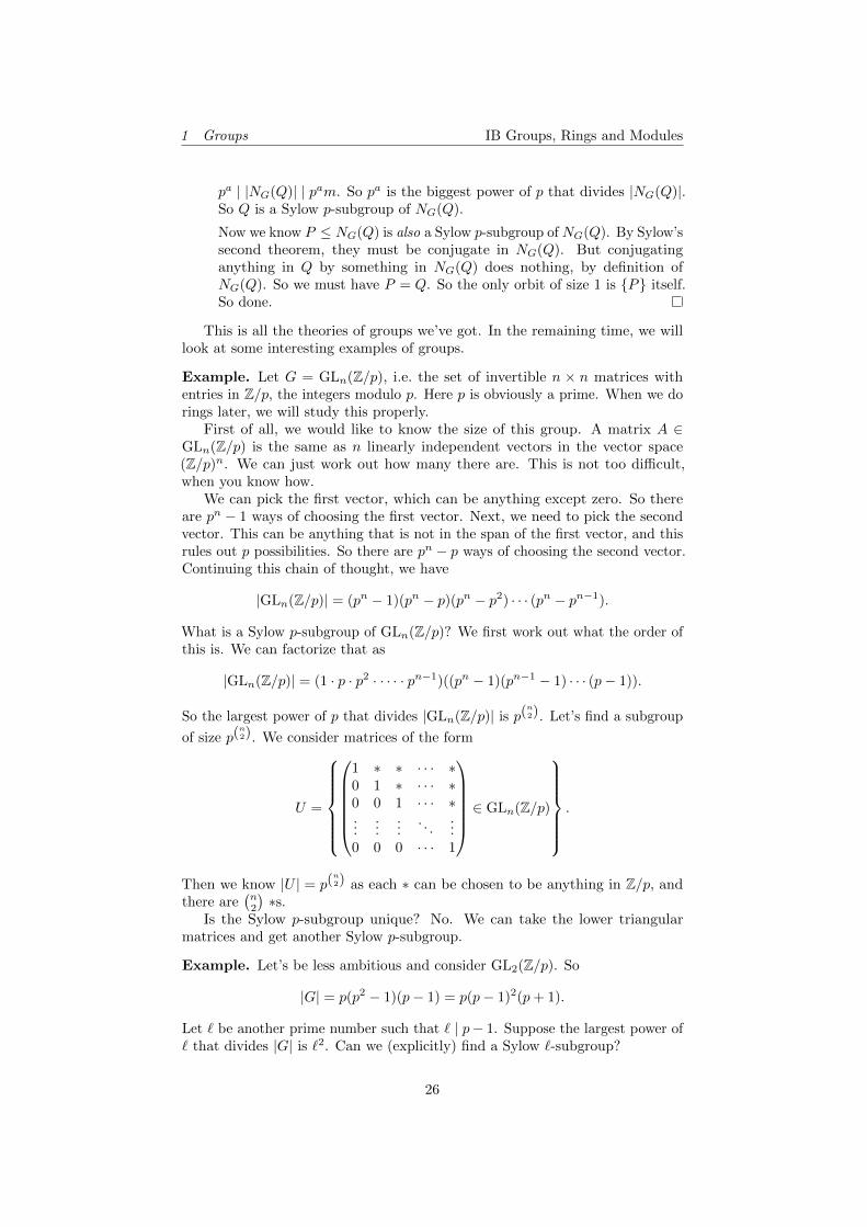
So the largest power of p that divides |GLn(Z/p)| is p(n2). Let’s find a subgroup
of size p(n2). We consider matrices of the form
U =
1 ∗ ∗ · · · ∗0 1 ∗ · · · ∗0 0 1 · · · ∗...
......
. . ....
0 0 0 · · · 1
∈ GLn(Z/p)
.
Then we know |U | = p(n2) as each ∗ can be chosen to be anything in Z/p, and
there are(n2
)∗s.
Is the Sylow p-subgroup unique? No. We can take the lower triangularmatrices and get another Sylow p-subgroup.
Example. Let’s be less ambitious and consider GL2(Z/p). So
|G| = p(p2 − 1)(p− 1) = p(p− 1)2(p+ 1).
Let ` be another prime number such that ` | p− 1. Suppose the largest power of` that divides |G| is `2. Can we (explicitly) find a Sylow `-subgroup?
26
1 Groups IB Groups, Rings and Modules
First, we want to find an element of order `. How is p− 1 related to p (apartfrom the obvious way)? We know that
(Z/p)× = x ∈ Z/p : (∃y)xy ≡ 1 (mod p) ∼= Cp−1.
So as ` | p− 1, there is a subgroup C` ≤ Cp−1∼= (Z/p)×. Then we immediately
know where to find a subgroup of order `2: we have
C` × C` ≤ (Z/p)∗ × (Z/p)× ≤ GL2(Z/p),
where the final inclusion is the diagonal matrices, identifying
(a, b)↔(a 00 b
).
So this is the Sylow `-subgroup.
27
2 Rings IB Groups, Rings and Modules
2 Rings
2.1 Definitions and examples
We now move on to something completely different — rings. In a ring, we areallowed to add, subtract, multiply but not divide. Our canonical example of aring would be Z, the integers, as studied in IA Numbers and Sets.
In this course, we are only going to consider rings in which multiplicationis commutative, since these rings behave like “number systems”, where we canstudy number theory. However, some of these rings do not behave like Z. Thusone major goal of this part is to understand the different properties of Z, whetherthey are present in arbitrary rings, and how different properties relate to oneanother.
Definition (Ring). A ring is a quintuple (R,+, · , 0R, 1R) where 0R, 1R ∈ R,and +, · : R×R→ R are binary operations such that
(i) (R,+, 0R) is an abelian group.
(ii) The operation · : R×R→ R satisfies associativity, i.e.
a · (b · c) = (a · b) · c,
and identity:1R · r = r · 1R = r.
(iii) Multiplication distributes over addition, i.e.
r1 · (r2 + r3) = (r1 · r2) + (r1 · r3)
(r1 + r2) · r3 = (r1 · r3) + (r2 · r3).
Notation. If R is a ring and r ∈ R, we write −r for the inverse to r in (R,+, 0R).This satisfies r + (−r) = 0R. We write r − s to mean r + (−s) etc.
Some people don’t insist on the existence of the multiplicative identity, butwe will for the purposes of this course.
Since we can add and multiply two elements, by induction, we can add andmultiply any finite number of elements. However, the notions of infinite sum andproduct are undefined. It doesn’t make sense to ask if an infinite sum converges.
Definition (Commutative ring). We say a ring R is commutative if a · b = b · afor all a, b ∈ R.
From now onwards, all rings in this course are going to be commutative.Just as we have groups and subgroups, we also have subrings.
Definition (Subring). Let (R,+, · , 0R, 1R) be a ring, and S ⊆ R be a subset.We say S is a subring of R if 0R, 1R ∈ S, and the operations +, · make S into aring in its own right. In this case we write S ≤ R.
Example. The familiar number systems are all rings: we have Z ≤ Q ≤ R ≤ C,under the usual 0, 1,+, · .
28
2 Rings IB Groups, Rings and Modules
Example. The set Z[i] = a+ ib : a, b ∈ Z ≤ C is the Gaussian integers, whichis a ring.
We also have the ring Q[√
2] = a+ b√
2 ∈ R : a, b ∈ Q ≤ R.
We will use the square brackets notation quite frequently. It should be clearwhat it should mean, and we will define it properly later.
In general, elements in a ring do not have inverses. This is not a bad thing.This is what makes rings interesting. For example, the division algorithm wouldbe rather contentless if everything in Z had an inverse. Fortunately, Z only hastwo invertible elements — 1 and −1. We call these units.
Definition (Unit). An element u ∈ R is a unit if there is another element v ∈ Rsuch that u · v = 1R.
It is important that this depends on R, not just on u. For example, 2 ∈ Z isnot a unit, but 2 ∈ Q is a unit (since 1
2 is an inverse).A special case is when (almost) everything is a unit.
Definition (Field). A field is a non-zero ring where every u 6= 0R ∈ R is a unit.
We will later show that 0R cannot be a unit except in a very degenerate case.
Example. Z is not a field, but Q,R,C are all fields.Similarly, Z[i] is not a field, while Q[
√2] is.
Example. Let R be a ring. Then 0R + 0R = 0R, since this is true in the group(R,+, 0R). Then for any r ∈ R, we get
r · (0R + 0R) = r · 0R.
We now use the fact that multiplication distributes over addition. So
r · 0R + r · 0R = r · 0R.
Adding (−r · 0R) to both sides give
r · 0R = 0R.
This is true for any element r ∈ R. From this, it follows that if R 6= 0, then1R 6= 0R — if they were equal, then take r 6= 0R. So
r = r · 1R = r · 0R = 0R,
which is a contradiction.
Note, however, that 0 forms a ring (with the only possible operationsand identities), the zero ring, albeit a boring one. However, this is often acounterexample to many things.
Definition (Product of rings). Let R,S be rings. Then the product R× S is aring via
(r, s) + (r′, s′) = (r + r′, s+ s′), (r, s) · (r′, s′) = (r · r′, s · s′).
The zero is (0R, 0S) and the one is (1R, 1S).We can (but won’t) check that these indeed are rings.
29
2 Rings IB Groups, Rings and Modules
Definition (Polynomial). Let R be a ring. Then a polynomial with coefficientsin R is an expression
f = a0 + a1X + a2X2 + · · ·+ anX
n,
with ai ∈ R. The symbols Xi are formal symbols.
We identify f and f + 0R ·Xn+1 as the same things.
Definition (Degree of polynomial). The degree of a polynomial f is the largestm such that am 6= 0.
Definition (Monic polynomial). Let f have degree m. If am = 1, then f iscalled monic.
Definition (Polynomial ring). We write R[X] for the set of all polynomialswith coefficients in R. The operations are performed in the obvious way, i.e. iff = a0 + a1X + · · · + AnX
n and g = b0 + b1X + · · · + bkXk are polynomials,
then
f + g =
maxn,k∑r=0
(ai + bi)Xi,
and
f · g =
n+k∑i=0
i∑j=0
ajbi−j
Xi,
We identify R with the constant polynomials, i.e. polynomials∑aiX
i withai = 0 for i > 0. In particular, 0R ∈ R and 1R ∈ R are the zero and one of R[X].
This is in fact a ring.Note that a polynomial is just a sequence of numbers, interpreted as the
coefficients of some formal symbols. While it does indeed induce a function inthe obvious way, we shall not identify the polynomial with the function given byit, since different polynomials can give rise to the same function.
For example, in Z/2Z[X], f = X2 +X is not the zero polynomial, since itscoefficients are not zero. However, f(0) = 0 and f(1) = 0. As a function, this isidentically zero. So f 6= 0 as a polynomial but f = 0 as a function.
Definition (Power series). We write R[[X]] for the ring of power series on R,i.e.
f = a0 + a1X + a2X2 + · · · ,
where each ai ∈ R. This has addition and multiplication the same as forpolynomials, but without upper limits.
A power series is very much not a function. We don’t talk about whetherthe sum converges or not, because it is not a sum.
Example. Is 1−X ∈ R[X] a unit? For every g = a0 + · · ·+anXn (with an 6= 0),we get
(1−X)g = stuff + · · · − anXn+1,
which is not 1. So g cannot be the inverse of (1−X). So (1−X) is not a unit.However, 1−X ∈ R[[X]] is a unit, since
(1−X)(1 +X +X2 +X3 + · · · ) = 1.
30
2 Rings IB Groups, Rings and Modules
Definition (Laurent polynomials). The Laurent polynomials on R is the setR[X,X−1], i.e. each element is of the form
f =∑i∈Z
aiXi
where ai ∈ R and only finitely many ai are non-zero. The operations are theobvious ones.
We can also think of Laurent series, but we have to be careful. We allowinfinitely many positive coefficients, but only finitely many negative ones. Orelse, in the formula for multiplication, we will have an infinite sum, which isundefined.
Example. Let X be a set, and R be a ring. Then the set of all functions on X,i.e. functions f : X → R, is a ring with ring operations given by
(f + g)(x) = f(x) + g(x), (f · g)(x) = f(x) · g(x).
Here zero is the constant function 0 and one is the constant function 1.Usually, we don’t want to consider all functions X → R. Instead, we look at
some subrings of this. For example, we can consider the ring of all continuousfunctions R→ R. This contains, for example, the polynomial functions, whichis just R[X] (since in R, polynomials are functions).
2.2 Homomorphisms, ideals, quotients and isomorphisms
Just like groups, we will come up with analogues of homomorphisms, normalsubgroups (which are now known as ideals), and quotients.
Definition (Homomorphism of rings). Let R,S be rings. A function φ : R→ Sis a ring homomorphism if it preserves everything we can think of, i.e.
(i) φ(r1 + r2) = φ(r1) + φ(r2),
(ii) φ(0R) = 0S ,
(iii) φ(r1 · r2) = φ(r1) · φ(r2),
(iv) φ(1R) = 1S .
Definition (Isomorphism of rings). If a homomorphism φ : R→ S is a bijection,we call it an isomorphism.
Definition (Kernel). The kernel of a homomorphism φ : R→ S is
ker(φ) = r ∈ R : φ(r) = 0S.
Definition (Image). The image of φ : R→ S is
im(φ) = s ∈ S : s = φ(r) for some r ∈ R.
Lemma. A homomorphism φ : R→ S is injective if and only if kerφ = 0R.
31
2 Rings IB Groups, Rings and Modules
Proof. A ring homomorphism is in particular a group homomorphism φ :(R,+, 0R) → (S,+, 0S) of abelian groups. So this follows from the case ofgroups.
In the group scenario, we had groups, subgroups and normal subgroups,which are special subgroups. Here, we have a special kind of subsets of a ringthat act like normal subgroups, known as ideals.
Definition (Ideal). A subset I ⊆ R is an ideal, written I CR, if
(i) It is an additive subgroup of (R,+, 0R), i.e. it is closed under addition andadditive inverses. (additive closure)
(ii) If a ∈ I and b ∈ R, then a · b ∈ I. (strong closure)
We say I is a proper ideal if I 6= R.
Note that the multiplicative closure is stronger than what we require forsubrings — for subrings, it has to be closed under multiplication by its ownelements; for ideals, it has to be closed under multiplication by everything inthe world. This is similar to how normal subgroups not only have to be closedunder internal multiplication, but also conjugation by external elements.
Lemma. If φ : R→ S is a homomorphism, then ker(φ)CR.
Proof. Since φ : (R,+, 0R)→ (S,+, 0S) is a group homomorphism, the kernel isa subgroup of (R,+, 0R).
For the second part, let a ∈ ker(φ), b ∈ R. We need to show that theirproduct is in the kernel. We have
φ(a · b) = φ(a) · φ(b) = 0 · φ(b) = 0.
So a · b ∈ ker(φ).
Example. Suppose I C R is an ideal, and 1R ∈ I. Then for any r ∈ R, theaxioms entail 1R · r ∈ I. But 1R · r = r. So if 1R ∈ I, then I = R.
In other words, every proper ideal does not contain 1. In particular, everyproper ideal is not a subring, since a subring must contain 1.
We are starting to diverge from groups. In groups, a normal subgroup is asubgroup, but here an ideal is not a subring.
Example. We can generalize the above a bit. Suppose I C R and u ∈ I is aunit, i.e. there is some v ∈ R such that u · v = 1R. Then by strong closure,1R = u · v ∈ I. So I = R.
Hence proper ideals are not allowed to contain any unit at all, not just 1R.
Example. Consider the ring Z of integers. Then every ideal of Z is of the form
nZ = · · · ,−2n,−n, 0, n, 2n, · · · ⊆ Z.
It is easy to see this is indeed an ideal.To show these are all the ideals, let ICZ. If I = 0, then I = 0Z. Otherwise,
let n ∈ N be the smallest positive element of I. We want to show in fact I = nZ.Certainly nZ ⊆ I by strong closure.
32
2 Rings IB Groups, Rings and Modules
Now let m ∈ I. By the Euclidean algorithm, we can write
m = q · n+ r
with 0 ≤ r < n. Now n,m ∈ I. So by strong closure, m, q · n ∈ I. Sor = m− q ·n ∈ I. As n is the smallest positive element of I, and r < n, we musthave r = 0. So m = q · n ∈ nZ. So I ⊆ nZ. So I = nZ.
The key to proving this was that we can perform the Euclidean algorithm onZ. Thus, for any ring R in which we can “do Euclidean algorithm”, every idealis of the form aR = a · r : r ∈ R for some a ∈ R. We will make this notionprecise later.
Definition (Generator of ideal). For an element a ∈ R, we write
(a) = aR = a · r : r ∈ RCR.
This is the ideal generated by a.In general, let a1, a2, · · · , ak ∈ R, we write
(a1, a2, · · · , ak) = a1r1 + · · ·+ akrk : r1, · · · , rk ∈ R.
This is the ideal generated by a1, · · · , ak.
We can also have ideals generated by infinitely many objects, but we have tobe careful, since we cannot have infinite sums.
Definition (Generator of ideal). For A ⊆ R a subset, the ideal generated by Ais
(A) =
∑a∈A
ra · a : ra ∈ R, only finitely-many non-zero
.
These ideals are rather nice ideals, since they are easy to describe, and oftenhave some nice properties.
Definition (Principal ideal). An ideal I is a principal ideal if I = (a) for somea ∈ R.
So what we have just shown for Z is that all ideals are principal. Not allrings are like this. These are special types of rings, which we will study more indepth later.
Example. Consider the following subset:
f ∈ R[X] : the constant coefficient of f is 0.
This is an ideal, as we can check manually (alternatively, it is the kernel of the“evaluate at 0” homomorphism). It turns out this is a principal ideal. In fact, itis (X).
We have said ideals are like normal subgroups. The key idea is that we candivide by ideals.
33
2 Rings IB Groups, Rings and Modules
Definition (Quotient ring). Let I CR. The quotient ring R/I consists of the(additive) cosets r+I with the zero and one as 0R+I and 1R+I, and operations
(r1 + I) + (r2 + I) = (r1 + r2) + I
(r1 + I) · (r2 + I) = r1r2 + I.
Proposition. The quotient ring is a ring, and the function
R→ R/I
r 7→ r + I
is a ring homomorphism.
This is true, because we defined ideals to be those things that can bequotiented by. So we just have to check we made the right definition.
Just as we could have come up with the definition of a normal subgroup byrequiring operations on the cosets to be well-defined, we could have come upwith the definition of an ideal by requiring the multiplication of cosets to bewell-defined, and we would end up with the strong closure property.
Proof. We know the group (R/I,+, 0R/I) is well-defined, since I is a (normal)subgroup of R. So we only have to check multiplication is well-defined.
Suppose r1 + I = r′1 + I and r2 + I = r′2 + I. Then r′1 − r1 = a1 ∈ I andr′2 − r2 = a2 ∈ I. So
r′1r′2 = (r1 + a1)(r2 + a2) = r1r2 + r1a2 + r2a1 + a1a2.
By the strong closure property, the last three objects are in I. So r′1r′2 + I =
r1r2 + I.It is easy to check that 0R + I and 1R + I are indeed the zero and one, and
the function given is clearly a homomorphism.
Example. We have the ideals nZ C Z. So we have the quotient rings Z/nZ.The elements are of the form m+ nZ, so they are just
0 + nZ, 1 + nZ, 2 + nZ, · · · , (n− 1) + nZ.
Addition and multiplication are just what we are used to — addition andmultiplication modulo n.
Note that it is easier to come up with ideals than normal subgroups — wecan just pick up random elements, and then take the ideal generated by them.
Example. Consider (X)CC[X]. What is C[X]/(X)? Elements are representedby
a0 + a1X + a2X2 + · · ·+ anX
n + (X).
But everything but the first term is in (X). So every such thing is equivalent toa0 + (X). It is not hard to convince yourself that this representation is unique.So in fact C[X]/(X) ∼= C, with the bijection a0 + (X)↔ a0.
If we want to prove things like this, we have to convince ourselves thisrepresentation is unique. We can do that by hand here, but in general, we wantto be able to do this properly.
34
2 Rings IB Groups, Rings and Modules
Proposition (Euclidean algorithm for polynomials). Let F be a field andf, g ∈ F[X]. Then there is some r, q ∈ F[X] such that
f = gq + r,
with deg r < deg g.
This is like the usual Euclidean algorithm, except that instead of the absolutevalue, we use the degree to measure how “big” the polynomial is.
Proof. Let deg(f) = n. So
f =
n∑i=0
aiXi,
and an 6= 0. Similarly, if deg g = m, then
g =
m∑i=0
biXi,
with bm 6= 0. If n < m, we let q = 0 and r = f , and done.Otherwise, suppose n ≥ m, and proceed by induction on n.We let
f1 = f − anb−1m Xn−mg.
This is possible since bm 6= 0, and F is a field. Then by construction, thecoefficients of Xn cancel out. So deg(f1) < n.
If n = m, then deg(f1) < n = m. So we can write
f = (anb−1m Xn−m)g + f1,
and deg(f1) < deg(f). So done. Otherwise, if n > m, then as deg(f1) < n, byinduction, we can find r1, q1 such that
f1 = gq1 + r1,
and deg(r1) < deg g = m. Then
f = anb−1m Xn−mg + q1g + r1 = (anb
−1m Xn−m + q1)g + r1.
So done.
Now that we have a Euclidean algorithm for polynomials, we should be ableto show that every ideal of F[X] is generated by one polynomial. We will notprove it specifically here, but later show that in general, in every ring where theEuclidean algorithm is possible, all ideals are principal.
We now look at some applications of the Euclidean algorithm.
Example. Consider R[X], and consider the principal ideal (X2 + 1) C R[X].We let R = R[X]/(X2 + 1).
Elements of R are polynomials
a0 + a1X + a2X2 + · · ·+ anX
n︸ ︷︷ ︸f
+(X2 + 1).
35
2 Rings IB Groups, Rings and Modules
By the Euclidean algorithm, we have
f = q(X2 + 1) + r,
with deg(r) < 2, i.e. r = b0 + b1X. Thus f + (X2 + 1) = r + (X2 + 1). So everyelement of R[X]/(X2 + 1) is representable as a+ bX for some a, b ∈ R.
Is this representation unique? If a+ bX + (X2 + 1) = a′ + b′X + (X2 + 1),then the difference (a− a′) + (b− b′)X ∈ (X2 + 1). So it is (X2 + 1)q for some q.This is possible only if q = 0, since for non-zero q, we know (X2 + 1)q has degreeat least 2. So we must have (a− a′) + (b− b′)X = 0. So a+ bX = a′ + b′X. Sothe representation is unique.
What we’ve got is that every element in R is of the form a + bX, andX2 + 1 = 0, i.e. X2 = −1. This sounds like the complex numbers, just that weare calling it X instead of i.
To show this formally, we define the function
φ : R[X]/(X2 + 1)→ Ca+ bX + (X2 + 1) 7→ a+ bi.
This is well-defined and a bijection. It is also clearly additive. So to prove thisis an isomorphism, we have to show it is multiplicative. We check this manually.We have
φ((a+ bX + (X2 + 1))(c+ dX + (X2 + 1)))
= φ(ac+ (ad+ bc)X + bdX2 + (X2 + 1))
= φ((ac− bd) + (ad+ bc)X + (X2 + 1))
= (ac− bd) + (ad+ bc)i
= (a+ bi)(c+ di)
= φ(a+ bX + (X2 + 1))φ(c+ dX + (X2 + 1)).
So this is indeed an isomorphism.
This is pretty tedious. Fortunately, we have some helpful results we can use,namely the isomorphism theorems. These are exactly analogous to those forgroups.
Theorem (First isomorphism theorem). Let φ : R→ S be a ring homomorphism.Then ker(φ)CR, and
R
ker(φ)∼= im(φ) ≤ S.
Proof. We have already seen ker(φ)CR. Now define
Φ : R/ ker(φ)→ im(φ)
r + ker(φ) 7→ φ(r).
This well-defined, since if r + ker(φ) = r′ + ker(φ), then r − r′ ∈ ker(φ). Soφ(r − r′) = 0. So φ(r) = φ(r′).
We don’t have to check this is bijective and additive, since that comes forfree from the (proof of the) isomorphism theorem of groups. So we just have to
36
2 Rings IB Groups, Rings and Modules
check it is multiplicative. To show Φ is multiplicative, we have
Φ((r + ker(φ))(t+ ker(φ))) = Φ(rt+ ker(φ))
= φ(rt)
= φ(r)φ(t)
= Φ(r + ker(φ))Φ(t+ ker(φ)).
This is more-or-less the same proof as the one for groups, just that we had afew more things to check.
Since there is the first isomorphism theorem, we, obviously, have morecoming.
Theorem (Second isomorphism theorem). Let R ≤ S and JCS. Then J∩RCR,and
R+ J
J= r + J : r ∈ R ≤ S
J
is a subring, andR
R ∩ J∼=R+ J
J.
Proof. Define the function
φ : R→ S/J
r 7→ r + J.
Since this is the quotient map, it is a ring homomorphism. The kernel is
ker(φ) = r ∈ R : r + J = 0, i.e. r ∈ J = R ∩ J.
Then the image is
im(φ) = r + J : r ∈ R =R+ J
J.
Then by the first isomorphism theorem, we know R ∩ J CR, and R+JJ ≤ S, and
R
R ∩ J∼=R+ J
J.
Before we get to the third isomorphism theorem, recall we had the subgroupcorrespondence for groups. Analogously, for I CR,
subrings of R/I ←→ subrings of R which contain I
L ≤ R
I−→ x ∈ R : x+ I ∈ L
S
I≤ R
I←− I C S ≤ R.
This is exactly the same formula as for groups.For groups, we had a correspondence for normal subgroups. Here, we have a
correspondence between ideals
ideals of R/I ←→ ideals of R which contain I
37
2 Rings IB Groups, Rings and Modules
It is important to note here that quotienting in groups and rings have differentpurposes. In groups, we take quotients so that we have simpler groups to workwith. In rings, we often take quotients to get more interesting rings. For example,R[X] is quite boring, but R[X]/(X2 + 1) ∼= C is more interesting. Thus this idealcorrespondence allows us to occasionally get interesting ideals from boring ones.
Theorem (Third isomorphism theorem). Let I C R and J C R, and I ⊆ J .Then J/I CR/I and (
R
I
)/(JI
)∼=R
J.
Proof. We define the map
φ : R/I → R/J
r + I 7→ r + J.
This is well-defined and surjective by the groups case. Also it is a ring homo-morphism since multiplication in R/I and R/J are “the same”. The kernelis
ker(φ) = r + I : r + J = 0, i.e. r ∈ J =J
I.
So the result follows from the first isomorphism theorem.
Note that for any ring R, there is a unique ring homomorphism Z→ R, givenby
ι : Z→ R
n ≥ 0 7→ 1R + 1R + · · ·+ 1R︸ ︷︷ ︸n times
n ≤ 0 7→ −(1R + 1R + · · ·+ 1R︸ ︷︷ ︸−n times
)
Any homomorphism Z→ R must be given by this formula, since it must send theunit to the unit, and we can show this is indeed a homomorphism by distributivity.So the ring homomorphism is unique. In fancy language, we say Z is the initialobject in (the category of) rings.
We then know ker(ι)C Z. Thus ker(ι) = nZ for some n.
Definition (Characteristic of ring). Let R be a ring, and ι : Z → R be theunique such map. The characteristic of R is the unique non-negative n suchthat ker(ι) = nZ.
Example. The rings Z,Q,R,C all have characteristic 0. The ring Z/nZ hascharacteristic n. In particular, all natural numbers can be characteristics.
The notion of the characteristic will not be too useful in this course. How-ever, fields of non-zero characteristic often provide interesting examples andcounterexamples to some later theory.
38
2 Rings IB Groups, Rings and Modules
2.3 Integral domains, field of factions, maximal and primeideals
Many rings can be completely nothing like Z. For example, in Z, we know that ifa, b 6= 0, then ab 6= 0. However, in, say, Z/6Z, we get 2, 3 6= 0, but 2 · 3 = 0. Also,Z has some nice properties such as every ideal is principal, and every integerhas an (essentially) unique factorization. We will now classify rings according towhich properties they have.
We start with the most fundamental property that the product of two non-zero elements are non-zero. We will almost exclusively work with rings thatsatisfy this property.
Definition (Integral domain). A non-zero ring R is an integral domain if forall a, b ∈ R, if a · b = 0R, then a = 0R or b = 0R.
An element that violates this property is known as a zero divisor.
Definition (Zero divisor). An element x ∈ R is a zero divisor if x 6= 0 andthere is a y 6= 0 such that x · y = 0 ∈ R.
In other words, a ring is an integral domain if it has no zero divisors.
Example. All fields are integral domains, since if a · b = 0, and b 6= 0, thena = a · (b · b−1) = 0. Similarly, if a 6= 0, then b = 0.
Example. A subring of an integral domain is an integral domain, since a zerodivisor in the small ring would also be a zero divisor in the big ring.
Example. Immediately, we know Z,Q,R,C are integral domains, since C is afield, and the others are subrings of it. Also, Z[i] ≤ C is also an integral domain.
These are the nice rings we like in number theory, since there we can sensiblytalk about things like factorization.
It turns out there are no interesting finite integral domains.
Lemma. Let R be a finite ring which is an integral domain. Then R is a field.
Proof. Let a ∈ R be non-zero, and consider the ring homomorphism
a · − : R→ R
b 7→ a · b
We want to show this is injective. For this, it suffices to show the kernel is trivial.If r ∈ ker(a · −), then a · r = 0. So r = 0 since R is an integral domain. So thekernel is trivial.
Since R is finite, a · − must also be surjective. In particular, there is anelement b ∈ R such that a · b = 1R. So a has an inverse. Since a was arbitrary,R is a field.
So far, we know fields are integral domains, and subrings of integral domainsare integral domains. We have another good source of integral domain as follows:
Lemma. Let R be an integral domain. Then R[X] is also an integral domain.
39
2 Rings IB Groups, Rings and Modules
Proof. We need to show that the product of two non-zero elements is non-zero.Let f, g ∈ R[X] be non-zero, say
f = a0 + a1X + · · ·+ anXn ∈ R[X]
g = b0 + b1X + · · ·+ bmXm ∈ R[X],
with an, bm 6= 0. Then the coefficient of Xn+m in fg is anbm. This is non-zero since R is an integral domain. So fg is non-zero. So R[X] is an integraldomain.
So, for instance, Z[X] is an integral domain.We can also iterate this.
Notation. Write R[X,Y ] for (R[X])[Y ], the polynomial ring of R in two vari-ables. In general, write R[X1, · · · , Xn] = (· · · ((R[X1])[X2]) · · · )[Xn].
Then if R is an integral domain, so is R[X1, · · · , Xn].We now mimic the familiar construction of Q from Z. For any integral
domain R, we want to construct a field F that consists of “fractions” of elementsin R. Recall that a subring of any field is an integral domain. This says theconverse — every integral domain is the subring of some field.
Definition (Field of fractions). Let R be an integral domain. A field of fractionsF of R is a field with the following properties
(i) R ≤ F
(ii) Every element of F may be written as a · b−1 for a, b ∈ R, where b−1 meansthe multiplicative inverse to b 6= 0 in F .
For example, Q is the field of fractions of Z.
Theorem. Every integral domain has a field of fractions.
Proof. The construction is exactly how we construct the rationals from theintegers — as equivalence classes of pairs of integers. We let
S = (a, b) ∈ R×R : b 6= 0.
We think of (a, b) ∈ S as ab . We define the equivalence relation ∼ on S by
(a, b) ∼ (c, d)⇔ ad = bc.
We need to show this is indeed a equivalence relation. Symmetry and reflexivityare obvious. To show transitivity, suppose
(a, b) ∼ (c, d), (c, d) ∼ (e, f),
i.e.ad = bc, cf = de.
We multiply the first equation by f and the second by b, to obtain
adf = bcf, bcf = bed.
40
2 Rings IB Groups, Rings and Modules
Rearranging, we getd(af − be) = 0.
Since d is in the denominator, d 6= 0. Since R is an integral domain, we musthave af − be = 0, i.e. af = be. So (a, b) ∼ (e, f). This is where being an integraldomain is important.
Now letF = S/∼
be the set of equivalence classes. We now want to check this is indeed the fieldof fractions. We first want to show it is a field. We write a
b = [(a, b)] ∈ F , anddefine the operations by
a
b+c
d=ad+ bc
bda
b· cd
=ac
bd.
These are well-defined, and make (F,+, ·, 01 ,
11 ) into a ring. There are many
things to check, but those are straightforward, and we will not waste time doingthat here.
Finally, we need to show every non-zero element has an inverse. Let ab 6= 0F ,
i.e. ab 6=
01 , or a · 1 6= b · 0 ∈ R, i.e. a 6= 0. Then b
a ∈ F is defined, and
b
a· ab
=ba
ba= 1F .
So ab has a multiplicative inverse. So F is a field.We now need to construct a subring of F that is isomorphic to R. To do so,
we need to define an injective isomorphism φ : R→ F . This is given by
φ : R→ F
r 7→ r
1.
This is a ring homomorphism, as one can check easily. The kernel is the set ofall r ∈ R such that r
1 = 0, i.e. r = 0. So the kernel is trivial, and φ is injective.Then by the first isomorphism theorem, R ∼= im(φ) ⊆ F .
Finally, we need to show everything is a quotient of two things in R. Wehave
a
b=a
1· 1
b=a
1·(b
1
)−1
,
as required.
This gives us a very useful tool. Since this gives us a field from an integraldomain, this allows us to use field techniques to study integral domains. Moreover,we can use this to construct new interesting fields from integral domains.
Example. Consider the integral domain C[X]. Its field of fractions is the field
of all rational functions p(X)q(X) , where p, q ∈ C[X].
41
2 Rings IB Groups, Rings and Modules
To some people, it is a shame to think of rings as having elements. Instead,we should think of a ring as a god-like object, and the only things we shouldever mention are its ideals. We should also not think of the ideals as containingelements, but just some abstract objects, and all we know is how ideals relate toone another, e.g. if one contains the other.
Under this philosophy, we can think of a field as follows:
Lemma. A (non-zero) ring R is a field if and only if its only ideals are 0 andR.
Note that we don’t need elements to define the ideals 0 and R. 0 can bedefined as the ideal that all other ideals contain, and R is the ideal that containsall other ideals. Alternatively, we can reword this as “R is a field if and only ifit has only two ideals” to avoid mentioning explicit ideals.
Proof. (⇒) Let I CR and R be a field. Suppose x 6= 0 ∈ I. Then as x is a unit,I = R.
(⇐) Suppose x 6= 0 ∈ R. Then (x) is an ideal of R. It is not 0 since itcontains x. So (x) = R. In other words 1R ∈ (x). But (x) is defined to bex · y : y ∈ R. So there is some u ∈ R such that x · u = 1R. So x is a unit.Since x was arbitrary, R is a field.
This is another reason why fields are special. They have the simplest possibleideal structure.
This motivates the following definition:
Definition (Maximal ideal). An ideal I of a ring R is maximal if I 6= R andfor any ideal J with I ≤ J ≤ R, either J = I or J = R.
The relation with what we’ve done above is quite simple. There is an easyway to recognize if an ideal is maximal.
Lemma. An ideal I CR is maximal if and only if R/I is a field.
Proof. R/I is a field if and only if 0 and R/I are the only ideals of R/I. Bythe ideal correspondence, this is equivalent to saying I and R are the only idealsof R which contains I, i.e. I is maximal. So done.
This is a nice result. This makes a correspondence between properties ofideals I and properties of the quotient R/I. Here is another one:
Definition (Prime ideal). An ideal I of a ring R is prime if I 6= R and whenevera, b ∈ R are such that a · b ∈ I, then a ∈ I or b ∈ I.
This is like the opposite of the property of being an ideal — being an idealmeans if we have something in the ideal and something outside, the product isalways in the ideal. This does the backwards. If the product of two randomthings is in the ideal, then one of them must be from the ideal.
Example. A non-zero ideal nZC Z is prime if and only if n is a prime.To show this, first suppose n = p is a prime, and a · b ∈ pZ. So p | a · b. So
p | a or p | b, i.e. a ∈ pZ or b ∈ pZ.For the other direction, suppose n = pq is a composite number (p, q 6= 1).
Then n ∈ nZ but p 6∈ nZ and q 6∈ nZ, since 0 < p, q < n.
42
2 Rings IB Groups, Rings and Modules
So instead of talking about prime numbers, we can talk about prime idealsinstead, because ideals are better than elements.
We prove a result similar to the above:
Lemma. An ideal I CR is prime if and only if R/I is an integral domain.
Proof. Let I be prime. Let a+ I, b+ I ∈ R/I, and suppose (a+ I)(b+ I) = 0R/I .By definition, (a+ I)(b+ I) = ab+ I. So we must have ab ∈ I. As I is prime,either a ∈ I or b ∈ I. So a + I = 0R/I or b + I = 0R/I . So R/I is an integraldomain.
Conversely, suppose R/I is an integral domain. Let a, b ∈ R be such thatab ∈ I. Then (a + I)(b + I) = ab + I = 0R/I ∈ R/I. Since R/I is an integraldomain, either a+ I = 0R/I or b+ I = 0R/i, i.e. a ∈ I or b ∈ I. So I is a primeideal.
Prime ideals and maximal ideals are the main types of ideals we care about.Note that every field is an integral domain. So we immediately have the followingresult:
Proposition. Every maximal ideal is a prime ideal.
Proof. I CR is maximal implies R/I is a field implies R/I is an integral domainimplies I is prime.
The converse is not true. For example, 0 ⊆ Z is prime but not maximal.Less stupidly, (X) ∈ Z[X,Y ] is prime but not maximal (since Z[X,Y ]/(X) ∼=Z[Y ]). We can provide a more explicit proof of this, which is essentially thesame.
Alternative proof. Let I be a maximal ideal, and suppose a, b 6∈ I but ab ∈ I.Then by maximality, I + (a) = I + (b) = R = (1). So we can find some p, q ∈ Rand n,m ∈ I such that n+ ap = m+ bq = 1. Then
1 = (n+ ap)(m+ bq) = nm+ apm+ bqn+ abpq ∈ I,
since n,m, ab ∈ I. This is a contradiction.
Lemma. Let R be an integral domain. Then its characteristic is either 0 or aprime number.
Proof. Consider the unique map φ : Z → R, and ker(φ) = nZ. Then n is thecharacteristic of R by definition.
By the first isomorphism theorem, Z/nZ = im(φ) ≤ R. So Z/nZ is anintegral domain. So nZC Z is a prime. So n = 0 or a prime number.
2.4 Factorization in integral domains
We now move on to tackle the problem of factorization in rings. For sanity,we suppose throughout the section that R is an integral domain. We start bymaking loads of definitions.
Definition (Unit). An element a ∈ R is a unit if there is a b ∈ R such thatab = 1R. Equivalently, if the ideal (a) = R.
43
2 Rings IB Groups, Rings and Modules
Definition (Division). For elements a, b ∈ R, we say a divides b, written a | b,if there is a c ∈ R such that b = ac. Equivalently, if (b) ⊆ (a).
Definition (Associates). We say a, b ∈ R are associates if a = bc for some unitc. Equivalently, if (a) = (b). Equivalently, if a | b and b | a.
In the integers, this can only happen if a and b differ by a sign, but in moreinteresting rings, more interesting things can happen.
When considering division in rings, we often consider two associates to be“the same”. For example, in Z, we can factorize 6 as
6 = 2 · 3 = (−2) · (−3),
but this does not violate unique factorization, since 2 and −2 are associates (andso are 3 and −3), and we consider these two factorizations to be “the same”.
Definition (Irreducible). We say a ∈ R is irreducible if a 6= 0, a is not a unit,and if a = xy, then x or y is a unit.
For integers, being irreducible is the same as being a prime number. However,“prime” means something different in general rings.
Definition (Prime). We say a ∈ R is prime if a is non-zero, not a unit, andwhenever a | xy, either a | x or a | y.
It is important to note all these properties depend on the ring, not just theelement itself.
Example. 2 ∈ Z is a prime, but 2 ∈ Q is not (since it is a unit).Similarly, the polynomial 2X ∈ Q[X] is irreducible (since 2 is a unit), but
2X ∈ Z[X] not irreducible.
We have two things called prime, so they had better be related.
Lemma. A principal ideal (r) is a prime ideal in R if and only if r = 0 or r isprime.
Proof. (⇒) Let (r) be a prime ideal. If r = 0, then done. Otherwise, as primeideals are proper, i.e. not the whole ring, r is not a unit. Now suppose r | a · b.Then a · b ∈ (r). But (r) is prime. So a ∈ (r) or b ∈ (r). So r | a or r | b. So r isprime.
(⇐) If r = 0, then (0) = 0 C R, which is prime since R is an integraldomain. Otherwise, let r 6= 0 be prime. Suppose a · b ∈ (r). This means r | a · b.So r | a or r | b. So a ∈ (r) and b ∈ (r). So (r) is prime.
Note that in Z, prime numbers exactly match the irreducibles, but primenumbers are also prime (surprise!). In general, it is not true that irreduciblesare the same as primes. However, one direction is always true.
Lemma. Let r ∈ R be prime. Then it is irreducible.
Proof. Let r ∈ R be prime, and suppose r = ab. Since r | r = ab, and r isprime, we must have r | a or r | b. wlog, r | a. So a = rc for some c ∈ R. Sor = ab = rcb. Since we are in an integral domain, we must have 1 = cb. So b isa unit.
44
2 Rings IB Groups, Rings and Modules
We now do a long interesting example.
Example. Let
R = Z[√−5] = a+ b
√−5 : a, b ∈ Z ≤ C.
By definition, it is a subring of a field. So it is an integral domain. What arethe units of the ring? There is a nice trick we can use, when things are lyinginside C. Consider the function
N : R→ Z≥0
given byN(a+ b
√−5) 7→ a2 + 5b2.
It is convenient to think of this as z 7→ zz = |z|2. This satisfies N(z · w) =N(z)N(w). This is a desirable thing to have for a ring, since it immediatelyimplies all units have norm 1 — if r · s = 1, then 1 = N(1) = N(rs) = N(r)N(s).So N(r) = N(s) = 1.
So to find the units, we need to solve a2 + 5b2 = 1, for a and b units. Theonly solutions are ±1. So only ±1 ∈ R can be units, and these obviously areunits. So these are all the units.
Next, we claim 2 ∈ R is irreducible. We again use the norm. Suppose 2 = ab.Then 4 = N(2) = N(a)N(b). Now note that nothing has norm 2. a2 + 5b2 cannever be 2 for integers a, b ∈ Z. So we must have, wlog, N(a) = 4, N(b) = 1.So b must be a unit. Similarly, we see that 3, 1 +
√−5, 1−
√−5 are irreducible
(since there is also no element of norm 3).We have four irreducible elements in this ring. Are they prime? No! Note
that(1 +
√−5)(1−
√−5) = 6 = 2 · 3.
We now claim 2 does not divide 1 +√−5 or 1−
√−5. So 2 is not prime.
To show this, suppose 2 | 1 +√−5. Then N(2) | N(1 +
√−5). But N(2) = 4
and N(1 +√−5) = 6, and 4 - 6. Similarly, N(1 −
√−5) = 6 as well. So
2 - 1±√−5.
There are several life lessons here. First is that primes and irreducibles arenot the same thing in general. We’ve always thought they were the same becausewe’ve been living in the fantasy land of the integers. But we need to grow up.
The second one is that factorization into irreducibles is not necessarily unique,since 2 · 3 = (1 +
√−5)(1−
√−5) are two factorizations into irreducibles.
However, there is one situation when unique factorizations holds. This iswhen we have a Euclidean algorithm available.
Definition (Euclidean domain). An integral domain R is a Euclidean domain(ED) if there is a Euclidean function φ : R \ 0 → Z≥0 such that
(i) φ(a · b) ≥ φ(b) for all a, b 6= 0
(ii) If a, b ∈ R, with b 6= 0, then there are q, r ∈ R such that
a = b · q + r,
and either r = 0 or φ(r) < φ(b).
45
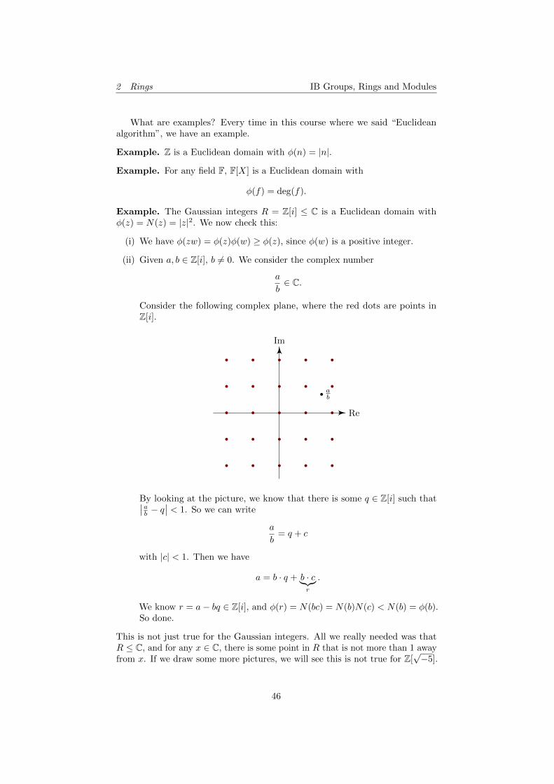
2 Rings IB Groups, Rings and Modules
What are examples? Every time in this course where we said “Euclideanalgorithm”, we have an example.
Example. Z is a Euclidean domain with φ(n) = |n|.
Example. For any field F, F[X] is a Euclidean domain with
φ(f) = deg(f).
Example. The Gaussian integers R = Z[i] ≤ C is a Euclidean domain withφ(z) = N(z) = |z|2. We now check this:
(i) We have φ(zw) = φ(z)φ(w) ≥ φ(z), since φ(w) is a positive integer.
(ii) Given a, b ∈ Z[i], b 6= 0. We consider the complex number
a
b∈ C.
Consider the following complex plane, where the red dots are points inZ[i].
Re
Im
ab
By looking at the picture, we know that there is some q ∈ Z[i] such that∣∣ab − q
∣∣ < 1. So we can write
a
b= q + c
with |c| < 1. Then we have
a = b · q + b · c︸︷︷︸r
.
We know r = a− bq ∈ Z[i], and φ(r) = N(bc) = N(b)N(c) < N(b) = φ(b).So done.
This is not just true for the Gaussian integers. All we really needed was thatR ≤ C, and for any x ∈ C, there is some point in R that is not more than 1 awayfrom x. If we draw some more pictures, we will see this is not true for Z[
√−5].
46
2 Rings IB Groups, Rings and Modules
Before we move on to prove unique factorization, we first derive somethingwe’ve previously mentioned. Recall we showed that every ideal in Z is principal,and we proved this by the Euclidean algorithm. So we might expect this to betrue in an arbitrary Euclidean domain.
Definition (Principal ideal domain). A ring R is a principal ideal domain (PID)if it is an integral domain, and every ideal is a principal ideal, i.e. for all I CR,there is some a such that I = (a).
Example. Z is a principal ideal domain.
Proposition. Let R be a Euclidean domain. Then R is a principal ideal domain.
We have already proved this, just that we did it for a particular Euclideandomain Z. Nonetheless, we shall do it again.
Proof. Let R have a Euclidean function φ : R \ 0 → Z≥0. We let I CR be anon-zero ideal, and let b ∈ I \ 0 be an element with φ(b) minimal. Then forany a ∈ I, we write
a = bq + r,
with r = 0 or φ(r) < φ(b). However, any such r must be in I since r = a−bq ∈ I.So we cannot have φ(r) < φ(b). So we must have r = 0. So a = bq. So a ∈ (b).Since this is true for all a ∈ I, we must have I ⊆ (b). On the other hand, sinceb ∈ I, we must have (b) ⊆ I. So we must have I = (b).
This is exactly, word by word, the same proof as we gave for the integers,except we replaced the absolute value with φ.
Example. Z is a Euclidean domain, and hence a principal ideal domain. Also,for any field F, F[X] is a Euclidean domain, hence a principal ideal domain.
Also, Z[i] is a Euclidean domain, and hence a principal ideal domain.What is a non-example of principal ideal domains? In Z[X], the ideal
(2, X)CZ[X] is not a principal ideal. Suppose it were. Then (2, X) = (f). Since2 ∈ (2, X) = (f), we know 2 ∈ (f) , i.e. 2 = f · g for some g. So f has degreezero, and hence constant. So f = ±1 or ±2.
If f = ±1, since ±1 are units, then (f) = Z[X]. But (2, X) 6= Z[X], since,say, 1 6∈ (2, X). If f = ±2, then since X ∈ (2, X) = (f), we must have ±2 | X,but this is clearly false. So (2, X) cannot be a principal ideal.
Example. Let A ∈ Mn×n(F) be an n × n matrix over a field F. We considerthe following set
I = f ∈ F[X] : f(A) = 0.
This is an ideal — if f, g ∈ I, then (f + g)(A) = f(A) + g(A) = 0. Similarly, iff ∈ I and h ∈ F[X], then (fg)(A) = f(A)g(A) = 0.
But we know F[X] is a principal ideal domain. So there must be somem ∈ F[X] such that I = (m) for some m.
Suppose f ∈ F[X] such that f(A) = 0, i.e. f ∈ I. Then m | f . So m isa polynomial that divides all polynomials that kill A, i.e. m is the minimalpolynomial of A.
We have just proved that all matrices have minimal polynomials, and thatthe minimal polynomial divides all other polynomials that kill A. Also, theminimal polynomial is unique up to multiplication of units.
47
2 Rings IB Groups, Rings and Modules
Let’s get further into number theory-like things. For a general ring, wecannot factorize things into irreducibles uniquely. However, in some rings, thisis possible.
Definition (Unique factorization domain). An integral domain R is a uniquefactorization domain (UFD) if
(i) Every non-unit may be written as a product of irreducibles;
(ii) If p1p2 · · · pn = q1 · · · qm with pi, qj irreducibles, then n = m, and they canbe reordered such that pi is an associate of qi.
This is a really nice property, and here we can do things we are familiar within number theory. So how do we know if something is a unique factorizationdomain?
Our goal is to show that all principal ideal domains are unique factorizationdomains. To do so, we are going to prove several lemmas that give us somereally nice properties of principal ideal domains.
Recall we saw that every prime is an irreducible, but in Z[√−5], there are
some irreducibles that are not prime. However, this cannot happen in principalideal domains.
Lemma. Let R be a principal ideal domain. If p ∈ R is irreducible, then it isprime.
Note that this is also true for general unique factorization domains, whichwe can prove directly by unique factorization.
Proof. Let p ∈ R be irreducible, and suppose p | a · b. Also, suppose p - a. Weneed to show p | b.
Consider the ideal (p, a)CR. Since R is a principal ideal domain, there issome d ∈ R such that (p, a) = (d). So d | p and d | a.
Since d | p, there is some q1 such that p = q1d. As p is irreducible, either q1
or d is a unit.If q1 is a unit, then d = q−1
1 p, and this divides a. So a = q−11 px for some x.
This is a contradiction, since p - a.Therefore d is a unit. So (p, a) = (d) = R. In particular, 1R ∈ (p, a). So
suppose 1R = rp + sa, for some r, s ∈ R. We now take the whole thing andmultiply by b. Then we get
b = rpb+ sab.
We observe that ab is divisible by p, and so is p. So b is divisible by p. Sodone.
This is similar to the argument for integers. For integers, we would say if p - a,then p and a are coprime. Therefore there are some r, s such that 1 = rp+ sa.Then we continue the proof as above. Hence what we did in the middle is to dosomething similar to showing p and a are “coprime”.
Another nice property of principal ideal domains is the following:
Lemma. Let R be a principal ideal domain. Let I1 ⊆ I2 ⊆ I3 ⊆ · · · be a chainof ideals. Then there is some N ∈ N such that In = In+1 for some n ≥ N .
48
2 Rings IB Groups, Rings and Modules
So in a principal ideal domain, we cannot have an infinite chain of biggerand bigger ideals.
Definition (Ascending chain condition). A ring satisfies the ascending chaincondition (ACC) if there is no infinite strictly increasing chain of ideals.
Definition (Noetherian ring). A ring that satisfies the ascending chain conditionis known as a Noetherian ring.
So we are proving that every principal ideal domain is Noetherian.
Proof. The obvious thing to do when we have an infinite chain of ideals is totake the union of them. We let
I =
∞⋃n≥1
In,
which is again an ideal. Since R is a principal ideal domain, I = (a) for somea ∈ R. We know a ∈ I =
⋃∞n=0 In. So a ∈ IN for some N . Then we have
(a) ⊆ IN ⊆ I = (a)
So we must have IN = I. So In = IN = I for all n ≥ N .
Notice it is not important that I is generated by one element. If, for somereason, we know I is generated by finitely many elements, then the same argumentwork. So if every ideal is finitely generated, then the ring must be Noetherian.It turns out this is an if-and-only-if — if you are Noetherian, then every ideal isfinitely generated. We will prove this later on in the course.
Finally, we have done the setup, and we can prove the proposition promised.
Proposition. Let R be a principal ideal domain. Then R is a unique factoriza-tion domain.
Proof. We first need to show any (non-unit) r ∈ R is a product of irreducibles.Suppose r ∈ R cannot be factored as a product of irreducibles. Then it is
certainly not irreducible. So we can write r = r1s1, with r1, s1 both non-units.Since r cannot be factored as a product of irreducibles, wlog r1 cannot befactored as a product of irreducibles (if both can, then r would be a product ofirreducibles). So we can write r1 = r2s2, with r2, s2 not units. Again, wlog r2
cannot be factored as a product of irreducibles. We continue this way.By assumption, the process does not end, and then we have the following
chain of ideals:(r) ⊆ (r1) ⊆ (r2) ⊆ · · · ⊆ (rn) ⊆ · · ·
But then we have an ascending chain of ideals. By the ascending chain condition,these are all eventually equal, i.e. there is some n such that (rn) = (rn+1) =(rn+2) = · · · . In particular, since (rn) = (rn+1), and rn = rn+1sn+1, then sn+1
is a unit. But this is a contradiction, since sn+1 is not a unit. So r must be aproduct of irreducibles.
To show uniqueness, we let p1p2 · · · pn = q1q2 · · · qm, with pi, qi irreducible.So in particular p1 | q1 · · · qm. Since p1 is irreducible, it is prime. So p1 dividessome qi. We reorder and suppose p1 | q1. So q1 = p1 · a for some a. But since q1
49
2 Rings IB Groups, Rings and Modules
is irreducible, a must be a unit. So p1, q1 are associates. Since R is a principalideal domain, hence integral domain, we can cancel p1 to obtain
p2p3 · · · pn = (aq2)q3 · · · qm.
We now rename aq2 as q2, so that we in fact have
p2p3 · · · pn = q2q3 · · · qm.
We can then continue to show that pi and qi are associates for all i. This alsoshows that n = m, or else if n = m + k, saw, then pk+1 · · · pn = 1, which is acontradiction.
We can now use this to define other familiar notions from number theory.
Definition (Greatest common divisor). d is a greatest common divisor (gcd) ofa1, a2, · · · , an if d | ai for all i, and if any other d′ satisfies d′ | ai for all i, thend′ | d.
Note that the gcd of a set of numbers, if exists, is not unique. It is onlywell-defined up to a unit.
This is a definition that says what it means to be a greatest common divisor.However, it does not always have to exist.
Lemma. Let R be a unique factorization domain. Then greatest commondivisors exists, and is unique up to associates.
Proof. We construct the greatest common divisor using the good-old way ofprime factorization.
We let p1, p2, · · · , pm be a list of all irreducible factors of ai, such that notwo of these are associates of each other. We now write
ai = ui
m∏j=1
pnijj ,
where nij ∈ N and ui are units. We let
mj = mininij,
and choose
d =
m∏j=1
pmjj .
As, by definition, mj ≤ nij for all i, we know d | ai for all i.Finally, if d′ | ai for all i, then we let
d′ = v
m∏j=1
ptjj .
Then we must have tj ≤ nij for all i, j. So we must have tj ≤ mj for all j. Sod′ | d.
Uniqueness is immediate since any two greatest common divisors have todivide each other.
50
2 Rings IB Groups, Rings and Modules
2.5 Factorization in polynomial rings
Since polynomial rings are a bit more special than general integral domains, wecan say a bit more about them.
Recall that for F a field, we know F [X] is a Euclidean domain, hence aprincipal ideal domain, hence a unique factorization domain. Therefore we know
(i) If I C F [X], then I = (f) for some f ∈ F [X].
(ii) If f ∈ F [X], then f is irreducible if and only if f is prime.
(iii) Let f be irreducible, and suppose (f) ⊆ J ⊆ F [X]. Then J = (g) for someg. Since (f) ⊆ (g), we must have f = gh for some h. But f is irreducible.So either g or h is a unit. If g is a unit, then (g) = F [X]. If h is a unit,then (f) = (g). So (f) is a maximal ideal. Note that this argument is validfor any PID, not just polynomial rings.
(iv) Let (f) be a prime ideal. Then f is prime. So f is irreducible. So (f) ismaximal. But we also know in complete generality that maximal ideals areprime. So in F [X], prime ideals are the same as maximal ideals. Again,this is true for all PIDs in general.
(v) Thus f is irreducible if and only if F [X]/(f) is a field.
To use the last item, we can first show that F [X]/(f) is a field, and then use thisto deduce that f is irreducible. But we can also do something more interesting
— find an irreducible f , and then generate an interesting field F [X]/(f).So we want to understand reducibility, i.e. we want to know whether we can
factorize a polynomial f . Firstly, we want to get rid of the trivial case where wejust factor out a scalar, e.g. 2X2 +2 = 2(X2 +1) ∈ Z[X] is a boring factorization.
Definition (Content). Let R be a UFD and f = a0 +a1X+ · · ·+anXn ∈ R[X].
The content c(f) of f is
c(f) = gcd(a0, a1, · · · , an) ∈ R.
Again, since the gcd is only defined up to a unit, so is the content.
Definition (Primitive polynomial). A polynomial is primitive if c(f) is a unit,i.e. the ai are coprime.
Note that this is the best we can do. We cannot ask for c(f) to be exactly 1,since the gcd is only well-defined up to a unit.
We now want to prove the following important lemma:
Lemma (Gauss’ lemma). Let R be a UFD, and f ∈ R[X] be a primitivepolynomial. Then f is reducible in R[X] if and only if f is reducible F [X], whereF is the field of fractions of R.
We can’t do this right away. We first need some preparation. Before that,we do some examples.
Example. Consider X3 +X + 1 ∈ Z[X]. This has content 1 so is primitive. Weshow it is not reducible in Z[X], and hence not reducible in Q[X].
51
2 Rings IB Groups, Rings and Modules
Suppose f is reducible in Q[X]. Then by Gauss’ lemma, this is reducible inZ[X]. So we can write
X3 +X + 1 = gh,
for some polynomials g, h ∈ Z[X], with g, h not units. But if g and h are notunits, then they cannot be constant, since the coefficients of X3 +X + 1 are all1 or 0. So they have degree at least 1. Since the degrees add up to 3, we wlogsuppose g has degree 1 and h has degree 2. So suppose
g = b0 + b1X, h = c0 + c1X + c2X2.
Multiplying out and equating coefficients, we get
b0c0 = 1
c2b1 = 1
So b0 and b1 must be ±1. So g is either 1 +X, 1−X,−1 +X or −1−X, andhence has ±1 as a root. But this is a contradiction, since ±1 is not a root ofX3 +X + 1. So f is not reducible in Q. In particular, f has no root in Q.
We see the advantage of using Gauss’ lemma — if we worked in Q instead,we could have gotten to the step b0c0 = 1, and then we can do nothing, since b0and c0 can be many things if we live in Q.
Now we start working towards proving this.
Lemma. Let R be a UFD. If f, g ∈ R[X] are primitive, then so is fg.
Proof. We let
f = a0 + a1X + · · ·+ anXn,
g = b0 + b1X + · · ·+ bmXm,
where an, bm 6= 0, and f, g are primitive. We want to show that the content offg is a unit.
Now suppose fg is not primitive. Then c(fg) is not a unit. Since R is aUFD, we can find an irreducible p which divides c(fg).
By assumption, c(f) and c(g) are units. So p - c(f) and p - c(g). So supposep | a0, p | a1, . . . , p | ak−1 but p - ak. Note it is possible that k = 0. Similarly,suppose p | b0, p | b1, · · · , p | b`−1, p - b`.
We look at the coefficient of Xk+` in fg. It is given by∑i+j=k+`
aibj = ak+`b0 + · · ·+ ak+1b`−1 + akb` + ak−1b`+1 + · · ·+ a0b`+k.
By assumption, this is divisible by p. So
p |∑
i+j=k+`
aibj .
However, the terms ak+`b0 + · · ·+ ak+1b`−1, is divisible by p, as p | bj for j < `.Similarly, ak−1b`+1 + · · · + a0b`+k is divisible by p. So we must have p | akb`.As p is irreducible, and hence prime, we must have p | ak or p | b`. This is acontradiction. So c(fg) must be a unit.
52
2 Rings IB Groups, Rings and Modules
Corollary. Let R be a UFD. Then for f, g ∈ R[X], we have that c(fg) is anassociate of c(f)c(g).
Again, we cannot say they are equal, since content is only well-defined up toa unit.
Proof. We can write f = c(f)f1 and g = c(g)g1, with f1 and g1 irreducible.Then
fg = c(f)c(g)f1g1.
Since f1g1 is primitive, so c(f)c(g) is a gcd of the coefficients of fg, and so isc(fg), by definition. So they are associates.
Finally, we can prove Gauss’ lemma.
Lemma (Gauss’ lemma). Let R be a UFD, and f ∈ R[X] be a primitivepolynomial. Then f is reducible in R[X] if and only if f is reducible F [X], whereF is the field of fractions of R.
Proof. We will show that a primitive f ∈ R[X] is reducible in R[X] if and onlyif f is reducible in F [X].
One direction is almost immediately obvious. Let f = gh be a product inR[X] with g, h not units. As f is primitive, so are g and h. So both have degree> 0. So g, h are not units in F [X]. So f is reducible in F [X].
The other direction is less obvious. We let f = gh in F [X], with g, h not units.So g and h have degree > 0, since F is a field. So we can clear denominatorsby finding a, b ∈ R such that (ag), (bh) ∈ R[X] (e.g. let a be the product ofdenominators of coefficients of g). Then we get
abf = (ag)(bh),
and this is a factorization in R[X]. Here we have to be careful — (ag) is onething that lives in R[X], and is not necessarily a product in R[X], since g mightnot be in R[X]. So we should just treat it as a single symbol.
We now write
(ag) = c(ag)g1,
(bh) = c(bh)h1,
where g1, h1 are primitive. So we have
ab = c(abf) = c((ag)(bh)) = u · c(ag)c(bh),
where u ∈ R is a unit, by the previous corollary. But also we have
abf = c(ag)c(gh)g1h1 = u−1abg1h1.
So cancelling ab givesf = u−1g1h1 ∈ R[X].
So f is reducible in R[X].
If this looks fancy and magical, you can try to do this explicitly in the casewhere R = Z and F = Q. Then you will probably get enlightened.
We will do another proof performed in a similar manner.
53
2 Rings IB Groups, Rings and Modules
Proposition. Let R be a UFD, and F be its field of fractions. Let g ∈ R[X]be primitive. We let
J = (g)CR[X], I = (g)C F [X].
ThenJ = I ∩R[X].
In other words, if f ∈ R[X] and we can write it as f = gh, with h ∈ F [X], thenin fact h ∈ R[X].
Proof. The strategy is the same — we clear denominators in the equation f = gh,and then use contents to get that down in R[X].
We certainly have J ⊆ I ∩R[X]. Now let f ∈ I ∩R[X]. So we can write
f = gh,
with h ∈ F [X]. So we can choose b ∈ R such that bh ∈ R[X]. Then we know
bf = g(bh) ∈ R[X].
We let(bh) = c(bh)h1,
for h1 ∈ R[X] primitive. Thus
bf = c(bh)gh1.
Since g is primitive, so is gh1. So c(bh) = uc(bf) for u a unit. But bf is really aproduct in R[X]. So we have
c(bf) = c(b)c(f) = bc(f).
So we havebf = ubc(f)gh1.
Cancelling b givesf = g(uc(f)h1).
So g | f in R[X]. So f ∈ J .
From this we can get ourselves a large class of UFDs.
Theorem. If R is a UFD, then R[X] is a UFD.
In particular, if R is a UFD, then R[X1, · · · , Xn] is also a UFD.
Proof. We know R[X] has a notion of degree. So we will combine this with thefact that R is a UFD.
Let f ∈ R[X]. We can write f = c(f)f1, with f1 primitive. Firstly, as R is aUFD, we may factor
c(f) = p1p2 · · · pn,
for pi ∈ R irreducible (and also irreducible in R[X]). Now we want to deal withf1.
54
2 Rings IB Groups, Rings and Modules
If f1 is not irreducible, then we can write
f1 = f2f3,
with f2, f3 both not units. Since f1 is primitive, f2, f3 also cannot be constants.So we must have deg f2,deg f3 > 0. Also, since deg f2 +deg f3 = deg f1, we musthave deg f2,deg f3 < deg f1. If f2, f3 are irreducible, then done. Otherwise, keepon going. We will eventually stop since the degrees have to keep on decreasing.So we can write it as
f1 = q1 · · · qm,
with qi irreducible. So we can write
f = p1p2 · · · pnq1q2 · · · qm,
a product of irreducibles.For uniqueness, we first deal with the p’s. We note that
c(f) = p1p2 · · · pn
is a unique factorization of the content, up to reordering and associates, as R isa UFD. So cancelling the content, we only have to show that primitives can befactored uniquely.
Suppose we have two factorizations
f1 = q1q2 · · · qm = r1r2 · · · r`.
Note that each qi and each ri is a factor of the primitive polynomial f1, so arealso primitive. Now we do (maybe) the unexpected thing. We let F be the fieldof fractions of R, and consider qi, ri ∈ F [X]. Since F is a field, F is a Euclideandomain, hence principal ideal domain, hence unique factorization domain.
By Gauss’ lemma, since the qi and ri are irreducible in R[X], they are alsoirreducible in F [X]. As F [X] is a UFD, we find that ` = m, and after reordering,ri and qi are associates, say
ri = uiqi,
with ui ∈ F [X] a unit. What we want to say is that ri is a unit times qi in R[X].Firstly, note that ui ∈ F as it is a unit. Clearing denominators, we can write
airi = biqi ∈ R[X].
Taking contents, since ri, qi are primitives, we know ai and bi are associates, say
bi = viai,
with vi ∈ R a unit. Cancelling ai on both sides, we know ri = viqi as required.
The key idea is to use Gauss’ lemma to say the reducibility in R[X] is thesame as reducibility in F [X], as long as we are primitive. The first part aboutcontents is just to turn everything into primitives.
Note that the last part of the proof is just our previous proposition. Wecould have applied it, but we decide to spell it out in full for clarity.
Example. We know Z[X] is a UFD, and if R is a UFD, then R[X1, · · · , Xn] isalso a UFD.
55
2 Rings IB Groups, Rings and Modules
This is a useful thing to know. In particular, it gives us examples of UFDsthat are not PIDs. However, in such rings, we would also like to have an easy todetermine whether something is reducible. Fortunately, we have the followingcriterion:
Proposition (Eisenstein’s criterion). Let R be a UFD, and let
f = a0 + a1X + · · ·+ anXn ∈ R[X]
be primitive with an 6= 0. Let p ∈ R be irreducible (hence prime) be such that
(i) p - an;
(ii) p | ai for all 0 ≤ i < n;
(iii) p2 - a0.
Then f is irreducible in R[X], and hence in F [X] (where F is the field of fractionsof F ).
It is important that we work in R[X] all the time, until the end where weapply Gauss’ lemma. Otherwise, we cannot possibly apply Eisenstein’s criterionsince there are no primes in F .
Proof. Suppose we have a factorization f = gh with
g = r0 + r1X + · · ·+ rkXk
h = s0 + s1X + · · ·+ s`X`,
for rk, s` 6= 0.We know rks` = an. Since p - an, so p - rk and p - s`. We can also look
at bottom coefficients. We know r0s0 = a0. We know p | a0 and p2 - a0. So pdivides exactly one of r0 and s0. wlog, p | r0 and p - s0.
Now let j be such that
p | r0, p | r1, · · · , p | rj−1, p - rj .
We now look at aj . This is, by definition,
aj = r0sj + r1sj−1 + · · ·+ rj−1s1 + rjs0.
We know r0, · · · , rj−1 are all divisible by p. So
p | r0sj + r1sj−1 + · · ·+ rj−1s1.
Also, since p - rj and p - s0, we know p - rjs0, using the fact that p is prime. Sop - aj . So we must have j = n.
We also know that j ≤ k ≤ n. So we must have j = k = n. So deg g = n.Hence ` = n− h = 0. So h is a constant. But we also know f is primitive. So hmust be a unit. So this is not a proper factorization.
Example. Consider the polynomial Xn − p ∈ Z[X] for p a prime. ApplyEisenstein’s criterion with p, and observe all the conditions hold. This iscertainly primitive, since this is monic. So Xn − p is irreducible in Z[X], hencein Q[X]. In particular, Xn − p has no rational roots, i.e. n
√p is irrational (for
n > 1).
56
2 Rings IB Groups, Rings and Modules
Example. Consider a polynomial
f = Xp−1 +Xp−2 + · · ·+X2 +X + 1 ∈ Z[X],
where p is a prime number. If we look at this, we notice Eisenstein’s criteriadoes not apply. What should we do? We observe that
f =Xp − 1
X − 1.
So it might be a good idea to let Y = X − 1. Then we get a new polynomial
f = f(Y ) =(Y + 1)p − 1
Y= Y p−1 +
(p
1
)Y p−2 +
(p
2
)Y p−3 + · · ·+
(p
p− 1
).
When we look at it hard enough, we notice Eisenstein’s criteria can be applied —we know p |
(pi
)for 1 ≤ i ≤ p− 1, but p2 -
(pp−1
)= p. So f is irreducible in Z[Y ].
Now if we had a factorization
f(X) = g(X)h(X) ∈ Z[X],
then we getf(Y ) = g(Y + 1)h(Y + 1)
in Z[Y ]. So f is irreducible.Hence none of the roots of f are rational (but we already know that — they
are not even real!).
2.6 Gaussian integers
We’ve mentioned the Gaussian integers already.
Definition (Gaussian integers). The Gaussian integers is the subring
Z[i] = a+ bi : a, b ∈ Z ≤ C.
We have already shown that the norm N(a + ib) = a2 + b2 is a Euclideanfunction for Z[i]. So Z[i] is a Euclidean domain, hence principal ideal domain,hence a unique factorization domain.
Since the units must have norm 1, they are precisely ±1,±i. What doesfactorization in Z[i] look like? What are the primes? We know we are going toget new primes, i.e. primes that are not integers, while we will lose some otherprimes. For example, we have
2 = (1 + i)(1− i).
So 2 is not irreducible, hence not prime. However, 3 is a prime. We haveN(3) = 9. So if 3 = uv, with u, v not units, then 9 = N(u)N(v), and neitherN(u) nor N(v) are 1. So N(u) = N(v) = 3. However, 3 = a2 + b2 has nosolutions with a, b ∈ Z. So there is nothing of norm 3. So 3 is irreducible, hencea prime.
Also, 5 is not prime, since
5 = (1 + 2i)(1− 2i).
How can we understand which primes stay as primes in the Gaussian integers?
57
2 Rings IB Groups, Rings and Modules
Proposition. A prime number p ∈ Z is prime in Z[i] if and only if p 6= a2 + b2
for a, b ∈ Z \ 0.
The proof is exactly what we have done so far.
Proof. If p = a2 + b2, then p = (a+ ib)(a− ib). So p is not irreducible.Now suppose p = uv, with u, v not units. Taking norms, we get p2 =
N(u)N(v). So if u and v are not units, then N(u) = N(v) = p. Writingu = a+ ib, then this says a2 + b2 = p.
So what we have to do is to understand when a prime p can be written as asum of two squares. We will need the following helpful lemma:
Lemma. Let p be a prime number. Let Fp = Z/pZ be the field with p elements.Let F×p = Fp \0 be the group of invertible elements under multiplication. ThenF×p ∼= Cp−1.
Proof. Certainly F×p has order p− 1, and is abelian. We know from the classifi-cation of finite abelian groups that if F×p is not cyclic, then it must contain asubgroup Cm ×Cm for m > 1 (we can write it as Cd ×Cd′ × · · · , and that d′ | d.So Cd has a subgroup isomorphic to Cd′).
We consider the polynomial Xm − 1 ∈ Fp[x], which is a UFD. At best, thisfactors into m linear factors. So Xm − 1 has at most m distinct roots. But ifCm × Cm ≤ F×p , then we can find m2 elements of order diving m. So there arem2 elements of Fp which are roots of Xm − 1. This is a contradiction. So F×p iscyclic.
This is a funny proof, since we have not found any element that has orderp− 1.
Proposition. The primes in Z[i] are, up to associates,
(i) Prime numbers p ∈ Z ≤ Z[i] such that p ≡ 3 (mod 4).
(ii) Gaussian integers z ∈ Z[i] with N(z) = zz = p for some prime p such thatp = 2 or p ≡ 1 (mod 4).
Proof. We first show these are primes. If p ≡ 3 (mod 4), then p 6= a2 + b2, sincea square number mod 4 is always 0 or 1. So these are primes in Z[i].
On the other hand, if N(z) = p, and z = uv, then N(u)N(v) = p. So N(u)is 1 or N(v) is 1. So u or v is a unit. Note that we did not use the conditionthat p 6≡ 3 (mod 4). This is not needed, since N(z) is always a sum of squares,and hence N(z) cannot be a prime that is 3 mod 4.
Now let z ∈ Z[i] be irreducible, hence prime. Then z is also irreducible. SoN(z) = zz is a factorization of N(z) into irreducibles. Let p ∈ Z be an ordinaryprime number dividing N(z), which exists since N(z) 6= 1.
Now if p ≡ 3 (mod 4), then p itself is prime in Z[i] by the first part of theproof. So p | N(z) = zz. So p | z or p | z. Note that if p | z, then p | z by takingcomplex conjugates. So we get p | z. Since both p and z are both irreducible,they must be equal up to associates.
Otherwise, we get p = 2 or p ≡ 1 (mod 4). If p ≡ 1 (mod 4), then p−1 = 4kfor some k ∈ Z. As F×p ∼= Cp−1 = C4k, there is a unique element of order 2 (thisis true for any cyclic group of order 4k — think Z/4kZ). This must be [−1] ∈ Fp.Now let a ∈ F×p be an element of order 4. Then a2 has order 2. So [a2] = [−1].
58
2 Rings IB Groups, Rings and Modules
This is a complicated way of saying we can find an a such that p | a2 + 1.Thus p | (a+ i)(a− i). In the case where p = 2, we know by checking directlythat 2 = (1 + i)(1− i).
In either case, we deduce that p (or 2) is not prime (hence irreducible),since it clearly does not divide a ± i (or 1 ± i). So we can write p = z1z2, forz1, z2 ∈ Z[i] not units. Now we get
p2 = N(p) = N(z1)N(z2).
As the zi are not units, we know N(z1) = N(z2) = p. By definition, this meansp = z1z1 = z2z2. But also p = z1z2. So we must have z1 = z2.
Finally, we have p = z1z1 | N(z) = zz. All these z, zi are irreducible. So zmust be an associate of z1 (or maybe z1). So in particular N(z) = p.
Corollary. An integer n ∈ Z≥0 may be written as x2 + y2 (as the sum of twosquares) if and only if “when we write n = pn1
1 pn22 · · · p
nkk as a product as distinct
primes, then pi ≡ 3 (mod 4) implies ni is even”.
We have proved this in the case when n is a prime.
Proof. If n = x2 + y2, then we have
n = (x+ iy)(x− iy) = N(x+ iy).
Let z = x+ iy. So we can write z = α1 · · ·αq as a product of irreducibles in Z[i].By the proposition, each αi is either αi = p (a genuine prime number with p ≡ 3(mod 4)), or N(αi) = p is a prime number which is either 2 or ≡ 1 (mod 4). Wenow take the norm to obtain
N = x2 + y2 = N(z) = N(α1)N(α2) · · ·N(αq).
Now each N(αi) is either p2 with p ≡ 3 (mod 4), or is just p for p = 2 or p ≡ 1(mod 4). So if pm is the largest power of p divides n, we find that n must beeven if p ≡ 3 (mod 4).
Conversely, let n = pn11 pn2
2 · · · pnkk be a product of distinct primes. Now for
each pi, either pi ≡ 3 (mod 4), and ni is even, in which case
pnii = (p2i )ni/2 = N(p
ni/2i );
or pi = 2 or pi ≡ 1 (mod 4), in which case, the above proof shows that pi = N(αi)for some αi. So pni = N(αni ).
Since the norm is multiplicative, we can write n as the norm of some z ∈ Z[i].So
n = N(z) = N(x+ iy) = x2 + y2,
as required.
Example. We know 65 = 5×13. Since 5, 13 ≡ 1 (mod 4), it is a sum of squares.Moreover, the proof tells us how to find 65 as the sum of squares. We have tofactor 5 and 13 in Z[i]. We have
5 = (2 + i)(2− i)13 = (2 + 3i)(2− 3i).
59
2 Rings IB Groups, Rings and Modules
So we know
65 = N(2 + i)N(2 + 3i) = N((2 + i)(2 + 3i)) = N(1 + 8i) = 12 + 82.
But there is a choice here. We had to pick which factor is α and which is α. Sowe can also write
65 = N((2 + i)(2− 3i)) = N(7− 4i) = 72 + 42.
So not only are we able to write them as sum of squares, but this also gives usmany ways of writing 65 as a sum of squares.
2.7 Algebraic integers
We generalize the idea of Gaussian integers to algebraic integers.
Definition (Algebraic integer). An α ∈ C is called an algebraic integer if it isa root of a monic polynomial in Z[X], i.e. there is a monic f ∈ Z[X] such thatf(α) = 0.
We can immediately check that this is a sensible definition — not all complexnumbers are algebraic integers, since there are only countably many polynomialswith integer coefficients, hence only countably many algebraic integers, but thereare uncountably many complex numbers.
Notation. For α an algebraic integer, we write Z[α] ∈ C for the smallest subringcontaining α.
This can also be defined for arbitrary complex numbers, but it is less inter-esting.
We can also construct Z[α] by taking it as the image of the map φ : Z[X]→ Cgiven by g 7→ g(α). So we can also write
Z[α] =Z[X]
I, I = kerφ.
Note that I is non-empty, since, say, f ∈ I, by definition of an algebraic integer.
Proposition. Let α ∈ C be an algebraic integer. Then the ideal
I = ker(φ : Z[X]→ C, f 7→ f(α))
is principal, and equal to (fα) for some irreducible monic fα.
This is a non-trivial theorem, since Z[X] is not a principal ideal domain. Sothere is no immediate guarantee that I is generated by one polynomial.
Definition (Minimal polynomial). Let α ∈ C be an algebraic integer. Thenthe minimal polynomial is a polynomial fα is the irreducible monic such thatI = ker(φ) = (fα).
Proof. By definition, there is a monic f ∈ Z[X] such that f(a) = 0. So f ∈ I.So I 6= 0. Now let fα ∈ I be such a polynomial of minimal degree. We maysuppose that fα is primitive. We want to show that I = (fα), and that fα isirreducible.
60
2 Rings IB Groups, Rings and Modules
Let h ∈ I. We pretend we are living in Q[X]. Then we have the Euclideanalgorithm. So we can write
h = fαq + r,
with r = 0 or deg r < deg fα. This was done over Q[X], not Z[X]. We now cleardenominators. We multiply by some a ∈ Z to get
ah = fα(aq) + (ar),
where now (aq), (ar) ∈ Z[X]. We now evaluate these polynomials at α. Thenwe have
ah(α) = fα(α)aq(α) + ar(α).
We know fα(α) = h(α) = 0, since fα and h are both in I. So ar(α) = 0. So(ar) ∈ I. As fα ∈ I has minimal degree, we cannot have deg(r) = deg(ar) <deg(fa). So we must have r = 0.
Hence we knowah = fα · (aq)
is a factorization in Z[X]. This is almost right, but we want to factor h, not ah.Again, taking contents of everything, we get
ac(h) = c(ah) = c(fα(aq)) = c(aq),
as fα is primitive. In particular, a | c(aq). This, by definition of content, means(aq) can be written as aq, where q ∈ Z[X]. Cancelling, we get q = q ∈ Z[X]. Sowe know
h = fαq ∈ (fα).
So we know I = (fα).To show fα is irreducible, note that
Z[X]
(fα)∼=
Z[X]
kerφ∼= im(φ) = Z[α] ≤ C.
Since C is an integral domain, so is im(φ). So we know Z[X]/(fα) is an integraldomain. So (fα) is prime. So fα is prime, hence irreducible.
If this final line looks magical, we can unravel this proof as follows: supposefα = pq for some non-units pq. Then since fα(α) = 0, we know p(α)q(α) = 0.Since p(α), q(α) ∈ C, which is an integral domain, we must have, say, p(α) = 0.But then deg p < deg fα, so p 6∈ I = (fα). Contradiction.
Example.
(i) We know α = i is an algebraic integer with fα = X2 + 1.
(ii) Also, α =√
2 is an algebraic integer with fα = X2 − 2.
(iii) More interestingly, α = 12 (1 +
√−3) is an algebraic integer with fα =
X2 −X − 1.
(iv) The polynomial X5 −X + d ∈ Z[X] with d ∈ Z≥0 has precisely one realroot α, which is an algebraic integer. It is a theorem, which will be provedin IID Galois Theory, that this α cannot be constructed from integersvia +,−,×,÷, n
√· . It is also a theorem, found in IID Galois Theory, that
degree 5 polynomials are the smallest degree for which this can happen (theprove involves writing down formulas analogous to the quadratic formulafor degree 3 and 4 polynomials).
61
2 Rings IB Groups, Rings and Modules
Lemma. Let α ∈ Q be an algebraic integer. Then α ∈ Z.
Proof. Let fα ∈ Z[X] be the minimal polynomial, which is irreducible. In Q[X],the polynomial X − α must divide fα. However, by Gauss’ lemma, we knowf ∈ Q[X] is irreducible. So we must have fα = X − α ∈ Z[X]. So α is aninteger.
It turns out the collection of all algebraic integers form a subring of C. Thisis not at all obvious — given f, g ∈ Z[X] monic such that f(α) = g(α) = 0, thereis no easy way to find a new monic h such that h(α+ β) = 0. We will prove thismuch later on in the course.
2.8 Noetherian rings
We now revisit the idea of Noetherian rings, something we have briefly mentionedwhen proving that PIDs are UFDs.
Definition (Noetherian ring). A ring is Noetherian if for any chain of ideals
I1 ⊆ I2 ⊆ I3 ⊆ · · · ,
there is some N such that IN = IN+1 = IN+2 = · · · .This condition is known as the ascending chain condition.
Example. Every finite ring is Noetherian. This is since there are only finitelymany possible ideals.
Example. Every field is Noetherian. This is since there are only two possibleideals.
Example. Every principal ideal domain (e.g. Z) is Noetherian. This is easy tocheck directly, but the next proposition will make this utterly trivial.
Most rings we love and know are indeed Noetherian. However, we canexplicitly construct some non-Noetherian ideals.
Example. The ring Z[X1, X2, X3, · · · ] is not Noetherian. This has the chain ofstrictly increasing ideals
(X1) ⊆ (X1, X2) ⊆ (X1, X2, X3) ⊆ · · · .
We have the following proposition that makes Noetherian rings much moreconcrete, and makes it obvious why PIDs are Noetherian.
Definition (Finitely generated ideal). An ideal I is finitely generated if it canbe written as I = (r1, · · · , rn) for some r1, · · · , rn ∈ R.
Proposition. A ring is Noetherian if and only if every ideal is finitely generated.
Every PID trivially satisfies this condition. So we know every PID is Noethe-rian.
62
2 Rings IB Groups, Rings and Modules
Proof. We start with the easier direction — from concrete to abstract.Suppose every ideal of R is finitely generated. Given the chain I1 ⊆ I2 ⊆ · · · ,
consider the idealI = I1 ∪ I2 ∪ I3 ∪ · · · .
This is obviously an ideal, and you will check this manually in example sheet 2.We know I is finitely generated, say I = (r1, · · · , rn), with ri ∈ Iki . Let
K = maxi=1,··· ,n
ki.
Then r1, · · · , rn ∈ IK . So IK = I. So IK = IK+1 = IK+2 = · · · .To prove the other direction, suppose there is an ideal I C R that is not
finitely generated. We pick r1 ∈ I. Since I is not finitely generated, we know(r1) 6= I. So we can find some r2 ∈ I \ (r1).
Again (r1, r2) 6= I. So we can find r3 ∈ I \ (r1, r2). We continue on, and thencan find an infinite strictly ascending chain
(r1) ⊆ (r1, r2) ⊆ (r1, r2, r3) ⊆ · · · .
So R is not Noetherian.
When we have developed some properties or notions, a natural thing to askis whether it passes on to subrings and quotients.
If R is Noetherian, does every subring of R have to be Noetherian? Theanswer is no. For example, since Z[X1, X2, · · · ] is an integral domain, we cantake its field of fractions, which is a field, hence Noetherian, but Z[X1, X2, · · · ]is a subring of its field of fractions.
How about quotients?
Proposition. Let R be a Noetherian ring and I be an ideal of R. Then R/I isNoetherian.
Proof. Whenever we see quotients, we should think of them as the image of ahomomorphism. Consider the quotient map
π : R→ R/I
x 7→ x+ I.
We can prove this result by finitely generated or ascending chain condition. Wego for the former. Let J CR/I be an ideal. We want to show that J is finitelygenerated. Consider the inverse image π−1(J). This is an ideal of R, and ishence finitely generated, since R is Noetherian. So π−1(J) = (r1, · · · , rn) forsome r1, · · · , rn ∈ R. Then J is generated by π(r1), · · · , π(rn). So done.
This gives us many examples of Noetherian rings. But there is one importantcase we have not tackled yet — polynomial rings. We know Z[X] is not a PID,since (2, X) is not principal. However, this is finitely generated. So we are notdead. We might try to construct some non-finitely generated ideal, but we arebound to fail. This is since Z[X] is a Noetherian ring. This is a special case ofthe following powerful theorem:
Theorem (Hilbert basis theorem). Let R be a Noetherian ring. Then so isR[X].
63
2 Rings IB Groups, Rings and Modules
Since Z is Noetherian, we know Z[X] also is. Hence so is Z[X,Y ] etc.The Hilbert basis theorem was, surprisingly, proven by Hilbert himself. Before
that, there were many mathematicians studying something known as invarianttheory. The idea is that we have some interesting objects, and we want to lookat their symmetries. Often, there are infinitely many possible such symmetries,and one interesting question to ask is whether there is a finite set of symmetriesthat generate all possible symmetries.
This sounds like an interesting problem, so people devoted much time, writingdown funny proofs, showing that the symmetries are finitely generated. However,the collection of such symmetries are often just ideals of some funny ring. SoHilbert came along and proved the Hilbert basis theorem, and showed once andfor all that those rings are Noetherian, and hence the symmetries are finitelygenerated.
Proof. The proof is not too hard, but we will need to use both the ascendingchain condition and the fact that all ideals are finitely-generated.
Let I CR[X] be an ideal. We want to show it is finitely generated. Since weknow R is Noetherian, we want to generate some ideals of R from I.
How can we do this? We can do the silly thing of taking all constants of I,i.e. I ∩R. But we can do better. We can consider all linear polynomials, andtake their leading coefficients. Thinking for a while, this is indeed an ideal.
In general, for n = 0, 1, 2, · · · , we let
In = r ∈ R : there is some f ∈ I such that f = rXn + · · · ∪ 0.
Then it is easy to see, using the strong closure property, that each ideal In is anideal of R. Moreover, they form a chain, since if f ∈ I, then Xf ∈ I, by strongclosure. So In ⊆ In+1 for all n.
By the ascending chain condition of R, we know there is some N such thatIN = IN+1 = · · · . Now for each 0 ≤ n ≤ N , since R is Noetherian, we can write
In = (r(n)1 , r
(n)2 , · · · , r(n)
k(n)).
Now for each r(n)i , we choose some f
(n)i ∈ I with f
(n)i = r
(n)i Xn + · · · .
We now claim the polynomials f(n)i for 0 ≤ n ≤ N and 1 ≤ i ≤ k(n) generate
I.Suppose not. We pick g ∈ I of minimal degree not generated by the f
(n)i .
There are two possible cases. If deg g = n ≤ N , suppose
g = rXn + · · · .
We know r ∈ In. So we can write
r =∑i
λir(n)i
for some λi ∈ R, since that’s what generating an ideal means. Then we know∑i
λif(n)i = rXn + · · · ∈ I.
But if g is not in the span of the f(j)i , then so isn’t g −
∑i λif
(n)i . But this has
a lower degree than g. This is a contradiction.
64
2 Rings IB Groups, Rings and Modules
Now suppose deg g = n > N . This might look scary, but it is not, sinceIn = IN . So we write the same proof. We write
g = rXn + · · · .
But we know r ∈ In = IN . So we know
r =∑I
λir(N)i .
Then we knowXn−N
∑i
λif(n)i = rXN + · · · ∈ I.
Hence g −Xn−N∑λif(N)i has smaller degree than g, but is not in the span of
f(j)i .
As an aside, let E ⊆ F [X1, X2, · · · , Xn] be any set of polynomials. We viewthis as a set of equations f = 0 for each f ∈ E . The claim is that to solve thepotentially infinite set of equations E , we actually only have to solve finitelymany equations.
Consider the ideal (E)C F [X1, · · · , Xn]. By the Hilbert basis theorem, thereis a finite list f1, · · · , fk such that
(f1, · · · , fk) = (E).
We want to show that we only have to solve fi(x) = 0 for these fi. Given(α1, · · · , αn) ∈ Fn, consider the homomorphism
φα : F [X1, · · · , Xn]→ F
Xi 7→ αi.
Then we know (α1, · · · , αn) ∈ Fn is a solution to the equations E if and onlyif (E) ⊆ ker(ϕα). By our choice of fi, this is true if and only if (f1, · · · , fk) ⊆ker(ϕα). By inspection, this is true if and only if (α1, · · · , αn) is a solution toall of f1, · · · , fk. So solving E is the same as solving f1, · · · , fk. This is usefulin, say, algebraic geometry.
65
3 Modules IB Groups, Rings and Modules
3 Modules
Finally, we are going to look at modules. Recall that to define a vector space,we first pick some base field F. We then defined a vector space to be an abeliangroup V with an action of F on V (i.e. scalar multiplication) that is compatiblewith the multiplicative and additive structure of F.
In the definition, we did not at all mention division in F. So in fact we canmake the same definition, but allow F to be a ring instead of a field. We callthese modules. Unfortunately, most results we prove about vector spaces do usethe fact that F is a field. So many linear algebra results do not apply to modules,and modules have much richer structures.
3.1 Definitions and examples
Definition (Module). Let R be a commutative ring. We say a quadruple(M,+, 0M , · ) is an R-module if
(i) (M,+, 0M ) is an abelian group
(ii) The operation · : R×M →M satisfies
(a) (r1 + r2) ·m = (r1 ·m) + (r2 ·m);
(b) r · (m1 +m2) = (r ·m1) + (r ·m2);
(c) r1 · (r2 ·m) = (r1 · r2) ·m; and
(d) 1R ·m = m.
Note that there are two different additions going on — addition in the ringand addition in the module, and similarly two notions of multiplication. However,it is easy to distinguish them since they operate on different things. If needed,we can make them explicit by writing, say, +R and +M .
We can imagine modules as rings acting on abelian groups, just as groupscan act on sets. Hence we might say “R acts on M” to mean M is an R-module.
Example. Let F be a field. An F-module is precisely the same as a vector spaceover F (the axioms are the same).
Example. For any ring R, we have the R-module Rn = R×R× · · · ×R via
r · (r1, · · · , rn) = (rr1, · · · , rrn),
using the ring multiplication. This is the same as the definition of the vectorspace Fn for fields F.
Example. Let I CR be an ideal. Then it is an R-module via
r ·I a = r ·R a, r1 +I r2 = r1 +R r2.
Also, R/I is an R-module via
r ·R/I (a+ I) = (r ·R a) + I,
66
3 Modules IB Groups, Rings and Modules
Example. A Z-module is precisely the same as an abelian group. For A anabelian group, we have
Z×A→ A
(n, a) 7→ a+ · · ·+ a︸ ︷︷ ︸n times
,
where we adopt the notation
a+ · · ·+ a︸ ︷︷ ︸−n times
= (−a) + · · ·+ (−a)︸ ︷︷ ︸n times
,
and adding something to itself 0 times is just 0.This definition is essentially forced upon us, since by the axioms of a module,
we must have (1, a) 7→ a. Then we must send, say, (2, a) = (1 + 1, a) 7→ a+ a.
Example. Let F be a field and V a vector space over F, and α : V → V be alinear map. Then V is an F[X]-module via
F[X]× V → V
(f,v) 7→ f(α)(v).
This is a module.Note that we cannot just say that V is an F[X]-module. We have to specify
the α as well. Picking a different α will give a different F[X]-module structure.
Example. Let φ : R→ S be a homomorphism of rings. Then any S-module Mmay be considered as an R-module via
R×M →M
(r,m) 7→ φ(r) ·M m.
Definition (Submodule). Let M be an R-module. A subset N ⊆ M is anR-submodule if it is a subgroup of (M,+, 0M ), and if n ∈ N and r ∈ R, thenrn ∈ N . We write N ≤M .
Example. We know R itself is an R-module. Then a subset of R is a submoduleif and only if it is an ideal.
Example. A subset of an F-module V , where F is a field, is an F-submodule ifand only if it is a vector subspace of V .
Definition (Quotient module). Let N ≤M be an R-submodule. The quotientmodule M/N is the set of N -cosets in (M,+, 0M ), with the R-action given by
r · (m+N) = (r ·m) +N.
It is easy to check this is well-defined and is indeed a module.Note that modules are different from rings and groups. In groups, we had
subgroups, and we have some really nice ones called normal subgroups. We areonly allowed to quotient by normal subgroups. In rings, we have subrings andideals, which are unrelated objects, and we only quotient by ideals. In modules,we only have submodules, and we can quotient by arbitrary submodules.
67
3 Modules IB Groups, Rings and Modules
Definition (R-module homomorphism and isomorphism). A function f : M →N between R-modules is an R-module homomorphism if it is a homomorphismof abelian groups, and satisfies
f(r ·m) = r · f(m)
for all r ∈ R and m ∈M .An isomorphism is a bijective homomorphism, and two R-modules are
isomorphic if there is an isomorphism between them.
Note that on the left, the multiplication is the action in M , while on theright, it is the action in N .
Example. If F is a field and V,W are F-modules (i.e. vector spaces over F),then an F-module homomorphism is precisely an F-linear map.
Theorem (First isomorphism theorem). Let f : M → N be an R-modulehomomorphism. Then
ker f = m ∈M : f(m) = 0 ≤M
is an R-submodule of M . Similarly,
im f = f(m) : m ∈M ≤ N
is an R-submodule of N . Then
M
ker f∼= im f.
We will not prove this again. The proof is exactly the same.
Theorem (Second isomorphism theorem). Let A,B ≤M . Then
A+B = m ∈M : m = a+ b for some a ∈ A, b ∈ B ≤M,
andA ∩B ≤M.
We then haveA+B
A∼=
B
A ∩B.
Theorem (Third isomorphism theorem). Let N ≤ L ≤M . Then we have
M
L∼=(M
N
)/( LN
).
Also, we have a correspondence
submodules of M/N ←→ submodules of M which contain N
It is an exercise to see what these mean in the cases where R is a field, andmodules are vector spaces.
We now have something new. We have a new concept that was not presentin rings and groups.
68
3 Modules IB Groups, Rings and Modules
Definition (Annihilator). Let M be an R-module, and m ∈M . The annihilatorof m is
Ann(m) = r ∈ R : r ·m = 0.
For any set S ⊆M , we define
Ann(S) = r ∈ R : r ·m = 0 for all m ∈ S =⋂m∈S
Ann(m).
In particular, for the module M itself, we have
Ann(M) = r ∈ R : r ·m = 0 for all m ∈M =⋂m∈M
Ann(m).
Note that the annihilator is a subset of R. Moreover it is an ideal — ifr ·m = 0 and s ·m = 0, then (r + s) ·m = r ·m+ s ·m = 0. So r + s ∈ Ann(m).Moreover, if r ·m = 0, then also (sr) ·m = s · (r ·m) = 0. So sr ∈ Ann(m).
What is this good for? We first note that any m ∈M generates a submoduleRm as follows:
Definition (Submodule generated by element). Let M be an R-module, andm ∈M . The submodule generated by m is
Rm = r ·m ∈M : r ∈ R.
We consider the R-module homomorphism
φ : R→M
r 7→ rm.
This is clearly a homomorphism. Then we have
Rm = im(φ),
Ann(m) = ker(φ).
The conclusion is thatRm ∼= R/Ann(m).
As we mentioned, rings acting on modules is like groups acting on sets. We canthink of this as the analogue of the orbit-stabilizer theorem.
In general, we can generate a submodule with many elements.
Definition (Finitely generated module). An R-module M is finitely generatedif there is a finite list of elements m1, · · · ,mk such that
M = Rm1 +Rm2 + · · ·+Rmk = r1m1 + r2m2 + · · ·+ rkmk : ri ∈ R.
This is in some sense analogous to the idea of a vector space being finite-dimensional. However, it behaves much more differently.
While this definition is rather concrete, it is often not the most helpfulcharacterization of finitely-generated modules. Instead, we use the followinglemma:
Lemma. An R-module M is finitely-generated if and only if there is a surjectiveR-module homomorphism f : Rk M for some finite k.
69
3 Modules IB Groups, Rings and Modules
Proof. IfM = Rm1 +Rm2 + · · ·+Rmk,
we define f : Rk →M by
(r1, · · · , rk) 7→ r1m1 + · · ·+ rkmk.
It is clear that this is an R-module homomorphism. This is by definitionsurjective. So done.
Conversely, given a surjection f : Rk M , we let
mi = f(0, 0, · · · , 0, 1, 0, · · · , 0),
where the 1 appears in the ith position. We now claim that
M = Rm1 +Rm2 + · · ·+Rmk.
So let m ∈M . As f is surjective, we know
m = f(r1, r2, · · · , rk)
for some ri. We then have
f(r1, r2, · · · , rk)
= f((r1, 0, · · · , 0) + (0, r2, 0, · · · , 0) + · · ·+ (0, 0, · · · , 0, rk))
= f(r1, 0, · · · , 0) + f(0, r2, 0, · · · , 0) + · · ·+ f(0, 0, · · · , 0, rk)
= r1f(1, 0, · · · , 0) + r2f(0, 1, 0, · · · , 0) + · · ·+ rkf(0, 0, · · · , 0, 1)
= r1m1 + r2m2 + · · ·+ rkmk.
So the mi generate M .
This view is a convenient way of thinking about finitely-generated modules.For example, we can immediately prove the following corollary:
Corollary. Let N ≤M and M be finitely-generated. Then M/N is also finitelygenerated.
Proof. Since m is finitely generated, we have some surjection f : Rk M .Moreover, we have the surjective quotient map q : M M/N . Then we get thefollowing composition
Rk M M/N,f q
which is a surjection, since it is a composition of surjections. So M/N is finitelygenerated.
It is very tempting to believe that if a module is finitely generated, then itssubmodules are also finitely generated. It would be very wrong to think so.
Example. A submodule of a finitely-generated module need not be finitelygenerated.
We let R = C[X1, X2, · · · ]. We consider the R-module M = R, which isfinitely generated (by 1). A submodule of the ring is the same as an ideal.
70
3 Modules IB Groups, Rings and Modules
Moreover, an ideal is finitely generated as an ideal if and only if it is finitelygenerated as a module. We pick the submodule
I = (X1, X2, · · · ),
which we have already shown to be not finitely-generated. So done.
Example. For a complex number α, the ring Z[α] (i.e. the smallest subringof C containing α) is a finitely-generated as a Z-module if and only if α is analgebraic integer.
Proof is left as an exercise for the reader on the last example sheet. This allowsus to prove that algebraic integers are closed under addition and multiplication,since it is easier to argue about whether Z[α] is finitely generated.
3.2 Direct sums and free modules
We’ve been secretly using the direct sum in many examples, but we shall defineit properly now.
Definition (Direct sum of modules). Let M1,M2, · · · ,Mk be R-modules. Thedirect sum is the R-module
M1 ⊕M2 ⊕ · · · ⊕Mk,
which is the set M1 ×M2 × · · · ×Mk, with addition given by
(m1, · · · ,mk) + (m′1, · · · ,m′k) = (m1 +m′1, · · · ,mk +m′k),
and the R-action given by
r · (m1, · · · ,mk) = (rm1, · · · , rmk).
We’ve been using one example of the direct sum already, namely
Rn = R⊕R⊕ · · · ⊕R︸ ︷︷ ︸n times
.
Recall we said modules are like vector spaces. So we can try to define things likebasis and linear independence. However, we will fail massively, since we reallycan’t prove much about them. Still, we can define them.
Definition (Linear independence). Let m1, · · · ,mk ∈M . Then m1, · · · ,mkis linearly independent if
k∑i=1
rimi = 0
implies r1 = r2 = · · · = rk = 0.
Lots of modules will not have a basis in the sense we are used to. The nextbest thing would be the following:
Definition (Freely generate). A subset S ⊆M generates M freely if
(i) S generates M
71
3 Modules IB Groups, Rings and Modules
(ii) Any set function ψ : S → N to an R-module N extends to an R-modulemap θ : M → N .
Note that if θ1, θ2 are two such extensions, we can consider θ1− θ2 : M → N .Then θ1 − θ2 sends everything in S to 0. So S ⊆ ker(θ1 − θ2) ≤ M . So thesubmodule generated by S lies in ker(θ1 − θ2) too. But this is by definition M .So M ≤ ker(θ1 − θ2) ≤ M , i.e. equality holds. So θ1 − θ2 = 0. So θ1 = θ2. Soany such extension is unique.
Thus, what this definition tells us is that giving a map from M to N isexactly the same thing as giving a function from S to N .
Definition (Free module and basis). An R-module is free if it is freely generatedby some subset S ⊆M , and S is called a basis.
We will soon prove that if R is a field, then every module is free. However, ifR is not a field, then there are non-free modules.
Example. The Z-module Z/2 is not freely generated. Suppose Z/2 were gen-erated by some S ⊆ Z/2. Then this can only possibly be S = 1. Then thisimplies there is a homomorphism θ : Z/2→ Z sending 1 to 1. But it does notsend 0 = 1 + 1 to 1 + 1, since homomorphisms send 0 to 0. So Z/2 is not freelygenerated.
We now want to formulate free modules in a way more similar to what wedo in linear algebra.
Proposition. For a subset S = m1, · · · ,mk ⊆ M , the following are equiva-lent:
(i) S generates M freely.
(ii) S generates M and the set S is independent.
(iii) Every element of M is uniquely expressible as
r1m1 + r2m2 + · · ·+ rkmk
for some ri ∈ R.
Proof. The fact that (ii) and (iii) are equivalent is something we would expectfrom what we know from linear algebra, and in fact the proof is the same. Sowe only show that (i) and (ii) are equivalent.
Let S generate M freely. If S is not independent, then we can write
r1m1 + · · ·+ rkmk = 0,
with ri ∈ M and, say, r1 non-zero. We define the set function ψ : S → R bysending m1 7→ 1R and mi 7→ 0 for all i 6= 1. As S generates M freely, thisextends to an R-module homomorphism θ : M → R.
By definition of a homomorphism, we can compute
0 = θ(0)
= θ(r1m1 + r2m2 + · · ·+ rkmk)
= r1θ(m1) + r2θ(m2) + · · ·+ rkθ(mk)
= r1.
72
3 Modules IB Groups, Rings and Modules
This is a contradiction. So S must be independent.To prove the other direction, suppose every element can be uniquely written
as r1m1 + · · ·+ rkmk. Given any set function ψ : S → N , we define θ : M → Nby
θ(r1m1 + · · ·+ rkmk) = r1ψ(m1) + · · ·+ rkψ(mk).
This is well-defined by uniqueness, and is clearly a homomorphism. So it followsthat S generates M freely.
Example. The set 2, 3 ∈ Z generates Z. However, they do not generate Zfreely, since
3 · 2 + (−2) · 3 = 0.
Recall from linear algebra that if a set S spans a vector space V , and it is notindependent, then we can just pick some useless vectors and throw them awayin order to get a basis. However, this is no longer the case in modules. Neither2 nor 3 generate Z.
Definition (Relations). If M is a finitely-generated R-module, we have shownthat there is a surjective R-module φ : Rk → M . We call ker(φ) the relationmodule for those generators.
Definition (Finitely presented module). A finitely-generated module is finitelypresented if we have a surjective homomorphism φ : Rk →M and kerφ is finitelygenerated.
Being finitely presented means I can tell you everything about the modulewith a finite amount of paper. More precisely, if m1, · · · ,mk generate M andn1, n2, · · · , n` generate ker(φ), then each
ni = (ri1, · · · rik)
corresponds to the relation
ri1m1 + ri2m2 + · · ·+ rikmk = 0
in M . So M is the module generated by writing down R-linear combinationsof m1, · · · ,mk, and saying two elements are the same if they are related to oneanother by these relations. Since there are only finitely many generators andfinitely many such relations, we can specify the module with a finite amount ofinformation.
A natural question we might ask is if n 6= m, then are Rn and Rm the same?In vector spaces, they obviously must be different, since basis and dimension arewell-defined concepts.
Proposition (Invariance of dimension/rank). Let R be a non-zero ring. IfRn ∼= Rm as R-modules, then n = m.
We know this is true if R is a field. We now want to reduce this to the casewhere R is a field.
If R is an integral domain, then we can produce a field by taking the field offractions, and this might be a good starting point. However, we want to do thisfor general rings. So we need some more magic.
We will need the following construction:
73
3 Modules IB Groups, Rings and Modules
Let I CR be an ideal, and let M be an R-module. We define
IM = am ∈M : a ∈ I,m ∈M ≤M.
So we can take the quotient module M/IM , which is an R-module again.Now if b ∈ I, then its action on M/IM is
b(m+ IM) = bm+ IM = IM.
So everything in I kills everything in M/IM . So we can consider M/IM as anR/I module by
(r + I) · (m+ IM) = r ·m+ IM.
So we have proved that
Proposition. If I C R is an ideal and M is an R-module, then M/IM is anR/I module in a natural way.
We next need to use the following general fact:
Proposition. Every non-zero ring has a maximal ideal.
This is a rather strong statement, since it talks about “all rings”, and we canhave weird rings. We need to use a more subtle argument, namely via Zorn’slemma. You probably haven’t seen it before, in which case you might want toskip the proof and just take the lecturer’s word on it.
Proof. We observe that an ideal I CR is proper if and only if 1R 6∈ I. So everyincreasing union of proper ideals is proper. Then by Zorn’s lemma, there is amaximal ideal (Zorn’s lemma says if an arbitrary union of increasing things isstill a thing, then there is a maximal such thing, roughly).
With these two notions, we get
Proposition (Invariance of dimension/rank). Let R be a non-zero ring. IfRn ∼= Rm as R-modules, then n = m.
Proof. Let I be a maximal ideal of R. Suppose we have Rn ∼= Rm. Then wemust have
Rn
IRn∼=
Rm
IRm,
as R/I modules.But staring at it long enough, we figure that
Rn
IRn∼=(R
I
)n,
and similarly for m. Since R/I is a field, the result follows by linear algebra.
The point of this proposition is not the result itself (which is not too inter-esting), but the general constructions used behind the proof.
74
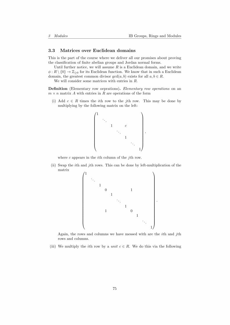
3 Modules IB Groups, Rings and Modules
3.3 Matrices over Euclidean domains
This is the part of the course where we deliver all our promises about provingthe classification of finite abelian groups and Jordan normal forms.
Until further notice, we will assume R is a Euclidean domain, and we writeφ : R \ 0 → Z≥0 for its Euclidean function. We know that in such a Euclideandomain, the greatest common divisor gcd(a, b) exists for all a, b ∈ R.
We will consider some matrices with entries in R.
Definition (Elementary row oeprations). Elementary row operations on anm× n matrix A with entries in R are operations of the form
(i) Add c ∈ R times the ith row to the jth row. This may be done bymultiplying by the following matrix on the left:
1. . .
1 c. . .
1. . .
1
,
where c appears in the ith column of the jth row.
(ii) Swap the ith and jth rows. This can be done by left-multiplication of thematrix
1. . .
10 1
1. . .
11 0
1. . .
1
.
Again, the rows and columns we have messed with are the ith and jthrows and columns.
(iii) We multiply the ith row by a unit c ∈ R. We do this via the following
75
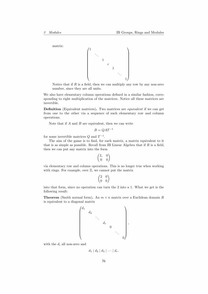
3 Modules IB Groups, Rings and Modules
matrix:
1. . .
1c
1. . .
1
Notice that if R is a field, then we can multiply any row by any non-zeronumber, since they are all units.
We also have elementary column operations defined in a similar fashion, corre-sponding to right multiplication of the matrices. Notice all these matrices areinvertible.
Definition (Equivalent matrices). Two matrices are equivalent if we can getfrom one to the other via a sequence of such elementary row and columnoperations.
Note that if A and B are equivalent, then we can write
B = QAT−1
for some invertible matrices Q and T−1.The aim of the game is to find, for each matrix, a matrix equivalent to it
that is as simple as possible. Recall from IB Linear Algebra that if R is a field,then we can put any matrix into the form(
Ir 00 0
)via elementary row and column operations. This is no longer true when workingwith rings. For example, over Z, we cannot put the matrix(
2 00 0
)into that form, since no operation can turn the 2 into a 1. What we get is thefollowing result:
Theorem (Smith normal form). An m× n matrix over a Euclidean domain Ris equivalent to a diagonal matrix
d1
d2
. . .
dr0
. . .
0
,
with the di all non-zero and
d1 | d2 | d3 | · · · | dr.
76
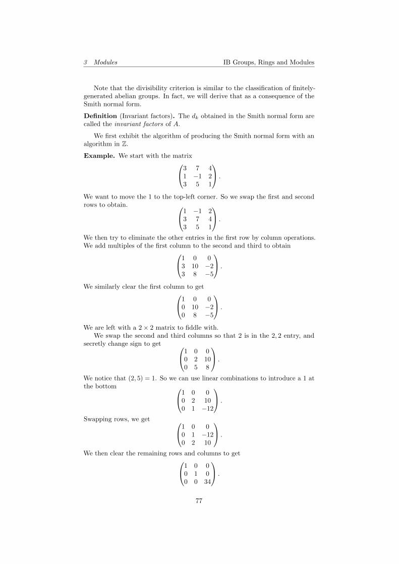
3 Modules IB Groups, Rings and Modules
Note that the divisibility criterion is similar to the classification of finitely-generated abelian groups. In fact, we will derive that as a consequence of theSmith normal form.
Definition (Invariant factors). The dk obtained in the Smith normal form arecalled the invariant factors of A.
We first exhibit the algorithm of producing the Smith normal form with analgorithm in Z.
Example. We start with the matrix3 7 41 −1 23 5 1
.
We want to move the 1 to the top-left corner. So we swap the first and secondrows to obtain. 1 −1 2
3 7 43 5 1
.
We then try to eliminate the other entries in the first row by column operations.We add multiples of the first column to the second and third to obtain1 0 0
3 10 −23 8 −5
.
We similarly clear the first column to get1 0 00 10 −20 8 −5
.
We are left with a 2× 2 matrix to fiddle with.We swap the second and third columns so that 2 is in the 2, 2 entry, and
secretly change sign to get 1 0 00 2 100 5 8
.
We notice that (2, 5) = 1. So we can use linear combinations to introduce a 1 atthe bottom 1 0 0
0 2 100 1 −12
.
Swapping rows, we get 1 0 00 1 −120 2 10
.
We then clear the remaining rows and columns to get1 0 00 1 00 0 34
.
77
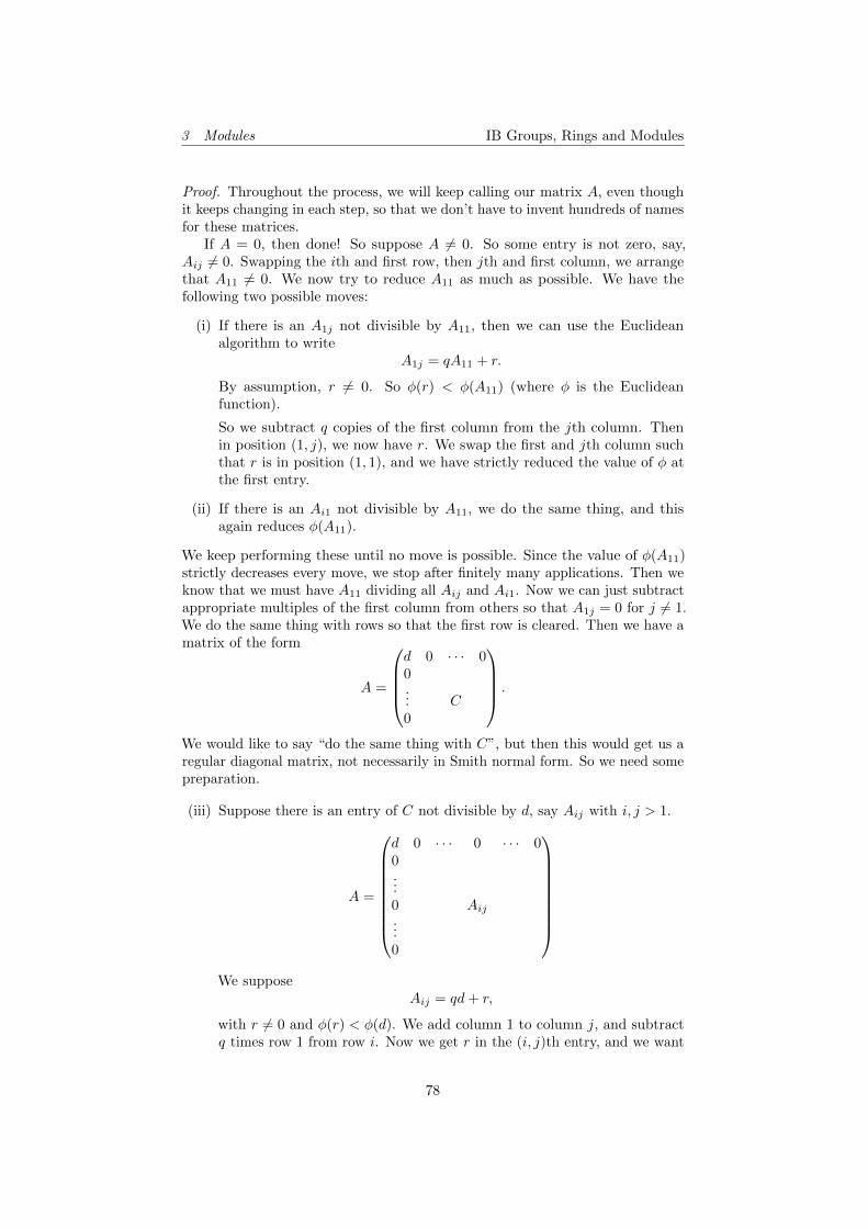
3 Modules IB Groups, Rings and Modules
Proof. Throughout the process, we will keep calling our matrix A, even thoughit keeps changing in each step, so that we don’t have to invent hundreds of namesfor these matrices.
If A = 0, then done! So suppose A 6= 0. So some entry is not zero, say,Aij 6= 0. Swapping the ith and first row, then jth and first column, we arrangethat A11 6= 0. We now try to reduce A11 as much as possible. We have thefollowing two possible moves:
(i) If there is an A1j not divisible by A11, then we can use the Euclideanalgorithm to write
A1j = qA11 + r.
By assumption, r 6= 0. So φ(r) < φ(A11) (where φ is the Euclideanfunction).
So we subtract q copies of the first column from the jth column. Thenin position (1, j), we now have r. We swap the first and jth column suchthat r is in position (1, 1), and we have strictly reduced the value of φ atthe first entry.
(ii) If there is an Ai1 not divisible by A11, we do the same thing, and thisagain reduces φ(A11).
We keep performing these until no move is possible. Since the value of φ(A11)strictly decreases every move, we stop after finitely many applications. Then weknow that we must have A11 dividing all Aij and Ai1. Now we can just subtractappropriate multiples of the first column from others so that A1j = 0 for j 6= 1.We do the same thing with rows so that the first row is cleared. Then we have amatrix of the form
A =
d 0 · · · 00... C0
.
We would like to say “do the same thing with C”, but then this would get us aregular diagonal matrix, not necessarily in Smith normal form. So we need somepreparation.
(iii) Suppose there is an entry of C not divisible by d, say Aij with i, j > 1.
A =
d 0 · · · 0 · · · 00...0 Aij...0
We suppose
Aij = qd+ r,
with r 6= 0 and φ(r) < φ(d). We add column 1 to column j, and subtractq times row 1 from row i. Now we get r in the (i, j)th entry, and we want
78
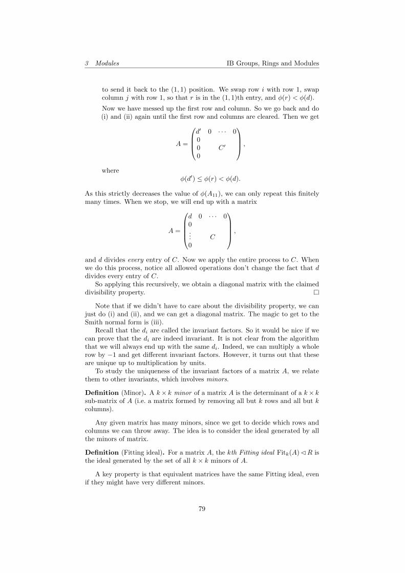
3 Modules IB Groups, Rings and Modules
to send it back to the (1, 1) position. We swap row i with row 1, swapcolumn j with row 1, so that r is in the (1, 1)th entry, and φ(r) < φ(d).
Now we have messed up the first row and column. So we go back and do(i) and (ii) again until the first row and columns are cleared. Then we get
A =
d′ 0 · · · 000 C ′
0
,
whereφ(d′) ≤ φ(r) < φ(d).
As this strictly decreases the value of φ(A11), we can only repeat this finitelymany times. When we stop, we will end up with a matrix
A =
d 0 · · · 00... C0
,
and d divides every entry of C. Now we apply the entire process to C. Whenwe do this process, notice all allowed operations don’t change the fact that ddivides every entry of C.
So applying this recursively, we obtain a diagonal matrix with the claimeddivisibility property.
Note that if we didn’t have to care about the divisibility property, we canjust do (i) and (ii), and we can get a diagonal matrix. The magic to get to theSmith normal form is (iii).
Recall that the di are called the invariant factors. So it would be nice if wecan prove that the di are indeed invariant. It is not clear from the algorithmthat we will always end up with the same di. Indeed, we can multiply a wholerow by −1 and get different invariant factors. However, it turns out that theseare unique up to multiplication by units.
To study the uniqueness of the invariant factors of a matrix A, we relatethem to other invariants, which involves minors.
Definition (Minor). A k× k minor of a matrix A is the determinant of a k× ksub-matrix of A (i.e. a matrix formed by removing all but k rows and all but kcolumns).
Any given matrix has many minors, since we get to decide which rows andcolumns we can throw away. The idea is to consider the ideal generated by allthe minors of matrix.
Definition (Fitting ideal). For a matrix A, the kth Fitting ideal Fitk(A)CR isthe ideal generated by the set of all k × k minors of A.
A key property is that equivalent matrices have the same Fitting ideal, evenif they might have very different minors.
79
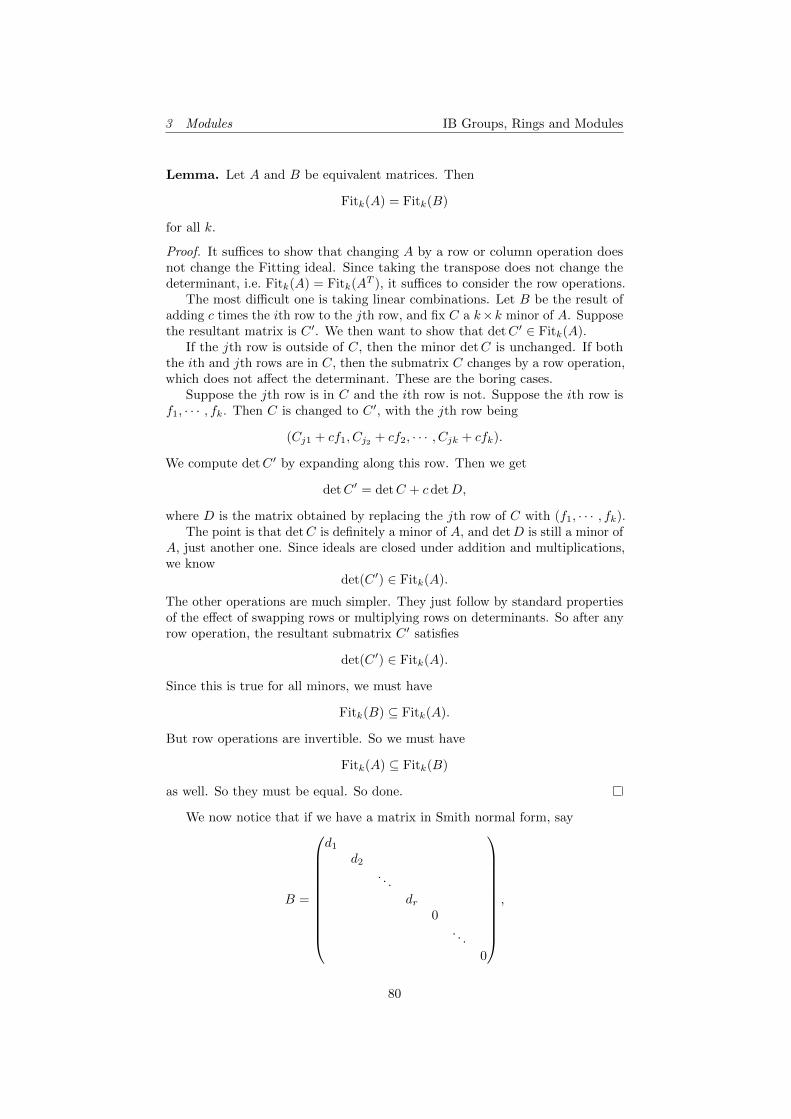
3 Modules IB Groups, Rings and Modules
Lemma. Let A and B be equivalent matrices. Then
Fitk(A) = Fitk(B)
for all k.
Proof. It suffices to show that changing A by a row or column operation doesnot change the Fitting ideal. Since taking the transpose does not change thedeterminant, i.e. Fitk(A) = Fitk(AT ), it suffices to consider the row operations.
The most difficult one is taking linear combinations. Let B be the result ofadding c times the ith row to the jth row, and fix C a k×k minor of A. Supposethe resultant matrix is C ′. We then want to show that detC ′ ∈ Fitk(A).
If the jth row is outside of C, then the minor detC is unchanged. If boththe ith and jth rows are in C, then the submatrix C changes by a row operation,which does not affect the determinant. These are the boring cases.
Suppose the jth row is in C and the ith row is not. Suppose the ith row isf1, · · · , fk. Then C is changed to C ′, with the jth row being
(Cj1 + cf1, Cj2 + cf2, · · · , Cjk + cfk).
We compute detC ′ by expanding along this row. Then we get
detC ′ = detC + cdetD,
where D is the matrix obtained by replacing the jth row of C with (f1, · · · , fk).The point is that detC is definitely a minor of A, and detD is still a minor of
A, just another one. Since ideals are closed under addition and multiplications,we know
det(C ′) ∈ Fitk(A).
The other operations are much simpler. They just follow by standard propertiesof the effect of swapping rows or multiplying rows on determinants. So after anyrow operation, the resultant submatrix C ′ satisfies
det(C ′) ∈ Fitk(A).
Since this is true for all minors, we must have
Fitk(B) ⊆ Fitk(A).
But row operations are invertible. So we must have
Fitk(A) ⊆ Fitk(B)
as well. So they must be equal. So done.
We now notice that if we have a matrix in Smith normal form, say
B =
d1
d2
. . .
dr0
. . .
0
,
80
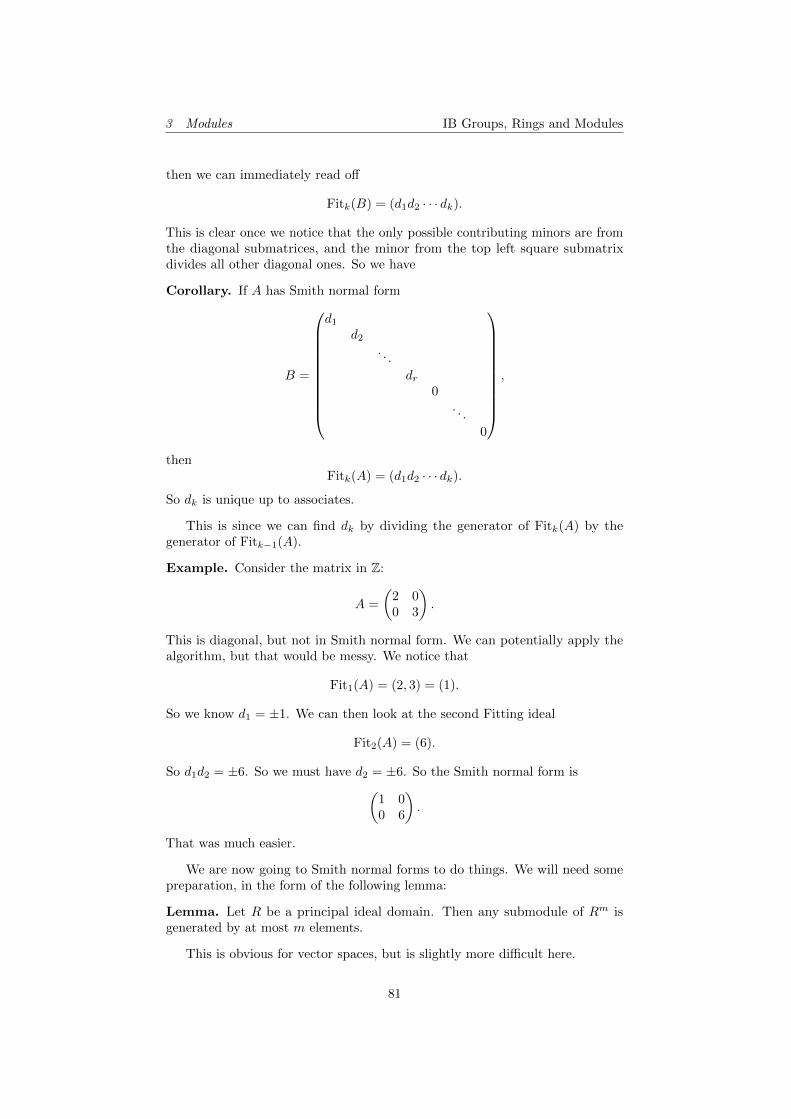
3 Modules IB Groups, Rings and Modules
then we can immediately read off
Fitk(B) = (d1d2 · · · dk).
This is clear once we notice that the only possible contributing minors are fromthe diagonal submatrices, and the minor from the top left square submatrixdivides all other diagonal ones. So we have
Corollary. If A has Smith normal form
B =
d1
d2
. . .
dr0
. . .
0
,
thenFitk(A) = (d1d2 · · · dk).
So dk is unique up to associates.
This is since we can find dk by dividing the generator of Fitk(A) by thegenerator of Fitk−1(A).
Example. Consider the matrix in Z:
A =
(2 00 3
).
This is diagonal, but not in Smith normal form. We can potentially apply thealgorithm, but that would be messy. We notice that
Fit1(A) = (2, 3) = (1).
So we know d1 = ±1. We can then look at the second Fitting ideal
Fit2(A) = (6).
So d1d2 = ±6. So we must have d2 = ±6. So the Smith normal form is(1 00 6
).
That was much easier.
We are now going to Smith normal forms to do things. We will need somepreparation, in the form of the following lemma:
Lemma. Let R be a principal ideal domain. Then any submodule of Rm isgenerated by at most m elements.
This is obvious for vector spaces, but is slightly more difficult here.
81
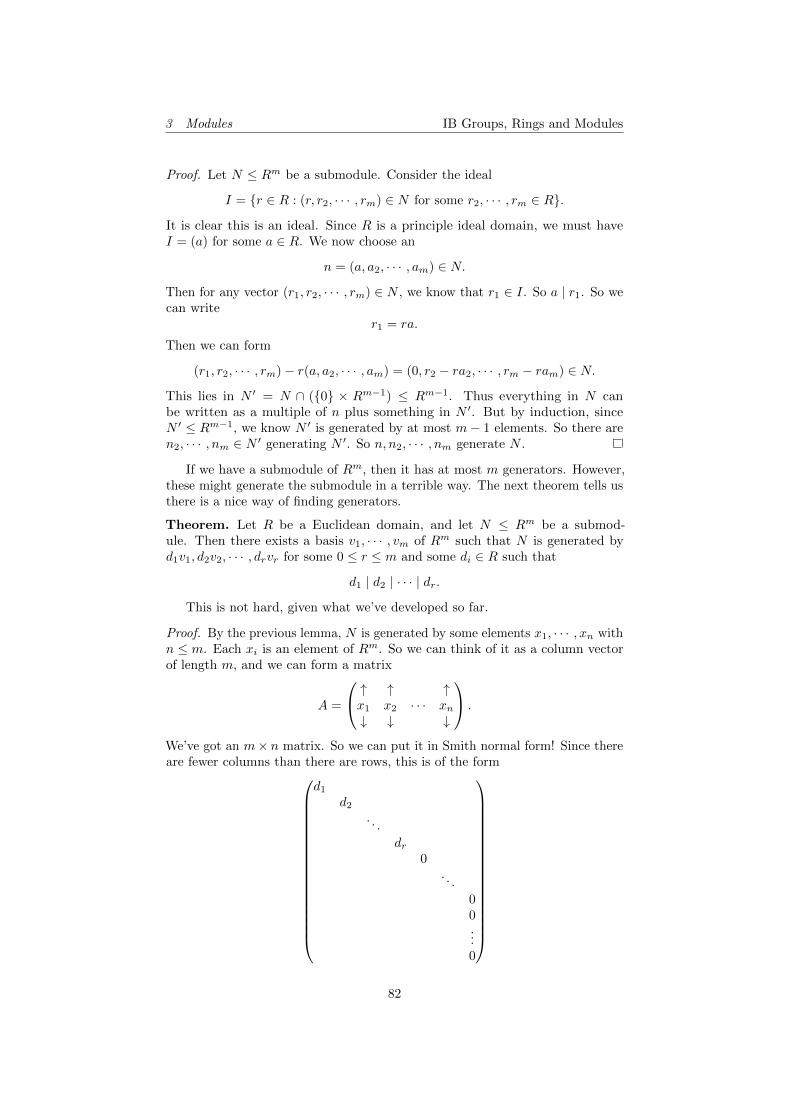
3 Modules IB Groups, Rings and Modules
Proof. Let N ≤ Rm be a submodule. Consider the ideal
I = r ∈ R : (r, r2, · · · , rm) ∈ N for some r2, · · · , rm ∈ R.
It is clear this is an ideal. Since R is a principle ideal domain, we must haveI = (a) for some a ∈ R. We now choose an
n = (a, a2, · · · , am) ∈ N.
Then for any vector (r1, r2, · · · , rm) ∈ N , we know that r1 ∈ I. So a | r1. So wecan write
r1 = ra.
Then we can form
(r1, r2, · · · , rm)− r(a, a2, · · · , am) = (0, r2 − ra2, · · · , rm − ram) ∈ N.
This lies in N ′ = N ∩ (0 × Rm−1) ≤ Rm−1. Thus everything in N canbe written as a multiple of n plus something in N ′. But by induction, sinceN ′ ≤ Rm−1, we know N ′ is generated by at most m− 1 elements. So there aren2, · · · , nm ∈ N ′ generating N ′. So n, n2, · · · , nm generate N .
If we have a submodule of Rm, then it has at most m generators. However,these might generate the submodule in a terrible way. The next theorem tells usthere is a nice way of finding generators.
Theorem. Let R be a Euclidean domain, and let N ≤ Rm be a submod-ule. Then there exists a basis v1, · · · , vm of Rm such that N is generated byd1v1, d2v2, · · · , drvr for some 0 ≤ r ≤ m and some di ∈ R such that
d1 | d2 | · · · | dr.
This is not hard, given what we’ve developed so far.
Proof. By the previous lemma, N is generated by some elements x1, · · · , xn withn ≤ m. Each xi is an element of Rm. So we can think of it as a column vectorof length m, and we can form a matrix
A =
↑ ↑ ↑x1 x2 · · · xn↓ ↓ ↓
.
We’ve got an m× n matrix. So we can put it in Smith normal form! Since thereare fewer columns than there are rows, this is of the form
d1
d2
. . .
dr0
. . .
00...0
82
3 Modules IB Groups, Rings and Modules
Recall that we got to the Smith normal form by row and column operations.Performing row operations is just changing the basis of Rm, while each columnoperation changes the generators of N .
So what this tells us is that there is a new basis v1, · · · , vm of Rm suchthat N is generated by d1v1, · · · , drvr. By definition of Smith normal form, thedivisibility condition holds.
Corollary. Let R be a Euclidean domain. A submodule of Rm is free of rankat most m. In other words, the submodule of a free module is free, and of asmaller (or equal) rank.
Proof. Let N ≤ Rm be a submodule. By the above, there is a basis v1, · · · , vnof Rm such that N is generated by d1v1, · · · , drvr for r ≤ m. So it is certainlygenerated by at mostm elements. So we only have to show that d1v1, · · · , drvr areindependent. But if they were linearly dependent, then so would be v1, · · · , vm.But v1, · · · , vn are a basis, hence independent. So d1v1, · · · , drvr generate Nfreely. So
N ∼= Rr.
Note that this is not true for all rings. For example, (2, X) C Z[X] is asubmodule of Z[X], but is not isomorphic to Z[X].
Theorem (Classification of finitely-generated modules over a Euclidean domain).Let R be a Euclidean domain, and M be a finitely generated R-module. Then
M ∼=R
(d1)⊕ R
(d1)⊕ · · · ⊕ R
(dr)⊕R⊕R⊕ · · · ⊕R
for some di 6= 0, andd1 | d2 | · · · | dr.
This is either a good or bad thing. If you are pessimistic, this says the worldof finitely generated modules is boring, since there are only these modules wealready know about. If you are optimistic, this tells you all finitely-generatedmodules are of this simple form, so we can prove things about them assumingthey look like this.
Proof. Since M is finitely-generated, there is a surjection φ : Rm →M . So bythe first isomorphism, we have
M ∼=Rm
kerφ.
Since kerφ is a submodule of Rm, by the previous theorem, there is a basisv1, · · · , vm of Rm such that kerφ is generated by d1v1, · · · , drvr for 0 ≤ r ≤ mand d1 | d2 | · · · | dr. So we know
M ∼=Rm
((d1, 0, · · · , 0), (0, d2, 0, · · · , 0), · · · , (0, · · · , 0, dr, 0, · · · , 0)).
This is justR
(d1)⊕ R
(d2)⊕ · · · ⊕ R
(dr)⊕R⊕ · · · ⊕R,
with m− r copies of R.
83
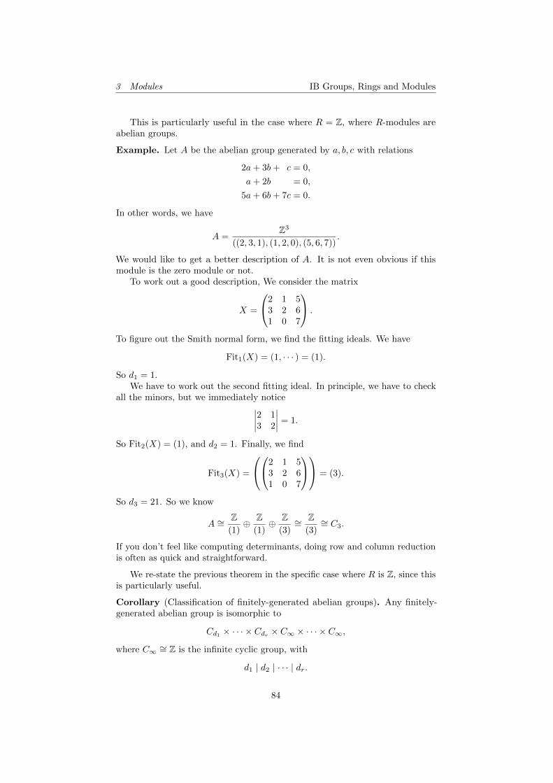
3 Modules IB Groups, Rings and Modules
This is particularly useful in the case where R = Z, where R-modules areabelian groups.
Example. Let A be the abelian group generated by a, b, c with relations
2a+ 3b+ c = 0,
a+ 2b = 0,
5a+ 6b+ 7c = 0.
In other words, we have
A =Z3
((2, 3, 1), (1, 2, 0), (5, 6, 7)).
We would like to get a better description of A. It is not even obvious if thismodule is the zero module or not.
To work out a good description, We consider the matrix
X =
2 1 53 2 61 0 7
.
To figure out the Smith normal form, we find the fitting ideals. We have
Fit1(X) = (1, · · · ) = (1).
So d1 = 1.We have to work out the second fitting ideal. In principle, we have to check
all the minors, but we immediately notice∣∣∣∣2 13 2
∣∣∣∣ = 1.
So Fit2(X) = (1), and d2 = 1. Finally, we find
Fit3(X) =
2 1 53 2 61 0 7
= (3).
So d3 = 21. So we know
A ∼=Z
(1)⊕ Z
(1)⊕ Z
(3)∼=
Z(3)∼= C3.
If you don’t feel like computing determinants, doing row and column reductionis often as quick and straightforward.
We re-state the previous theorem in the specific case where R is Z, since thisis particularly useful.
Corollary (Classification of finitely-generated abelian groups). Any finitely-generated abelian group is isomorphic to
Cd1 × · · · × Cdr × C∞ × · · · × C∞,
where C∞ ∼= Z is the infinite cyclic group, with
d1 | d2 | · · · | dr.
84
3 Modules IB Groups, Rings and Modules
Proof. Let R = Z, and apply the classification of finitely generated R-modules.
Note that if the group is finite, then there cannot be any C∞ factors. So itis just a product of finite cyclic groups.
Corollary. If A is a finite abelian group, then
A ∼= Cd1 × · · · × Cdr ,
withd1 | d2 | · · · | dr.
This is the result we stated at the beginning of the course.Recall that we were also to decompose a finite abelian group into products of
the form Cpk , where p is a prime, and we said it was just the Chinese remaindertheorem. This is again in general true, but we, again, need the Chinese remaindertheorem.
Lemma (Chinese remainder theorem). Let R be a Euclidean domain, anda, b ∈ R be such that gcd(a, b) = 1. Then
R
(ab)∼=
R
(a)× R
(b)
as R-modules.
The proof is just that of the Chinese remainder theorem written in ringlanguage.
Proof. Consider the R-module homomorphism
φ :R
(a)× R
(b)→ R
(ab)
by(r1 + (a), r2 + (b)) 7→ br1 + ar2 + (ab).
To show this is well-defined, suppose
(r1 + (a), r2 + (b)) = (r′1 + (a), r′2 + (b)).
Then
r1 = r′1 + xa
r2 = r′2 + yb.
So
br1 + ar2 + (ab) = br′1 + xab+ ar′2 + yab+ (ab) = br′1 + ar′2 + (ab).
So this is indeed well-defined. It is clear that this is a module map, by inspection.We now have to show it is surjective and injective. So far, we have not used
the hypothesis, that gcd(a, b) = 1. As we know gcd(a, b) = 1, by the Euclideanalgorithm, we can write
1 = ax+ by
85
3 Modules IB Groups, Rings and Modules
for some x, y ∈ R. So we have
φ(y + (a), x+ (b)) = by + ax+ (ab) = 1 + (ab).
So 1 ∈ imφ. Since this is an R-module map, we get
φ(r(y + (a), x+ (b))) = r · (1 + (ab)) = r + (ab).
The key fact is that R/(ab) as an R-module is generated by 1. Thus we know φis surjective.
Finally, we have to show it is injective, i.e. that the kernel is trivial. Suppose
φ(r1 + (a), r2 + (b)) = 0 + (ab).
Thenbr1 + ar2 ∈ (ab).
So we can writebr1 + ar2 = abx
for some x ∈ R. Since a | ar2 and a | abx, we know a | br1. Since a and b arecoprime, unique factorization implies a | r1. Similarly, we know b | r2.
(r1 + (a), r2 + (b)) = (0 + (a), 0 + (b)).
So the kernel is trivial.
Theorem (Prime decomposition theorem). Let R be a Euclidean domain, andM be a finitely-generated R-module. Then
M ∼= N1 ⊕N2 ⊕ · · · ⊕Nt,
where each Ni is either R or is R/(pn) for some prime p ∈ R and some n ≥ 1.
Proof. We already know
M ∼=R
(d1)⊕ · · · ⊕ R
(dr)⊕R⊕ · · · ⊕R.
So it suffices to show that each R/(d1) can be written in that form. We let
d = pn11 pn2
2 · · · pnkk
with pi distinct primes. So each pnii is coprime to each other. So by the lemmaiterated, we have
R
(d1)∼=
R
(pn11 )⊕ · · · ⊕ R
(pnkk ).
3.4 Modules over F[X] and normal forms for matrices
That was one promise delivered. We next want to consider the Jordan normalform. This is less straightforward, since considering V directly as an F modulewould not be too helpful (since that would just be pure linear algebra). Instead,we use the following trick:
86
3 Modules IB Groups, Rings and Modules
For a field F, the polynomial ring F[X] is a Euclidean domain, so the resultsof the last few sections apply. If V is a vector space on F, and α : V → V is alinear map, then we can make V into an F[X]-module via
F[X]× V → V
(f, v) 7→ (f(α))(v).
We write Vα for this F[X]-module.
Lemma. If V is a finite-dimensional vector space, then Vα is a finitely-generatedF[X]-module.
Proof. If v1, · · · ,vn generate V as an F-module, i.e. they span V as a vectorspace over F, then they also generate Vα as an F[X]-module, since F ≤ F[X].
Example. Suppose Vα ∼= F[X]/(Xr) as F[X]-modules. Then in particularthey are isomorphic as F-modules (since being a map of F-modules has fewerrequirements than being a map of F[X]-modules).
Under this bijection, the elements 1, X,X2, · · · , Xr−1 ∈ F[X]/(Xr) form avector space basis for Vα. Viewing F[X]/(Xr) as an F-vector space, the actionof X has the matrix
0 0 · · · 0 01 0 · · · 0 00 1 · · · 0 0...
.... . .
......
0 0 · · · 1 0
.
We also know that in Vα, the action of X is by definition the linear map α. Sounder this basis, α also has matrix
0 0 · · · 0 01 0 · · · 0 00 1 · · · 0 0...
.... . .
......
0 0 · · · 1 0
.
Example. Suppose
Vα ∼=F[X]
((X − λ)r)
for some λ ∈ F. Consider the new linear map
β = α− λ · id : V → V.
Then Vβ ∼= F[Y ]/(Y r), for Y = X − λ. So there is a basis for V so that β lookslike
0 0 · · · 0 01 0 · · · 0 00 1 · · · 0 0...
.... . .
......
0 0 · · · 1 0
.
87
3 Modules IB Groups, Rings and Modules
So we know α has matrix λ 0 · · · 0 01 λ · · · 0 00 1 · · · 0 0...
.... . .
......
0 0 · · · 1 λ
So it is a Jordan block (except the Jordan blocks are the other way round, withzeroes below the diagonal).
Example. Suppose Vα ∼= F[X]/(f) for some polynomial f , for
f = a0 + a1X + · · ·+ ar−1Xr−1 +Xr.
This has a basis 1, X,X2, · · · , Xr−1 as well, in which α is
c(f) =
0 0 · · · 0 −a0
1 0 · · · 0 −a1
0 1 · · · 0 −a2
......
. . ....
...0 0 · · · 1 −ar−1
.
We call this the companion matrix for the monic polynomial f .
These are different things that can possibly happen. Since we have alreadyclassified all finitely generated F[X] modules, this allows us to put matrices in arather nice form.
Theorem (Rational canonical form). Let α : V → V be a linear endomorphismof a finite-dimensional vector space over F, and Vα be the associated F[X]-module.Then
Vα ∼=F[X]
(f1)⊕ F[X]
(f2)⊕ · · · ⊕ F[X]
(fs),
with f1 | f2 | · · · | fs. Thus there is a basis for V in which the matrix for α isthe block diagonal
c(f1) 0 · · · 00 c(f2) · · · 0...
.... . .
...0 0 · · · c(fs)
This is the sort of theorem whose statement is longer than the proof.
Proof. We already know that Vα is a finitely-generated F[X]-module. By thestructure theorem of F[X]-modules, we know
Vα ∼=F[X]
(f1)⊕ F[X]
(f2)⊕ · · · ⊕ F[X]
(fs)⊕ 0.
We know there are no copies of F[X], since Vα = V is finite-dimensional overF, but F[X] is not. The divisibility criterion also follows from the structuretheorem. Then the form of the matrix is immediate.
88
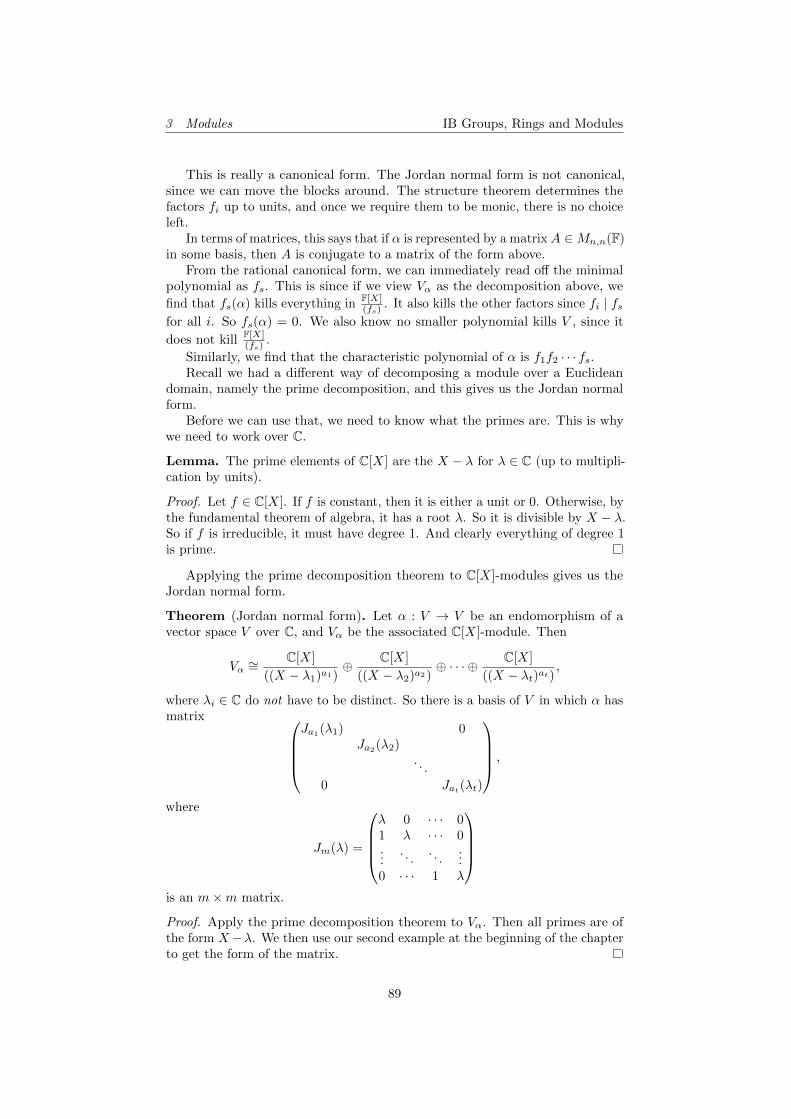
3 Modules IB Groups, Rings and Modules
This is really a canonical form. The Jordan normal form is not canonical,since we can move the blocks around. The structure theorem determines thefactors fi up to units, and once we require them to be monic, there is no choiceleft.
In terms of matrices, this says that if α is represented by a matrix A ∈Mn,n(F)in some basis, then A is conjugate to a matrix of the form above.
From the rational canonical form, we can immediately read off the minimalpolynomial as fs. This is since if we view Vα as the decomposition above, we
find that fs(α) kills everything in F[X](fs)
. It also kills the other factors since fi | fsfor all i. So fs(α) = 0. We also know no smaller polynomial kills V , since it
does not kill F[X](fs)
.
Similarly, we find that the characteristic polynomial of α is f1f2 · · · fs.Recall we had a different way of decomposing a module over a Euclidean
domain, namely the prime decomposition, and this gives us the Jordan normalform.
Before we can use that, we need to know what the primes are. This is whywe need to work over C.
Lemma. The prime elements of C[X] are the X − λ for λ ∈ C (up to multipli-cation by units).
Proof. Let f ∈ C[X]. If f is constant, then it is either a unit or 0. Otherwise, bythe fundamental theorem of algebra, it has a root λ. So it is divisible by X − λ.So if f is irreducible, it must have degree 1. And clearly everything of degree 1is prime.
Applying the prime decomposition theorem to C[X]-modules gives us theJordan normal form.
Theorem (Jordan normal form). Let α : V → V be an endomorphism of avector space V over C, and Vα be the associated C[X]-module. Then
Vα ∼=C[X]
((X − λ1)a1)⊕ C[X]
((X − λ2)a2)⊕ · · · ⊕ C[X]
((X − λt)at),
where λi ∈ C do not have to be distinct. So there is a basis of V in which α hasmatrix
Ja1(λ1) 0Ja2(λ2)
. . .
0 Jat(λt)
,
where
Jm(λ) =
λ 0 · · · 01 λ · · · 0...
. . .. . .
...0 · · · 1 λ
is an m×m matrix.
Proof. Apply the prime decomposition theorem to Vα. Then all primes are ofthe form X−λ. We then use our second example at the beginning of the chapterto get the form of the matrix.
89
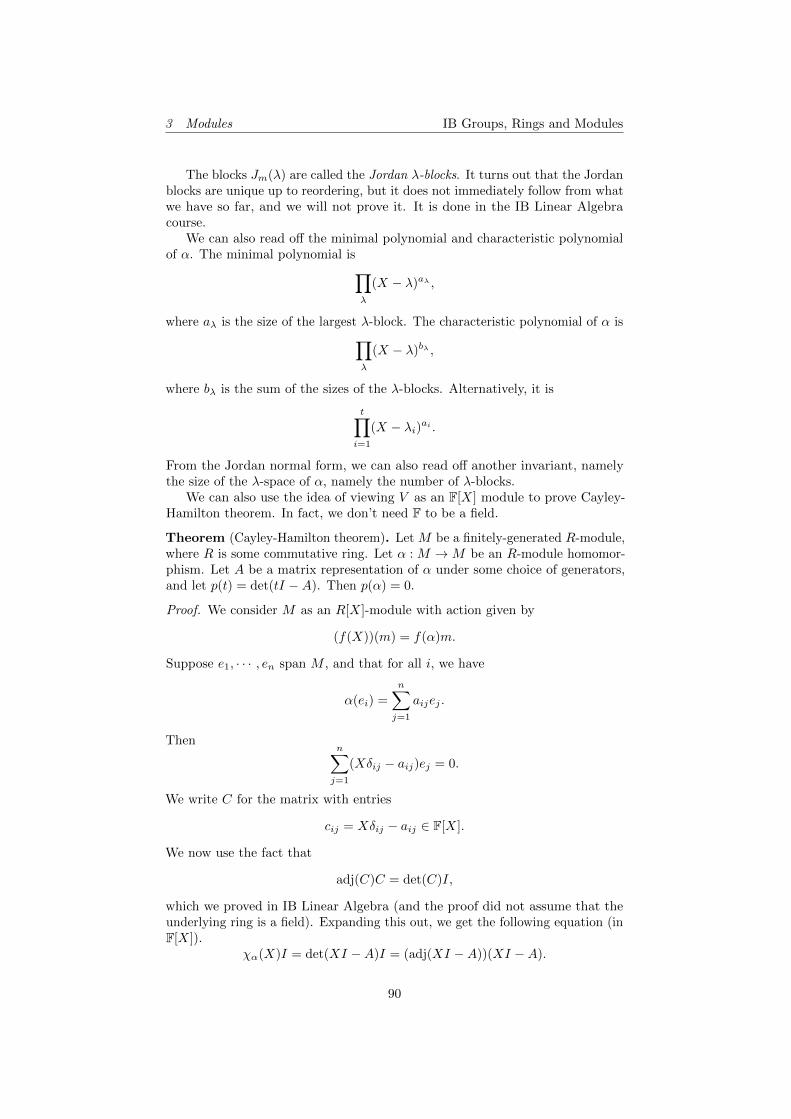
3 Modules IB Groups, Rings and Modules
The blocks Jm(λ) are called the Jordan λ-blocks. It turns out that the Jordanblocks are unique up to reordering, but it does not immediately follow from whatwe have so far, and we will not prove it. It is done in the IB Linear Algebracourse.
We can also read off the minimal polynomial and characteristic polynomialof α. The minimal polynomial is∏
λ
(X − λ)aλ ,
where aλ is the size of the largest λ-block. The characteristic polynomial of α is∏λ
(X − λ)bλ ,
where bλ is the sum of the sizes of the λ-blocks. Alternatively, it is
t∏i=1
(X − λi)ai .
From the Jordan normal form, we can also read off another invariant, namelythe size of the λ-space of α, namely the number of λ-blocks.
We can also use the idea of viewing V as an F[X] module to prove Cayley-Hamilton theorem. In fact, we don’t need F to be a field.
Theorem (Cayley-Hamilton theorem). Let M be a finitely-generated R-module,where R is some commutative ring. Let α : M →M be an R-module homomor-phism. Let A be a matrix representation of α under some choice of generators,and let p(t) = det(tI −A). Then p(α) = 0.
Proof. We consider M as an R[X]-module with action given by
(f(X))(m) = f(α)m.
Suppose e1, · · · , en span M , and that for all i, we have
α(ei) =
n∑j=1
aijej .
Thenn∑j=1
(Xδij − aij)ej = 0.
We write C for the matrix with entries
cij = Xδij − aij ∈ F[X].
We now use the fact that
adj(C)C = det(C)I,
which we proved in IB Linear Algebra (and the proof did not assume that theunderlying ring is a field). Expanding this out, we get the following equation (inF[X]).
χα(X)I = det(XI −A)I = (adj(XI −A))(XI −A).
90
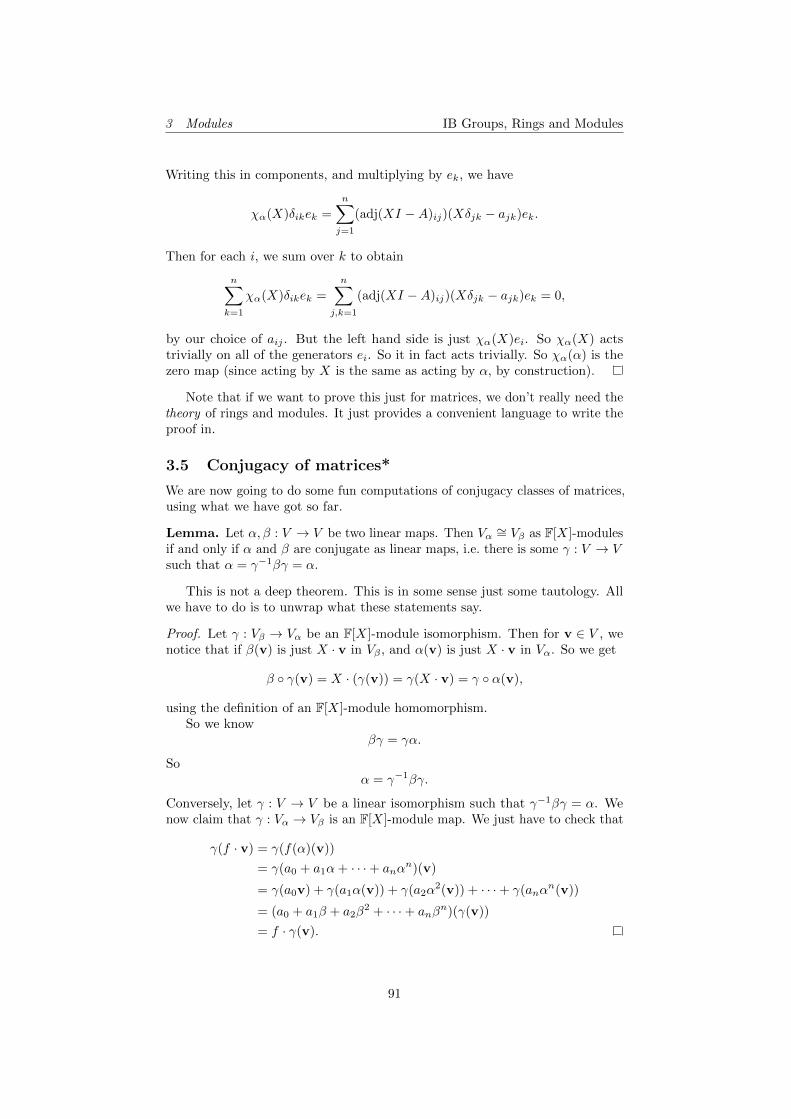
3 Modules IB Groups, Rings and Modules
Writing this in components, and multiplying by ek, we have
χα(X)δikek =
n∑j=1
(adj(XI −A)ij)(Xδjk − ajk)ek.
Then for each i, we sum over k to obtain
n∑k=1
χα(X)δikek =
n∑j,k=1
(adj(XI −A)ij)(Xδjk − ajk)ek = 0,
by our choice of aij . But the left hand side is just χα(X)ei. So χα(X) actstrivially on all of the generators ei. So it in fact acts trivially. So χα(α) is thezero map (since acting by X is the same as acting by α, by construction).
Note that if we want to prove this just for matrices, we don’t really need thetheory of rings and modules. It just provides a convenient language to write theproof in.
3.5 Conjugacy of matrices*
We are now going to do some fun computations of conjugacy classes of matrices,using what we have got so far.
Lemma. Let α, β : V → V be two linear maps. Then Vα ∼= Vβ as F[X]-modulesif and only if α and β are conjugate as linear maps, i.e. there is some γ : V → Vsuch that α = γ−1βγ = α.
This is not a deep theorem. This is in some sense just some tautology. Allwe have to do is to unwrap what these statements say.
Proof. Let γ : Vβ → Vα be an F[X]-module isomorphism. Then for v ∈ V , wenotice that if β(v) is just X · v in Vβ , and α(v) is just X · v in Vα. So we get
β γ(v) = X · (γ(v)) = γ(X · v) = γ α(v),
using the definition of an F[X]-module homomorphism.So we know
βγ = γα.
Soα = γ−1βγ.
Conversely, let γ : V → V be a linear isomorphism such that γ−1βγ = α. Wenow claim that γ : Vα → Vβ is an F[X]-module map. We just have to check that
γ(f · v) = γ(f(α)(v))
= γ(a0 + a1α+ · · ·+ anαn)(v)
= γ(a0v) + γ(a1α(v)) + γ(a2α2(v)) + · · ·+ γ(anα
n(v))
= (a0 + a1β + a2β2 + · · ·+ anβ
n)(γ(v))
= f · γ(v).
91
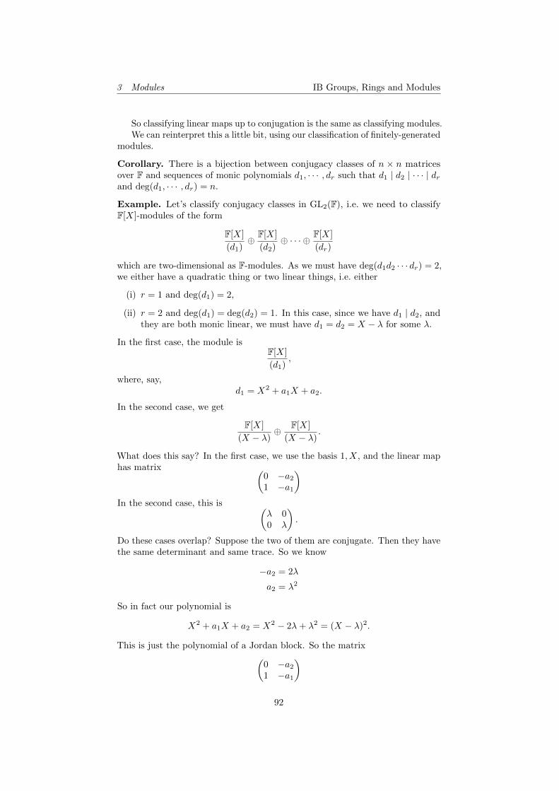
3 Modules IB Groups, Rings and Modules
So classifying linear maps up to conjugation is the same as classifying modules.We can reinterpret this a little bit, using our classification of finitely-generated
modules.
Corollary. There is a bijection between conjugacy classes of n × n matricesover F and sequences of monic polynomials d1, · · · , dr such that d1 | d2 | · · · | drand deg(d1, · · · , dr) = n.
Example. Let’s classify conjugacy classes in GL2(F), i.e. we need to classifyF[X]-modules of the form
F[X]
(d1)⊕ F[X]
(d2)⊕ · · · ⊕ F[X]
(dr)
which are two-dimensional as F-modules. As we must have deg(d1d2 · · · dr) = 2,we either have a quadratic thing or two linear things, i.e. either
(i) r = 1 and deg(d1) = 2,
(ii) r = 2 and deg(d1) = deg(d2) = 1. In this case, since we have d1 | d2, andthey are both monic linear, we must have d1 = d2 = X − λ for some λ.
In the first case, the module isF[X]
(d1),
where, say,d1 = X2 + a1X + a2.
In the second case, we get
F[X]
(X − λ)⊕ F[X]
(X − λ).
What does this say? In the first case, we use the basis 1, X, and the linear maphas matrix (
0 −a2
1 −a1
)In the second case, this is (
λ 00 λ
).
Do these cases overlap? Suppose the two of them are conjugate. Then they havethe same determinant and same trace. So we know
−a2 = 2λ
a2 = λ2
So in fact our polynomial is
X2 + a1X + a2 = X2 − 2λ+ λ2 = (X − λ)2.
This is just the polynomial of a Jordan block. So the matrix(0 −a2
1 −a1
)
92
3 Modules IB Groups, Rings and Modules
is conjugate to the Jordan block (λ 01 λ
),
but this is not conjugate to λI, e.g. by looking at eigenspaces. So these casesare disjoint.
Note that we have done more work that we really needed, since λI is invariantunder conjugation.
But the first case is not too satisfactory. We can further classify it as follows.If X2 + a1X + a2 is reducible, then it is
(X − λ)(X − µ)
for some µ, λ ∈ F. If λ = µ, then the matrix is conjugate to(λ 01 λ
)Otherwise, it is conjugate to (
λ 00 µ
).
In the case where X2 + a1X + a2 is irreducible, there is nothing we can doin general. However, we can look at some special scenarios and see if there isanything we can do.
Example. Consider GL2(Z/3). We want to classify its conjugacy classes. Bythe general theory, we know everything is conjugate to(
λ 00 µ
),
(λ 01 λ
),
(0 −a2
1 −a1
),
withX2 + a1X + a2
irreducible. So we need to figure out what the irreducibles are.A reasonable strategy is to guess. Given any quadratic, it is easy to see if it
is irreducible, since we can try to see if it has any roots, and there are just threethings to try. However, we can be a bit slightly more clever. We first count howmany irreducibles we are expecting, and then find that many of them.
There are 9 monic quadratic polynomials in total, since a1, a2 ∈ Z/3. Thereducibles are (X − λ)2 or (X − λ)(X − µ) with λ 6= µ. There are three of eachkind. So we have 6 reducible polynomials, and so 3 irreducible ones.
We can then check that
X2 + 1, X2 +X + 2, X2 + 2X + 2
are the irreducible polynomials. So every matrix in GL2(Z/3) is either congruentto (
0 −11 0
),
(0 −21 −1
),
(0 −21 −2
),
(λ 00 µ
),
(λ 01 λ
),
where λ 6= µ and λ, µ ∈ (Z/3)× (since the matrix has to be invertible). Thenumber of conjugacy classes of each type are 1, 1, 1, 3, 2. So there are 8 conjugacy
93
3 Modules IB Groups, Rings and Modules
classes. The first three classes have elements of order 4, 8, 8 respectively, bytrying. We notice that the identity matrix has order 1, and(
λ 00 µ
)has order 2 otherwise. Finally, for the last type, we have
ord
(1 01 1
)= 3, ord
(2 01 2
)= 6
Note that we also have
|GL2(Z/3)| = 48 = 24 · 3.Since there is no element of order 16, the Sylow 2-subgroup of GL2(Z/3) is notcyclic.
To construct the Sylow 2-subgroup, we might start with an element of order8, say
B =
(0 11 2
).
To make a subgroup of order 6, a sensible guess would be to take an element oforder 2, but that doesn’t work, since B4 will give you the element of order 2.Instead, we pick
A =
(0 21 0
).
We notice
A−1BA =
(0 12 0
)(0 11 2
)(0 21 0
)=
(1 20 2
)(0 21 0
)=
(2 22 0
)= B3.
So this is a bit like the dihedral group.We know that
〈B〉C 〈A,B〉.Also, we know |〈B〉| = 8. So if we can show that 〈B〉 has index 2 in 〈A,B〉, thenthis is the Sylow 2-subgroup. By the second isomorphism theorem, somethingwe have never used in our life, we know
〈A,B〉〈B〉
∼=〈A〉
〈A〉 ∩ 〈B〉.
We can list things out, and then find
〈A〉 ∩ 〈B〉 =
⟨(2 00 2
)⟩∼= C2.
We also know 〈A〉 ∼= C4. So we know
|〈A,B〉||〈B〉|
= 2.
So |〈A,B〉| = 16. So this is the Sylow 2-subgroup. in fact, it is
〈A,B | A4 = B8 = e,A−1BA = B3〉We call this the semi-dihedral group of order 16, because it is a bit like a dihedralgroup.
Note that finding this subgroup was purely guesswork. There is no methodto know that A and B are the right choices.
94
Index IB Groups, Rings and Modules
Index
An, 12Sn, 12Sym(X), 12sgn, 12p-group, 20
abelian group, 4ACC, 49algebraic integer, 60alternating group, 12annihilator, 69ascending chain condition, 49associates, 44automorphism group, 17
basis, 72
Cayley’s theorem, 15Cayley-Hamilton theorem, 90center, 18centralizer, 17characteristic, 38Chinese remainder theorem, 85classification of finite abelian
groups, 22classification of finitely-generated
abelian groups, 84classification of finitely-generated
modules over Euclideandomains, 83
commutative ring, 28conjugacy class, 17conjugation, 17content, 51coset, 5
degree, 30direct sum, 71division, 44
ED, 45Eisenstein’s criterion, 56elementary row operations, 75equivalent matrices, 76Euclidean algorithm for
polynomials, 35Euclidean domain, 45even permutation, 12
field, 29field of fractions, 40finitely generated module, 69finitely presented module, 73finitely-generated ideal, 62first isomorphism theorem, 8, 36, 68Fitting ideal, 79free module, 72freely generated, 71
Gauss’ lemma, 51Gaussian integers, 57gcd, 50generator of ideal, 33greatest common divisor, 50group, 4group action, 13
Hilbert basis theorem, 63homomorphism, 7, 31, 68
ideal, 32identity, 4image, 7, 31integral domain, 39invariant factors, 77inverse, 4irreducible, 44isomorphic, 8isomorphism, 8, 31, 68
Jordan normal form, 89
kernel, 7, 31
Lagrange’s theorem, 5Laurent polynomial, 31linear independence, 71
maximal ideal, 42minimal polynomial, 60minor, 79module, 66monic polynomial, 30
Noetherian ring, 49, 62normal subgroup, 6normalizer, 18
odd permutation, 12
95
Index IB Groups, Rings and Modules
orbit, 16orbit-stabilizer theorem, 17order, 5
permutation group, 13permutation representation, 14PID, 47polynomial, 30polynomial ring, 30power series, 30prime, 44prime decomposition theorem, 86prime ideal, 42primitive polynomial, 51principal ideal, 33principal ideal domain, 47product of rings, 29
quotient group, 6quotient ring, 34
rational canonical form, 88
relation, 73ring, 28
second isomorphism theorem, 9, 37,68
sign, 12simple group, 11Smith normal form, 76stabilizer, 16submodule, 67subring, 28Sylow theorem, 23symmetric group, 12
third isomorphism theorem, 10, 38,68
UFD, 48unique factorization domain, 48unit, 29, 43
zero divisor, 39
96


![GROTHENDIECK GROUPS OF ABELIAN GROUP RINGS › ~hwl › PUBLICATIONS › 1981a › art.pdf · Grofhendieck groups of obelian group rings 175 1. The Grothendieck group of R[l/n] In](https://static.fdocuments.net/doc/165x107/5f0f069c7e708231d4421e75/grothendieck-groups-of-abelian-group-a-hwl-a-publications-a-1981a-a-artpdf.jpg)


