Part 2: Basic Notions of Mathematical Logic - uni...
103
2. Basic Notions of Mathematical Logic 2-1 Part 2: Basic Notions of Mathematical Logic References: • Bergmann/Noll: Mathematische Logik mit Informatik-Anwendungen (in German). Springer, 1977. • Ebbinghaus/Flum/Thomas: Einf¨ uhrung in die mathematische Logik (in German). Spektrum Akademischer Verlag, 1996. • Tuschik/Wolter: Mathematische Logik, kurzgefasst (in German). Spektrum Akademischer Verlag, 2002. • Sch¨ oning: Logik f¨ ur Informatiker (in German). BI Verlag, 1992. • Chang/Lee: Symbolic Logic and Mechanical Theorem Proving. Academic Press, 1973. • Fitting: First Order Logic and Automated Theorem Proving. Springer, 1995, 2nd Edition. • Ulf Nilson, Jan Ma luszy´ nski: Logic, Programming, and Prolog (2nd Ed.). 1995, [http://www.ida.liu.se/˜ulfni/lpp] Stefan Brass: Datenbanken I Universit¨ at Halle, 2004
Transcript of Part 2: Basic Notions of Mathematical Logic - uni...

2. Basic Notions of Mathematical Logic 2-1
Part 2: Basic Notions ofMathematical Logic
References:• Bergmann/Noll: Mathematische Logik mit Informatik-Anwendungen (in German).
Springer, 1977.
• Ebbinghaus/Flum/Thomas: Einfuhrung in die mathematische Logik (in German).Spektrum Akademischer Verlag, 1996.
• Tuschik/Wolter: Mathematische Logik, kurzgefasst (in German).Spektrum Akademischer Verlag, 2002.
• Schoning: Logik fur Informatiker (in German).BI Verlag, 1992.
• Chang/Lee: Symbolic Logic and Mechanical Theorem Proving.Academic Press, 1973.
• Fitting: First Order Logic and Automated Theorem Proving.Springer, 1995, 2nd Edition.
• Ulf Nilson, Jan Ma luszynski: Logic, Programming, and Prolog (2nd Ed.).1995, [http://www.ida.liu.se/˜ulfni/lpp]
Stefan Brass: Datenbanken I Universitat Halle, 2004

2. Basic Notions of Mathematical Logic 2-2
Objectives
After completing this chapter, you should be able to:
• explain the basic notions: signature, interpretation,
variable assignment, term, formula, model, consi-
stent, implication.
• use some common equivalences to transform logical
formulas.
• write formulas for given specifications.
• check whether a formula is true in an interpretation,
• find models of a given formula (if consistent).
Stefan Brass: Datenbanken I Universitat Halle, 2004

2. Basic Notions of Mathematical Logic 2-3
Overview
1. Introduction, Motivation, History
'
&
$
%2. Signatures, Interpretations
3. Formulas, Models
4. Formulas in Databases
5. Implication, Equivalence
Stefan Brass: Datenbanken I Universitat Halle, 2004

2. Basic Notions of Mathematical Logic 2-4
Introduction, Motivation (1)
Important goals of mathematical logic are:
• to formalize the notion of a statement about a cer-
tain domain of discourse (logical formula),
• to precisely define the notions of logical implication
and proof,
• to find ways to mechanically check wether a state-
ment is logically implied by given statements.
As far as possible. It turned out that the task is in general undecidable.Actually, also the notion of decidability was developed by logicians.There was no computer science at that time (there was no computer).
Stefan Brass: Datenbanken I Universitat Halle, 2004
2. Basic Notions of Mathematical Logic 2-5
Introduction, Motivation (2)
Mathematical logic is applied in databases I:
• In general, the purpose of both, mathematical logic
and databases, is to
� formalize knowledge,
� work with this knowledge (process it).
• For instance, in order to talk about a domain of
discourse, symbols are needed.
� In logic, these are defined in a signature.
� In databases, they are defined in a DB schema.It should be no surprise that an important part of a databaseschema specifies a signature.
Stefan Brass: Datenbanken I Universitat Halle, 2004

2. Basic Notions of Mathematical Logic 2-6
Introduction, Motivation (3)
Mathematical logic is applied in databases II:
• In order to formalize logical implication, mathema-
tical logic had to study possible interpretations of
the symbols,
• i.e. possible situations in the domain of discourse
about which the logical formulas make statements.
• Database states also describe possible situations in
a certain part of the real world.
• Basically, logical interpretations and DB states are
the same (at least in the “model-theoretic view”).
Stefan Brass: Datenbanken I Universitat Halle, 2004

2. Basic Notions of Mathematical Logic 2-7
Introduction, Motivation (4)
Mathematical logic is applied in databases III:
• SQL queries are quite similar to formulas in ma-
thematical logic, and there are theoretical query
languages that are simply a version of logic.
• The idea is that
� a query is a logical formula with placeholders
(“free variables”),
� the database system then determines values for
these placeholders that make the formula true in
the given database state.
Stefan Brass: Datenbanken I Universitat Halle, 2004

2. Basic Notions of Mathematical Logic 2-8
Introduction, Motivation (5)
Why it makes sense to learn mathematical logic I:
• Logical formulas are simpler than SQL, and can
easily be formally studied.
• Important concepts of database queries can already
be learnt in this simpler, purer environment.
• Experience has shown that students often make
logical errors in SQL queries.
At least, when they are not specifically taught logic. It will be intere-sting to see whether the situation improves in this term.
Stefan Brass: Datenbanken I Universitat Halle, 2004

2. Basic Notions of Mathematical Logic 2-9
Introduction, Motivation (6)
Why it makes sense to learn mathematical logic II:
• SQL changes, and becomes more and more compli-
cated (standards: 1986, 1989, 1992, 1999, 2003).
At some point in the future, somebody will propose a drastically simp-ler language that can do the same. Datalog was already such a pro-posal, but somehow it was not yet successful. But look at Algol 68and PL/I, then followed by Pascal and C.
• There are new data models (e.g., XML) with new
query languages, and faster changes than SQL.
• At least some part of this course should still be
valid and useful in 30 years.
Stefan Brass: Datenbanken I Universitat Halle, 2004
2. Basic Notions of Mathematical Logic 2-10
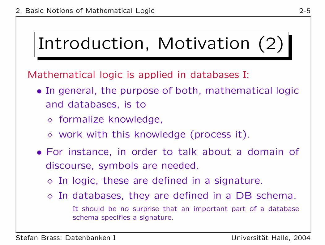
History of the Field (1)
∼322 BC Syllogisms [Aristoteles]∼300 BC Axioms of Geometry [Euklid]∼1700 Plan of Mathematical Logic [Leibniz]
1847 “Algebra of Logic” [Boole]1879 “Begriffsschrift” (Early Logical Formulas)
[Frege]∼1900 More natural formula syntax [Peano]
1910/13 Principia Mathematica (Collection offormal proofs) [Whitehead/Russel]
1930 Completeness Theorem [Godel/Herbrand]1936 Undecidability [Church/Turing]
Stefan Brass: Datenbanken I Universitat Halle, 2004

2. Basic Notions of Mathematical Logic 2-11
History of the Field (2)
1960 First Theorem Prover[Gilmore/Davis/Putnam]
1963 Resolution-Method for Theorem proving[Robinson]
∼1969 Question Answering Systems [Green et.al.]1970 Linear Resolution [Loveland/Luckham]1970 Relational Data Model [Codd]∼1973 Prolog [Colmerauer, Roussel, et.al.]
(Started as Theorem Prover for Natural Language Understanding)
(Compare with: Fortran 1954, Lisp 1962, Pascal 1970, Ada 1979)
1977 Conference “Logic and Databases”[Gallaire, Minker]
Stefan Brass: Datenbanken I Universitat Halle, 2004

2. Basic Notions of Mathematical Logic 2-12
Overview
1. Introduction, Motivation, History
2. Signatures, Interpretations
'
&
$
%3. Formulas, Models
4. Formulas in Databases
5. Implication, Equivalence
Stefan Brass: Datenbanken I Universitat Halle, 2004
2. Basic Notions of Mathematical Logic 2-13
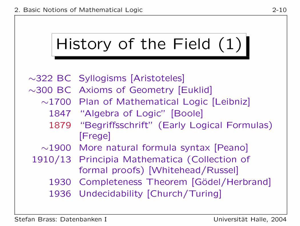
Alphabet (1)Definition:
• Let ALPH be some infinite, but enumerable set,
the elements of which are called symbols.Formulas will be words over ALPH, i.e. sequences of symbols.
• ALPH must contain at least the logical symbols,
i.e. LOG ⊆ ALPH, where
LOG = {(, ), , , >, ⊥, =, ¬, ∧, ∨, ←, →, ↔, ∀, ∃}.
• In addition, ALPH must contain an infinite subset
VARS ⊆ ALPH, the set of variables. This must be
disjoint to LOG (i.e. VARS ∩ LOG = ∅).Some authors consider variables as logical symbols.
Stefan Brass: Datenbanken I Universitat Halle, 2004

2. Basic Notions of Mathematical Logic 2-14
Alphabet (2)
• E.g., the alphabet might consist of
� the special logical symbols LOG,
� variables starting with an uppercase letter and
consisting otherwise of letters, digits, and “_”,
� identifiers starting with a lowercase letter and
consisting otherwise of letters, digits, and “_”.
• Note that words like “father” are considered as
symbols (elements of the alphabet).Compare with: lexical scanner vs. context-free parser in a compiler.
• In theory, the exact symbols are not important.
Stefan Brass: Datenbanken I Universitat Halle, 2004

2. Basic Notions of Mathematical Logic 2-15
Alphabet (3)
• If the special logical symbols are not available, use:
Symbol Alternative Alt2 Name
> true T
⊥ false F
¬ not ~ Negation∧ and & Conjunction∨ or | Disjunction← if <-
→ then ->
↔ iff <->
∃ exists E Existential Quantifier∀ forall A Universal Quantifier
Stefan Brass: Datenbanken I Universitat Halle, 2004
2. Basic Notions of Mathematical Logic 2-16
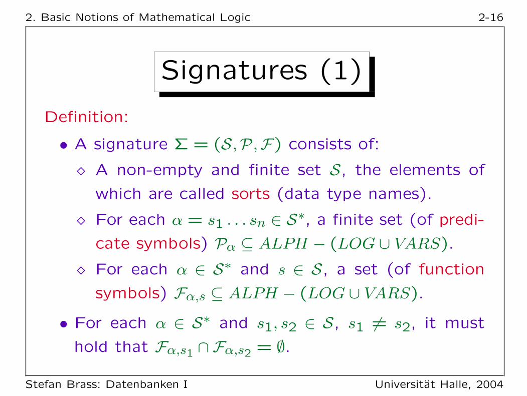
Signatures (1)
Definition:
• A signature Σ = (S,P,F) consists of:
� A non-empty and finite set S, the elements of
which are called sorts (data type names).
� For each α = s1 . . . sn ∈ S∗, a finite set (of predi-
cate symbols) Pα ⊆ ALPH − (LOG ∪ VARS).
� For each α ∈ S∗ and s ∈ S, a set (of function
symbols) Fα,s ⊆ ALPH − (LOG ∪ VARS).
• For each α ∈ S∗ and s1, s2 ∈ S, s1 6= s2, it must
hold that Fα,s1 ∩ Fα,s2 = ∅.
Stefan Brass: Datenbanken I Universitat Halle, 2004
2. Basic Notions of Mathematical Logic 2-17
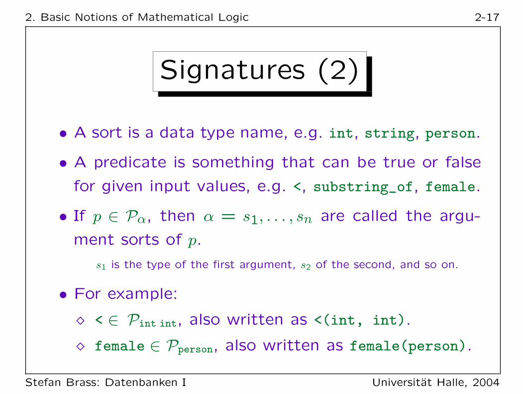
Signatures (2)
• A sort is a data type name, e.g. int, string, person.
• A predicate is something that can be true or false
for given input values, e.g. <, substring_of, female.
• If p ∈ Pα, then α = s1, . . . , sn are called the argu-
ment sorts of p.
s1 is the type of the first argument, s2 of the second, and so on.
• For example:
� < ∈ Pint int, also written as <(int, int).
� female ∈ Pperson, also written as female(person).
Stefan Brass: Datenbanken I Universitat Halle, 2004

2. Basic Notions of Mathematical Logic 2-18
Signatures (3)
• The number of argument sorts (length of α) is cal-
led the arity of a predicate symbol, e.g.:
� < is a predicate symbol of arity 2.
� female is a predicate symbol of arity 1.
• There are predicates of arity 0. They are called pro-
positional constants, or simply propositions. E.g.:
� the_sun_is_shining,
� i_am_working.
• The symbol ε is used to denote the empty sequence.
The set Pε contains the propositional constants.
Stefan Brass: Datenbanken I Universitat Halle, 2004

2. Basic Notions of Mathematical Logic 2-19
Signatures (4)
• The same symbol p can be element of several Pα
(overloaded predicate), e.g.
� < ∈ Pint int.
� < ∈ Pstring string
(lexicographic order, alphabetically before).
• This means that there are actually two different
predicates that have the same name.
The possibility of overloaded predicates is not very important, onecould also use two different names, e.g. lt_int and lt_string. Over-loaded predicates complicate the definitions a bit, therefore some au-thors exclude them. But they permit more natural formulations.
Stefan Brass: Datenbanken I Universitat Halle, 2004

2. Basic Notions of Mathematical Logic 2-20
Signatures (5)
• A function is something that returns a value for
given input values, e.g. +, age, first_name.
It is assumed here that functions are defined for all values of the inputtypes. This is not always true in reality, e.g. 5/0 is undefined, andtelefax_no(peter) might not exist. SQL uses a three-valued logic totreat null values (statements are not always true or false, they mightalso be undefined). One must always make a compromise between amodeling reality very exactly and finding a sufficiently simple model.
• A function symbol in Fα,s has argument sorts α and
result sort s, e.g.
� + ∈ Fint int, int, also written as +(int, int): int.
� age ∈ Fperson, int, also written as age(person): int.
Stefan Brass: Datenbanken I Universitat Halle, 2004

2. Basic Notions of Mathematical Logic 2-21
Signatures (6)
• A function with 0 arguments is called a constant.
• Examples of constants:
� 1 ∈ Fε,int, also written as 1: int.
� ’Ann’ ∈ Fε,string, also written as ’Ann’: string.
• For data types (e.g., int, string), it is usual that
every possible value can be denoted by a constant.
But in general, the set of values and the set of constants are diffe-rent concepts. For instance, it would be possible that there are noconstants of type person.
Stefan Brass: Datenbanken I Universitat Halle, 2004

2. Basic Notions of Mathematical Logic 2-22
Signatures (7)
• In summary, a signature specifies the application-
specific symbols that are used to talk about the
domain of discourse (a part of the real world that
is to be modeled in the database).
• The above definition is for a multi-sorted (typed)
logic. One can also use an unsorted logic.
Unsorted means really one-sorted. Then S is not needed, and P and Fare simply indexed by the arity. E.g. Prolog uses an unsorted logic.This is also common in textbooks about mathematical logic (the defi-nitions are a bit simpler). Since one can represent sorts as predicatesof arity 1, this is no real restriction (although a many-sorted logictreats some formulas as illegal, which are legal in one-sorted logic).
Stefan Brass: Datenbanken I Universitat Halle, 2004

2. Basic Notions of Mathematical Logic 2-23
Signatures (8)Example:
• S = {person, string}.
• F consists of
� constants of sort person, e.g. arno, birgit, chris.
� infinitely many constants of sort string, e.g. ’’,
’a’, ’b’, . . . , ’Arno’, . . .
� function symbols first_name(person): string and
last_name(person): string.
• P consists of
� a predicate married_to(person, person).
� predicates male(person) and female(person).
Stefan Brass: Datenbanken I Universitat Halle, 2004

2. Basic Notions of Mathematical Logic 2-24
Signatures (9)
Exercise:
• Define a signature for talking about
� Books (with authors, title, ISBN)It suffices to treat authors simply as a string. An advanced exercisewould be to model a list of strings (for books with several authors).
� Book reviews (with reviewer, text, stars).Every review is for exactly one book.
� “stars” can be none, one, two, three.
Stefan Brass: Datenbanken I Universitat Halle, 2004

2. Basic Notions of Mathematical Logic 2-25
Signatures (10)
Definition:
• A signature Σ′ = (S ′,P ′,F ′) is an extension of a
signature Σ = (S,P,F) iff
� S ⊆ S ′,
� for every α ∈ S∗:Pα ⊆ P ′α,
� for every α ∈ S∗:and s ∈ S: Fα,s ⊆ F ′α,s.
• I.e. an extension of Σ adds new symbols to Σ.
Stefan Brass: Datenbanken I Universitat Halle, 2004
2. Basic Notions of Mathematical Logic 2-26
Interpretations (1)
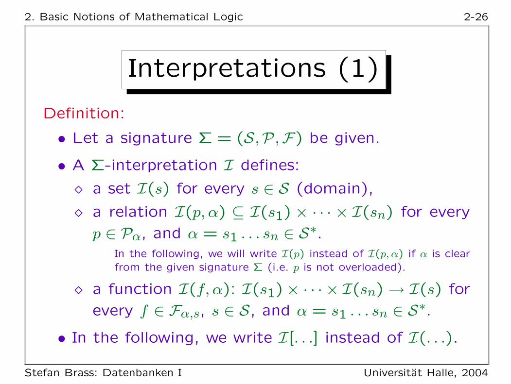
Definition:
• Let a signature Σ = (S,P,F) be given.
• A Σ-interpretation I defines:
� a set I(s) for every s ∈ S (domain),
� a relation I(p, α) ⊆ I(s1) × · · · × I(sn) for every
p ∈ Pα, and α = s1 . . . sn ∈ S∗.In the following, we will write I(p) instead of I(p, α) if α is clearfrom the given signature Σ (i.e. p is not overloaded).
� a function I(f, α): I(s1)× · · · × I(sn)→ I(s) for
every f ∈ Fα,s, s ∈ S, and α = s1 . . . sn ∈ S∗.
• In the following, we write I[. . .] instead of I(. . .).
Stefan Brass: Datenbanken I Universitat Halle, 2004

2. Basic Notions of Mathematical Logic 2-27
Interpretations (2)
Note:
• Empty domains cause certain problems, therefore
it is usual to exclude them.
Some equivalences do not hold if domains can be empty. For instan-ce, prenex normal form can only be reached under the assumptionthat domains are not empty. We will explicitly note where non-emptydomains are needed.
• But in databases, domains can be empty (e.g. a set
of persons when the database was just created).
This even causes problems in SQL when tuple variables are declaredover empty relations.
Stefan Brass: Datenbanken I Universitat Halle, 2004

2. Basic Notions of Mathematical Logic 2-28
Interpretations (3)
• The relation I[p] is also called the extension of p
(in I).
• Formally, predicate and relation are not the same,
but isomorphic notions.A predicate is a mapping to the set {true, false} of boolean values, arelation is a subset of a cartesian product ×.
• For instance, married_to(X, Y) is true in I if and only
if (X, Y) ∈ I[married_to].
• Another Example: (3, 5) ∈ I[<] means simply 3 < 5.In the following, the words “predicate symbol” and “relation symbol”are used interchangably.
Stefan Brass: Datenbanken I Universitat Halle, 2004

2. Basic Notions of Mathematical Logic 2-29
Interpretations (4)
Example (Interpretation for Signature on Slide 2-23):
• I[person] is the set of Arno, Birgit, and Chris.
• I[string] is the set of all strings, e.g. ’a’.
• I[arno] is Arno.
• For the string constants, I is the identity mapping.
• I[first_name] maps e.g. Arno to ’Arno’.
• I[last_name] maps all three persons to ’Schmidt’.
• I[married_to] = {(Birgit, Chris), (Chris, Birgit)}.
• I[male] = {(Arno), (Chris)}, I[female] = {(Birgit)}.
Stefan Brass: Datenbanken I Universitat Halle, 2004

2. Basic Notions of Mathematical Logic 2-30
Relational Databases (1)
• A DBMS defines a set of data types, such as strings
and numbers, together with constants, data type
functions (e.g. +) and predicates (e.g. <).
• For these, the DBMS defines names (in a signa-
ture Σ) and their meaning (in an interpretation I).
• For every value d ∈ I[s], there is at least one con-
stant c with I[c] = d.
I.e. all data values are named by constants. This is also known asthe domain closure assumption. It is important e.g. for printing datavalues that are results of queries. Note that in general there can beseveral constants mapped to the same data value, e.g. 0, 00, -0.
Stefan Brass: Datenbanken I Universitat Halle, 2004

2. Basic Notions of Mathematical Logic 2-31
Relational Databases (2)
• The DB schema in the relational model then adds
further predicate symbols (relation symbols).
These are the formal counterpart of the “tables” mentioned in theintroduction.
• The DB state interprets these by finite relations.
Whereas the interpretation of the data types is fixed and built in-to the DBMS, the interpretation of the additional predicate symbols(database relations) can be modified by insertions, deletions, and up-dates. But the database relations must have a finite extension. This isnatural because data type predicates are implemented by procedureswithin the DBMS, whereas the predicates from the database schemaare typically implemented as files of records.
Stefan Brass: Datenbanken I Universitat Halle, 2004

2. Basic Notions of Mathematical Logic 2-32
Relational Databases (3)
• Thus, the main restrictions of the relational model
are:
� No new sorts (types),
� No new function symbols and constants,
� New predicate symbols can only be interpreted
by finite relations.
• In addition, formulas are required to be “domain
independent” or “range restricted” (see below).I.e. not arbitrary formulas are permitted. This is necessary in orderto ensure that formulas can be evaluated in a given interpretation infinite time (although sorts like int are interpreted as infinite sets).
Stefan Brass: Datenbanken I Universitat Halle, 2004
2. Basic Notions of Mathematical Logic 2-33
Relational Databases (4)
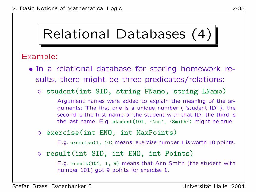
Example:
• In a relational database for storing homework re-
sults, there might be three predicates/relations:
� student(int SID, string FName, string LName)
Argument names were added to explain the meaning of the ar-guments: The first one is a unique number (“student ID”), thesecond is the first name of the student with that ID, the third isthe last name. E.g. student(101, ’Ann’, ’Smith’) might be true.
� exercise(int ENO, int MaxPoints)
E.g. exercise(1, 10) means: exercise number 1 is worth 10 points.
� result(int SID, int ENO, int Points)
E.g. result(101, 1, 9) means that Ann Smith (the student withnumber 101) got 9 points for exercise 1.
Stefan Brass: Datenbanken I Universitat Halle, 2004

2. Basic Notions of Mathematical Logic 2-34
Relational Databases (5)
• Here, we treat the “domain calculus” version of the
relational model.
There is also a “tuple calculus” version of the relational model,which is even more similar to SQL. The differences are not essen-tial, e.g. queries can automatically be converted in both directions.However, the definitions of the tuple calculus are a bit more com-plicated, because variables in tuple calculus range over entire tuples(table rows). Typically, database text books define both versions inseparate chapters as two different logical formalisms. However, onceone has understood one formalism (such as domain calculus), it isvery easy to learn the other one. Furthermore, the above formalismcan actually treat the part of tuple calculus that is used in SQL (itis like the entity-relationship model without relationships, see below):The difficult part are tuple variables that are not directly bound to adatabase relation (SQL forbids this and uses UNION instead).
Stefan Brass: Datenbanken I Universitat Halle, 2004

2. Basic Notions of Mathematical Logic 2-35
Entity-Relationship Model (1)
• In the Entity-Relationship-Model, the DB schema
can introduce
� new sorts (“entity types”),
� new functions of arity 1 from entity types to data
types (“attributes”),
� new predicates between entity types, possibly re-
stricted to arity 2 (“relationships”).
� new functions defined on the same entity types
as a relationship, returning a data type (“relati-
onship attributes”).
Stefan Brass: Datenbanken I Universitat Halle, 2004

2. Basic Notions of Mathematical Logic 2-36
Entity-Relationship Model (2)
• The interpretation of the entity types (in the DB
state) must always be finite.
Thus, also attributes and relationships are finite.
• Relationship attribute functions must yield a fixed
dummy value if they are called for a combination
of input values for which the corresponding relati-
onship is false.
Queries should be written in such a way that the exact dummy valueis not important for the query result. E.g. if f is an attribute of therelationship p, a formula of the form p(X, Y )∧f(X, Y ) = Z would havethis property. For a really clean treatment of relationship attributes,the logic must be extended, but this seems not worth the effort.
Stefan Brass: Datenbanken I Universitat Halle, 2004

2. Basic Notions of Mathematical Logic 2-37
Entity-Relationship Model (3)
Example (Homework Points):
• Sorts: student and exercise.
• Functions:
� sid(student): int
� first_name(student): string
� last_name(student): string.
� eno(exercise): int
� maxpoints(exercise): int
• Predicate: solved(student, exercise).
Function: points(student, exercise): int
Stefan Brass: Datenbanken I Universitat Halle, 2004

2. Basic Notions of Mathematical Logic 2-38
Overview
1. Introduction, Motivation, History
2. Signatures, Interpretations
3. Formulas, Models
'
&
$
%4. Formulas in Databases
5. Implication, Equivalence
Stefan Brass: Datenbanken I Universitat Halle, 2004

2. Basic Notions of Mathematical Logic 2-39
Variable Declaration (1)
Definition:
• Let a signature Σ = (S,P,F) be given.
• A variable declaration for Σ is a partial mapping
ν: VARS → S (defined only for a finite subset of VARS).
Remark:
• The variable declaration is not part of the signature
because it is locally modified by quantifiers (see
below).
• The signature is fixed for the entire application, the
variable declaration changes even within a formula.
Stefan Brass: Datenbanken I Universitat Halle, 2004

2. Basic Notions of Mathematical Logic 2-40
Variable Declaration (2)
Example:
• A variable declaration simply defines which variables
are available and what are their sorts, e.g.
ν
Variable SortSID int
Points int
E exercise
Of course, each variable must have a unique sort.
• Variable declarations are also written in the form
ν = {SID/int, Points/int, E/exercise}.
Stefan Brass: Datenbanken I Universitat Halle, 2004

2. Basic Notions of Mathematical Logic 2-41
Variable Declaration (3)
Definition:
• Let ν be a variable declaration, X ∈ VARS, and
s ∈ S.
• Then we write ν〈X/s〉 for the modified variable de-
claration ν′ with
ν′(V ) :=
s if V = Xν(V ) otherwise.
Remark:
• Both is possible: ν might have been defined before
for X or it might be undefined.
Stefan Brass: Datenbanken I Universitat Halle, 2004

2. Basic Notions of Mathematical Logic 2-42
Terms (1)
• Terms are syntactic constructs that can be evalua-
ted to a value (a number, a string, an exercise).
• There are three kinds of terms:
� constants, e.g. 1, ’abc’, arno,
� variables, e.g. X,
� composed terms, consisting of a function symbol
applied to argument terms, e.g. last_name(arno).This can be nested to arbitrary depth.
• In programming languages, terms are also called
expressions.
Stefan Brass: Datenbanken I Universitat Halle, 2004

2. Basic Notions of Mathematical Logic 2-43
Terms (2)
Definition:
• Let a signature Σ = (S,P,F) and a variable decla-
ration ν for Σ be given.
• The set TEΣ,ν(s) of terms of sort s is recursively
defined as follows: (nothing else is a term):
� Every variable V ∈ VARS with ν(V ) = s is a term
of sort s (this of course requires that ν is defined for V ).
� Every constant c ∈ Fε,s is a term of sort s.
� If t1 is a term of sort s1, . . . , tn is a term of
sort sn, and f ∈ Fα,s with α = s1 . . . sn, n ≥ 1,
then f(t1, . . . , tn) is a term of sort s.
Stefan Brass: Datenbanken I Universitat Halle, 2004
2. Basic Notions of Mathematical Logic 2-44
Terms (3)
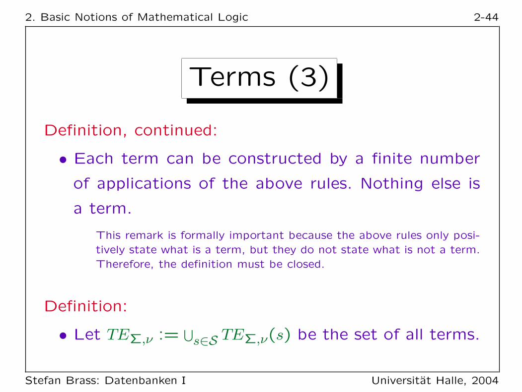
Definition, continued:
• Each term can be constructed by a finite number
of applications of the above rules. Nothing else is
a term.
This remark is formally important because the above rules only posi-tively state what is a term, but they do not state what is not a term.Therefore, the definition must be closed.
Definition:
• Let TEΣ,ν :=⋃
s∈S TEΣ,ν(s) be the set of all terms.
Stefan Brass: Datenbanken I Universitat Halle, 2004

2. Basic Notions of Mathematical Logic 2-45
Terms (4)
• Certain functions are also written as infix operators,
e.g. X+1 instead of the official notation +(X, 1).If one starts with this, one must also talk about precedence rules andusing parentheses as necessary.
• Functions of arity 1 can be written in dot-notation,
e.g. “X.first_name” instead of “first_name(X)”.
• Such “syntactic sugar” is useful in practice, but not
important for the theory of logic.In programming languages, there is sometimes a distinction between“concrete syntax” and “abstract syntax” (the syntax tree).
• In the following, the above abbreviations are used.
Stefan Brass: Datenbanken I Universitat Halle, 2004

2. Basic Notions of Mathematical Logic 2-46
Terms (5)
• Terms can be visualized as operator trees (“||” is
in SQL the function for string concatenation):
X
first_name�
��
�
||��
������
||
’ ’@
@@
@
X
last_nameHH
HHHHHH
• Exercise: How could this term be written with “||”
as infix operator and using the dot-notation?
Stefan Brass: Datenbanken I Universitat Halle, 2004
2. Basic Notions of Mathematical Logic 2-47
Terms (6)
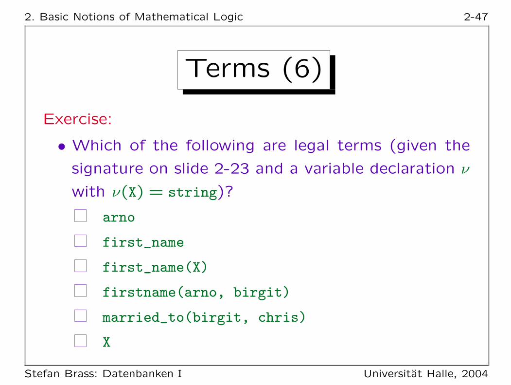
Exercise:
• Which of the following are legal terms (given the
signature on slide 2-23 and a variable declaration ν
with ν(X) = string)?
arno
first_name
first_name(X)
firstname(arno, birgit)
married_to(birgit, chris)
X
Stefan Brass: Datenbanken I Universitat Halle, 2004

2. Basic Notions of Mathematical Logic 2-48
Atomic Formulas (1)
• Formulas are syntactic expressions that can be eva-
luated to a truth value (true or false), e.g.
1 ≤ X ∧X ≤ 10.
• Atomic formulas are the basic building blocks of
such formulas (comparisons etc.).
• Atomic formulas can have the following forms:
� A predicate symbol applied to terms, e.g.
married_to(birgit, X).
� An equation, e.g. X = chris.
� The logical constants > (true) and ⊥ (false).
Stefan Brass: Datenbanken I Universitat Halle, 2004

2. Basic Notions of Mathematical Logic 2-49
Atomic Formulas (2)
Definition:
• Let a signature Σ = (S,P,F) and a variable decla-
ration ν for Σ be given.
• An atomic formula is an expression of one of the
following forms:
� p(t1, . . . , tn) with p ∈ Pα, α = s1 . . . sn ∈ S∗, and
ti ∈ TEΣ,ν(si) for i = 1, . . . , n.
� t1 = t2 with t1, t2 ∈ TEΣ,ν(s), s ∈ S.
� > and ⊥.
• Let AT Σ,ν be the set of atomic formulas for Σ, ν.
Stefan Brass: Datenbanken I Universitat Halle, 2004

2. Basic Notions of Mathematical Logic 2-50
Atomic Formulas (3)
Remarks:
• For some predicates, one traditionally uses infix no-
tation, e.g. X > 1 instead of >(X, 1).
Of course, we will use this common notation in the examples.
• For propositional constants, the parentheses can be
skipped, e.g. one can write p instead of p().
• Of course, it would be possible to treat “=” as a
normal predicate, and some authors do that.
However, the above definition ensures that at least the equality isavailable for all sorts, and below we will make sure it always has thestandard interpretation.
Stefan Brass: Datenbanken I Universitat Halle, 2004

2. Basic Notions of Mathematical Logic 2-51
Formulas (1)
Definition:
• Let a signature Σ = (S,P,F) and a variable decla-
ration ν for Σ be given.
• The sets FOΣ,ν of (Σ, ν)-formulas are defined re-
cursively as follows:
� Every atomic formula F ∈ AT Σ,ν is a formula.
� If F and G are formulas, so are (¬F ), (F ∧ G),
(F ∨G), (F ← G), (F → G), (F ↔ G).
� (∀ s X: F ) and (∃ s X: F ) are in FOΣ,ν if s ∈ S,
X ∈ VARS, and F is a ( Σ, ν〈X/s〉 )-formula.
� Nothing else is a formula.
Stefan Brass: Datenbanken I Universitat Halle, 2004

2. Basic Notions of Mathematical Logic 2-52
Formulas (2)
• The intuitive meaning of the formulas is as follows:
� ¬F : “Not F” (F is false).
� F ∧G: “F and G” (F and G are both true).
� F ∨G: “F or G” (at least one of F and G is true).
� F ← G: “F if G” (if G is true, F must be true).
� F → G: “if F , then G”
� F ↔ G: “F if and only if G”.
� ∀ s X: F : “for all X (of sort s), F is true”.
� ∃ s X: F : “there is an X (of sort s) such that F”.
Stefan Brass: Datenbanken I Universitat Halle, 2004

2. Basic Notions of Mathematical Logic 2-53
Formulas (3)
• Above, many parentheses are used in order to ensu-
re that formulas have a unique syntactic structure.
For the formal definition, this is a simple solution, but for writingformulas in practical applications, the syntax becomes clumsy.
• One uses the following rules to save parentheses:
� The outermost parentheses are never needed.
� ¬ binds strongest, then ∧, then ∨, then ←, →,
↔ (same binding strength), and last ∀, ∃.� Since ∧ and ∨ are associative, no parentheses are
required for e.g. F1 ∧ F2 ∧ F3.Note that → and ← are not associative.
Stefan Brass: Datenbanken I Universitat Halle, 2004

2. Basic Notions of Mathematical Logic 2-54
Formulas (4)
Formal Treatment of Binding Strengths:
• A level 0 formula is an atomic formula or a level 5
formula enclosed in parentheses.The level of a formula corresponds to the binding strength of its ou-termost operator (smallest number means highest binding strength).However, one can use a level i-formula like a level j-formula with j > i.In the opposite direction, parentheses are required.
• A level 1 formula is a level 0 formula or a formula
of the form ¬F with a level 1 formula F .
• A level 2 formula is a level 1 formula or a formula
of the form F1∧F2 with a level 2 formula F1 and a
level 1 formula F2.
Stefan Brass: Datenbanken I Universitat Halle, 2004

2. Basic Notions of Mathematical Logic 2-55
Formulas (5)
Formal Treatment of Binding Strengths, Continued:
• A level 3 formula is a level 2 formula or a formula
of the form F1∨F2 with a level 3 formula F1 and a
level 2 formula F2.
• A level 4 formula is a level 3 formula or a formula
of the form F1← F2, F1→ F2, F1↔ F2 with level 3
formulas F1 and F2.
• A level 5 formula is a level 4 formula or a formula of
the form ∀s X: F or ∃ s X: F with a level 5 formula F .
• A formula is a level 5 formula.
Stefan Brass: Datenbanken I Universitat Halle, 2004

2. Basic Notions of Mathematical Logic 2-56
Formulas (6)
Abbreviations for Quantifiers:
• When there is only one possible sort of a quanti-
fied variable, one can leave it out, i.e. write ∀X: F
instead of ∀ s X: F (and the same for ∃).
In most cases, there is indeed only one possible sort for a variable.
• If one quantifier immediately follows another quan-
tifier, one can leave out the colon.
E.g. write ∀X ∃Y : F instead of ∀X: ∃Y : F .
• Instead of a sequence of quantifiers of the same ty-
pe, e.g. ∀X1 . . . ∀Xn: F , one can write ∀X1, . . . , Xn: F .
Stefan Brass: Datenbanken I Universitat Halle, 2004

2. Basic Notions of Mathematical Logic 2-57
Formulas (7)
Abbreviation for Inequality:
• t1 6= t2 can be used as an abbreviation for ¬(t1 = t2).
Note:
• Some people say “formulae” instead of “formulas”.
Exercise:
• Given a signature with ≤ ∈ Pint int and 1, 10 ∈ Fε,int,
and a variable declaration with ν(X) = int.
• Is 1 ≤ X ≤ 10 a syntactically correct formula?
Stefan Brass: Datenbanken I Universitat Halle, 2004

2. Basic Notions of Mathematical Logic 2-58
Formulas (8)
Exercise:
• Which of the following are syntactically correct for-
mulas (given the signature on Slide 2-23)?
∀ X, Y: married_to(X, Y)→ married_to(Y, X)
∀ person P: ∨ male(P) ∨ female(P)
∀ person P: arno ∨ birgit ∨ chris
male(chris)
∀ string X: ∃ person X: married_to(birgit, X)
married_to(birgit, chris)∧ ∨ married_to(chris, birgit)
Stefan Brass: Datenbanken I Universitat Halle, 2004

2. Basic Notions of Mathematical Logic 2-59
Closed Formulas
Definition:
• Let a signature Σ be given.
• A closed formula (for Σ) is a (Σ, ν)-formula for the
empty variable declaration ν.I.e. the variable declaration that is everywhere undefined.
Exercise:
• Which of the following are closed formulas?
female(X) ∧ ∃ X: married_to(chris, X)
female(birgit) ∧ married_to(chris, birgit)
∃ X: married_to(X, Y)
Stefan Brass: Datenbanken I Universitat Halle, 2004

2. Basic Notions of Mathematical Logic 2-60
Variables in a Term
Definition:
• The function vars computes the set of variables
that occur in a given term t.
� If t is a constant c:
vars(t) := ∅.
� If t is a variable V :
vars(t) := {V }.
� If t has the form f(t1, . . . , tn):
vars(t) :=n⋃
i=1vars(ti).
Stefan Brass: Datenbanken I Universitat Halle, 2004

2. Basic Notions of Mathematical Logic 2-61
Free Variables in a FormulaDefinition:
• The function free computes the set of free variables
(not bound by a quantifier) in a formula F :
� If F is an atomic formula p(t1, . . . , tn) or t1 = t2:
free(F ) :=n⋃
i=1vars(ti).
� If F is > or ⊥: free(F ) := ∅.� If F has the form (¬G): free(F ) := free(G).
� If F has the form (G1 ∧G2), (G1 ∨G2), etc.:
free(F ) := free(G1) ∪ free(G2).
� If F has the form (∀ s X: G) or (∃ s X: G):
free(F ) := free(G)− {X}.
Stefan Brass: Datenbanken I Universitat Halle, 2004

2. Basic Notions of Mathematical Logic 2-62
Variable Assignment (1)
Definition:
• A variable assignment A for I and ν is a partial
mapping from VARS to⋃
s∈S I[s].
• It maps every variable V , for which ν is defined, to
a value from I[s], where s := ν(V ).
I.e. a variable assignment for I and ν defines values from I for thevariables that are declared in ν.
Remark:
• I.e. a variable assignment for I and ν defines values
from I for the variables that are declared in ν.
Stefan Brass: Datenbanken I Universitat Halle, 2004
2. Basic Notions of Mathematical Logic 2-63
Variable Assignment (2)
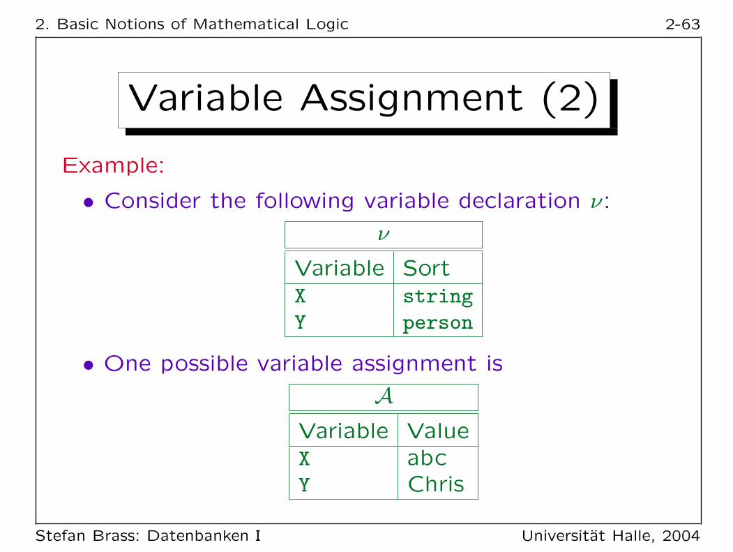
Example:
• Consider the following variable declaration ν:
ν
Variable SortX string
Y person
• One possible variable assignment is
AVariable ValueX abcY Chris
Stefan Brass: Datenbanken I Universitat Halle, 2004

2. Basic Notions of Mathematical Logic 2-64
Variable Assignment (3)
Definition:
• A〈X/d〉 denotes a variable assignment A′ that agrees
with A except that A′(X) = d.
Example:
• Given the variable declaration on the last slide,
A〈Y/Birgit〉 is:
A′
Variable ValueX abcY Birgit
Stefan Brass: Datenbanken I Universitat Halle, 2004

2. Basic Notions of Mathematical Logic 2-65
Value of a Term
Definition:
• Let a signature Σ, a variable declaration ν for Σ,
a Σ-interpretation I, and a variable assignment Afor (I, ν) be given.
• The value 〈I,A〉[t] of a term t ∈ TEΣ,ν is defined as
follows (recursion over the structure of the term):
� If t is a constant c, then 〈I,A〉[t] := I[c].
� If t is a variable V , then 〈I,A〉[t] := A(V ).
� If t has the form f(t1, . . . , tn), with ti of sort si:
〈I,A〉[t] := I[f, s1 . . . sn](〈I,A〉[t1], . . . , 〈I,A〉[tn]).
Stefan Brass: Datenbanken I Universitat Halle, 2004
2. Basic Notions of Mathematical Logic 2-66
Truth of a Formula (1)
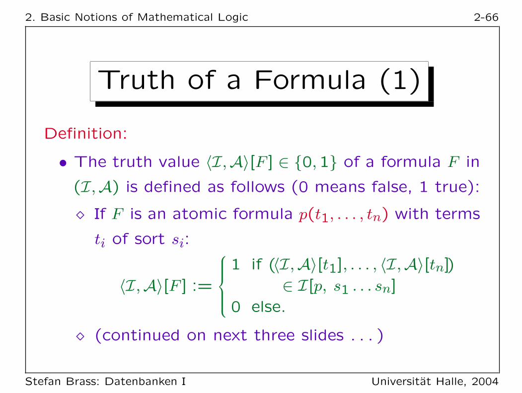
Definition:
• The truth value 〈I,A〉[F ] ∈ {0, 1} of a formula F in
(I,A) is defined as follows (0 means false, 1 true):
� If F is an atomic formula p(t1, . . . , tn) with terms
ti of sort si:
〈I,A〉[F ] :=
1 if (〈I,A〉[t1], . . . , 〈I,A〉[tn])
∈ I[p, s1 . . . sn]
0 else.
� (continued on next three slides . . . )
Stefan Brass: Datenbanken I Universitat Halle, 2004
2. Basic Notions of Mathematical Logic 2-67
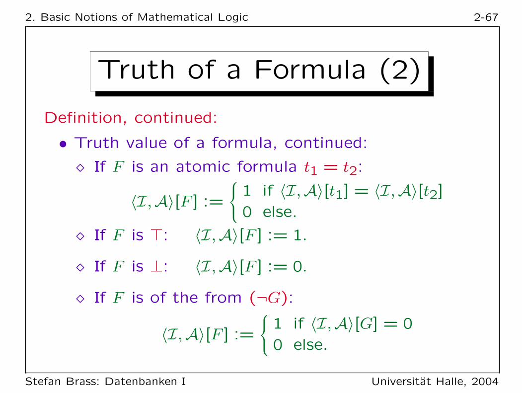
Truth of a Formula (2)
Definition, continued:
• Truth value of a formula, continued:
� If F is an atomic formula t1 = t2:
〈I,A〉[F ] :=
1 if 〈I,A〉[t1] = 〈I,A〉[t2]
0 else.
� If F is >: 〈I,A〉[F ] := 1.
� If F is ⊥: 〈I,A〉[F ] := 0.
� If F is of the from (¬G):
〈I,A〉[F ] :=
1 if 〈I,A〉[G] = 0
0 else.
Stefan Brass: Datenbanken I Universitat Halle, 2004

2. Basic Notions of Mathematical Logic 2-68
Truth of a Formula (3)
Definition, continued:
• Truth value of a formula, continued:
� If F is of the from (G1 ∧G2), (G1 ∨G2), etc.:
G1 G2 ∧ ∨ ← → ↔0 0 0 0 1 1 10 1 0 1 0 1 01 0 0 1 1 0 01 1 1 1 1 1 1
E.g. if 〈I,A〉[G1] = 1 and 〈I,A〉[G2] = 0 then 〈I,A〉[(G1 ∧G2)] = 0.
Stefan Brass: Datenbanken I Universitat Halle, 2004

2. Basic Notions of Mathematical Logic 2-69
Truth of a Formula (4)
Definition, continued:
• Truth value of a formula, continued:
� If F has the form (∀ s X: G):
〈I,A〉[F ] :=
1 if 〈I,A〈X/d〉〉[G] = 1
for all d ∈ I[s]0 else.
� If F has the form (∃ s X: G):
〈I,A〉[F ] :=
1 if 〈I,A〈X/d〉〉[G] = 1
for at least one d ∈ I[s]0 else.
Stefan Brass: Datenbanken I Universitat Halle, 2004

2. Basic Notions of Mathematical Logic 2-70
Model (1)
Definition:
• If 〈I,A〉[F ] = 1, one also writes 〈I,A〉 |= F .
• Let F be a (Σ, ν)-formula. A Σ-interpretation Iis a model of the formula F (written I |= F ) iff
〈I,A〉[F ] = 1 for all variable declarations A.I.e. free variables are treated as ∀-quantified. Of course, if F is aclosed formula, the variable declaration is not important.
• If I |= F , one says that I satisfies F .Or that F is true in I. The same for 〈I,A〉 |= F .
• A Σ-interpretation I is a model of a set Φ of Σ-
formulas, written I |= Φ, iff I |= F for all F ∈ Φ.
Stefan Brass: Datenbanken I Universitat Halle, 2004

2. Basic Notions of Mathematical Logic 2-71
Model (2)
Definition:
• A formula F or set of formulas Φ is called consistent
iff it has a model.
• A formula F is called satisfiable iff there is an inter-
pretation I and a variable declaration A such that
(I,A) |= F . Otherwise it is called unsatisfiable.
Sometimes I will say inconsistent when I really mean unsatisfiable.
• A (Σ, ν)-formula F is called a tautology iff for all Σ-
interpretations I and (Σ, ν)-variable assignments A:
(I,A) |= F .
Stefan Brass: Datenbanken I Universitat Halle, 2004

2. Basic Notions of Mathematical Logic 2-72
Model (3)Exercise:
• Consider the interpretation on Slide 2-29:
� I[person] = {Arno, Birgit, Chris}.� I[married_to] = {(Birgit, Chris), (Chris, Birgit)}.� I[male] = {(Arno), (Chris)},I[female] = {(Birgit)}.
• Which of the following formulas are true in I?
∀ person X: male(X)↔ ¬female(X)
∀ person X: male(X) ∨ ¬male(X)
∃ person X: female(X)∧¬∃ personY: married_to(X,Y)
∃ person X, person Y, person Z: X=Y ∧ Y=Z ∧ X 6=Z
Stefan Brass: Datenbanken I Universitat Halle, 2004

2. Basic Notions of Mathematical Logic 2-73
Overview
1. Introduction, Motivation, History
2. Signatures, Interpretations
3. Formulas, Models
4. Formulas in Databases
'
&
$
%5. Implication, Equivalence
Stefan Brass: Datenbanken I Universitat Halle, 2004

2. Basic Notions of Mathematical Logic 2-74
Formulas in Databases (1)
• As explained above, the DBMS defines a signa-
ture ΣD and an interpretation ID for the built-in
data types (string, int, . . . ).
• Then the database schema extends ΣD to the si-
gnature Σ of all symbols that can be used in, e.g.,
queries.
Every data model imposes certain restrictions for the kinds of newsymbols that can be introduced. For instance, in the classical re-lational model, the database schema can only define new predicatesymbols (relation symbols).
Stefan Brass: Datenbanken I Universitat Halle, 2004

2. Basic Notions of Mathematical Logic 2-75
Formulas in Databases (2)
• A database state is then an interpretation I for the
extended signature Σ.Of course, the system would explicitly store only the interpretation ofthe symbols of “Σ−ΣD”, because the interpretation of the symbols inΣD is already built into the DBMS and cannot be changed. Further-more, not arbitrary interpretations can be used as database states.The exact restrictions depend on the data model, but typically thenew symbols must have a finite interpretation.
• Formulas are used in databases as:
� Integrity constraints
� Queries
� Definitions of derived symbols (views).
Stefan Brass: Datenbanken I Universitat Halle, 2004

2. Basic Notions of Mathematical Logic 2-76
Integrity Constraints (1)
• Not all interpretations are reasonable DB states.
The purpose of the database is to model a certain part of the realworld. In the real world, certain restrictions exist. Therefore, interpre-tations that violate these restrictions should be excluded.
• For instance, in the real world, a person can only
be male or female, but not both. Therefore, the
following two formulas must be satisfied:
� ∀ person X: male(X) ∨ female(X)
� ∀ person X: ¬ male(X) ∨ ¬ female(X)
• These are examples of integrity constraints.
Stefan Brass: Datenbanken I Universitat Halle, 2004

2. Basic Notions of Mathematical Logic 2-77
Integrity Constraints (2)
• An integrity constraint is a closed formula.
The data model might not permit arbitrary formulas. Furthermore,the formulas must be domain independent (see below).
• A set of integrity constraints is specified as part of
the database schema.
• A database state (an interpretation) is called valid
iff it satisfies all integrity constraints.
In the following, we consider only valid database states. Therefore,we again speak only of “database state”.
Stefan Brass: Datenbanken I Universitat Halle, 2004

2. Basic Notions of Mathematical Logic 2-78
Integrity Constraints (3)
Keys I:
• Objects are often identified by unique data values
(numbers, names).
• For example, consider the signature on Slide 2-37.
There should never be two different objects of type
student with the same sid:
∀ student X, student Y: sid(X) = sid(Y) → X = Y
• Alternative, equivalent formulation:
¬∃ student X, student Y: sid(X) = sid(Y) ∧ X 6= Y
Stefan Brass: Datenbanken I Universitat Halle, 2004

2. Basic Notions of Mathematical Logic 2-79
Integrity Constraints (4)
Keys II:
• In the relational schema (Slide 2-33) a predicate of
arity 3 is used to store the student data.
• The first argument (SID) uniquely identifies the va-
lues of the other arguments (first name, last name):
∀ int ID, string F1, string F2, string L1, string L2:student(ID, F1, L1) ∧ student(ID, F2, L2) →
F1 = F2 ∧ L1 = L2
• Since keys are so common, each data model has
a special notation for them (one does not actually
have to write such formulas).
Stefan Brass: Datenbanken I Universitat Halle, 2004

2. Basic Notions of Mathematical Logic 2-80
Integrity Constraints (5)
Exercise:
• Consider the schema on Slide 2-33:
� student(int SID, string FName, string LName)
� exercise(int ENO, int MaxPoints)
� result(int SID, int ENO, int Points)
• Please write the following constraints:
� The Points in result are always non-negative.
� Each exercise number ENO in result appears also
in exercise (“no broken links”).
This is an example of a “foreign key constraint”.
Stefan Brass: Datenbanken I Universitat Halle, 2004

2. Basic Notions of Mathematical Logic 2-81
Queries (1)
• A query (Form A) is an expression of the form
{s1 X1, . . . , sn Xn | F},where F is a formula for the given DB signature Σ
and the variable declaration {X1/s1, . . . , Xn/sn}.Again, there might be restrictions for the possible formulas F , espe-cially the domain independence (see below).
• The query asks for all variable assignments A for
the result variables X1, . . . , Xn that make the for-
mula F true in the given database state I.In order to ensure that the variable assignment is printable, the sorts si
of the result variables typically must be data types.
Stefan Brass: Datenbanken I Universitat Halle, 2004

2. Basic Notions of Mathematical Logic 2-82
Queries (2)
Examples I:
• Consider the schema on Slide 2-33:
� student(int SID, string FName, string LName)
� exercise(int ENO, int MaxPoints)
� result(int SID, int ENO, int Points)
• Who got at least 8 points for Homework 1?
{string FName, string LName | ∃ int SID, int P:student(SID, FName, LName) ∧result(SID, 1, P) ∧ P ≥ 8}
Stefan Brass: Datenbanken I Universitat Halle, 2004

2. Basic Notions of Mathematical Logic 2-83
Queries (3)Examples II:
• Print all results for Ann Smith:
{int ENO, int Points | ∃ int SID:student(SID, ’Ann’, ’Smith’) ∧result(SID, ENO, Points)}
• Who has not yet submitted Exercise 2?
{string FName, string LName |∃ int SID: student(SID, FName, LName) ∧
¬ ∃ int P: result(SID, 2, P)}Exercise:
• Print students who have 10 points in Exercise 1
and 10 points in Exercise 2.
Stefan Brass: Datenbanken I Universitat Halle, 2004

2. Basic Notions of Mathematical Logic 2-84
Queries (4)
• A query (Form B) is an expression of the form
{t1, . . . , tk [s1 X1, . . . , sn Xn] | F},
where F is a formula and the ti are terms for the
given DB signature Σ and the variable declaration
{X1/s1, . . . , Xn/sn}.
• In this case, the DBMS will print the values 〈I,A〉[ti]of the terms ti for every variable assignments A for
the result variables X1, . . . , Xn such that 〈I,A〉 |= F .
This is especially convenient when the variables Xi range over sortsthat are otherwise not printable.
Stefan Brass: Datenbanken I Universitat Halle, 2004

2. Basic Notions of Mathematical Logic 2-85
Queries (5)
Example:
• Consider the schema on Slide 2-37:
� Sorts student, exercise.
� Functions first_name(student): string, . . .
� Predicate: solved(student, exercise).
Function: points(student, exercise): int
• Who got at least 8 points for Homework 1?
{S.first_name, S.last_name [student S] |∃ exercise E:
E.eno = 1 ∧ solved(S, E) ∧ points(S, E) ≥ 8}
Stefan Brass: Datenbanken I Universitat Halle, 2004

2. Basic Notions of Mathematical Logic 2-86
Queries (6)
• A query (Form C) is a closed formula F .
• The system prints “yes” if I |= F and “no” other-
wise.
Exercise:
• Suppose Form C is not available. Is it possible to
simulate it with Form A or Form B?
• Obviously, Form A is a special case of Form B:
{X1, . . . , Xn [s1 X1, . . . , sn Xn] | F}. Is it conversely
possible to simulate Form B with Form A?
Stefan Brass: Datenbanken I Universitat Halle, 2004

2. Basic Notions of Mathematical Logic 2-87
Domain Independence (1)
• One cannot use arbitrary formulas as queries. Some
formulas would generate an infinite answer:
{int SID | ¬student(SID, ’Ann’, ’Smith’}
• Other formulas would require that infinitely many
values are tried for quantified variables:
∃ int X, int Y, int Z: X ∗ X + Y ∗ Y = Z ∗ Z
• When a formula is domain-independent, it suffices
to consider only finitely many values for each va-
riable. Then the above problems do not occur.
Stefan Brass: Datenbanken I Universitat Halle, 2004

2. Basic Notions of Mathematical Logic 2-88
Domain Independence (2)
• A formula is domain independent iff for all possible
DB states (interpretations), it suffices to replace
variables that range over possibly infinite domains
by values that appear in any argument of the DB
relations, or as function value of a DB function, or
as variable-free term in the query.For a given interpretation I and formula F , the “active domain” isthe set of values that appear in database relations in I, as value inthe database sorts, as value of database functions, or as variable-freeterm (e.g. constant) in F . Domain independence means that (1) F
must be false if a value outside this set is inserted for a free variable.(2) For all subformulas ∃X: G, the formula G must be false if X hasa value outside the active domain. (3) For all subformulas ∀X: G, theformula G must be true if X has a value outside the active domain.
Stefan Brass: Datenbanken I Universitat Halle, 2004

2. Basic Notions of Mathematical Logic 2-89
Domain Independence (3)
• Since all database sorts, database relations, and da-
tabase functions are finite, queries can be evaluated
in finite time.
• For instance, the formula
∃ intX: X 6= 1
is not domain independent: The truth value de-
pends on other integers besides 1, but at least in
the empty database state there are no such values.The exact set of possible values (domain) is sometimes not known,only the set of values that appear in the database is known. Then it isgood if the truth value of a formula does not depend on the domain.
Stefan Brass: Datenbanken I Universitat Halle, 2004

2. Basic Notions of Mathematical Logic 2-90
Domain Independence (4)
• “Range restriction” is a syntactic constraint on for-
mulas that implies domain independence.
For every formula, one defines the set of restricted variables in posi-tive context and in negative context.
E.g. if F is an atomic formula p(t1, . . . , tn) with database relation p,then posres(F ) := {X ∈ VARS | ti is the variable X}, negres(F ) := ∅.For other atomic formulas, both sets are empty, except when F hasthe form X = t where t is variable-free or has a database function asoutermost function. Then posres(F ) := {X}.If F is ¬G, then posres(F ) := negres(G) and negres(F ) := posres(G).If F has the form G1 ∧G2, then posres(F ) := posres(G1) ∪ posres(G2)and negres(F ) := negres(G1) ∩ negres(G2). Etc.
A formula F is range restricted if free(F ) = posres(F ) and for everysubformula ∀X: G, it holds that X ∈ negres(G), and for every subfor-mula ∃X: G, it holds that X ∈ posres(G).
Stefan Brass: Datenbanken I Universitat Halle, 2004

2. Basic Notions of Mathematical Logic 2-91
Domain Independence (5)
• Basically, range striction requires that every varia-
ble is bound to a finite set of values.
E.g. by occurring in a database relation in positive context (unless itis universally quantified, then it must appear in negative context).
• Range restriction is decidable, whereas domain in-
dependence is in general undecidable.
E.g. ∃X: X 6= 1∧F would be domain independent if F is always false.The consistency of formulas (even range-restricted formulas) is un-decidable.
Nevertheless, range-restriction is sufficiently general: For instance,all relational algebra queries can be naturally translated into range-restricted formulas.
Stefan Brass: Datenbanken I Universitat Halle, 2004

2. Basic Notions of Mathematical Logic 2-92
Overview
1. Introduction, Motivation, History
2. Signatures, Interpretations
3. Formulas, Models
4. Formulas in Databases
5. Implication, Equivalence
'
&
$
%
Stefan Brass: Datenbanken I Universitat Halle, 2004
2. Basic Notions of Mathematical Logic 2-93
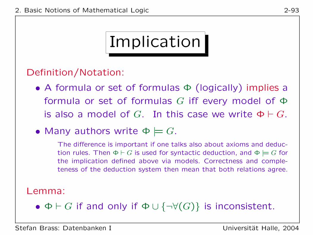
Implication
Definition/Notation:
• A formula or set of formulas Φ (logically) implies a
formula or set of formulas G iff every model of Φ
is also a model of G. In this case we write Φ ` G.
• Many authors write Φ |= G.The difference is important if one talks also about axioms and deduc-tion rules. Then Φ ` G is used for syntactic deduction, and Φ |= G forthe implication defined above via models. Correctness and comple-teness of the deduction system then mean that both relations agree.
Lemma:
• Φ ` G if and only if Φ ∪ {¬∀(G)} is inconsistent.
Stefan Brass: Datenbanken I Universitat Halle, 2004

2. Basic Notions of Mathematical Logic 2-94
Equivalence (1)
Definition/Lemma:
• Two Σ-formulas or sets of Σ-formulas F1 and F2
are equivalent iff they have the same models, i.e. for
every Σ-interpretation I:
I |= F1 ⇐⇒ I |= F2.
• F1 and F2 are equivalent iff F1 ` F2 and F2 ` F1.
Lemma:
• “Equivalence” of formulas is an equivalence relati-
on, i.e. it is reflexive, symmetric, and transitive.This also holds for strong equivalence defined on the next page.
Stefan Brass: Datenbanken I Universitat Halle, 2004

2. Basic Notions of Mathematical Logic 2-95
Equivalence (2)
Definition/Lemma:
• Two (Σ, ν)-formulas F1 and F2 are strongly equiva-
lent iff for every Σ-interpretation I and every (I, ν)-
variable declaration A:
(I,A) |= F1 ⇐⇒ (I,A) |= F2.
• Strong equivalence of F1 and F2 is written: F1 ≡ F2.
• Suppose that G1 results from G2 by replacing a
subformula F1 by F2 and let F1 and F2 be strongly
equivalent. Then G1 and G2 are strongly equivalent.
Stefan Brass: Datenbanken I Universitat Halle, 2004

2. Basic Notions of Mathematical Logic 2-96
Some Equivalences (1)
• Commutativity (for and, or, iff):
� F ∧G ≡ G ∧ F
� F ∨G ≡ G ∨ F
� F ↔ G ≡ G↔ F
• Associativity (for and, or, iff):
� F1 ∧ (F2 ∧ F3) ≡ (F1 ∧ F2) ∧ F3
� F1 ∨ (F2 ∨ F3) ≡ (F1 ∨ F2) ∨ F3
� F1↔ (F2↔ F3) ≡ (F1↔ F2)↔ F3
Stefan Brass: Datenbanken I Universitat Halle, 2004

2. Basic Notions of Mathematical Logic 2-97
Some Equivalences (2)
• Distribution Law:
� F ∧ (G1 ∨G2) ≡ (F ∧G1) ∨ (F ∧G2)
� F ∨ (G1 ∧G2) ≡ (F ∨G1) ∧ (F ∨G2)
• Double Negation:
� ¬(¬F ) ≡ F
• De Morgan’s Law:
� ¬(F ∧G) ≡ (¬F ) ∨ (¬G).
� ¬(F ∨G) ≡ (¬F ) ∧ (¬G).
Stefan Brass: Datenbanken I Universitat Halle, 2004

2. Basic Notions of Mathematical Logic 2-98
Some Equivalences (3)
• Replacements of Implication Operators:
� F ↔ G ≡ (F → G) ∧ (F ← G)
� F ← G ≡ G→ F
� F → G ≡ ¬F ∨G
� F ← G ≡ F ∨ ¬G
• Together with De Morgan’s Law this means that
e.g. {¬,∨} are sufficient, all other logical junctors
{∧,←,→,↔} can be expressed with them.
As we will see, also only one of the quantifiers is needed.
Stefan Brass: Datenbanken I Universitat Halle, 2004
2. Basic Notions of Mathematical Logic 2-99
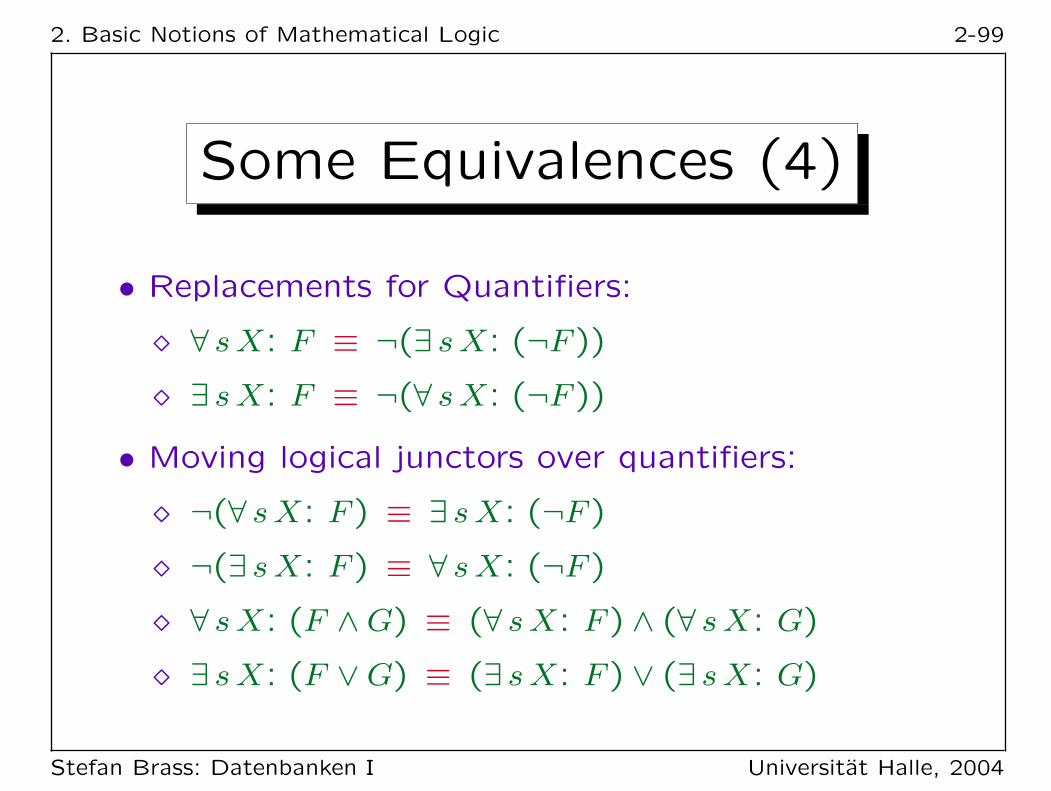
Some Equivalences (4)
• Replacements for Quantifiers:
� ∀ s X: F ≡ ¬(∃ s X: (¬F ))
� ∃ s X: F ≡ ¬(∀ s X: (¬F ))
• Moving logical junctors over quantifiers:
� ¬(∀ s X: F ) ≡ ∃ s X: (¬F )
� ¬(∃ s X: F ) ≡ ∀ s X: (¬F )
� ∀ s X: (F ∧G) ≡ (∀ s X: F ) ∧ (∀ s X: G)
� ∃ s X: (F ∨G) ≡ (∃ s X: F ) ∨ (∃ s X: G)
Stefan Brass: Datenbanken I Universitat Halle, 2004

2. Basic Notions of Mathematical Logic 2-100
Some Equivalences (5)
• Moving quantifiers: If X 6∈ free(F ):
� ∀ s X: (F ∨G) ≡ F ∨ (∀ s X: G)
� ∃ s X: (F ∧G) ≡ F ∧ (∃ s X: G)
If in addition I[s] cannot be empty:
� ∀ s X: (F ∧G) ≡ F ∧ (∀ s X: G)
� ∃ s X: (F ∨G) ≡ F ∨ (∃ s X: G)
• Removing unnecessary quantifiers:
If X 6∈ free(F ) and I[s] cannot be empty:
� ∀ s X: F ≡ F
� ∃ s X: F ≡ F
Stefan Brass: Datenbanken I Universitat Halle, 2004

2. Basic Notions of Mathematical Logic 2-101
Some Equivalences (6)
• Exchanging quantifiers: If X 6= Y :
� ∀ s1 X: (∀ s2 Y : F ) ≡ ∀ s2 Y : (∀ s1 X: F )
� ∃ s1 X: (∃ s2 Y : F ) ≡ ∃ s2 Y : (∃ s1 X: F )
Note that quantifiers of different type (∀ and ∃) cannot be ex-changed.
• Renaming bound variables: If Y 6∈ free(F ) and F ′
results from F by replacing every free occurrence
of X in F by Y :
� ∀ s X: F ≡ ∀ s Y : F ′
� ∃ s X: F ≡ ∃ s Y : F ′
Stefan Brass: Datenbanken I Universitat Halle, 2004
2. Basic Notions of Mathematical Logic 2-102
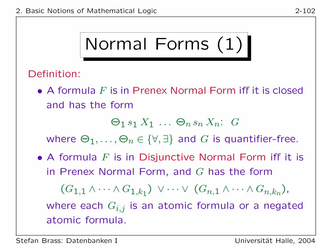
Normal Forms (1)
Definition:
• A formula F is in Prenex Normal Form iff it is closed
and has the form
Θ1 s1 X1 . . . Θn sn Xn: G
where Θ1, . . . , Θn ∈ {∀, ∃} and G is quantifier-free.
• A formula F is in Disjunctive Normal Form iff it is
in Prenex Normal Form, and G has the form
(G1,1 ∧ · · · ∧G1,k1) ∨ · · · ∨ (Gn,1 ∧ · · · ∧Gn,kn),
where each Gi,j is an atomic formula or a negated
atomic formula.
Stefan Brass: Datenbanken I Universitat Halle, 2004

2. Basic Notions of Mathematical Logic 2-103
Normal Forms (2)
Remark:
• Conjunctive Normal Form is like disjunctive normal
form, but G must have the form
(G1,1 ∨ · · · ∨G1,k1) ∧ · · · ∧ (Gn,1 ∨ · · · ∨Gn,kn).
Theorem:
• Under the assumption of non-empty domains, every
formula can be equivalently translated into prenex
normal form, disjunctive normal form, and conjunc-
tive normal form.
Stefan Brass: Datenbanken I Universitat Halle, 2004