0

Parent–Teacher Meetings and Student Outcomes:

Evidence from a Developing Country

Asad Islam* Department of Economics

Monash University Email: Asadul.islam@monash.edu

April 2018

Abstract We conduct a randomized field experiment involving regularly scheduled face-to-face meetings between teachers and parents over a period of two academic years. At each of these meetings, the teacher provided the parents with a report card and discussed the child’s academic progress. We find that the overall test scores of the students in the treatment schools increased by 0.26 SD in the first year, and 0.38 SD by the end of the second year. The program also resulted in improvements in both student attitudes and behavior, and teachers’ pedagogical practices. The intervention encouraged parents to spend more time assisting their children and monitoring their school work. The treatment effects are robust across parental, teacher, and school-level characteristics, and the findings indicate that programs for stimulating parent–teacher interactions are cost-effective, easy to implement, and easy to scale up.

JEL Classifications: C93, D83, I25, O12.

Keywords: parent-teacher meeting, educational outcomes, field experiments, Bangladesh

* I thank Sarah Baird, Abhijit Banerjee, Gaurav Datt, John Gibson, Sisira Jayasuriya, Victor Lavy, Wang-Sheng Lee, Wahiduddin Mahmud, Chau Nguyen, Berk Ozler, Steven Stillman, Russell Smyth, Choon Wang, Yves Zenou, and participants in seminars at the University of Urbana-Champaign, Australian National University, Queensland University of Technology, Royal Melbourne Institute of Technology, University of Sydney, LaTrobe University, North South University, BRAC, and Economic Research Group in Dhaka, as well as participants in the NEUDC 2016, Western Economic Association International conference, a development workshop at the University of Otago, and the Monash–Warwick workshop at Monash. Generous funding support from the International Growth Centre (IGC), AusAID (DFAT), and Monash University is gratefully acknowledged. This research would not have been possible without the hard work and due diligence of dedicated field staff members of the implementing NGO (Global Development Research Initiative). Kashem Khan and Jenarul Islam provided excellent support, coordinating all of the field work, while Zelin Wang provided excellent research assistance. The usual disclaimer applies.

1

1. Introduction

Parents can potentially play an important role in their children’s overall learning and education,

both at home and at school. Policy makers and educational experts have often advocated parents

being encouraged to be more involved in their children’s academic lives.1 Many children in

developing countries are first-generation students, and the parents of such children are often

unable to follow what happens at school (Banerjee and Duflo, 2006). Many of these parents are

not motivated to send their children to school or to encourage them to study.

This paper reports the results of a randomized field experiment involving a low-cost

intervention that examined whether students’ educational achievements can be improved by

increasing parental engagement through scheduled parent–teacher meetings. The experiment

involves monthly meetings that are similar to the parent–teacher interviews that occur in

schools in many developed countries. At each meeting, the teacher provided a report card that

contained information about a child’s academic performance.

Parental involvement with their children’s education can occur either at home (e.g., homework)

or at school (e.g., meetings, support, and/or volunteering). Although running regularly

scheduled parent–teacher meetings is a conventional practice in most developed countries, the

present study is the first to examine the effectiveness of encouraging active parental

involvement through one-on-one parent–teacher meetings in a developing country. The study

most similar to the present one was that undertaken in France by Avvisati, Gurgand, Guyon and

Maurin (2014), who conducted a field experiment in a relatively deprived educational district

of Paris which involved holding three general group meetings between parents and teachers

over an academic year so as to encourage parents to be more involved in their children’s

education. Avvisati et al. (2014) did not find any improvements in the test scores of the treated

students, except in French. However, they did find a 25% decline in truancy among low-income

families and an improvement in behavior among all students in the selected classes, including

those whose parents did not participate.2

1 In his 2009 address to the joint session of Congress, President Obama stated that “There is no program or policy that can substitute for a mother or father who will attend those parent–teacher conferences or help with the homework or turn off the TV, put away the video games, read to their child. Responsibility for our children’s education must begin at home.” 2 A number of recent studies in the US have demonstrated that an increase in parental involvement in their children’s learning is generally associated with better grades, test scores, and attendance, as well as with increased motivation and an easier transition to higher grades (see for example Bergman, 2016, on sending text messages to

2

We differ from Avvisati et al. (2014) in that we consider one-on-one meetings between parents

and teachers, which allowed frequent individualized communication. Our chosen method—

regular (monthly) face-to-face meetings between parents and teachers—is highly appropriate

for the conditions of developing countries because it is a low-cost, easy-to-implement method

that does not rely on written communication (which is important in situations where many

parents have poor literacy). We organized thirteen face-to-face meetings over the two academic

years 2011–2012. Like Avvisati et al. (2014), we implemented the intervention in poor areas,

but we chose remote rural communities. The intervention was not intended to help any

particular group, given that most of the children, whether high- or low-performing, were from

disadvantaged backgrounds, and it was impossible to know who may have had the most to gain

from such an intervention. The parents of these children have low incomes, are under-

represented in society, and tend to be less involved in their children’s educations.

In rural settings in Bangladesh, parents have limited contact with teachers, and have very little

knowledge about what is happening in their child’s school.3 The main objective of the meetings

was to ensure formal communications between parents and teachers so as to provide them with

the opportunity to meet and discuss the students’ academic progress. There are a few studies in

developing countries that have sought to provide parents with information. 4 For example, in

Pakistan, Andrabi, Das, and Khwaja (2017) used report cards to provide information to both

parents and schools about students’ tests scores. Nguyen (2008) provided parents with

information about returns to school in Madagascar. Dizon-Ross (2017) conducted information

parents when their children are absent, and Hastings and Weinstein, 2008, on informing parents of different public schools’ average test scores). 3 There are numerous reasons for the low level of parental involvement with school in rural and disadvantaged societies, such as men’s physical labor, women’s household chores and child-rearing duties, social norms, shyness (especially due to their lack of education), insufficient understanding of or information about the structure of the school system and the accepted communication channels, and a perception that teachers do not welcome such involvement. There is also a perception among teachers that parents are not interested in, or do not have the ability to help with, their children’s schooling. Informal communication is rare too, being limited to parents who are themselves very much motivated. The sorts of informal talks that usually occur at pick-up and/or drop-off times in schools in developed countries do not tend to happen in rural primary schools in developing countries because parents do not pick up or drop off their children; instead, students usually go to nearby schools by themselves. 4 A few recent studies have focused directly on the demand for schooling, such as training mothers to enhance their children’s learning (Banerji, Berry, and Shotland, 2017) and purchasing bicycles for girls to allow them to attend school (Muralidharan and Prakash, 2017). On the other hand, there have also been various interventions such as the traditional remedial educational interventions to improve the quality on the supply side through the provision of textbooks (Glewwe, Kremer, and Moulin, 2009), flipcharts (Glewwe, Kremer, Moulin, and Zitzewitz, 2004), school meals (Afridi, 2010), additional teachers (Duflo, Dupas, and Kremer, 2011; Muralidharan and Sundararaman, 2013), and classroom computers (Banerjee, Cole, Duflo, and Linden, 2007). These programs have generally been found to have positive effects on both attendance and test scores; however, most are expensive to implement (see Section 5.7 on the cost-effectiveness of our program). See Glewwe and Muralidharan (2016) for a review of the literature.

3

intervention and provided report cards to parents through surveyors in Malawi. As in the case

of the current study, the report cards contained information about the children’s academic

performances at school; however, there was no direct engagement between teachers and

parents. These interventions have all led to significant increases in student enrollments,

attendance and test scores, as well as in parental investment in education. The results of these

studies suggest that parents lack knowledge, but still have the ability to process new information

and change their decisions in a sophisticated manner.

On the other hand, studying India and Kenya respectively, Banerjee, Banerji, Duflo,

Glennerster and Khemani (2010) and Lieberman, Posner, and Tsai (2014) found the effects of

parents receiving information on students’ learning outcomes to be negligible. Their findings

indicate that the mere provision of information may not be sufficient to improve students’

performances if the parents have limited abilities to either help them at home or influence the

quality of their school education. However, once the provision of information is bundled with

a teaching intervention, Banerjee et al. (2010) found increases in test scores in a program that

used community volunteers as instructors, which suggests that involving teachers may be

another important element in impacting learning.

Parental involvement through frequent interactions with teachers, such as having parent–

teacher meetings in schools, may improve accountability and transparency, resulting in an

improvement in school services (e.g., Kremer, Brannen, and Glennerster, 2013; Mbiti, 2016).

Teacher accountability is likely to be improved by providing regular reports to parents, which

might change their pedagogical practices or efforts. Similarly, parents might be more engaged

with children at home if they met the teachers regularly to discuss their children’s performances,

homework, etc. 5 We examined these channels by conducting separate surveys for parents,

teachers, and students. We also examined changes in both the students’ behaviors and the

teachers’ perceptions of the students and their behaviors.

5 Parental efforts can also be crowded out by school resources, as parents may view their efforts and school quality as substitutes (Houtenville and Conway, 2008; Pop-Eleches and Urquiola, 2011). For example, Das et al. (2013) observed household substitution in spending in response to anticipated education grants in primary schools in India and Zambia, while Barrera-Osorio, Bertrand, Linden, and Perez-Calle (2011) found similar results in Colombia in response to a conditional cash transfer program. They found that parents took resources away from untreated siblings. On the other hand, Gelber and Isen (2013) observed a substantial increase in parental involvement in response to a government-funded preschool program.

4

Our primary focus was on examining the impact of such meetings on student test scores in

math, English, Bengali, and science, as well as on the students’ reading and writing skills and

general knowledge/intelligent quotient (GK/IQ) scores. Our main results can be summarized as

follows. First, parent–teacher meetings have a significant positive impact on children’s school

results. Students who were in the program for two successive years had increased their overall

test scores by 0.26 standard deviations (SD) at the end of year 1, and by 0.38 SD at the end of

year 2. They had also improved their reading and writing abilities, as well as their general

knowledge. Second, the short-term treatment effects are the greatest for high ability students,

whereas low ability students gain greater benefits from more frequent parent–teacher

interactions over time. Third, the treated students showed more positive attitudes and higher

aspirations, spent more time studying, and got more help from with studying family members.

Their behavior, as reported by both teachers and parents, also improved. Thus, we observed

increased parental involvement in their children’s studies. Fourth, we saw improvements in

absenteeism among both teachers and students. More importantly, we observed changes in the

teachers’ efforts in terms of pedagogical practices. Overall, our results suggest that the

interventions operated through both parents and teachers. We also found some positive spillover

effects on students in other grades of the treatment schools. Our results demonstrate that an

increased parental involvement in their children’s education through scheduled parent–teacher

meetings can be a cost-effective tool for enhancing student achievement.

2. Study Context and Background

We implemented the intervention in the rural areas of two southern districts (Khulna and

Satkhira) of Bangladesh. Most of the children are underprivileged and have parents from

relatively low socioeconomic backgrounds. In our study area, approximately a quarter of the

parents did not complete primary school, and more than 80% of families have no members who

have been educated past grade 10. Most mothers (80%) have had fewer than eight years of

education, and 98% work only in the home. Most fathers (90%) are engaged in agriculture, self-

employment activities, or day labor. The average household size in our sample is five, and the

average household monthly income is less than $150.

The school curriculum is the same in both the rural and urban areas of Bangladesh.6 Primary

schooling (grades 1–5) is compulsory, and incentives are offered to get children to come to

6 Some specialized and private schools in urban areas also offer additional extracurricular activities.

5

school; in particular, rural girls receive cash grants for attending school (Hahn et al., 2018). In

2015, the net enrollment rate in primary schools was 98% for girls and 97% for boys, while the

rate in secondary schools was 54% for girls and 45% for boys. Between 1990 and 2013, the

gender parity index (the school enrollment ratio of girls to boys) increased from 0.83 to 1.06 in

primary schools and from 0.51 to 1.08 in secondary schools. At the primary school level, the

teacher–student ratio is about 1:50 (BANBEIS, 2013).

Since the early 1990s, numerous policies, including the compulsory primary education law in

1991, have been enacted to ensure that all students attend, and complete, a primary education.

The government launched the Food for Education program in 1993 to support poor children in

completing primary schooling, and in 2002 this was replaced by the Primary Education Stipend

Project (PESP), which provides cash transfers to households with children attending schools in

poor areas. In addition, a variety of policies, including the elimination of official school fees

and the provision of free textbooks, have also been put in place to encourage school enrollment

(Hahn et al., 2018).

A single curriculum serves all students across the country. Education is exam-driven, because

the success of both teachers and schools is measured by their students’ results on exams, which

primarily demand the memorization and recall of content from textbooks (Holbrook, 2005). As

a consequence, teachers often encourage their students to perform rote learning and focus

largely on preparing students for their exams (Tapan, 2010). Students are generally promoted

to the next grade at the end of the academic year after passing the final exam. The exception is

at the end of grade 5, when students must face their first public examination, called the primary

school certificate (PSC) exam. The results of the PSC exam are used to determine students’

progression to secondary school.

However, education quality remains a major concern: nearly 50% of Bangladeshi students drop

out of primary school before completing grade 5, and only around 2% of children achieve the

prescribed competencies by the end of grade 5 (BANBEIS, 2013). Approximately 70% of

children who complete primary school nationwide are unable to read, write, or count properly.

Various factors contribute to this trend, including absenteeism by both teachers and students,

low classroom teaching time, and inflexibility in school hours. Studies have found that teacher

absenteeism hovers around 25%, with many teachers not instructing students even when present

at school. In addition, student absenteeism ranges from 40% to 67%, and the daily effective

6

instruction time in Bangladeshi primary schools is only 2.5 hours (UNESCO, 2010). Although

recent government initiatives have increased female enrollments, the academic performances

of girls are still significantly lower than those of boys (Hahn et al., 2016).

3.1 Intervention and Evaluation Design

3.1.1 The Intervention

The experiment involved scheduled parent–teacher meetings that were similar to the parent–

teacher conferences conducted in schools in many developed countries.7 The meetings were

conducted monthly over a period of two academic years, with the head teachers inviting the

students’ parents to these regular meetings to keep them informed about their children’s

progress in school. The teachers also provided the parents with written feedback by preparing

a report card for each student. In the particular context of Bangladesh, the parents felt the

meetings to be more important and significant if a document such as a report card was shown

to them at the meeting. The main purposes of the report card were to keep the information on

each child separately, and to encourage parents of the treatment schools to pay attention to the

information provided at the meetings. 8 The report card contained information about the

student’s test scores and the number of days the child had been absent from school in the

preceding month. See Appendix 3 for a sample report card. The parents did not take the report

card back home after the meeting, it was kept by the school.

The meetings were conducted by the class teachers. Each meeting between a parent and a

teacher was one-on-one and lasted about 15 minutes. Children did not attend the meetings. At

each meeting, the teacher explained how the child had performed on their regular class tests or

semester exams. They also provided oral guidelines for the parent, including how they could

help the child do their homework, how to check homework and class tests, the importance of

timely attendance at school, how to prepare students to go to school, and more. Report cards

were prepared separately for each child, with the guidelines being personalized rather than

scripted, and depending on the specific circumstances of each student (and the parents) as

perceived by class teachers. For example, if a child was not completing their homework, the

teachers would advise the child’s mother (or guardian) how she could help with completing the

7 For example, Australian schools have at least one parent–teacher interview session per academic term (there are four terms in a year), and there are also other formal and informal gatherings where parents and teachers can meet and share information about the children’s progress in school. 8 The schools do not keep any systematic student academic record, but only a student’s semester exam results (there are two such exams in a year) and class attendance. They keep no record of a student’s performance in the classroom, nor do they hold meetings with parents to provide any of this information.

7

homework, or how to get assistance if no one in the family was able to help. In some cases,

teachers offered extra help outside school hours if the parents were unable to help their children,

but the teachers never encouraged or advised parents to go for additional tutoring.9

As the parents come from a range of different socio-economic and educational backgrounds,

the teachers sometimes had to convey the same information to different parents in diverse ways.

In providing a parent with overall guidelines, the teachers focused mainly on the student’s

academic growth, but also took into account the student’s efforts in class, as well as their

attitudes and behaviors. They were encouraged to discuss any issues (e.g., behavioral issues)

related to students with their parents.

Note that report cards were prepared by teachers in both the treatment and control schools.

There was no additional assessment for students in the treatment schools, as the report cards

contained the same information in both the treatment and control schools. However, the parents

in the control schools did not receive the report cards at any point during the intervention. The

report cards in the control schools were prepared for the purposes of evaluation only, and no

parent–teacher meetings were organized by the teachers at the control schools.10 The report

cards were made available to parents only during the meetings in the treatment schools.

The intervention was implemented by a local NGO (Global Development Research Initiative

[GDRI]), with approval from the Bangladesh Department of Primary Education. Before the

intervention began, the researcher and representatives of the GDRI program held separate

meetings with the teachers in the treatment schools to inform them of the purpose of conducting

the meetings, show them how to prepare the report cards, and give them instructions on

providing parents with feedback about students.

Both the treatment and control schools received official letters from the ministry (department)

of primary education of Bangladesh, instructing them to help in conducting the research. Local

district and sub-district educational administrators also directed the schools to support the

9 This sometimes entailed working with a better performing classmate or talking to a guardian who could help. 10 Schools in Bangladesh, especially rural public schools, do not generally prepare report cards for students, as schools have no practice of issuing any regular information to parents. According to government guidelines for schools, parent–teacher meetings are supposed to be held a few times a year (though not monthly as we did), which also was confirmed by discussions with educational administrators in Bangladesh. In practice, though, they do not generally take place. However, such meetings are common in private schools in Bangladesh, as well as in select public schools in urban areas.

8

activities of the project. A separate letter explaining the basic objectives of the monthly parent–

teacher meetings was sent to the head teachers at the treatment schools, while the control

schools received only a letter instructing them to support the project’s activities. Neither the

treatment nor control school teachers received any instruction to change their pedagogical

practices or attitudes toward students.

Because the intervention required the school teachers to do additional work (discussing the

students’ progress with the parents and conducting additional tests), all teachers in both the

treatment and control schools were given a lump sum honorarium of US $25 for each of the

two years (the average monthly salary of a primary school teacher is $120–$160, depending on

their years of service).11 Each school typically had four or five teachers.

3.1.2 The Experimental Design

The field experiment was carried out in 76 government primary schools in rural areas in two

districts of Bangladesh. These schools were chosen randomly from a set of more than 200

schools in those regions, and are fairly typical of many parts of rural Bangladesh. The author

spent his childhood and attended both primary and secondary school in that area, and the area

was chosen because of the author’s local knowledge and contacts at schools, the NGO, and the

district level administration that facilitated the logistics for implementing the intervention.

A total of 40 schools were selected randomly for the treatment after baseline tests had been

conducted. The remaining 36 schools served as the control group throughout the two years of

intervention. The parent–teacher meetings began in the 2011 academic year; see Figure 1 for

the project timeline. The schools invited all parents to a short information session in early April

2011, at which the teachers explained the objectives of the monthly meetings. The schools then

set a date each month for the meetings, usually one week in advance, and the teachers sent out

verbal reminders or letters to the parents via the students before each meeting. After the initial

11 While the teachers in the control schools did not organize any meetings with parents, they still had to prepare the report cards and conduct the tests. Thus, the teachers in the control schools were paid the same amount in order to avoid any conflict or discontent among teachers. For the same reason, we also paid all teachers in a given school, not only those teaching the classes directly involved. All of the teachers in the schools (not only the specific class teachers) were involved in conducting meetings and administering tests for the purpose of the study. The teachers were assisted by program staff members, but still had to do a small amount of paperwork which the program staff members could not do or were not authorized to do in the schools. Giving the same amount to teachers in the control schools also helps to avoid any other incentivizing effect on teachers besides conducting parent meetings (teachers who receive more money may put more effort into their teaching).

9

meeting in April, the first meetings were held in May and June 2011. Field investigators were

also present on the days when the parents and teachers met at the schools.

The meetings took place over two successive years, 2011 (Year 1) and 2012 (Year 2). In year

1, the experiments were conducted among students in grades 4 and 5, with a total of 4,062

students being involved. Five meetings were held between May/June and October in year 1.12

The meetings continued in year 2, but with the inclusion of the students in grade 3 (who had

been in grade 2 in year 1) at the same treatment schools, adding an extra 2,408 students. As the

students who had been in grade 5 in year 1 moved to secondary schools in year 2, only the

parents of students who were in grade 4 in year 1 attended meetings in both year 1 and year 2

(see Table 1 for treatments by grade and year). There were eight meetings held in year 2, starting

in March.13

A standardized baseline survey was carried out before the intervention started, followed by

midline tests at the end of year 1 (in December 2011) and final follow-up tests at the end of

year 2 (in December 2012). Students in both the treatment and control groups were tested on

their knowledge of mathematics, English, science, and Bengali on baseline, midline, and end-

line tests. In year 2, we also assessed reading, writing, and GK/IQ abilities for students in both

the treatment and control schools. The tests were developed with the help of retired primary

school teachers, local educational professionals, and teacher trainers. The tests were graded by

a team of retired school teachers and experienced tutors. The current school teachers played no

direct role in either conducting the tests or grading the exam papers. These tests were

administered separately by the implementing NGO (GDRI). We also surveyed the students on

their perspectives, time spent on various activities, and non-cognitive and behavioral outcomes.

Finally, more than one year after the completion of the program, we conducted a household

survey of approximately 50% of the households to determine the persistence of the effects

among the parents, examining parental time allocation and perceptions regarding the meetings

and their children’s educational progress.

12 In Bangladesh, the academic year starts in January. The final exam period, followed by the winter break, usually runs from mid-November to the end of December. Sports and other activities dominate January and February. 13 There were more meetings in year 2 than in year 1, because the intervention in year 1 started a few months after the start of the academic year, as we needed to conduct the baseline test and get approval from schools and the government to conduct the meetings.

10

3.2. Descriptive Statistics

Table 2 shows the differences (and the t-statistics) in the baseline test scores (conducted in year

1) between the treatment and control groups for the grade 4 and 5 students in mathematics,

English, science, and Bengali, as well as the respective scores and statistics for the grade 3

students who were in the program in year 2. The test scores reported are normalized relative to

the distribution of the baseline test scores of the control group.14 The test questions were

focused on problems and questions from the textbooks, and in addition, we also conducted

separate tests that aimed to give us a better understanding of students’ quantitative skills (e.g.,

numeracy, charts), English skills (e.g., sentence completion, translation), and general

knowledge or intelligence (a GK/IQ test). The GK/IQ tests were developed by local educators

and are not based on the textbooks. Our results suggest that there are no statistically significant

differences between the means in the baseline test scores of different subjects of the control and

treatment groups.

Table 3 reports statistics on the schools’ and teachers’ characteristics. There are no statistically

significant differences in the student–classroom ratios,15 student–teacher ratios, distances that

teachers commute to the school, numbers of teachers, numbers of female teachers, numbers of

classrooms, or post-job training opportunities. The teachers in the treatment schools do appear

to be more experienced than their control counterparts, but have lower education levels. Thus,

there are no systematic differences between the treatment and control schools regarding the

characteristics of the students, teachers, or school facilities.

3.3 Attrition

Drop-outs and absences from classes and exams are very common, especially in the early stages

of primary school in the rural areas of developing countries. It is important to consider that this

intervention could have unintended consequences. For example, weak students might drop out

as a result of their parents meeting with their teachers if the meetings led to the parents giving

up hope for their children. If student attrition rates differ between the treatment and control

groups, failing to account for the difference could bias the estimation results. Table A1 in

Appendix 1 shows that the attrition rate was low in both the treatment and control schools, and

was similar between the treatment and control schools across grades and years. The attrition

14 The scores were normalized for each group of students for each test, meaning that the mean and standard deviation of the control group at the baseline were 0 and 1, respectively. 15 There is always a single classroom for each grade in each school.

11

rates in year 1 by the midline test for grade 4 students were 7.4% and 4.6% in the treatment and

control schools, respectively. There was no attrition among grade 5 students in year 1, while

the attrition rate for grade 5 students in year 2, who had sat for the baseline test in grade 4, was

5.8% in the treatment schools and 6.9% in the control schools. We observed higher rates of

attrition for grade 3 students in both the treatment and control schools, at 11.6% and 11.8%,

respectively, due largely to students who drop out of school before grade 4.16 However, the

field staff made a special effort to minimize the attrition among students who had not dropped

out of school by the time of the tests. All of the students and parents in both the treatment and

control schools were reminded about the test, and field staff visited the students’ homes to

encourage them to attend school on the test day.

Overall, the attrition rate was lower than those in many other similar programs, such as the

Balsakhi Program in India administered by Pratham (see Banerjee et al., 2007) and the tracking

of students in Kenya by Duflo et al. (2011), where nearly 20% of children were absent on test

days. Furthermore, the baseline test scores of the children who missed the midline and end-line

exams at the treatment and control schools do not differ significantly (see Table A2), indicating

that the factors that lead to attrition are the same in the two groups. This means that the results

presented in the next section are unlikely to have been biased by attrition.

The results could also be biased if the children who dropped out of the sample (missed the

midline or end-line tests) differ in other dimensions. Thus, we examine whether the missing

students led to an attrition bias by following Lee (2009) in calculating conservative bounds on

the true treatment effects under the assumption that the same forces are driving attrition in both

the treatment and control groups, even if the two samples have different attrition rates. The

results are reported in Table A3. In our case, we do not see any significant impact on our

estimates because the attrition is quite small and is similar in the treatment and control

schools.17

16 Anecdotal evidence suggests that teachers do not promote many low-performing students to grade 4 because schools are required to have a very high percentage of students passing the grade 5 PSC exam. A failure to do so could result in the suspension of a school’s registration, a loss of additional funding, or disciplinary action against teachers. Thus, teachers try to promote to grade 4 only students who are likely to pass grade 5, and filter out other students early in order to avoid having to explain a sharp drop in student numbers between grades 4 and 5. We also verified this record with the schools by considering children who were promoted to grade 4 before the intervention started in 2011. We found that almost 12% of students were dropped out in the progression from grade 3 to grade 4. 17 We also examined the correlates of attrition. We estimated a probit model of the overall attrition and attrition by treatment status using students’ and parents’ characteristics. We also tested the equality of the probit regression

12

4. Outcomes and Methods

The main outcomes of interest here are project-administered standardized test scores and PSC

exam results at grade 5.18 Learning outcomes are measured by standardized tests for math,

English, Bengali, and science. In addition, at the end of year 2, the project also administered a

test for English reading, English writing, and GK/IQ that was not part of the regular academic

curriculum or testing regime.

Another outcome of interest is the presence of parents at the meetings. Parents’ meetings with

teachers at the schools were completely voluntary. We examine the numbers of meetings

attended by parents or guardians. The parents who decided to come to the meetings are likely

to have different characteristics from those who did not, and we therefore examine the correlates

of parental presence at the meetings. Face-to-face meetings between parents and teachers are

likely to reduce absenteeism by both students and teachers. The students’ test scores are

expected to be influenced by the presence of teachers in the classroom and at school. Teacher

efforts could also change as a result of meeting with parents on a regular basis to discuss their

children’s progress. We record teacher presence in the treatment and control schools based on

several random visits to schools by anonymous counters, and also examine their pedagogical

practices and efforts in the classroom. We examine student absenteeism along with the effects

of (a) the students’ time use, study habits, and confidence; (b) the teachers’ perceptions about

students; and (c) parental efforts to help their children at home.

The randomized assignment of schools into the treatment and control groups produced balanced

test scores at the baseline. The main parameter of interest is intent-to-treat (ITT) effects, which

are the average of the causal effects for all children whose parents were invited to participate in

the meetings. While the schools were selected randomly to belong to the treatment or control

groups, there was no selection within the treatment schools: all parents with students in the

grades under study were invited to participate in the meetings. We ran the following regression

model for estimating the ITT effect on test scores:

coefficients for students who stayed and those who dropped out, and did not find any significant differences in the covariates that have very strong correlations with either the treatment status or absence in the midline or end-line exams. The results are available upon request. 18 The exams conducted by the schools differ across schools, so we did not consider them in our analysis. For the purposes of this study, we conducted the same tests in all treatment and control schools. We also used nationwide, externally-administered public exam results for the grade 5 students.

13

𝑦𝑦𝑖𝑖,𝑝𝑝𝑝𝑝𝑝𝑝𝑝𝑝 = 𝛽𝛽0 + 𝛽𝛽1𝑦𝑦𝑖𝑖,𝑏𝑏𝑏𝑏𝑝𝑝𝑏𝑏 + 𝛽𝛽2𝑡𝑡𝑡𝑡𝑡𝑡𝑡𝑡𝑡𝑡𝑡𝑡𝑡𝑡𝑡𝑡𝑡𝑡𝑖𝑖 + 𝑣𝑣𝑖𝑖, (1)

where 𝑦𝑦𝑖𝑖,𝑝𝑝𝑝𝑝𝑝𝑝𝑝𝑝 is the test score of a student at either the midline or the end-line; 𝑦𝑦𝑖𝑖,𝑏𝑏𝑏𝑏𝑝𝑝𝑏𝑏 is the

baseline test score for student i; and 𝑡𝑡𝑡𝑡𝑡𝑡𝑡𝑡𝑡𝑡𝑡𝑡𝑡𝑡𝑡𝑡𝑡𝑡𝑖𝑖 is a dummy variable that takes a value of 1 if

the observation is in the treatment group and 0 otherwise. The differences in the changes in test

scores between the two groups are measured by 𝑡𝑡𝑡𝑡𝑡𝑡𝑡𝑡𝑡𝑡𝑡𝑡𝑡𝑡𝑡𝑡𝑡𝑡𝑖𝑖 . Equation (1) is estimated

separately for each subject using OLS. Standard errors are always clustered at the school level.

We also run the regression separately for male and female students.

𝛽𝛽2 is the ITT effect, and reflects the effects on all children of the same grade in the treatment

schools whether their parents attended any meetings or not. There were multiple meetings (five

in year 1 and eight in year 2), all of which were completely voluntary, and parents could come

to any number of meetings. Most of the parents participated in at least one meeting, so the ITT

effects are very close to the treatment-on-the-treated (TOT) effects (see section 5.2.2 for more

details).

We examine the heterogeneity in treatment effects and parents’ participation in meetings, and

report these results for girls and boys separately. We also examine the heterogeneity by parents’,

teachers’, and schools’ characteristics. For example, the parents of a boy might be more likely

to come to meetings than those of a girl. Therefore, we examine parental presence based on the

genders of the children in the treatment schools. We also examine the underlying mechanisms

in order to determine whether the improvement is due to parental efforts or to additional efforts

by teachers or students. Finally, we provide evidence of any possible spillover effects that may

occur due to parents’ interactions with other parents or information about such meetings taking

place in schools, for example.

5. Results

5.1 Parental Participation at Meetings

Figures 2A and 2B show the presence of parents at the meetings in years 1 (2011) and 2 (2012)

for all students and by the children’s grade level. We observed that almost 85% of parents

attended the first meeting in year 1, but that this declined over the following meetings. Eight

meetings were held in year 2, starting early in the academic year. On average, parents attended

three meetings out of five in year 1, and five meetings out of eight in year 2.

14

Figure 2B shows that nearly 70% of parents attended the first meeting in year 2, with a slightly

higher presence of the parents of students in grade 5. The presence of the parents of students in

grade 3 was relatively low, supporting the anecdotal evidence that parents are generally less

concerned or motivated when their children are in the lower grades of primary school. The

participation rates differ by month, among other factors, depending on the day of the meeting

(rainy or hot day), the season (harvesting or planting period), or religious activities (Hindus and

Muslims have different religious days, and some are not public holidays).

Figures A1A and A1B in Appendix 2 show that parental presence did not differ significantly

based on the gender of the child in either year. When looking at meeting attendance by mothers

or fathers, we see that, in general, the presence of mothers gradually increased (Figures A2A

and A2B), for both the first and second years of meetings. Regarding the number of meetings

attended, we see that more than 40% of parents attended four or five (out of five) the meetings

in year 1 (Figure A3A), and more than 70% of parents attended more than half of the meetings

(four or more of the eight meetings) in year 2 (Figure A3B).

We examine the correlates of parental presence at meetings using various demographic and

socioeconomic variables as the controls in a regression analysis, considering the numbers of

meetings in which parents participated to be an outcome of interest. We run a Poisson regression

model because the dependent variable is an integer that describes a countable factor—the

number of meetings. An OLS regression provided similar results. The estimated average

marginal effects from the Poisson regression presented in Table 4 show that parental education

and household income are not significant predictors of attendance at meetings in either year 1

or year 2.19 We find that the baseline GK/IQ test score, baseline English test score, and age of

the household head predict the number of meetings attended, but only in either year 1 or year

2, and the magnitudes of the effects are relatively small. In general, we do not see any strong

determinants of parental presence at meetings. It seems that parents of all ages, education levels,

and income levels participated.

19 Note that most parents in the areas are low income and low educated, and all parents were encouraged and reminded to attend the meetings. Thus, these results do not mean that either education or income is unimportant for child schooling, nor do they contradict the findings from previous studies that have suggested that parental education and income play an important role in child schooling.

15

5.2 Effects on Test Scores

5.2.1 Intent-To-Treat Effects

Table 5 reports the coefficients from OLS regressions that used test scores at the midline as the

dependent variables and baseline test scores for the control (using Equation (1)). Table A4 in

Appendix 1 reports the corresponding results using simple differences in the midline test scores

(without conditioning on the baseline test scores). The results are reported using the students’

current grade level, not their starting grade level. The midline test results in Table 5 indicate

that grade 4 students in the treatment schools gained almost 0.22 SD in math and 0.36 SD in

English at the end of the first year of the program. The grade 5 students were not assessed

separately as part of the project, but sat for the nationwide competitive exams (PSC exams) at

the end of grade 5. This is a high-stakes test that all students must take and pass in order to

progress to secondary school. We obtained official test scores (cumulative grade point averages,

CGPA) from the PSC exams for all students at the schools. The coefficients indicate that

students in the treatment schools have CGPAs that are 0.2 SD higher. This represents a 7.5%

increase in test scores over the control children in grade 5 at the end of the first year of the

intervention.20 When looking at the distribution of test scores, we see that the percentage of

students with higher CGPAs was higher, while the percentage of students with lower CGPAs

was lower at the treatment schools than at the control schools (see Figure A4). Overall, boys

and girls gain equally: combining all subjects, we observe no differences between male and

female children in terms of gains in test scores in grade 4. However, for grade 5 students, the

increase in CGPAs is higher for boys (0.35 SD) than for girls (0.21 SD).

Table 6 reports the regression results (using Equation (1)) for the end-line (year 2) test scores

for students in grades 5 and 3.21 As was mentioned earlier, the meetings took place only in

primary schools. Students who were in grade 5 at the midline (year 1) had moved to grade 6

(secondary school) by the end-line (year 2). The grade 5 results are based on the PSC exam

results, which are available separately by subject for year 2, though we have only overall CGPA

results available for year 1, as we had not yet been able to obtain permission to get the subject-

specific PSC marks by that time. The regression results suggest that the students who were in

grade 5 at the end-line gained in all subjects, with the highest increases occurring in math (0.42

SD) and English (0.41 SD), respectively. Considering all subjects (Math, English, Science, and

Bengali), the average increase in test scores at the end of year 2 is 0.38 SD for grade 5 students

20 The raw mean CGPAs for the treatment and control school students were 3.49 and 3.24, respectively. 21 Appendix Table A5 reports the corresponding results for end-line simple mean differences in test scores.

16

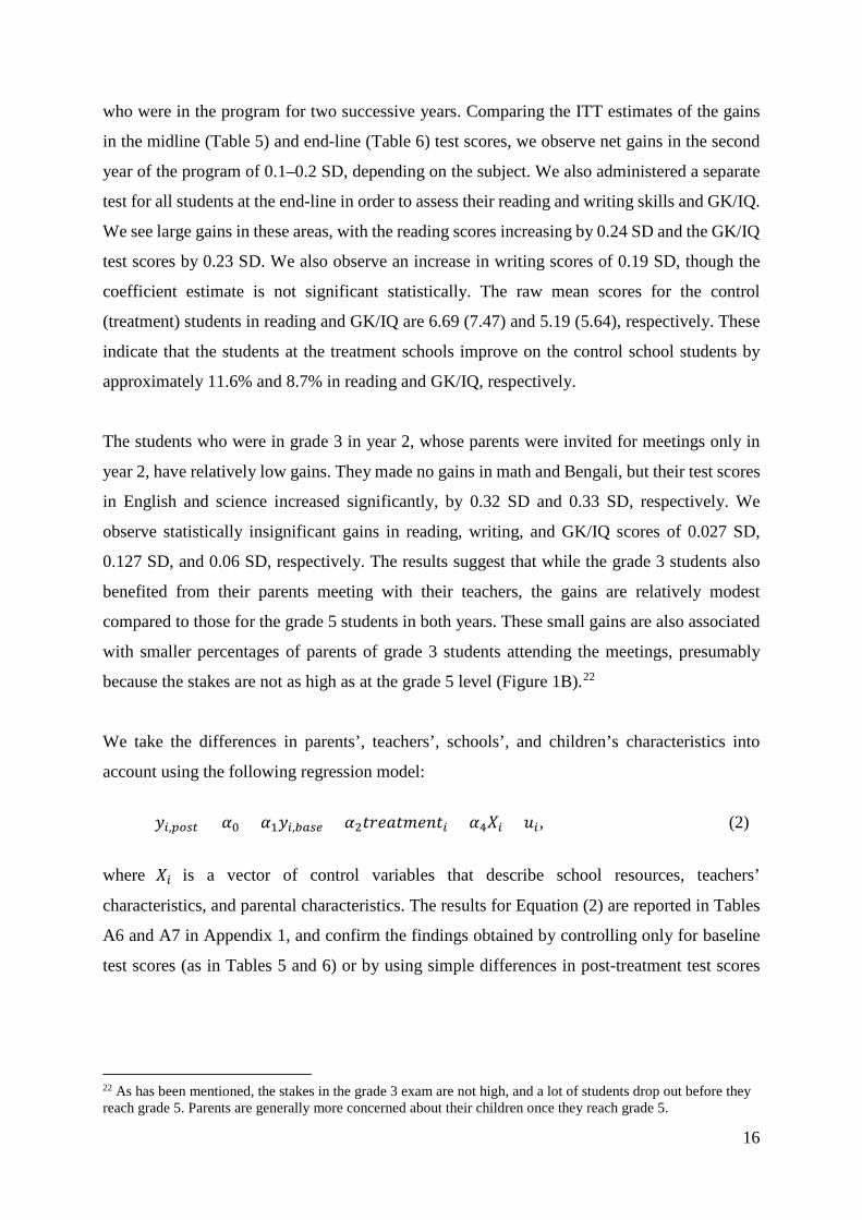
who were in the program for two successive years. Comparing the ITT estimates of the gains

in the midline (Table 5) and end-line (Table 6) test scores, we observe net gains in the second

year of the program of 0.1–0.2 SD, depending on the subject. We also administered a separate

test for all students at the end-line in order to assess their reading and writing skills and GK/IQ.

We see large gains in these areas, with the reading scores increasing by 0.24 SD and the GK/IQ

test scores by 0.23 SD. We also observe an increase in writing scores of 0.19 SD, though the

coefficient estimate is not significant statistically. The raw mean scores for the control

(treatment) students in reading and GK/IQ are 6.69 (7.47) and 5.19 (5.64), respectively. These

indicate that the students at the treatment schools improve on the control school students by

approximately 11.6% and 8.7% in reading and GK/IQ, respectively.

The students who were in grade 3 in year 2, whose parents were invited for meetings only in

year 2, have relatively low gains. They made no gains in math and Bengali, but their test scores

in English and science increased significantly, by 0.32 SD and 0.33 SD, respectively. We

observe statistically insignificant gains in reading, writing, and GK/IQ scores of 0.027 SD,

0.127 SD, and 0.06 SD, respectively. The results suggest that while the grade 3 students also

benefited from their parents meeting with their teachers, the gains are relatively modest

compared to those for the grade 5 students in both years. These small gains are also associated

with smaller percentages of parents of grade 3 students attending the meetings, presumably

because the stakes are not as high as at the grade 5 level (Figure 1B).22

We take the differences in parents’, teachers’, schools’, and children’s characteristics into

account using the following regression model:

𝑦𝑦𝑖𝑖,𝑝𝑝𝑝𝑝𝑝𝑝𝑝𝑝 = 𝛼𝛼0 + 𝛼𝛼1𝑦𝑦𝑖𝑖,𝑏𝑏𝑏𝑏𝑝𝑝𝑏𝑏 + 𝛼𝛼2𝑡𝑡𝑡𝑡𝑡𝑡𝑡𝑡𝑡𝑡𝑡𝑡𝑡𝑡𝑡𝑡𝑡𝑡𝑖𝑖 + 𝛼𝛼4𝑋𝑋𝑖𝑖 + 𝑢𝑢𝑖𝑖, (2)

where 𝑋𝑋𝑖𝑖 is a vector of control variables that describe school resources, teachers’

characteristics, and parental characteristics. The results for Equation (2) are reported in Tables

A6 and A7 in Appendix 1, and confirm the findings obtained by controlling only for baseline

test scores (as in Tables 5 and 6) or by using simple differences in post-treatment test scores

22 As has been mentioned, the stakes in the grade 3 exam are not high, and a lot of students drop out before they reach grade 5. Parents are generally more concerned about their children once they reach grade 5.

17

(Tables A4 and A5).23 Overall, the results remain robust whether or not we control for the

characteristics of households, parents, teachers, and schools.

While the effects of the parent–teacher meetings may initially seem large, the magnitudes are

plausible given that the intervention was carried out in remote rural primary schools in a

developing country. Students from such low socioeconomic backgrounds are more likely to

benefit the most from such interventions. We compare our results with those from several other

successful interventions in developing countries. Andrabi et al. (2017) found that test scores

increased by 0.11 SD as a result of their village-level information campaign intervention in

Pakistan. The Balsakhi program in urban India, which provided low-performing students with

additional teaching hours with a contract teacher (the Balsakhi), increased test scores by an

average of 0.14 SD in its first year (Banerjee et al., 2007). The Extra Teacher Program in Kenya

(Duflo et al., 2011), which also hired contract teachers, resulted in a 0.31 SD gain. The

Computer-Assisted Learning program (Banerjee et al., 2007), which was also conducted in

urban India, increased math scores by 0.36 SD in its first year. However, although these

interventions had positive impacts on the students’ performances, they were costlier and had

generally smaller treatment effects than our intervention.24 A recent study of technology-aided

instruction in India by Muralidharan, Singh and Ganimian (2017) found relatively stronger

effects (0.36 SD in math and 0.22 SD in Hindi) for an intervention that lasted only four and a

half months.

5.2.2 Treatment-On-Treated Effects

When the take-up is low, the TOT effect can be evaluated separately. In the treatment schools,

90% of the students’ parents attended at least one of the five monthly meetings in year 1, while

more than 95% of parents attended two or more meetings in year 2. On the other hand, no

structured monthly parent–teacher meetings like the intervention took place at the control

schools. Thus, there is a powerful first-stage effect of assignment in the treatment school on

parent–teacher meetings. Hence, the TOT effect here is likely to be very close to the ITT effect

presented. In practice, one could estimate the TOT parameter by using the variable “Attend” to

indicate whether or not a parent attended a meeting, with assignment to a treatment or control

23 The sample sizes using parental controls are smaller, as is shown in Tables A6 and A7. We surveyed about 60% of the parents from both the treatment and control schools. 24 It is to be noted that the effect sizes cannot be compared directly because of differences in assessment. Nevertheless, we chose to consider results from some similar studies in order to put things in perspective.

18

school as an instrument, and then running two-stage least squares. In our case, the TOT is the

ITT/take-up rate. With a take-up rate of nearly 90%, the TOT parameter is approximately 1.1

times as high as the ITT estimates presented in Tables 7 and 8.

Next, we examine whether the children of parents who attended more meetings tend to achieve

higher test scores. Table A8 reports the results from a regression of end-line test scores on the

number of meetings, conditioning on parental, teacher, and school characteristics. We run the

regression in Table 7 among only treatment school students. The results indicate that an

additional meeting is associated with a 0.10 SD–0.15 SD increase in test scores, depending on

the students’ subjects and grades. Note though that these results cannot be interpreted as causal

effects, since the decision to participate in a given number of meetings is endogenous.

However, the incremental benefit of an extra meeting with teachers may not be constant. As

parents learn more about their child’s level and progress by attending a few meetings, or perhaps

even only one, the benefit of having more meetings is likely to diminish. On the other hand,

attending more meetings might make parents feel more confident about asking questions or

interacting with teachers. Hence, attending more meetings could enhance the likelihood of

effective interactions and engagements with teachers.

5.3 Distributional Effects

We next check whether the program had different effects depending on students’ abilities

(baseline test scores) before the intervention. We split the students into three groups (as per

Banerjee et al., 2007): top, middle, and bottom thirds by their rankings in the baseline test

distribution,25 and estimated Equation (1) separately for each of the three groups. The results,

without controlling for covariates, are similar, and are not reported here for the sake of brevity.

Table 7 reports the estimated treatment effects for the three groups. It appears that the high

ability students (top 33%) gained the most at the midline tests, and the differences in gains

relative to their counterparts in the middle ability (middle third) and low ability (bottom third)

groups are also statistically significant. In grade 4, after year 1 of the intervention, the high

ability students’ overall test score gains are almost double those of the low ability students (0.49

SD vs. 0.26 SD). The treatment effect is positive and highly significant for students in the top

third (high ability) for all subjects except for science, in the low ability only for math and

25 We used an average over all subjects when ranking students.

19

English, and in the middle ability only for Bengali. The high ability students in grade 5 also

have more than double the gains of other students in CGPA scores. These gains are higher both

separately for all of the individual subjects of the grade 4 students and for the overall GPA of

the grade 5 students. Thus, in the short term, the meetings in year 1 benefited the high ability

students most.

However, at the end of the second year, we see that the effects are quite similar across student

groups, with the lower ability students gaining almost as much as the higher ability students.

The gains in the overall test scores are not statistically different across the three groups of

students in grade 5 (who were also in the program in grade 4), which suggests that the

incremental gains from ongoing parent–teacher meetings are higher among low ability students,

although they might not benefit in the very short term. It is also possible that these parents take

longer to prepare themselves to be able to help their children at home. However, it should be

noted that though the difference in the gains in test scores among these groups of students

diminished over time, we still observed some significant differences across subjects, especially

between the low-ability and high-ability students, in English, science, and Bengali.

Among grade 3 students, some evidence from our findings suggests that the positive gains

accrue more to the lower ability (bottom and middle thirds) of students. We only find

statistically significant gains in English, science, and the overall test scores, with mid- and low-

ability students seeing the highest gains. Low-ability students might be benefiting more from

more frequent interactions with their parents. More meetings between parents and teachers

could lead to more interactions between students and parents. There were more meetings with

teachers in year 2. These frequent meetings might make the parents more comfortable in

interacting with teachers and other parents, thus allowing them to learn more.26 Thus, it is

worthwhile to incentivize or nudge parents to attend meetings, especially the parents of low-

ability children. Indeed, we see that meeting attendance is higher among the parents of lower-

ability students in grade 3 than among their counterparts in grade 5, while the attendance of

parents of high-ability grade 3 students is lower than that of their grade 5 counterparts (Figure

A5). This finding suggests that more frequent meetings could be associated with better

performances among lower-ability children in the classroom.

26 One could also argue that the parent–teacher meetings in year 2 were more organized and systematic because more meetings were held.

20

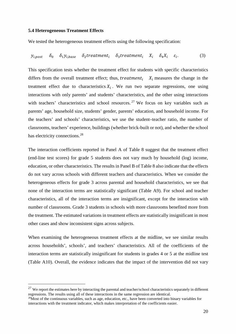
5.4 Heterogeneous Treatment Effects

We tested the heterogeneous treatment effects using the following specification:

𝑦𝑦𝑖𝑖,𝑝𝑝𝑝𝑝𝑝𝑝𝑝𝑝 = 𝛿𝛿0 + 𝛿𝛿1𝑦𝑦𝑖𝑖,𝑏𝑏𝑏𝑏𝑝𝑝𝑏𝑏 + 𝛿𝛿2𝑡𝑡𝑡𝑡𝑡𝑡𝑡𝑡𝑡𝑡𝑡𝑡𝑡𝑡𝑡𝑡𝑡𝑡𝑖𝑖 + 𝛿𝛿3𝑡𝑡𝑡𝑡𝑡𝑡𝑡𝑡𝑡𝑡𝑡𝑡𝑡𝑡𝑡𝑡𝑡𝑡𝑖𝑖 × 𝑋𝑋𝑖𝑖 + 𝛿𝛿4𝑋𝑋𝑖𝑖 + 𝜀𝜀𝑖𝑖. (3)

This specification tests whether the treatment effect for students with specific characteristics

differs from the overall treatment effect; thus, 𝑡𝑡𝑡𝑡𝑡𝑡𝑡𝑡𝑡𝑡𝑡𝑡𝑡𝑡𝑡𝑡𝑡𝑡𝑖𝑖 × 𝑋𝑋𝑖𝑖 measures the change in the

treatment effect due to characteristics 𝑋𝑋𝑖𝑖 . We run two separate regressions, one using

interactions with only parents’ and students’ characteristics, and the other using interactions

with teachers’ characteristics and school resources. 27 We focus on key variables such as

parents’ age, household size, students’ gender, parents’ education, and household income. For

the teachers’ and schools’ characteristics, we use the student–teacher ratio, the number of

classrooms, teachers’ experience, buildings (whether brick-built or not), and whether the school

has electricity connections.28

The interaction coefficients reported in Panel A of Table 8 suggest that the treatment effect

(end-line test scores) for grade 5 students does not vary much by household (log) income,

education, or other characteristics. The results in Panel B of Table 8 also indicate that the effects

do not vary across schools with different teachers and characteristics. When we consider the

heterogeneous effects for grade 3 across parental and household characteristics, we see that

none of the interaction terms are statistically significant (Table A9). For school and teacher

characteristics, all of the interaction terms are insignificant, except for the interaction with

number of classrooms. Grade 3 students in schools with more classrooms benefited more from

the treatment. The estimated variations in treatment effects are statistically insignificant in most

other cases and show inconsistent signs across subjects.

When examining the heterogeneous treatment effects at the midline, we see similar results

across households’, schools’, and teachers’ characteristics. All of the coefficients of the

interaction terms are statistically insignificant for students in grades 4 or 5 at the midline test

(Table A10). Overall, the evidence indicates that the impact of the intervention did not vary

27 We report the estimates here by interacting the parental and teacher/school characteristics separately in different regressions. The results using all of these interactions in the same regression are identical. 28Most of the continuous variables, such as age, education, etc., have been converted into binary variables for interactions with the treatment indicator, which makes interpretation of the coefficients easier.

21

significantly across the characteristics of the participating students’ families, teachers, or

schools.

5.5 Mechanisms

Parent–teacher interactions at these meetings could influence the children’s educational

outcomes in a number of ways. As has been discussed, any parent–teacher meetings would be

likely to affect the behaviors of teachers, parents, and students. For example, Avvisati et al.

(2014) found parent–school meetings to lead to improvements in the behaviors and attitudes of

children, as well as to increased school and home-based activities by parents. Our intervention

entailed both report cards and oral guidelines. Thus, our parent–teacher meetings involved a

behavioral or instructional component (e.g., information on how to best help children at home,

which could change parental behavior), an informational component (parents learn about their

children’s performance), and an accountability component for both parents and teachers, as they

met and could hold each other accountable for a student’s performance. This is a reasonable

way to structure an intervention, since no meeting between parents and teachers is complete

without these three elements. It is difficult to isolate the effects of each aspect of the meetings

or the relative contribution of each. Below, we provide some evidence regarding the channels

through which test scores and other outcomes are most likely to be impacted.

5.5.1 Do Teachers’ Pedagogy and Efforts Respond to Intervention?

The evidence in the previous section shows clearly that the regular parent–teacher monthly

meetings led to significant improvements in student achievements on test scores in math,

English, and science. It also enhanced the students’ general knowledge and reading and writing

skills. However, these improvements could be due to increases in teacher efforts as a result of

the meetings. The teachers might put in more effort in order to either improve their

accountability or meet new demands from parents following the meetings. Since teachers in the

treatment and control schools were paid equally, we do not expect any differential change in

behavior due to such payments. We also showed (Table 3) that the teachers in treated and

untreated schools have similar characteristics. In addition, the treatment and control schools

have similar infrastructure and facilities. Thus, the gains in the students’ academic

achievements are not due to differences in teacher and school characteristics. It should be noted

that the intervention did not ask the teachers to change anything that they usually did at school

for teaching their students (e.g., an increased monitoring of their classroom presence or the

performances of the children, changing their teaching styles, etc.). There was also no change in

22

the provision of school resources, curriculum, or school inputs (e.g., textbooks). However, we

cannot rule out the possibility that the intervention had some effects on teachers’ effort. For

example, teachers might have increased their efforts to teach the students or made the school

environment more friendly or welcoming so that the children were more likely to come to

school. We investigate a few possible channels below.

First, we examine the absence of teachers from school. Previous studies have found high rates

of teacher absenteeism in many developing countries, including Bangladesh (Chaudhury et al.,

2006).29 In an attempt to understand the effects on teacher absenteeism, field staff members

made random visits to all schools on days other than those of the meetings in order to check for

teachers’ absences. If a teacher could not be found in the school compound for any reason

during the random unannounced spot visit, he or she was considered absent on that day. We see

some evidence that teacher absenteeism was somewhat lower in the treatment schools, but the

difference is not statistically significant (Table A11). Each school has an average of five

teachers, and we find that, on average, more than two teachers were absent in total during eight

unannounced visits to a given school. Thus, a random visit in a given month found an average

of approximately 0.3 of five teachers absent, resulting in an absence rate of about 6%. Overall,

the teachers’ absence rates in both the treatment and control schools were lower than has been

suggested by some studies on teacher absences in developing countries (see for example

Chaudhury et al., 2006). However, this difference could be due to the frequent visits to these

schools (both treatment and control) at other times by field staff members (to conduct meetings

at the treatment schools and to administer baseline and follow-up exams, collect information

from report cards, and survey both students and teachers at both the treatment and control

schools).30 Thus, the lower absence rate in this study may not be directly comparable with that

of Chaudhury et al. (2006). Overall, the point estimates suggest somewhat lower absence rates

of teachers in the treatment schools, though the differences are not significant. The mean teacher

absence rates were low (6%), and the difference in the numbers of days that teachers were

absent between the treatment and control schools is unlikely to be a significant determinant of

the improvement in students’ test scores.31

29 Chaudhury et al. (2006) found an absence rate of 23.5% among teachers in Bangladeshi primary schools in one of the two random visits to schools, with higher levels of absenteeism in rural areas. 30 These schools also received letters from local education officers offering to help in conducting the research, especially in running the surveys, meetings (treatment schools only), and students’ tests. 31 In a separate regression, we also examined the correlates of teacher absenteeism, but we did not find any significant predictor of teachers’ characteristics for absenteeism, and the interaction terms of the treatment dummy

23

However, teacher efforts could change in other ways, even if the impact on their absences is

not significant. It is possible that teachers changed their pedagogical practices. In order to

understand this, we asked the teachers at the end of year 2 of the intervention about their

teaching practices in the classroom. About 25% of the teachers in the treatment schools

mentioned that they generally relied only on textbooks, as opposed to 51% in the control schools

(Table A12). Nearly 70% of the teachers in the treatment schools reported using real-life

examples such as relating materials to the outside world, using maps, pictures, diagrams, and

charts. On the other hand, only 48% of teachers in the control schools used such materials as

their main teaching aids. Thus, we observed treatment school teachers making greater efforts

to teach students, in terms of using visual aids and multiple representations of concepts. In order

to understand how much of the gain in students’ test scores is due to differences in the

instruction methods used by teachers in the treatment schools, we control these variables

(dummy variables of whether or not a textbook is used as the main teaching tool and whether

visual aids are used for teaching) in a regression analysis of test scores. The treatment effects

do not change significantly, and the statistical significance remains unchanged.

It is also possible that the teachers paid more attention to their students’ grades because they

were having meetings with the parents. We wanted to evaluate and observe the teachers’ efforts,

teaching practices and instruction methods in the classroom directly by observing them in the

classroom through independent evaluators. However, that was not possible due to

discouragement from teachers and local educational administrations. There were also no

independent teaching evaluations conducted by schools or teachers. We were told that such

observations or monitoring of teachers might have unintended consequences, as the teachers

might feel threatened, 32 and therefore would not cooperate in the implementation of the

program.

The intervention might have also changed the behavior of teachers (and parents) such that they

were more concerned about the students’ attendance at school. We checked student attendance

data from class rosters in both years. On average, students were absent on 2.1 days in treatment

schools and 1.7 days in control schools (Table A13) during the first month after the intervention

and the teachers’ characteristics are all statistically insignificant. We also added the number of days that teachers were absent to regressions on test scores, but the treatment coefficients remained unchanged. 32 For example, the teachers were concerned about us reporting to the local educational administration about their teaching practices, even though we gave full assurance that any information would be kept confidential and would be used only for research purposes.

24

(June 2011). In year 1 (2011), the absences declined more in treatment schools than in control

schools, suggesting an improvement in children’s attendance at the treatment schools. In year

2 (2012), though, we did not see any significant difference in students’ attendance. The

students’ presence varied somewhat across months, with the control schools having slightly

higher absence rates than the treatment schools.

Overall, we see changes in teachers’ efforts in terms of altering their instruction methods and

being more present at school, along with the more frequent presence of students at school. These

changes following intervention are not unexpected, given regular parent–teacher interactions

through organized meetings. The next sub-section examines changes in parental engagement at

home.

5.5.2 How Much Did Parental Involvement Increase?

Regular information on children’s school performances may encourage an increase in parental

involvement. The intervention might have motivated parents to provide a supportive home-

learning environment, including talking with the child about their learning and providing

resources that foster continuous home-to-school communication. Furthermore, we also

examined whether any changes in parental engagement persisted after the intervention finished.

Table 9 (Panel A) reports parents’ evaluations of their children one year after the end of the

intervention. We conducted a follow-up survey at the household level in early 2014, more than

a year after the intervention ended, which allowed us to also examine whether the treatment

effect was sustained after the end of the intervention, making long-lasting differences to

children’s future educational aspirations. 33 We randomly surveyed about 60% of the

households in both the treatment and control groups.34 The test scores of the children in the

households that were surveyed do not differ from those in the households that were not.

The results presented in Panel A of Table 9 indicate that there was still a greater parental

involvement one year after the intervention ended: the fathers, mothers, and older siblings of

the children in the treatment schools were more likely to help them with their study. The parents

of the children in the treatment schools reported that their children had more private tutors (40%

33 We avoided asking the parents these questions during the intervention in order to avoid the potential Hawthorne effect. While this is less of a concern after over a year, we cannot rule out changes in the parents’ behaviors completely, as they were invited to the meetings. 34 We attempted to visit either odd or even-numbered students by their class roll numbers, which are based on their classroom rankings.

25

in treatment schools compared to only 18% in control schools) and were less likely to fail to

progress to the next grade. These children also spent less time at home doing household chores.

The parents in the treatment schools also placed less importance on private tutoring for their

children’s educational improvement (62% in treatment versus 72% in control), and more

emphasis on helping their children at home. There is no evidence that parents were substituting

their own time for private tuition. Instead, we observed an increased involvement of families in

their children’s education. The teachers also did not encourage parents to seek additional

tutoring; indeed, they were specifically asked not to give any such instruction. However, it

could be that the information provided in the meetings (e.g., the report cards) helped to identify

specific deficiencies that the parents felt tutoring could address. There may also have been some

parents who were unable to help their children at home, and these parents might have sent their

children to tutors as a result of the meetings. The household survey asked parents in the

treatment group for their opinion of the parent–teacher meetings in this intervention. Most of

the parents in the treatment schools thought that the parent–teacher meetings contributed to the

students’ learning, and more than 90% believed that they should continue (Table A14).

5.5.3 Student Attitudes and Behaviors

The parental evaluations are consistent with the students’ self-reported evaluations, conducted

immediately after the program ended in late 2012. The results are presented in Panel B of Table

9. Children in the treatment schools were more likely to have a proper breakfast before going

to school (53%) than those in the control schools (48%). The students in the treatment group

were also more ambitious: 28% wanted to be either a doctor or an engineer, while only 20% of

children in the control schools expressed the same ambition. The students in the treatment

schools also had more positive behaviors toward their classmates and were more likely to do

their homework regularly. They spent about 1.1 more hours per week studying at home, which

is more than a quarter of an hour extra per day. Finally, the treatment group students felt more

confident before exams; 70% of students in the treatment schools and 59% in the control

schools reported feeling confident in sitting for the exam.

5.5.4 Teachers’ Evaluations about Students

We also find that students’ evaluations are consistent with those of their teachers. The class

teachers in both the treatment and control schools reported on the behavior and performance of

each student. They were asked to report several items about each student at the end of the

intervention in 2012, including their attendance, class performance and homework, and an

26

overall assessment of the student’s character, discipline, and honesty. On the whole, the

teachers reported 92% of children in the treatment schools and 88.5% in the control schools to

have good attendances, while 85% of children in the treatment schools and 79% in the control

schools were reported to have good performances (Panel C, Table 9). The students in the

treatment schools also turned in their homework more regularly: 83% of students in the

treatment schools and 77% in the control schools, as reported by teachers. When asked to assess

each child’s overall behavior, discipline, and honesty, the teachers in the treatment schools

reported that 77% of children behaved very well, while the number in the control schools was

73%. Overall, the teachers’ assessments suggest that the students who were targeted by the

program directly developed more positive behaviors and attitudes at school. These results

indicate that schools can improve teachers’ perceptions and students’ cognitive and non-

cognitive behaviors through interactions with parents, engaging them directly in their children’s

education.

5.6 Spillover Effects

We also examine the spillover effects among students who were in grade 4 in year 2 and whose

parents were not invited to any meetings. These students were in grade 3 in year 1 and were not

part of the intervention in any year. However, the intervention might have had effects on the

untreated students in the treatment schools through parental social networks, since they meet

frequently in their own villages. Similarly, teachers teach in multiple grades, and if a teacher

changed her teaching style in a treated grade, she may have done so in a non-treated grade as

well, or she may have discussed this change with other teachers in the school.

The results in Table 10 suggest that there were some positive spillover effects. The ITT

estimates for the year 2 grade 4 students in the treatment and control schools suggest that the

English test scores of students in the treatment schools improved by 0.25 SD. We did not see

any other significant differences, except for a 0.35 SD increase in writing scores. The effects

on the other subjects were positive but not statistically significant. The overall mean test scores

were 0.11 SD higher, but the effect is not statistically significant. This represents a spillover

effect size of about 25% of the ITT effects.

5.7 Cost-Effectiveness of the Intervention

The intervention is remarkably low cost. We paid each teacher only $25 per academic year to

conduct the meetings, meaning that the total added cost for teachers to run the program in a

school was $125 per academic year. Even when we include the costs of hiring field staff

27

members and organizing meetings with parents, the cost for each school is still less than $300

per academic year. This amounts to about $1.25 per student per academic year for the teacher

costs,35 or $3 for the full program costs (including the costs of preparing report cards and hiring

field staff to facilitate the meetings).36 If we consider the estimate in Table 6, the meetings

raised the students’ overall test scores by 0.38 SD by the end of the program’s second year.

Thus, the cost per average 0.1 SD increase in test scores per student is $0.66 or $1.58 for the

full program over 2 years.37

Parent–teacher meetings are routine in schools in many countries, and the Bangladeshi

government does officially mandate that school teachers meet regularly with parents. In

practice, though, no such meetings happen in public schools, with a few exceptions in select,

urban public schools. These meetings could be almost free of cost if the government were to

enforce the mandate for them. Thus, this program could be less costly to scale up than other

similar programs that have been evaluated. However, note that it is difficult to compare the

cost-effectiveness of different educational interventions implemented across a range of

countries due to differences in context, reporting about estimated effect sizes, and outcomes of

interest. There are also differences in testing instruments, costs and prices, and target

populations. On the surface, however, it seems that our intervention is more cost-effective than

any of those studied by either Kremer et al. (2013) or Glewwe and Muralidharan (2016). For

example, Kremer et al. (2013) studied 15 interventions, with (statistically significant) effect

sizes ranging from 0.14 SD to 0.6 SD for each $100 spent in those studies. 38 If we follow the

same approach as Kremer et al. (2013), our results indicate that we could obtain more than a

few fold increase in test scores for each $100 spent on our program (including administrative

and other expenses).39

6. Conclusion

The purpose of this study was to examine the effectiveness of a low-cost strategy for improving

the behaviors of both education providers (teachers) and recipients (pupils) by holding regular

35 On average, there are about 50 students in each grade. The total costs include costs for both grades (grades 4 and 5 in year 1, and grades 5 and 3 in year 2), with about 100 students in total each year. 36 These estimates do not include the costs associated with administering the tests for the project in the schools because exams are an integral, routinely-conducted part of education, and there will be no need for independent exams once the system of parent–teacher meetings is in place and enforced. 37 Ignoring the opportunity cost of parents’ time in attending the meetings. 38 The least expensive program evaluated and considered in these studies was the Balsakhi Program in India, where the corresponding cost was $0.67 per 0.1 SD increase in test scores. 39 This is calculated as the effect size reported in Table 6 multiplied by the number of children under consideration, divided by the total cost of the program in hundreds of dollars.

28

meetings in order to inform parents about the educational progress of their primary school

children. A report card was prepared for each child for each meeting as part of the provision of

information about a child’s academic progress at school, and the parents also engaged in one-

on-one consultations with teachers to receive feedback about the performances of their children.

Engaging parents in their children’s education, both at home and at school, is a potentially

important way of supporting better learning outcomes. This paper presents strong evidence that

parental involvement in school activities can have a significant positive effect on the students’

learning, even in low-income countries. Overall, the program increased the students’ test scores

by 0.26 SD by the end of year 1 and 0.38 SD by the end of year 2. The students’ reading and

writing skills also improved, as along with their general knowledge. We also found the

intervention to have effects on the teachers’ efforts and pedagogical practices. This paper shows

that the full effects of such programs take some time to become visible. In the short term, higher-

ability students (those with baseline test scores in the top third) benefited more from the

program; but over time, as the meetings progressed, the low-ability students gradually began to

benefit too. The treatment effect is stable and robust and is observed regardless of either the

education level or experience of the teachers or the socioeconomic backgrounds of the students.

The results show that the intervention induced parents and other household members to spend

more time at home helping the children study or do homework. The intervention also helped to

improve the attitudes, behavior, and confidence of the children.

Our main conclusion, namely that increased parent–teacher meetings that also provide

information about a child’s academic progress through a report card can be a cost-effective tool

for improving students’ outcomes, has important policy implications. Such programs are low-

cost and easy to implement, even in disadvantaged communities where parents have low levels

of literacy. In the context of developing countries, there is not enough evidence of what a simple

one-on-one parent–teacher scheduled meeting can do to improve students’ educational

achievements. Our results demonstrate that even parents from disadvantaged backgrounds in

developing countries can make significant contributions to their children’s school performances

if they are provided with adequate information and encouraged to become involved.

29

References

Afridi, F. (2010) Child welfare programs and child nutrition: evidence from a mandated school meal program. Journal of Development Economics, 92(2), 152–165.

Andrabi, T., Das, J., & Khwaja, A. I. (2017). Report cards: The impact of providing school and child test scores on educational markets. American Economic Review, 107(6), 1535–1563.

Avvisati, F., Gurgand, M., Guyon, N., & Maurin, E. (2014). Getting parents involved: A field experiment in deprived schools. Review of Economic Studies, 81(1), 57–83.

BANBEIS (2013). Bangladesh education statistics. Dhaka: Bangladesh Bureau of Educational Information and Statistics.

Banerjee, A., Banerji, R., Duflo, E., Glennerster, R., & Khemani, S. (2010). Pitfalls of participatory programs: Evidence from a randomized evaluation in education in India. American Economic Journal: Economic Policy, 2(1), 1–30.

Banerjee, A., Cole, S., Duflo, E., & Linden, L. (2007). Remedying education: Evidence from two randomized experiments in India. Quarterly Journal of Economics, 122(3), 1235–1264.

Banerjee, A., & Duflo, E. (2006). Addressing absence. Journal of Economic Perspectives, 20(1), 117–132.

Banerji, R., Berry, J., & Shotland, M. (2017). The impact of mother literacy and participation programs: Evidence from a randomized evaluation in India. American Economic Journal: Applied Economics, 9(4), 303-337.

Barrera-Osorio, F., Bertrand, M., Linden, L. L., & Perez-Calle, F. (2011). Improving the design of conditional transfer programs: Evidence from a randomized education experiment in Colombia. American Economic Journal: Applied Economics, 3, 167–195.

Bergman, P. (2016). Parent-child information frictions and human capital investment: Evidence from a field experiment investment. Working paper.

Chaudhury, N., Hammer, J., Kremer, M., Muralidharan, K., & Rogers, F. H. (2006). Missing in action: Teacher and health worker absence in developing countries. Journal of Economic Perspectives, 20(1), 91–116.

Das, J., Dercon, S., Habyarimana, J., Krishnan, P., Muralidharan, K., & Sundararaman, V. (2013). School inputs, household substitution, and test scores. American Economic Journal: Applied Economics, 5(2), 29–57.

Dizon-Ross, R. (2017). Parents’ beliefs about their children’s academic ability: implications for educational investment. Working Paper, University of Chicago.

Duflo, E., Dupas, P., & Kremer, M. (2011). Peer effects, teacher incentives, and the impact of tracking: Evidence from a randomized evaluation in Kenya. American Economic Review, 101(5), 1739–1774.

Gelber, A. & Isen, A. (2013). Children's schooling and parents' investment in children: Evidence from the head start impact study. Journal of Public Economics, 101, 25–38.

Glewwe, P., Kremer, M., & Moulin, S. (2009). Many children left behind? Textbooks and test scores in Kenya. American Economic Journal: Applied Economics, 1(1), 112–135.

Glewwe, P., Kremer, M., Moulin, S., & Zitzewitz, E. (2004). Retrospective vs. prospective analyses of school inputs: The case of flip charts in Kenya. Journal of Development Economics, 74(1), 251–268.

Glewwe, P. & Muralidharan, K. (2016). Improving education outcomes in developing countries – evidence, knowledge gaps, and policy implications. In E. Hanushek & L. Woessman (eds.), Handbook of the Economics of Education, Volume 5.

30

Hahn, Y., Islam, A., Nuzhat, K., Yang, H-S., & Smyth, R. (2018). Education, marriage and fertility: Long-term evidence from a female stipend program in Bangladesh. Economic Development and Cultural Change, 66(2), 383-415.

Hahn, Y., Islam, A., Mahmooei, B., Patacchini, E., & Zenou, Y. (2016). Does friendships matter in female education: the case of Bangladesh. CEPR Discussion Paper No. 11615.

Hastings, J. S., & Weinstein, J. M. (2008). Information, school choice, and academic achievement: Evidence from two experiments. Quarterly Journal of Economics, 123(4), 1373–1414.

Holbrook, J. (2005). Report on organizing the ROSE survey in Bangladesh. Faculty of Educational Sciences, University of Oslo.

Houtenville, A. J., & Conway, K. S. (2008). Parental effort, school resources, and student achievement. Journal of Human Resources, 43(2), 437–453.

Kremer, M., Brannen, C. & Glennerster, R. (2013). The challenge of education and learning in the developing world. Science, 340(6130), 297–300.

Lee, D. S. (2009). Training, wages, and sample selection: Estimating sharp bounds on treatment effects. Review of Economic Studies, 76(3), 1071–1102.

Lieberman, E., Posner, D. & Tsai, L. (2014). Does information lead to more active citizenship? Evidence from an education intervention in rural Kenya. World Development, 60, 69–83.

Mbiti, I. (2016). The need for accountability in education in developing countries. Journal of Economic Perspectives, 30(3), 109–32.

Muralidharan, K. Singh, A., & Ganimian, A. (2017) Disrupting education? Experimental evidence on technology-aided instruction in India. NBER Working Paper No. 22923

Muralidharan, K. & Prakash, N. (2017) Cycling to school: increasing secondary school enrolment for girls in India. American Economic Journal: Applied Economics, 9(3), 321–350.

Muralidharan, K. & Sundararaman, V. (2013). Contract teachers: Experimental evidence from India. NBER Working Papers 19440.

Nguyen, T. (2008). Information, role models and perceived returns to education: Experimental evidence from Madagascar. Working paper.

Pop-Eleches, C., & Urquiola, M. (2013). Going to a better school: effects and behavioral responses. American Economic Review, 103(4), 1289–1324.

Tapan, M. (2010). Science education in Bangladesh. In Y.-J. Lee (Ed.), World of science education: science education research in Asia. Rotterdam, Boston: Sense Publishers.

UNESCO (2010). World data on education: Bangladesh. UNESCO-International Bureau of Education, VII Ed. 2010/11.

31

Table 1: Parent–teacher Meetings by Year and Grade

Program in Year 1 (in 2011)

Program in Year 2 (in 2012)

Follow-up (in 2014)

Grade 3 (Year 2) ✓ ✓

Grade 4 (Year 1) ✓ ✓ ✓

Grade 5 (Year 1) ✓ ✓

Notes: The cohort that was in grade 4 in 2011 (year 1) was in grade 5 in 2012 (year 2). Hence, the program was available for both years for this cohort. For the students who were in grade 5 in year 1, the program was available only in that year. Grade 3 students (who had been in grade 2 in year 1) were added as part of the intervention in year 2.

Table 2: Test for Differences in the Mean Baseline Test Scores Math English Science Bengali GK/IQ

Grade 4 Year 1 (Baseline)

Difference 0.0587 –0.0391 –0.0282 0.0228 –0.0179

S.E (0.0411) (0.0416) (0.0382) (0.0428) (0.0362) N T = 1244 C = 1059

Grade 5 Difference –0.0461 –0.0683 0.0159 –0.0541 0.0021

S.E (0.0404) (0.0430) (0.0444) (0.0432) (0.0419) N T = 1046 C = 717

Grade 3 Year 2 (baseline) Difference –0.0582 –0.0046 0.0103 0.0180 0.0602

S.E (0.0391) (0.0384) (0.0209) (0.0203) (0.0399) N T = 1222 C = 1186

Notes: This table gives the simple mean differences in normalized pre-intervention test scores between the treatment and control school students, conducted at the beginning of the academic year. The control group mean and standard deviation are 0 and 1, respectively. Standard errors (S.E) of the differences are presented in the second row in brackets. None of the differences are statistically significant.

32

Table 3: School and Teacher Characteristics Treatment Control Diff S.E t-stat (T – C) I II III IV V Number of teachers 5.2 4.8 0.45 0.33 1.35

Number of female teachers 2.8 2.6 0.24 0.35 0.69

Number of students in grades 4 and 5 60.8 61.3 –0.55 6.53 0.08

Number of classrooms 4.22 4.35 –0.13 0.32 0.39

Student–classroom ratio 50.6 53.3 –2.70 6.21 0.43

Years in a teaching job (experience) 10.9 8.8 2.18 0.96 2.28

Amount of professional training 1.9 1.8 0.11 0.12 0.30

Years of education 18.7 20.2 –1.43 0.23 6.33

Distance travelled from home to school (km) 5.0 4.2 0.93 0.81 0.95

Monitoring of schools by TEO* (satisfactory) 0.68 0.64 0.04 0.05 0.79

Electricity connection in school area 0.68 0.58 0.10 0.11 0.82

Drinking water facility 0.13 0.22 –0.09 0.09 1.12 Notes: This table gives the average characteristics of the treatment and control schools, and the differences before the intervention begins in year 1 (2011). Standard errors (S.E.) and (absolute values of the) t-statistics of the differences are presented in columns (IV) and (V), respectively. Statistically significant differences are given in bold. *TEO = Thana (sub-district) Education Officer

Table 4: Correlates of Parental Presence at Meetings (Poisson Regression Model) Dependent variable: (1) (2) (3) (4) Number of meetings attended Year 1 Year 2 Age of the household head –0.00148 –0.00172 –0.00449** –0.00235 (0.00275) (0.00271) (0.00179) (0.00178) Household size 0.00987 0.00661 0.00949 0.00300 (0.0148) (0.0130) (0.00837) (0.00855) Head above primary education –0.0499 –0.0307 0.0152 –0.0186 (0.0430) (0.0351) (0.0230) (0.0208) Mother above primary education 0.0219 0.0160 0.0428 0.0401 (0.0429) (0.0370) (0.0384) (0.0380) (Log) household income –0.136 –0.0993 0.0274 0.0323 (0.0734) (0.0659) (0.0329) (0.0359) Gender of household head 0.0512 0.0534 0.133* 0.0998 (0.0710) (0.0857) (0.0743) (0.0841) Gender of student (female = 1) 0.00709 0.0107 –0.0139 –0.0195 (0.0268) (0.0218) (0.0143) (0.0156) Grade dummy (grade five = 1) –0.168 –0.140 0.0482 –0.00900 (0.0908) (0.0896) (0.0324) (0.0388) baseline Bengali 0.00790 0.00390 (0.0301) (0.00933) baseline English –0.0228 –0.0174** (0.0162) (0.00799) baseline mathematics –0.00649 0.000594 (0.0179) (0.00611) baseline science –0.0156 0.0118 (0.0286) (0.00716) baseline GK/IQ 0.0528* 0.000883 (0.0245) (0.0106) Observations 2232 2016 1728 1376

Notes: The last column is based on students from grade 5, as baseline marks for grade 3 students are missing. The sample for year 1 includes the students in grades 4 and 5 (and their parents, in this table) in that year, while the sample for year 2 consists of those in grades 5 and 3 in year 2. The overall sample size is smaller than the total number of students, as the parental survey was conducted on a subset of samples selected randomly. Standard errors are clustered at the school level and reported in parentheses. * p < 0.05, ** p < 0.01, *** p < 0.001.

33

Table 5: ITT Estimates of Test Scores: Midline Results, Year 1 (2011) (1) (2) (3) (4) (5) (6) Grade 4 Grade 5 Math English Science Bengali ALL CGPA Treatment effect 0.224* 0.362** 0.139 0.306*** 0.260** 0.200** (0.118) (0.138) (0.115) (0.112) (0.115) (0.0966) Baseline test score 0.376*** 0.370*** 0.396*** 0.0986** 0.553*** 0.0787 (0.0461) (0.0558) (0.0475) (0.0473) (0.0534) (0.0565) Observations 2197 2203 2202 2204 2204 1768 Adjusted R2 0.149 0.145 0.120 0.031 0.195 0.014 Male (N = 1072) Treatment effect 0.237* 0.398*** 0.151 0.320** 0.259** 0.348*** (0.128) (0.132) (0.120) (0.123) (0.118) (0.102) Female (N = 1025) Treatment effect 0.209* 0.319* 0.123 0.283** 0.254** 0.209* (0.123) (0.162) (0.129) (0.120) (0.124) (0.123)

Notes: This table gives the regression-adjusted treatment effects, conditioning on the baseline test scores (using Equation (1)). The midline tests were conducted after year 1 of the intervention. ‘ALL’ represents the average of the test scores for all subjects (math, English, science, and Bengali). The test scores are normalized, with the baseline mean and standard deviation of the control group being 0 and 1, respectively. Standard errors are clustered at the school level and reported in parentheses. * p < 0.05, ** p < 0.01, *** p < 0.001.

34

Table 6: ITT Effects on Test Scores: End-line Results, Year 2 (2012) (1) (2) (3) (4) (5) (6) (7) (8) ALL Grade 5 (N = 1870) Math English Science Bengali ALL GK/IQ Reading Writing Treatment effect 0.420*** 0.413*** 0.339*** 0.309*** 0.377*** 0.235* 0.244* 0.190 (0.129) (0.126) (0.106) (0.100) (0.0990) (0.128) (0.148) (0.146) Baseline test score 0.210*** 0.171*** 0.219*** 0.167*** 0.281*** 0.412*** 0.219*** 0.258*** (0.0552) (0.0579) (0.0386) (0.0406) (0.0616) (0.0844) (0.0605) (0.0971) Adjusted R2 0.100 0.067 0.086 0.070 0.135 0.120 0.041 0.042 Male (N = 950) Treatment effect 0.370** 0.424*** 0.324*** 0.374*** 0.377*** 0.268** 0.184 0.143 (0.142) (0.140) (0.121) (0.114) (0.108) (0.127) (0.153) (0.138) Female (N = 920) Treatment effect 0.469*** 0.401*** 0.340*** 0.245** 0.371*** 0.203 0.304* 0.242 (0.136) (0.129) (0.112) (0.106) (0.103) (0.153) (0.161) (0.179) ALL Grade 3 (N = 2253) Treatment effect –0.0873 0.317*** 0.332*** –0.00594 0.141 0.00906 0.0529 0.127 (0.0787) (0.0907) (0.107) (0.107) (0.0860) (0.0937) (0.126) (0.149) Baseline test score 0.304*** 0.314*** 0.318*** 0.339*** 0.489*** 0.358*** 0.221*** 0.219*** (0.0334) (0.0367) (0.0391) (0.0381) (0.0482) (0.0402) (0.0543) (0.0657) Adjusted R2 0.091 0.101 0.125 0.120 0.179 0.080 0.029 0.027 Male (N = 1127) Treatment effect –0.0796 0.266*** 0.331*** –0.0368 0.125 0.0427 0.00860 0.203 (0.0871) (0.0928) (0.106) (0.102) (0.0828) (0.105) (0.135) (0.137) Female (N = 1126) Treatment effect –0.0959 0.367*** 0.331*** 0.0247 0.156 –0.0245 0.0969 0.0512 (0.0929) (0.110) (0.123) (0.123) (0.103) (0.112) (0.136) (0.177)

Notes: This table gives the regression-adjusted treatment effects, conditioning on the baseline test scores (using Equation (1)). The end-line tests were conducted after year 2 of the intervention. ‘ALL’ represents the average of the test scores for all subjects (math, English, science, and Bengali). The sample sizes differ slightly, as some students’ test scores were missing or not reported in one or more subjects. The test scores are normalized, so that the baseline mean and standard deviation of the control group are 0 and 1, respectively. For GK/IQ, reading and writing, the test scores are normalized at the end-line, with the control mean and standard deviation being 0 and 1, respectively. Standard errors are clustered at the school level and reported in parentheses. * p < 0.05, ** p < 0.01, *** p < 0.001.

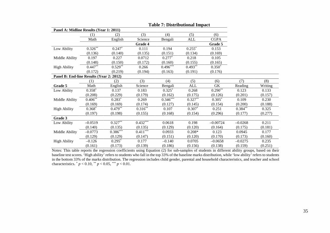
35

Table 7: Distributional Impact Panel A: Midline Results (Year 1: 2011) (1) (2) (3) (4) (5) (6) Math English Science Bengali ALL CGPA Grade 4 Grade 5 Low Ability 0.326** 0.247* 0.111 0.194 0.255* 0.153 (0.136) (0.140) (0.135) (0.151) (0.134) (0.169) Middle Ability 0.197 0.227 0.0712 0.277* 0.218 0.105 (0.148) (0.150) (0.172) (0.160) (0.155) (0.165) High Ability 0.447** 0.529** 0.266 0.496*** 0.493** 0.350* (0.172) (0.219) (0.194) (0.163) (0.191) (0.176) Panel B: End-line Results (Year 2: 2012) (1) (2) (3) (4) (5) (6) (7) (8) Grade 5 Math English Science Bengali ALL GK Reading Writing Low Ability 0.358* 0.137 0.183 0.325* 0.268 0.290** 0.123 0.133 (0.208) (0.229) (0.179) (0.162) (0.175) (0.126) (0.201) (0.157) Middle Ability 0.406** 0.283* 0.269 0.346*** 0.327** 0.305* 0.109 0.230 (0.169) (0.169) (0.174) (0.127) (0.145) (0.154) (0.200) (0.188) High Ability 0.368* 0.479** 0.316** 0.107 0.307* 0.251 0.384** 0.325 (0.197) (0.198) (0.155) (0.168) (0.154) (0.296) (0.177) (0.277) Grade 3 Low Ability –0.0519 0.327** 0.432*** 0.0618 0.198 –0.00724 –0.0268 0.211 (0.140) (0.135) (0.135) (0.129) (0.120) (0.164) (0.175) (0.181) Middle Ability –0.0773 0.386*** 0.411*** 0.0933 0.208* 0.123 0.0945 0.177 (0.129) (0.129) (0.147) (0.151) (0.120) (0.170) (0.173) (0.160) High Ability –0.126 0.295* 0.177 –0.140 0.0705 –0.0658 –0.0275 0.235 (0.161) (0.173) (0.139) (0.186) (0.156) (0.138) (0.159) (0.251)

Notes: This table reports the regression coefficients using Equation (2) for sub-samples of students in different ability groups, based on their baseline test scores. ‘High ability’ refers to students who fall in the top 33% of the baseline marks distribution, while ‘low ability’ refers to students in the bottom 33% of the marks distribution. The regression includes child gender, parental and household characteristics, and teacher and school characteristics. * p < 0.10, ** p < 0.05, *** p < 0.01.

36

Table 8: Heterogeneous effects: Grade 5 (end-line, year 2)

(1) (2) (3) (4) (5) (6) (7) (8) Math English Science Bengali All GK Reading Writing Panel A: Interactions with household characteristics Treatment school*covariate Age of head (above median) 0.333*** 0.132 0.162 0.0157 0.146 0.430*** –0.0729 0.140 (0.125) (0.134) (0.132) (0.112) (0.111) (0.152) (0.145) (0.180) Household size (above median) –0.146 –0.0287 –0.137 0.0763 –0.0373 –0.103 0.171 –0.0224 (0.157) (0.171) (0.139) (0.145) (0.127) (0.155) (0.216) (0.183) Student gender (female =1) 0.0192 0.0826 0.0678 –0.159 0.0142 –0.145 0.210 0.0907 (0.143) (0.121) (0.0962) (0.101) (0.0954) (0.118) (0.127) (0.164) Both parents primary educated 0.171 0.0337 0.0672 0.156 0.0776 0.364*** 0.132 0.0987 (0.153) (0.149) (0.129) (0.117) (0.118) (0.137) (0.162) (0.169) Income above log median –0.220* –0.200 –0.138 –0.157 –0.173 –0.154 0.0121 –0.339* (0.129) (0.134) (0.126) (0.102) (0.107) (0.130) (0.152) (0.171) Panel B: Interactions with school and teacher characteristics Treatment school*covariate Student–teacher ratio –0.0126 –0.0148 –0.00320 –0.00733 –0.0105 0.00326 0.00636 0.00475 (0.0102) (0.0142) (0.00826) (0.00726) (0.00888) (0.00905) (0.0135) (0.0113) Years of teaching experience 0.0128 0.00972 0.0153 0.00250 0.0104 0.0107 0.00617 0.0270 (0.0149) (0.0131) (0.0109) (0.0138) (0.0116) (0.0158) (0.0167) (0.0179) Number of classrooms 0.121 0.0353 0.0416 –0.00264 0.0590 0.0931 0.249** –0.0201 (0.0953) (0.106) (0.0986) (0.0612) (0.0791) (0.119) (0.0956) (0.127) School is brick-built 0.387 0.0872 0.125 0.0839 0.177 0.191 –0.214 –0.210 (0.257) (0.305) (0.290) (0.192) (0.231) (0.300) (0.346) (0.458) School has electricity –0.171 0.00229 –0.00370 0.0433 0.0295 –0.283 0.349 0.0408 (0.314) (0.360) (0.291) (0.226) (0.262) (0.405) (0.427) (0.324)

Notes: Age, household size, education, and income have been converted to binary variables for ease of interpretation and the magnitude of the estimates. They are defined if the value is above the median in the overall sample. This table reports the regression coefficients for each subject using Equation (3). Standard errors are clustered at the school level and reported in parentheses. The top panel of the regression also includes child gender and parental and household characteristics, and the bottom panel includes teacher and school characteristics. * p < 0.10, ** p < 0.05, *** p < 0.01.

37

Table 9: Evaluations by Parents, Students, and Teachers Panel A: Parental self-report in 2014 (follow-up survey)

Treat Control T-C S.E t-stat

Father is helping with study at home most of the time 0.114 0.073 0.041 0.006 6.33 Mother is helping with study at home most of the time 0.136 0.106 0.031 0.007 4.25 Others (brother/sister) helping with study at home 0.136 0.091 0.045 0.007 6.38 Have private tutor 0.396 0.180 0.216 0.042 5.18 Whether child fails to progress to next grade 0.036 0.053 –0.017 0.008 2.22 Did the child get a scholarship in the grade 5 PSC exam? 0.080 0.052 0.027 0.043 0.63 Child spends more time on household work than study 0.013 0.030 –0.017 0.004 4.15 Child cannot go to school regularly because of work 0.022 0.054 –0.032 0.005 6.06 Child hangs out with naughty boys/girls 0.038 0.047 –0.009 0.006 1.57 Private tuition is very important for doing well in exams 0.622 0.722 –0.100 0.014 7.38 Panel B: Students' own evaluations in 2012 (at the end of the intervention)

Eat breakfast before going to school everyday 0.525 0.475 0.050 0.010 4.79 Want to be a doctor/engineer 0.280 0.202 0.078 0.009 8.76 Number of hours studying at home daily 3.66 3.52 0.14 0.070 1.99 Weekly study at home (in hours) 20.14 19.00 1.14 0.422 2.70 Feel very confident before any exam 0.703 0.593 0.109 0.034 3.19 Behave well with friends 0.907 0.826 0.081 0.025 3.23 Do homework regularly 0.731 0.707 0.025 0.025 1.01 Panel C: Teachers’ evaluations in 2012 (at the end of the intervention) School attendance is good/very good 0.923 0.884 0.040 0.006 6.34 Class performance is good 0.850 0.789 0.062 0.008 7.61 Does homework regularly 0.828 0.769 0.059 0.009 6.93 Happy about character, discipline, and honesty 0.768 0.726 0.042 0.009 4.60

Notes: Panel A includes a sample of 5128 households from both the treatment and control schools that were surveyed in 2014. The sample also includes students from grade 5 in 2011 (year 1) who were in the program in that year only. Panel B includes all grade 3 and grade 5 students in 2012 (year 2) who sat for the end-line test. Panel C includes the opinions of class teachers about each student in grades 3 and 5 (in 2012) individually. The table reports the means and simple differences between the treatment and control groups. The fourth and fifth columns show the standard errors and t-statistics of the difference. Statistically significant differences are in bold.

38

Table 10: Spillover Effects (Grade 4 Students in Year 2)

(1) (2) (3) (4) (5) (6) (7) (8) Math English Science Bengali ALL GK/IQ Reading Writing

Treatment effect 0.0407 0.245** 0.147 0.0694 0.110 0.0708 0.101 0.351* (0.0587) (0.120) (0.123) (0.116) (0.0945) (0.148) (0.136) (0.198) N 1280 1280 1280 1280 1280 1141 1144 1144 adj. R2 0.072 0.082 0.111 0.132 0.168 0.062 0.051 0.055

Notes: This table reports spillover effects using Equation (1), but considers children who were in grade 4 in 2012 at the treatment schools and therefore were not part of the intervention. The tests were conducted at the end of the intervention, at the same time that we conducted those for the grade 5 and grade 3 students (intervention groups). The standard errors are clustered at the school level and are reported in parentheses. The regression includes the child’s gender, parental and household characteristics, and teacher and school characteristics. * p < 0.10, ** p < 0.05, *** p < 0.01.

39

Figure 1: Timeline of the Project

Baseline test

First general meeting

First parent–teacher meeting Midline test

March April May/June July August September October November

Monthly meetings

Year 1 (2011)

First parent–teacher meeting End-line test

March April May June July August September October November

Monthly meetings

Year 2 (2012)

40

Note: Figure shows the percentage of parents attended the meeting in each month, by grade of the children and overall (ALL).

0.3

0.5

0.7

0.9

June July August September October

Figure 2A: Parental Presence in Monthly Meetings in Year 1 (2011) [% of parents]

ALL

Grade 4

Grade 5

0.3

0.4

0.5

0.6

0.7

0.8

0.9

March April May June July August Sept October

Figure 2B: Parental Presence in Meetings in Year 2 (2012) [% of Parents]

ALL

Grade 5

Grade 3

41

Appendix 1 (Tables)

Table A1: Attrition by Treatment Status and Grades Grade 4 Grade 5 Grade 3 All students

Treat Control Treat Control Treat Control Treat Control Attrition by midline 0.074 0.046 0.000 0.000 0.074 0.046

Attrition by end-line 0.058 0.069 0.116 0.118 0.096 0.094 Total attrition (number of students) 57 199 472

Table A2: Baseline Raw Test Score Results by Attrition in the Midline (Year 1) and End-line (Year 2) Tests

Math Treat Control Diff p-value (diff)

Grade 5 (2012) 6.73 6.81 –0.086 0.856 Grade 3 (2012) 7.41 7.52 –0.112 0.782 Grade 4 (2011) 10.24 9.54 0.701 0.468 English Grade 5 (2012) 6.35 6.91 –0.567 0.308 Grade 3 (2012) 7.60 7.33 0.268 0.491 Grade 4 (2011) 8.54 6.69 1.851 0.103 Science Grade 5 (2012) 5.75 5.50 0.255 0.429 Grade 3 (2012) 5.60 5.55 0.047 0.847 Grade 4 (2011) 6.93 6.38 0.550 0.297 Bengali Grade 5 (2012) 6.01 6.36 –0.354 0.182 Grade 3 (2012) 5.72 5.39 0.336 0.141 Grade 4 (2011) 7.09 6.62 0.472 0.537 GK/IQ Grade 5 (2012) 4.38 4.14 0.239 0.463 Grade 3 (2012) 4.49 4.35 0.141 0.558 Grade 4 (2011) 6.89 6.31 0.584 0.322

Notes: The test scores reported in Table A2 are raw test scores rather than standardized. The math, English and GK/IQ tests were marked out of 15, while science and Bengali were marked out of 10. p-values of the difference between the treatment and control groups are reported in the last column. None of the coefficients are statistically significant.

42

Table A3: Lee Bounds: Robustness to Attrition

Grade 5 (Year 2)

Grade 3 (Year 2)

Coef. s.e CI low CI high Coef. s.e CI low CI high Math lower bound 0.374 0.057 0.262 0.487 –0.073 0.062 –0.195 0.050

upper bound 0.374 0.053 0.271 0.478 –0.073 0.059 –0.189 0.043

English lower bound 0.322 0.061 0.203 0.441 0.341 0.064 0.216 0.466

upper bound 0.697 0.056 0.588 0.806 0.346 0.067 0.215 0.478

Science lower bound 0.284 0.056 0.174 0.393 0.376 0.066 0.247 0.505

upper bound 0.295 0.050 0.197 0.394 0.378 0.064 0.252 0.504

Bengali lower bound 0.202 0.050 0.104 0.300 0.047 0.063 –0.077 0.172

upper bound 0.276 0.046 0.185 0.367 0.050 0.060 –0.067 0.166

ALL lower bound 0.299 0.048 0.204 0.393 0.171 0.060 0.054 0.288

upper bound 0.335 0.044 0.248 0.421 0.174 0.059 0.059 0.289

GK/IQ lower bound 0.254 0.065 0.127 0.381 –0.151 0.073 –0.293 –0.008

upper bound 0.404 0.067 0.273 0.535 0.065 0.089 –0.108 0.239

Reading lower bound 0.142 0.070 0.004 0.279 0.081 0.083 –0.082 0.245

upper bound 0.275 0.069 0.140 0.409 0.088 0.072 –0.054 0.230

Writing lower bound 0.247 0.066 0.118 0.376 0.226 0.118 –0.005 0.457 upper bound 0.336 0.075 0.189 0.484 0.246 0.067 0.115 0.376

43

Table A4: Mean Difference in Test Scores: Midline Results, Year 1 Grade 4 Grade 5

ALL Math English Science Bengali ALL PSC Results Difference 0.2899 0.3987 0.1736 0.3601 0.3459 0.1767

S.E (0.0392)*** (0.0407)*** (0.0408)*** (0.0397)*** (0.0363)*** (0.0421)*** N 2624 1999

Male Difference 0.2905 0.2543 0.1458 0.3667 0.3596 0.3132

S.E (0.0554)*** (0.0566)*** (0.0570)*** (0.0555)*** 0.0510)*** (0.0553)*** N 1371 1106

Female Difference 0.2870 0.3624 0.1608 0.3521 0.3289 0.0076

S.E (0.0546)*** (0.0583)*** (0.0583)*** (0.0568)*** 0.0514)*** (0.0643)*** N 1253 893

Notes: This table gives the simple (regression-unadjusted) mean difference in normalized midline (after year 1 of the intervention) test scores between the treatment and control schools, conducted at the end of the academic year. ‘ALL’ represents the average of the test scores for all subjects (math, English, science, and Bengali). Standard errors are presented in the second row. The test scores are normalized, meaning that the baseline mean and standard deviation of the control group are 0 and 1, respectively. * p < 0.10, ** p < 0.05, *** p < 0.01. All of the differences are statistically significant.

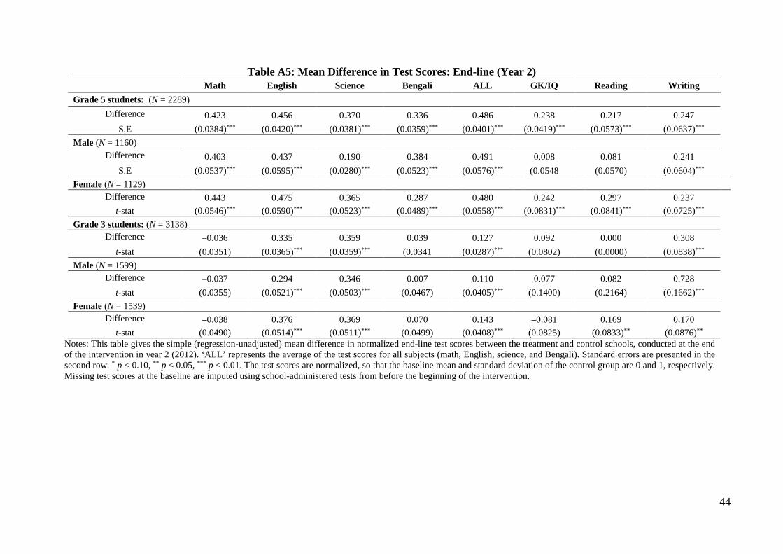
44

Table A5: Mean Difference in Test Scores: End-line (Year 2)

Math English Science Bengali ALL GK/IQ Reading Writing Grade 5 studnets: (N = 2289)

Difference 0.423 0.456 0.370 0.336 0.486 0.238 0.217 0.247 S.E (0.0384)*** (0.0420)*** (0.0381)*** (0.0359)*** (0.0401)*** (0.0419)*** (0.0573)*** (0.0637)***

Male (N = 1160) Difference 0.403 0.437 0.190 0.384 0.491 0.008 0.081 0.241

S.E (0.0537)*** (0.0595)*** (0.0280)*** (0.0523)*** (0.0576)*** (0.0548 (0.0570) (0.0604)*** Female (N = 1129)

Difference 0.443 0.475 0.365 0.287 0.480 0.242 0.297 0.237 t-stat (0.0546)*** (0.0590)*** (0.0523)*** (0.0489)*** (0.0558)*** (0.0831)*** (0.0841)*** (0.0725)***

Grade 3 students: (N = 3138) Difference –0.036 0.335 0.359 0.039 0.127 0.092 0.000 0.308

t-stat (0.0351) (0.0365)*** (0.0359)*** (0.0341 (0.0287)*** (0.0802) (0.0000) (0.0838)*** Male (N = 1599)

Difference –0.037 0.294 0.346 0.007 0.110 0.077 0.082 0.728 t-stat (0.0355) (0.0521)*** (0.0503)*** (0.0467) (0.0405)*** (0.1400) (0.2164) (0.1662)***

Female (N = 1539) Difference –0.038 0.376 0.369 0.070 0.143 –0.081 0.169 0.170

t-stat (0.0490) (0.0514)*** (0.0511)*** (0.0499) (0.0408)*** (0.0825) (0.0833)** (0.0876)** Notes: This table gives the simple (regression-unadjusted) mean difference in normalized end-line test scores between the treatment and control schools, conducted at the end of the intervention in year 2 (2012). ‘ALL’ represents the average of the test scores for all subjects (math, English, science, and Bengali). Standard errors are presented in the second row. * p < 0.10, ** p < 0.05, *** p < 0.01. The test scores are normalized, so that the baseline mean and standard deviation of the control group are 0 and 1, respectively. Missing test scores at the baseline are imputed using school-administered tests from before the beginning of the intervention.

45

Table A6: ITT Estimates with Controls: Midline Results, Year 1

(1) (2) (3) (4) (5) (6) Grade 4 Grade 5 Panel A Math English Science Bengali ALL CGPA Treatment Effect 0.305** 0.319** 0.182 0.308** 0.281** 0.219** (0.142) (0.156) (0.126) (0.117) (0.132) (0.105) Baseline Test Score 0.122*** 0.110*** 0.247*** 0.0400** 0.0499*** 0.00860* (0.0148) (0.0178) (0.0317) (0.0174) (0.00518) (0.00515) HH Characteristics Yes Yes Yes Yes Yes Yes School Characteristics Yes Yes Yes Yes Yes Yes Teacher Characteristics Yes Yes Yes Yes Yes Yes N 1582 1586 1585 1587 1587 1385 adj. R2 0.196 0.194 0.188 0.080 0.259 0.044 Panel B Male 0.253* 0.296* 0.186 0.289** 0.266** 0.426*** (0.140) (0.149) (0.130) (0.133) (0.128) (0.0941) Female 0.206 0.214 0.0755 0.248* 0.232 0.0600 (0.141) (0.185) (0.151) (0.126) (0.148) (0.123)

Notes: Panel A of this table reports the regression coefficients using Equation (2). The baseline test scores in the regressions are the pre-intervention test scores for each subject. ‘ALL’ indicates the mean test score for all subjects (math, English, science, and Bengali). The estimated coefficient of ‘treatment’ is given in the first row. For the male and female sub-samples, we report only the coefficient of ‘treatment’ separately. The test scores are normalized, so that the baseline mean and standard deviation of the control group are 0 and 1, respectively. Standard errors are clustered at the school level and are reported in parentheses. The regression includes child gender, parental and household characteristics, and teacher and school characteristics. * p < 0.10, ** p < 0.05, *** p < 0.01.

46

Table A7: ITT Estimates with Control: End-line Results, Year 2

(1) (2) (3) (4) (5) (6) (7) (8) Grade 5 Math English Science Bengali ALL GK/IQ Reading Writing Treatment Effect 0.425*** 0.344** 0.343*** 0.324*** 0.361*** 0.294** 0.226 0.184 (0.158) (0.159) (0.129) (0.114) (0.125) (0.144) (0.146) (0.143) Baseline Test Score 0.189*** 0.188*** 0.248*** 0.152*** 0.281*** 0.372*** 0.199*** 0.256** (0.0478) (0.0706) (0.0500) (0.0441) (0.0776) (0.0798) (0.0587) (0.126) N 1152 1152 1152 1152 1152 1091 1091 1091 adj. R2 0.103 0.069 0.116 0.082 0.142 0.140 0.098 0.057 Male 0.455** 0.276 0.285* 0.388*** 0.346** 0.386*** 0.179 0.0905 (0.200) (0.182) (0.143) (0.139) (0.146) (0.137) (0.158) (0.135) Female 0.403*** 0.427*** 0.398*** 0.274** 0.383*** 0.198 0.259 0.280 (0.138) (0.154) (0.130) (0.108) (0.117) (0.174) (0.166) (0.186) Grade 3 Treatment Effect –0.0846 0.348*** 0.312*** 0.0348 0.165* 0.0270 0.0590 0.313* (0.0746) (0.0903) (0.107) (0.101) (0.0839) (0.0960) (0.125) (0.160) Baseline Test Score 0.304*** 0.304*** 0.299*** 0.348*** 0.484*** 0.387*** 0.240*** 0.232*** (0.0336) (0.0346) (0.0393) (0.0364) (0.0446) (0.0504) (0.0461) (0.0754) N 1049 1049 1049 1049 1049 896 896 896 adj. R2 0.167 0.157 0.178 0.187 0.243 0.143 0.077 0.068 Male –0.0622 0.369*** 0.378*** –0.0159 0.176* 0.102 -0.0608 0.439** (0.0909) (0.110) (0.121) (0.106) (0.0913) (0.115) (0.142) (0.170) Female –0.0698 0.348*** 0.236* 0.0957 0.166 -0.0543 0.175 0.190 (0.0897) (0.112) (0.119) (0.121) (0.102) (0.120) (0.137) (0.171)

Notes: This table reports the regression coefficients using Equation (2). The baseline test scores in the regressions are the pre-intervention test scores for each subject. ‘ALL’ indicates the mean test score for all subjects (math, English, science, and Bengali). The estimated coefficient of ‘treatment’ is given in the first row. For the male and female sub-samples, we report only the coefficient of ‘treatment’ separately. The test scores are normalized, so that the baseline mean and standard deviation of the control group are 0 and 1, respectively. For GK/IQ, reading and writing, the test scores are normalized at the end-line, with a control mean and standard deviation of 0 and 1, respectively. Standard errors are clustered at the school level and reported in parentheses. As no baseline tests for GK/IQ, reading, and writing were conducted, we use the standardized ALL scores as baseline score for these regressions. The regression includes child gender, parental and household characteristics, and teacher and school characteristics. * p < 0.10, ** p < 0.05, *** p < 0.01.

47

Table A8: Numbers of Meetings and Gains in Test Scores at the End-line (treatment schools only) (1) (2) (3) (4) (5) (6) (7) (8) Math English Science Bengali ALL GK/IQ Reading Writing Grade 5 0.102*** 0.165*** 0.0943*** 0.109*** 0.130*** 0.0452 0.0346 0.100* (0.0261) (0.0375) (0.0295) (0.0221) (0.0268) (0.0374) (0.0298) (0.0513) Grade 3 0.114*** 0.155*** 0.154*** 0.130*** 0.114*** 0.0756 0.143*** 0.0675 (0.0259) (0.0338) (0.0304) (0.0413) (0.0259) (0.0523) (0.0280) (0.0522)

Notes: The sample includes all students from the treatment schools only. Standard errors are clustered at the school level and are reported in parentheses. The regression includes child gender, parental/household characteristics, as well as teacher and school characteristics. * p < 0.10, ** p < 0.05, *** p < 0.01.

48

Table A9: Heterogeneous Effects: Grade 3, Year 2 (1) (2) (3) (4) (5) (6) (7) (8) Math English Science Bengali All GK/IQ Reading Writing Panel A: Interactions with household characteristics Treatment school*covariate Age of head (above median) –0.0120 0.168 0.143 0.0942 0.0764 0.00907 0.112 –0.167 (0.150) (0.170) (0.124) (0.155) (0.140) (0.147) (0.134) (0.169) Household size (above median) 0.0757 0.0488 –0.132 0.0514 0.00474 –0.185 –0.134 0.226 (0.173) (0.211) (0.203) (0.168) (0.169) (0.194) (0.214) (0.241) Student gender (female = 1) –0.0319 –0.0157 –0.0468 0.0846 –0.000409 –0.141 0.230 –0.196 (0.113) (0.129) (0.115) (0.102) (0.0994) (0.146) (0.141) (0.139) Both parents primary educated –0.0569 –0.0187 –0.169 –0.104 –0.0844 –0.107 0.0368 0.187 (0.107) (0.121) (0.116) (0.103) (0.0929) (0.121) (0.143) (0.150) Income above log median –0.000713 –0.0705 –0.0937 –0.0638 –0.0399 –0.0466 –0.111 0.00706 (0.152) (0.167) (0.170) (0.148) (0.138) (0.139) (0.167) (0.199) Panel B: Interactions with school and teacher characteristics Treatment school*covariate Student–teacher ratio –0.000657 0.00463 –0.000574 0.00469 0.00165 –0.00319 0.00262 –0.00891 (0.00758) (0.00736) (0.00888) (0.00919) (0.00773) (0.0106) (0.0104) (0.0120) Years of teaching experience –0.00855 –0.00973 –0.0142 –0.0172 –0.0155 –0.00852 –0.00691 0.0118 (0.00949) (0.0123) (0.0128) (0.0115) (0.0113) (0.0114) (0.0122) (0.0164) Number of classrooms 0.159** 0.147** 0.139* 0.0959 0.175** 0.00586 0.107 –0.0254 (0.0635) (0.0718) (0.0710) (0.0783) (0.0726) (0.0741) (0.0986) (0.111) School is brick-built –0.119 0.174 –0.162 –0.169 0.0101 –0.0369 –0.135 0.467 (0.214) (0.251) (0.236) (0.289) (0.217) (0.239) (0.288) (0.495) School has electricity –0.0686 –0.127 –0.296 –0.319 –0.189 –0.251 0.00305 0.242 (0.171) (0.196) (0.215) (0.213) (0.177) (0.234) (0.274) (0.323)

Notes: The top panel of the regression also includes child gender, parental and household characteristics, while the bottom panel includes teacher and school characteristics. Age, household size, education, and income have been converted to binary variables for ease of interpretation of the magnitude of the estimates. They are defined if the value is above the median in the overall sample. Standard errors are clustered at the school level and are reported in parentheses. * p < 0.10, ** p < 0.05, *** p < 0.01.

49

Table A10: Heterogeneous Treatment Effects, Grades 4 and 5, Year 1

(1) (2) (3) (4) (5) (6) Math English Science Bengali All CGPA (grade 5) Panel A: Interactions with household characteristics Treatment school*covariate Age of head (above median) 0.00502 0.135 0.151 0.132 0.115 0.0164 (0.126) (0.112) (0.116) (0.121) (0.103) (0.117) Household size (above median) –0.0802 –0.0586 –0.0696 0.0610 –0.00206 0.0527 (0.153) (0.151) (0.160) (0.159) (0.135) (0.148) Student gender (female = 1) –0.0254 –0.0507 –0.0485 –0.0396 0.00179 –0.401*** (0.111) (0.116) (0.114) (0.112) (0.0926) (0.101) Both parents primary educated 0.0273 –0.138 –0.176 –0.170 –0.119 –0.0432 (0.105) (0.102) (0.105) (0.0944) (0.0897) (0.129) Income above log median 0.102 0.155 0.119 0.117 0.175 0.124 (0.112) (0.118) (0.122) (0.106) (0.0987) (0.117) Panel B: Interactions with school and teacher characteristics Treatment school*covariate Student–teacher ratio –0.00838 –0.00586 –0.00155 0.00732 0.00293 0.00694 (0.00863) (0.00930) (0.00701) (0.00846) (0.00731) (0.00715) Years of teaching experience –0.0124 –0.0180 –0.00830 –0.0158 –0.00872 –0.00746 (0.0162) (0.0151) (0.0167) (0.0154) (0.0148) (0.0127) Number of classrooms –0.00230 0.0192 0.0483 –0.0254 –0.0147 –0.0997 (0.100) (0.0873) (0.0816) (0.0826) (0.0813) (0.0606) School is brick-built 0.398 1.096** 0.535 0.373 0.689 0.446 (0.441) (0.463) (0.372) (0.408) (0.473) (0.296) School has electricity –0.352 –0.331 –0.563** –0.360 –0.412 0.0234 (0.309) (0.317) (0.268) (0.228) (0.287) (0.184) N 1586 1590 1589 1591 1591 1393 adj. R2 0.171 0.194 0.174 0.051 0.246 0.045

Notes: The top panel of the regression also includes child gender, parental and household characteristics, while the bottom panel includes teacher and school characteristics. Age, household size, education, and income have been converted to binary variables for ease of interpretation of the magnitude of the estimates. They are defined if the value is above the median in the overall sample. Standard errors are clustered at the school level and are reported in parentheses. * p < 0.10, ** p < 0.05, *** p < 0.01.

50

Table A11: Teacher Absences in Unannounced (Random) Visits Treatment Control Diff (T – C) S.E t-stat

Teacher Absences in 2011 (Year 1) April 0.12 0.09 0.03 0.031 1.03 May 0.07 0.08 –0.01 0.025 0.43 June 0.09 0.05 0.04 0.026 1.48 August 0.11 0.20 –0.09 0.033 2.74 Absence in all visits in 2011 0.39 0.42 –0.03 0.065 0.47

Teacher Absences in 2012 (Year 2) Feb 0.32 0.27 0.05 0.044 1.18 March 0.32 0.34 –0.02 0.046 0.39 April 0.21 0.23 –0.02 0.040 0.54 May 0.23 0.19 0.04 0.040 0.93 June 0.17 0.18 –0.01 0.037 0.22 July 0.13 0.18 –0.04 0.035 1.30 August 0.25 0.24 0.01 0.042 0.23 Sept 0.23 0.32 –0.09 0.043 2.13 Oct 0.19 0.33 –0.14 0.042 3.31 Absence in all visits in 2012 2.31 2.56 –0.25 0.146 1.70

Notes: The third column shows the difference between the treatment and control schools. The fourth and fifth columns show the standard errors and the (absolute value of) t-statistics of the difference. Statistically significant differences are given in bold.

Table A12: Teacher Efforts and Pedagogical Practices Treat Control Diff (T – C) Teaching practice in classrooms (% of teachers) Rely mainly on textbooks 25% 51% –26% Use real-life examples 70% 48% 22%

51

Table A13: Student Absences from classes in Year 1 and Year 2

Treat Control Diff (T – C) S.E t-stat Student Absences in 2011

June 2.12 1.66 0.46 0.099 4.61 July 1.65 1.68 –0.03 0.077 0.39 August 0.77 1.37 –0.60 0.052 11.63 September 0.82 1.35 –0.53 0.057 9.30

Total number of days absent in these months Male 5.22 6.15 –0.93 0.315 2.95 Female 5.51 5.94 –0.43 0.326 1.32

Student Absences in 2012 March 1.00 1.26 –0.26 0.044 5.87 April 1.01 1.25 –0.23 0.047 4.97 May 0.87 1.01 –0.13 0.035 3.82 June 1.14 1.35 –0.21 0.047 4.40 July 1.46 1.43 0.03 0.047 0.59 August 0.63 0.60 0.03 0.024 1.10 September 1.32 1.38 –0.06 0.038 1.59 October 1.08 1.07 0.01 0.032 0.35 November 1.16 1.12 0.03 0.032 1.00

Total number of days absent in these months Male 13.48 13.02 0.46 0.341 1.34 Female 13.01 12.45 0.56 0.331 1.71

Notes: The third column shows the differences between the treatment and control schools. The fourth and fifth columns show the standard errors and the (absolute value of) t-statistics of the difference. Statistically significant differences are given in bold.

Table A14: Parents’ evaluations of Parent–Teacher Meetings Only for treatment schools % of parents Do you think that the parent meetings help to improve a child’s study? 93.36 Do you think that there should be monthly parent meetings in school? 91.03

52

Appendix 2 (Figures)

Figure A1A: Numbers of Meetings Attended in Year 1, by Gender of the Children (in %)

Figure A1B: Numbers of Meetings Attended in Year 2, by Gender of the Children (in %)

Note: Figure shows percentage of parents attended the number of meetings in year 1 (A1A) and year 2 (A1B) of the intervention by the gender of the child.

0

5

10

15

20

25

0 1 2 3 4 5

BOY

GIRL

0

5

10

15

20

25

0 1 2 3 4 5 6 7 8

BOY

GIRL

53

Figure A2A: Attendance at Meetings by Mothers or Fathers (others) in Year 1 (in %)

Figure A2B: Attendance at Meetings by Mothers or Fathers (others) in Year 2 (in %)

Note: Figure shows percentage of meetings attended by either mother or father among those attended in year 1 (A2A) and year 2 (A2B).

10

20

30

40

50

60

70

80

90

June July August September October

Mother

Father

10

20

30

40

50

60

70

80

90

March April May June July August September October

Mother

Father

54

Figure A3A: Numbers of Meetings Attended by Parents in Year 1

Figure A3B: Numbers of Meetings Attended by Parents in Year 2 Note: Figure shows the total number of meetings attended by percentage of parents in year 1 (A3A) and year 2 (A3B) of the intervention.

0.0

5.1

.15

.2.2

5P

erce

ntag

e of

par

ents

0 1 2 3 4 5Number of meetings

0 .0

5 .1

.1

5 .2

Pe

rcen

tage

of P

aren

ts

0 2 4 6 8 Number of Meetings

55

Figure A4: Distribution of Cumulative GPA Test Scores in Year 1

Note: Figure shows GPA test scores distribution of treatment and control school children of grade 5 students at the end of year 1 of the intervention.

0.1

.2.3

.4.5

Den

sity

-2 -1 0 1 2x

Control GPA (standardized) Treatment GPA (standardized)

56

Figure A5: Parental Presence at Meetings by the Distribution of the Students’ Baseline Test Scores

Note: Figure represents the percentages of meetings that parents attended, based on their children’s baseline test score distributions, by a child grade in year 2.

0.4

0.5

0.6

0.7

0.8

Bottom Third Middle Third Top Third

% o

f all

mee

tings

atte

nded

by

pare

nts

Students' baseline rank

grade 3

grade 5

57

Appendix 3

Sample Report Card School Address:

Village Name Student Address School Name Student Name Upazila/Thana Parent’s Name District Class Mobile/Telephone Class Roll

Student’s Date of Birth: Day………./Month…………/Year…………….. Guardian Father = 1 Mother = 2

Subject Code Baseline Test, 2011

March April May June July August September October November

Bangla 1 English 2 Mathematics 3 Science 4 Social science 5 General science 6

Other information:

Presence of student (days) March April May June July August September October November Total Total working days (days) Absent (days) Guardian’s Presentation (code)*

* For treatment schools only; this option was not available for report cards in control schools. Code: 1 = Father; 2 = Mother; 3 = Brother/Sister; 4 = Other; 9 = Absent.