Parent-Child Information Frictions and Human Capital Investment:Evidence from a Field Experiment∗

Peter Bergman†

This paper studies information frictions between parents and their children, and howthese affect human capital investments. I provide detailed, biweekly information to a ran-dom sample of parents about their child’s missed assignments and grades and find parentshave upwardly-biased beliefs about their child’s effort. Providing additional information at-tenuates this bias and improves student achievement. Using data from the experiment, I thenestimate a persuasion game between parents and their children that shows the treatmenteffect is due to a combination of more accurate beliefs and reduced monitoring costs. Theexperimental results and policy simulations from the model demonstrate that improving thequality of school reporting or providing frequent information to parents about their child’seffort in school can produce gains in achievement at a low cost.

JEL Codes: I20, I21, I24.

∗I am grateful to Adriana Lleras-Muney, Pascaline Dupas and Karen Quartz for theiradvice and support. I also thank James Heckman and five referees for their detailed feedbackand suggestions, as well as helpful comments from Matthew Baird, Sandra Black, Pierre-Andre Chiappori, Jon Guryan, Navin Kartik, Day Manoli, Magne Mogstad, Paco Martorell,Robert McMillan, Sarah Reber, Todd Rogers and Mitchell Wong. Seminar participantsat AEFP, Case Western University, CESifo, the CFPB, Mathematica, NBER Educationmeeting, University of Toronto, RAND, Teachers College, Columbia University, UC Berkeley,the University of Chicago and UCLA gave valuable suggestions as well. Andrew Kosenko,Chaoyan Zhu and Danna Kang Thomas provided excellent research assistance. All errorsare my own.†Teachers College, Columbia University, 525 W. 120th Street New York, New York 10027

E-mail: bergman@tc.columbia.edu

I Introduction

Most models of human capital development assume that parents have full control over in-

vestments in their children’s skills. While this assumption is plausible at early stages of child

development, it is likely less so as children get older and develop greater agency (Cunha and

Heckman, 2007; Heckman and Mosso, 2014). If parent and child preferences over schooling

diverge, this agency problem complicates the ability of parents to foster their child’s skills.

Specifically, parents need to motivate and track their child’s progress in school but they

cannot rely on their children to communicate the relevant information, as a child may have

an incentive to manipulate it.

This paper uses a field experiment in combination with a structural modeling approach

to understand potential information frictions between parents and their children and the

extent to which such frictions can be resolved by providing information to parents about

their children’s academic progress. To measure the effects of providing additional informa-

tion, I conducted an experiment at a school in a low-income area of Los Angeles. Parents or

guardians were randomly selected to receive additional information about their child’s aca-

demic progress. This information consisted of emails, text messages and phone calls listing

students’ missing assignments and grades several times a month over a six-month period.

The information provided was detailed in nature: messages contained the class, assignment

names, problems and page numbers of the missing work whenever possible. Course grades

were sent to families every five to eight weeks. To quantify the effects of the treatment on

student effort, achievement and parental behaviors, I gathered administrative data on assign-

ment completion, work habits, cooperation, attendance and test scores. Parent and student

surveys were also conducted immediately after the school year ended to provide additional

data about each family’s response.

The reduced-form results uncover several important information problems. First, I show

that parents have upwardly-biased beliefs about their child’s effort in school: when asked

1

to estimate how many assignments their child has missed in math class, parents vastly

understate. The size of this bias is negatively and significantly associated with student

achievement and the information treatment attenuates this bias. Second, more information

increases the intensity of parental monitoring and incentives, and increases inputs such as

student effort. Parents in the treatment group contacted the school 83% more often than the

control group and parent-teacher conference attendance increased by 53%. Third, schoolwork

is consistently at the top of parents’ mind: parents in both the treatment and control groups

ask their child whether they have completed their schoolwork nearly five times per week,

on average. However, parents rarely attend meetings with teachers to discuss their child’s

academics (15% attended parent-teacher conferences in the last semester) and neither parents

nor schools reach out to each other often (median parent contact is 1.5 times per semester).

In terms of achievement, reducing these information problems can potentially produce

gains on a par with education reforms such as the introduction of high-quality charter schools.

GPA increased by .19 standard deviations. There is evidence that test scores for math in-

creased by .21 standard deviations, though there was no gain for English scores (.04 standard

deviations). These effects are driven by several changes in students’ inputs: assignment com-

pletion increased by 25% and the likelihood of unsatisfactory work habits and cooperation

decreased by 24% and 25%, respectively. Classes missed by students decreased by 28%. For

comparison, the Harlem Children’s Zone increased math scores and English scores by .23

and .05 standard deviations and KIPP Lynn charter schools increased these scores .35 and

.12 standard deviations (Dobbie and Fryer, 2010; Angrist et al., 2010).

Based on these reduced-form results, I estimate a model of parent-child interactions as

a game of strategic-information disclosure, or a persuasion game (Dye, 1985; Shin, 1994).

This is a signaling game with incentives and parental monitoring combined with potentially

biased parent beliefs about their child’s effort. Children choose to exert effort in school or

not and may offer parents verifiable reports regarding their effort, for instance via graded

papers or report cards, or choose to hide this information. Parents have beliefs over their

2

child’s cost of effort and the probability of a verifiable report existing. The latter breaks

the unraveling result (Grossman, 1981; Milgrom, 1981) in which parents simply assume the

worst in the absence of information disclosure; this is particularly pertinent to low-achieving

schools, where parents report school communication is often poor (Bridgeland et al., 2008).

Parents may monitor effort, for example by going to the school to speak with teachers to

obtain a verifiable report, and take away privileges if children are exerting inadequate effort

with respect to parental preferences. I present identifying conditions that map observed

actions into unique equilibria and I estimate the model using maximum likelihood.

The model serves two purposes. First, while the experimental variation alone cannot

disentangle the channels through which the treatment influenced information problems and

student effort, by estimating the model I can decompose the treatment effect into changes

due to monitoring costs versus changes due to revised parental beliefs. Understanding these

mechanisms has implications for when and how additional information will be effective. I

find that a substantial portion of the treatment effect can be attributed to changes in parents’

beliefs (42%) and reductions in monitoring costs (54%).

Second, I use the model to consider alternative policies that could be used to reduce infor-

mation frictions. Rather than reducing monitoring costs, I consider a policy that improves

school reporting. Simulating the effect of improving school reporting shows this policy can

improve student effort as well, though by half the magnitude of providing additional infor-

mation. Nonetheless, encouraging teachers to grade papers and enter them into gradebooks

may be more scalable and less controversial than alternative policies to improve student

achievement.

These costs are important because alternative policies aimed at improving the achievement

of adolescents can be expensive. They often rely on financial incentives, either for teachers

(Springer et al., 2010; Fryer, 2011), for students (Angrist and Lavy, 2002; Bettinger, 2008;

Fryer, 2011) or for parents (Miller, Riccio and Smith, 2010).1 Providing financial incentives

1Examples of other information-based interventions in education include providing families information describing student

3

for high school students cost $538 per .10 standard-deviation increase, excluding adminis-

trative costs (Fryer, 2011). If teachers were to provide additional information to parents

as in this study, the cost per student per .10 standard-deviation increase in GPA or math

scores would be $156 per child per year. Automation could reduce this to less than $10 per

student.

An important question related to costs is how much parents might be willing to pay to

reduce these information problems. My study does not address this question, but Bursztyn

and Coffman (2012) use a lab experiment with low-income families in Brazil to show parents

are willing to pay substantial amounts of money for information on their child’s attendance.

While this paper shows that an intensive information-to-parents service can potentially

produce gains to student effort and achievement, its policy relevance depends on how well it

scales. Large school districts such as Los Angeles, Chicago, and Baltimore have purchased

systems that make it easier for teachers to improve communication with parents by post-

ing grades online, sending automated emails regarding grades, or text messaging parents

regarding schoolwork. The availability of these services prompts questions about their us-

age, whether teachers update their grade books often enough to provide information, and

parental demand for this information. This paper discusses but does not address these

questions empirically.2

The rest of the paper proceeds as follows. Sections II and III describe the experimen-

tal design and the estimation strategy. Sections IV and V show reduced-form impacts on

achievement and parent and child behaviors. Section VI presents the model, estimation

procedure and results. Section VII concludes with a discussion of external validity and

cost-effectiveness.

achievement at surrounding schools (Hastings and Weinstein, 2008; Andrabi, Das and Khwaja 2009), parent outreach programs(Avvisati et al., 2013), providing principals information on teacher effectiveness (Rockoff et al., 2010) and helping parents fillout financial aid forms (Bettinger et al., 2009).

2See Bergman (2016) on the low-parental usage of online information about student academic progress.

4

II Background and Experimental Design

A Background

I conducted the experiment at a K-12 school during the 2010-2011 school year. This school is

part of Los Angeles Unified School District (LAUSD), which is the second largest district in

the United States. The district has graduation rates similar to other large urban areas and is

low performing according to its own proficiency standards: 55% of LAUSD students graduate

high school within four years, 25% of students graduate with the minimum requirements to

attend California’s public colleges, 37% of students are proficient in English-Language Arts

and 17% are proficient in math.3

The school is in a low-income area with a high percentage of minority students: 90% of

students receive free or reduced-price lunch, 74% are Hispanic and 21% are Asian. Com-

pared to the average district scores above, the school performs less well on math and English

state exams; 8% and 27% scored proficient or better in math and English respectively. 68%

of teachers at the school are highly qualified, defined as being fully accredited and demon-

strating subject-area competence.4 In LAUSD, the average high school is 73% Hispanic, 4%

Asian and 89% of teachers are highly qualified.5

The school context has several features that are distinct from a typical LAUSD school.

The school is located in a large building complex designed to house six schools and to serve

4,000 students living within a nine block radius. These schools are all new, and grades

K-5 opened in 2009. The following year, grades six through eleven opened. Thus in the

2010-2011 school year, the sixth graders had attended the school in the previous year while

students in grades seven and above spent their previous year at different schools. Families

living within the nine-block radius were designated to attend one of the six new schools but

3This information and school-level report cards can be found online at http://getreportcard.lausd.net/reportcards/reports.jsp.4Several papers have shown that observable teacher characteristics are uncorrelated with a teacher’s effect on test scores

(Aaronson et al., 2008; Jacob and Lefgren, 2008; Rivken et al., 2005). Buddin (2010) shows this result applies to LAUSD aswell.

5This information is drawn from the district-level report card mentioned in the footnote above.

5

were allowed to rank their preferences for each. These schools are all pilot schools, which

implies they have greater autonomy over their budget allocation, staffing, and curriculum

than the typical district school.6

B Experimental Design

The sample frame consisted of all students in grades six through eleven enrolled at the school

in December of 2010. The sample was stratified along indicators for being in high school,

having had a least one D or F on their mid-semester grades, having a teacher think the

service would helpful for that student, and having a valid phone number.7 Students were

not informed of their family’s treatment status nor were they told that the treatment was

being introduced. Teachers knew about the experiment but were not told which families

received the additional information. Interviews with students suggest that several students

discussed the messages with each other. Due to contamination in the middle school sample,

I study the stratified sample of 306 students in high school.8

The focus of the information treatment was missing assignments, which included home-

work, classwork, projects, essays and missing exams. Each message contained the assignment

name or exam date and the class it was for whenever possible. For some classes, this name

included page and problem numbers; for other classes it was the title of a project, worksheet

or science lab. Overwhelmingly, the information provided to parents was negative—nearly

all about work students did not do. The treatment rule was such that a single missing as-

signment in one class was sufficient to warrant a message home. All but one teacher accepted

late work for at least partial credit. Parents also received current-grades information three

times and a notification about upcoming final exams.

6The smaller pilot school system in Los Angeles is similar to the system in Boston. Abdulkadiroglu et al.(2011) find that the effects of pilot schools on standardized test scores in Boston are generally small and not sig-nificantly different from traditional Boston public schools. For more information on LAUSD pilot schools, seehttp://publicschoolchoice.lausd.net/sites/default/files/Los%20Angeles%20Pilot%20Schools%20Agreement%20%28Signed%29.pdf.

7The validity of the phone number was determined by the school’s automated-caller records.8Middle school teachers had a school employee replicate the treatment for all students, treatment and control. This employee

called parents regarding missing assignments and set up parent-teacher conferences in addition to the school-wide conferences.This contamination began four or five weeks after the treatment started and makes interpreting the results for the middle schoolsample difficult. See the appendix for all results from the middle school sample.

6

The information provided to parents came from teacher grade books gathered weekly from

teachers. 14 teachers were asked to participate by sharing their grade books so that this

information could be messaged to parents. The goal was to provide additional information

to parents twice a month if students missed work. The primary constraint on provision was

the frequency at which grade books were updated. Updated information about assignments

could be gathered every two-to-four weeks from nine of the fourteen teachers. Therefore these

nine teachers’ courses were the source of information for the messages and the remaining

teachers’ courses could not be included in the treatment. These nine teachers were sufficient

to have grade-book level information on every student.

The control group received the default amount of information the school provided. This

included grade-related information from the school and from teachers. Following LAUSD

policy, the school mailed home four report cards per semester. One of these reports was

optional—teachers did not have to submit grades for the first report card of the semester.

The report cards contained grades, a teacher’s comment for each class, and each teacher’s

marks for cooperation and work habits. All school documents were translated into Spanish

and Korean, and the school employed several Korean and Spanish translators. Parent-teacher

conferences were held once per semester. Attendance for these conferences was very low for

the high school (roughly 15% participation). Teachers could also provide information to

parents directly. At baseline, most teachers had not contacted any parents. No teacher had

posted grades on the Internet though two teachers had posted assignments.

Figure 1 shows the timeline of the experiment and data collection. Baseline data was col-

lected in December of 2010. That same month, contact numbers were culled from emergency

cards, administrative data and the phone records of the school’s automated-calling system.

In January 2011, parents in the treatment group were called to inform them that the school

was piloting an information service provided by a volunteer from the school for half the

parents at the school. Parents were asked if they would like to participate, and all parents

consented, which implies no initial selection into treatment. These conversations included

7

questions about language preference, preferred method of contact—phone call, text message

or email—and parents’ understanding of the A-F grading system. Most parents requested

text messages (79%), followed by emails (13%) and phone calls (8%).9

The four mandatory grading periods after the treatment began are also shown, which

includes first-semester grades. Before the last progress report in May, students took the Cal-

ifornia Standards Test (CST), which is a state-mandated test that all students are supposed

to take.10 Surveys of parents and students were conducted over the summer in July and

August. Lastly, course grades from February 2012, more than one year after the experiment

began and seven months after its conclusion, were also collected the following school year.

Notifications began in early January of 2011 and were sent to parents of middle school

students and high school students on alternating weeks. This continued until the end of

June, 2011. A bar graph above the timeline charts the frequency of contact with families

over six months. The first gap in messages in mid February reflects the start of the new

semester and another gap occurs in early April during spring vacation. This graph shows

there was a high frequency of contact with families.

III Data and Empirical Strategy

A Baseline Data

Baseline data include administrative records on student grades, courses, attendance, race,

free-lunch status, English-language skills, language spoken at home, parents’ education levels

and contact information. There are two measures of GPA at baseline. For 82% of students

their cumulative GPA prior to entering the school is also available. The second measure

of GPA is calculated from their mid-semester report card, which was two months before

the treatment began. At the time of randomization only mid-semester GPA was available.

Report cards contain class-level grades and teacher-reported marks on students’ work habits

9A voicemail message containing the assignment-related information was left if no one picked up the phone.10Students with special needs can be exempted from this exam.

8

and cooperation. As stated above, there is an optional second-semester report card, however

the data in this paper uses mandatory report cards to avoid issues of selective reporting of

grades by teachers.

Teachers were surveyed about their contact with parents and which students they thought

the information treatment would be helpful for. The latter is coded into an indicator for at

least one teacher saying the treatment would be helpful for that student.

B Achievement-Related Outcomes

Achievement-related outcomes are students’ grades, standardized test scores and final exam

or project scores from courses. Course grades and GPA are drawn from administrative

data on report cards. There are four mandatory report cards available after the treatment

began, but only end-of-semester GPA and grades remain on a student’s transcript. There

are two sets of end-of-semester grades: transcript grades obtained during the school year in

which the experiment was conducted and transcript grades obtained seven months after the

experiment concluded. Final exam and project grades come from teacher grade books and

are standardized by class.

The standardized test scores are scores from the California Standards Tests. These tests

are high-stakes exams for schools but are low stakes for students. The math exam is sub-

divided by topic: geometry, algebra I, algebra II and a separate comprehensive exam for

students who have completed these courses. The English test is different for each grade.

Test scores are standardized to be mean zero and standard deviation one for each different

test within the sample.

C Effort-Related Measures

Measures of student effort are student work habits, cooperation, attendance and assignment

completion. Work habits and cooperation have three ordered outcomes: excellent, satisfac-

tory and unsatisfactory. There is a mark for cooperation and work habits for each class and

9

each grading period, and students typically take seven to eight classes per semester. Assign-

ment completion is coded from the teacher grade books. Missing assignments are coded into

indicators for missing or not.

There are three attendance outcomes. Full-day attendance rate is how often a child

attended the majority of the school day. Days absent is a class-level measure showing how

many days a child missed a particular class. The class attendance rate measure divides this

number by the total days enrolled in a class.

D Parental Investments and Family Responses to Information

Telephone surveys were conducted to examine parent and student responses to the inter-

vention not captured by administrative data. For parents, the survey asked about their

communication with the school, how they motivated their child to get good grades, and

their perceptions of information problems with their child about schoolwork. Parent-teacher

conference attendance was obtained from the school’s parent sign-in sheets. The student

survey asked about their time use after school, their communication with their parents and

their valuations of schooling.11

The parent and student surveys were conducted after the experiment ended by telephone.

52% of middle-school students’ families and 61% of high-school students’ families responded

to the telephone survey.12 These response rates are analyzed in further detail below.

To reduce potential social-desirability bias—respondents’ desire to answer questions as

they believe surveyors would prefer—the person who sent messages regarding missing assign-

ments and grades did not conduct any surveys. No explicit mention about the information

service was made until the very end of the survey.

All variables, their observation counts, and their source is summarized in appendix Table

A.1.11Students were also asked to gauge how important graduating college and high school is to their parents, but there was very

little variation in the responses across students so these questions are omitted from the analysis.12The school issued a paper-based survey to parents at the start of the year and the response rate was under 15%. An

employee of LAUSD stated that the response rates for their paper-based surveys is 30%.

10

E Attrition, Non Response, Missing CST Scores

Of the 306 students in the sample, 279 remained throughout the school year. 8% of attriters

were in the treatment group and 6% were in the control group.13 The most frequent cause

of attrition is transferring to a different school or moving away. Students who left the school

are lower performing than the average student. The former have significantly lower baseline

GPA and attendance as well as poorer work habits and cooperation. Table A.2 shows these

correlates in further detail. Attrition is more substantial for the longer-run followup, seven

months after the conclusion of the intervention: 14% of students leave the sample between

the end of the school year (June, 2011) to the end of the semester followup (February, 2012).

This is not correlated with treatment status, however (Table A.3).

Just over one third of parents did not respond to the survey.14 Table A.4 shows nonre-

sponse correlates. Nonresponse is uncorrelated with treatment status for both children and

parents. However, if those who did not respond differ from the typical family, then results

based on the surveys may not be representative of the school population. This is true, as a

regression of an indicator for non response on baseline characteristics shows the latter are

jointly significant (results not shown). Nonetheless, the majority of families responded and

provide insight into how they responded to the additional information.

Lastly, many students did not take the California Standards Test. 8% of scores are missing

for math and 7% of scores are missing for English. These tests were taken on different days.

Table A.5 in the appendix shows the correlates of missing scores. Baseline controls are added

for each of the first three columns with an indicator for missing math scores as the dependent

variable. The remaining three columns perform the same exercise for missing English scores.

The treatment is negatively and significantly associated with missing scores. The potential

bias caused by these missing scores is discussed further in the results section on test scores.

13This degree of attrition is not unusual in this area. Another study at a Los Angeles area school documented 7% attritionfrom the start to the end of the school year, and substantially more attrition from spring to fall (Dudovitz et al., 2013).

14For comparison, LAUSD has said their non-response rate for parent surveys is roughly double this number.

11

F Descriptive Statistics

In practice, the median treatment-group family was contacted 10 times over six months.

Mostly mothers were contacted (62%), followed by fathers (24%) and other guardians or

family members (14%). 60% of parents asked to be contacted in Spanish, 32% said English

was acceptable, and 8% wanted Korean translation.

Table 2 presents baseline-summary statistics across the treatment and the control groups.

Panel A contains these statistics for the original sample while Panel B excludes attriters

to show the balance of the sample used for estimations. Measures of works habits and

cooperation are coded into indicators for unsatisfactory or not and excellent or not. Of the 13

measures, one difference—the fraction of female students—is significantly different (p-value

of .078) between the treatment and control group in Panel A. All results are robust to adding

gender as a control. Work habits and students’ cumulative GPA from their prior grades are

better (but not significantly) for the control group than the treatment group. Panel B shows

that baseline GPA is .06 points higher for the control group than the treatment group in

the sample used for analysis, and as shown below, results are sensitive to this control. One

concern with this baseline difference is mean reversion, however students’ prior GPA, which

is a cumulative measure of their GPA over several years, also shows the treatment group is

lower achieving than the control group. In addition, GPA for the control group is highly

persistent from the end of the first semester to the end of the second semester. A regression

of the latter on the former yields a coefficient near one.15

G Empirical Strategy

The reduced-form analyses estimate intent-to-treat effects. Families in the treatment group

may have received fewer or no notifications because their child has special needs (13 fami-

lies); the guidance counselor requested them removed from the list due to family instability

15Mean reversion does occur between students’ prior GPA and their baseline GPA, however this reversion does not differ bytreatment status (results available on request).

12

(two families); or the family speaks a language other than Spanish, English or Korean (two

families). All of these families are included in the treatment group.

To measure the effect of additional information on various outcomes, I estimate the fol-

lowing

yi = α + β ∗ Treatmenti +X ′iγ + εi (1)

Control variables in X include baseline GPA and cumulative GPA from each student’s prior

school, grade indicators and strata indicators. The results are robust to various specifications

so long as a baseline measure of GPA is controlled for, which most likely makes a difference

due to the .06 point difference at baseline.

I estimate equation 1 with GPA as a dependent variable. To discern whether there were

any differential effects by subject or for “targeted” classes—those classes for which a teacher

shared a grade book in a timely fashion—I also use class grades as a dependent variable.16

This regression uses the same controls as 1 above but the standard errors are clustered at

the student level.17 End-of-semester grades are coded on a four-point scale to match GPA

calculations.18

Similar to class grades, there is a work habit mark and a cooperation mark for each

student’s class as well. I estimate the effect of additional information on these marks using

an ordered-Probit model that pools together observations across grading periods and clusters

standard errors at the student level. The controls are the same as above with additional

grading-period fixed effects. I report marginal effects at the means, but the average of the

marginal effects yields similar results.

Effects on full-day attendance and attendance at the classroom level use the same speci-

fication and controls as the specifications for GPA and class grades, respectively.

16Recall that only nine of the 14 teachers updated their grade books often enough so that assignment-related informationcould be provided to parents. The class-grades regression estimates whether treated students in those nine teachers’ classesshowed greater gains than the classes of teachers who did not update grades often enough to participate.

17Clustering at the teacher level or two-way clustering by teacher and student yield marginally smaller standard errors.18A is coded as 4, B as 3, C as 2, D as 1 and F as 0.

13

The number of observations changes depending on the particular outcome being studied.

For instance, students take more than one course each term, so when examining heterogeneity

across course subject there is more than one observation per child. This is also true for class

exams, in which the same student may take exams in multiple classes, and is also true

for class attendance and class-level behaviors. When applicable, tables will show both the

number of observations and the number of students used in the analysis.

IV Results

The Effect of the Treatment on School-to-Parent Contact

Table 3 assesses the effect of the treatment on survey measures of school-to-parent contact.

Parents were asked how often the school contacted them during the last month of school

regarding their child’s grades or schoolwork. During this time all parents had been sent a

progress report about their child’s grades. The first column shows how much more often the

treatment group was contacted by the school than the control group, controlling for baseline

GPA and cumulative GPA from students’ prior schools.19 The treatment increased contact

from the school regarding their child’s grades and schoolwork by 187% relative to the control

group. The dependent variable in the second column measures the fraction of people that

were contacted by the school more than once. This fraction increases by 158% relative to

the control group. The treatment had large effects on both the extensive margin of contact

and the intensive margin of contact from the school regarding student grades.

Effects on Achievement Measures

A GPA

Figure 3 tracks average GPA in the treatment and control groups over time. The red vertical

line indicates when the treatment began, which is about one month before the first semester

19The results without controls are extremely similar.

14

ended in mid February. There is a steady decrease in GPA for the control group after

the first semester ends in February followed by a spike upward during the final grading

period. The treatment group does not experience this decline and still improves in the final

grading period. Teachers reported that students work less in the beginning and middle of

the semester and “cram” during the last grading period to bring up their GPA, which may

negatively affect learning (Donovan, Figlio and Rush, 2006).

The regressions in Table 4 reinforce the conclusions drawn from the graphs described

above. Column (1) shows the effect on GPA with no controls. The increase is .15 and is

not significant, however the treatment group had a .06 point lower GPA at baseline. Adding

a control for baseline GPA raises the effect to .20 points and is significant at the 5% level

(column (2)). The standard errors decrease by 35%. The third column adds controls for

GPA from students’ prior schools and grade level indicators. The treatment effect increases

slightly to .23 points. The latter converts to a .19 standard deviation increase in GPA over

the control group.

The results in Table 5 are estimates of the treatment effect on class grades. Column

(1) shows this effect is nearly identical to the effect on final GPA.20 Column (2) shows the

effect on targeted classes—those classes for which a teacher was asked to participate and

that teacher provided a grade book so that messages could be sent home regarding missing

work. This analysis is underpowered, but the interaction term is positive and not significant

(p-value equals .16). Columns (3) and (4) show that math classes had greater gains than

English classes (p-values equal .11 and .85, respectively). This effect disparity coincides with

the difference in effects shown later for standardized tests scores.

Even though grading standards are school specific, the impact on GPA is important.

In the short run, course grades in required classes determine high school graduation and

higher education eligibility. In the longer run, several studies find that high school GPA is

the best predictor of college performance and attainment (for instance Geiser and Santelices,20The similarity in effects between this unweighted regression on individual grades and the regression on GPA is because

there is small variation in the number of classes students take.

15

2007). GPA is also significantly correlated with earnings even after controlling for test scores

(Rosenbaum, 1998; French et al., 2010). 21

B Final Exams, Projects and Standardized Test scores

Additional information causes exam and final project scores to improve by .16 standard

deviations (significant at the 5% level, Table 6). However, teachers enter missing finals as

zeros into the grade book. On average, 18% percent of final exams and projects were not

submitted by the control group. The effect on the fraction of students turning in their final

exam or project is large and significant. Additional information reduces this fraction missing

by 42%, or 7.5 percentage points.

Ideally, state-mandated tests are administered to all students, which would help separate

out the treatment effect on participation from the effect on their score. Unfortunately, many

students did not take these tests, and as shown above, missing a score is correlated with

treatment status and treatment-control imbalance.22 To account for this potential bias, the

effects on math and English test scores are shown with a varying number of controls. The first

and fourth columns in Table 7 control only for baseline GPA. The effect on math and English

scores are .08 and -.04 standard deviations respectively. Columns (2) and (5) add controls

for prior test scores, demographic characteristics and test subject. The treatment effect on

math scores is .21 standard deviations, but remains near zero for English scores. Finally,

if the treatment induces lower performing students to take the test, then those with higher

baseline GPA might be less affected by this selection. This means we might see a positive

coefficient on the interaction term between baseline GPA and the treatment. Columns (3)

and (6) add this interaction term. While the interaction term is small for English scores,

for math scores it implies that someone with the average GPA of 2.01 has a .20 standard

21One caveat, however, is that the mechanisms that generate these correlations may differ from the mechanisms underlyingthe impact of additional information on GPA.

22See the Appendix section on sample selection and test scores for further analysis of missing test takers; Table A.9 suggeststhat this attrition downwardly biases results.

16

deviations higher math score due to the additional information provided to their parents.23

This disparity between math and English gains is not uncommon. Bettinger (2010) finds

financial incentives increase math scores but not English scores and discusses several previous

studies (Reardon, Cheadle, and Robinson, 2008; Rouse, 1998) on educational interventions

that exhibit this difference as well. There are three apparent reasons the information inter-

vention may have had a stronger effect on math than English. First, the math teachers in

this sample provided more frequent information on assignments that allowed more messages

to be sent to parents. Potentially, this frequency might mean students fall less behind.24

Second, 30% of students are classified as “limited-English proficient,” which means they are

English-language learners and need to pass a proficiency test three years in a row to be

reclassified. Looking at class grades, these students tend to actually perform better in En-

glish classes, though interacting the treatment with indicators for language proficiency and

English classes yields a large and negative coefficient (results not shown). In contrast, this

coefficient is negative but 75% smaller when the interaction term includes an indicator for

math classes rather than English classes. This means that the treatment effect for students

with limited English skills is associated with smaller gains for English than math, which

may in part drive the disparity in effects. Lastly, math assignments might provide better

preparation for the standardized tests compared to English assignments if they more closely

approximate the problems on the test.

V Parent and Child Behaviors

Impacts on Parental Beliefs

To study the impact of the additional information on parents’ beliefs about their child’s effort,

I discretize parents’ estimate of their child’s missing assignments into the four categories in

23This marginal effect at the mean is significant at the 5% level.24This theory is difficult to test since there is no within-class variation in grade-book upkeep or message frequency conditional

on missing an assignment.

17

Table 8 and I estimate a multinomial-Logit model. Panel A show that the treatment causes

parents to revise their beliefs. There is a large, statistically significant reduction in the

probability of responding “I don’t know,” and a large, statistically significant increase in the

probability responding their child has missed 3-5 assignments. There are no changes in the

other categories. Second, the treatment impacts the size of the bias. Panel B shows results

from a linear model for effects on the continuous “Difference from Truth” variable. The

treatment significantly reduces the magnitude of the bias. This revision is particularly stark

for parents of students with low baseline GPA, as indicated in the second column of Table

8.

This result is corroborated by results in Panel B in the third column, which shows that

parents lacked awareness of the information problems with their child regarding school work.

This column reports the answers to the question: does your child not tell you enough about

his or her school work or grades? Parents in the treatment group are almost twice as likely

to say yes as parents in the control group.

A How Parents Used the Additional Information

A change in parental beliefs and a reduction in monitoring costs may cause to parents to

increase the use of monitoring and incentives. Panel A of Table 9 reflects impacts on measures

of parental monitoring. Over the last semester, parents in the treatment group were 85%

more likely to contact the school regarding their child’s schoolwork or grades, and this is

corroborated by the school’s data on parent-teacher conference attendance, which increased

by 53%. Parents regularly consider their child’s schoolwork; parents in the control group

ask their children about completing their work nearly five times per week. There is little

impact on this measure: the last column shows the coefficient on the treatment is negative

and insignificant.

Panel B of Table 9 shows how parents interacted with their children. In terms of incentives,

parents were asked how many privileges they took away from their child in the last month

18

of school, which increased by nearly 100% for the treatment group (Column (1)). The most

common privilege revoked by parents involved electronic devices—cell phones, television,

Internet use and video games—followed by seeing friends.25 There is some evidence parents

also spoke about college more often to their child, though this is only significant at the 10%

level.

Parents provide little direct assistance to their children overall. Children were asked

how often they received help with their homework from their parents on a three point scale

(“never,” “sometimes,” or “always,” coded from zero to two). Overwhelmingly parents never

help their children directly and the treatment has no significant effect on this behavior.

Finally, the last column reports answers to whether parents agree they can help their child

do their best at school. Parents in the treatment group are 16 percentage points more likely

to say yes.

B Student Behaviors

The effects on work habits and cooperation are consistent with the effects on GPA. Table 10

provides the ordered-Probit estimates for work habits and cooperation (Panel A). Additional

information reduces the probability of unsatisfactory work habits by 24%, or a six-percentage

point reduction from the overall probability at the mean. This result mirrors the effect

on excellent work habits, which increases by seven-percentage points at the mean. The

probability of unsatisfactory cooperation is reduced by 25% and the probability of excellent

cooperation improves by 13%.26

Panel B shows OLS estimates of the effects on attendance. The effect on full-day atten-

dance is positive though not significant, however full-day attendance rates are already above

90% and students are more likely to skip a class than a full day. Analysis at the class level

shows positive and significant effects. The treatment reduces classes missed by 28%. The

25An open-ended question also asked students how their parents respond when they receive good grades. 41% said theirparents take them out or buy them something, 50% said their parents are happy, proud or congratulate them, and 9% saidtheir parents do not do anything.

26Appendix Figures A.1, A.2, A.4 and A.3 show that work habits improve steadily for the treatment group over time.

19

final column of Panel B contains the estimated probability of missing an assignment. The

average student does not turn in 20% of assignments. Assignments include all work, class-

work and homework, and the grade books do not provide enough detail to discern one from

the other.27 At the mean, the treatment decreases the probability of missing an assignment

by 25%.

These behavioral effects show that increased student productivity during school hours is

an important mechanism underlying the effects of additional information. Assignments may

be started in class but might have to be completed at home if they are not finished during class

(e.g. a lab report for biology or chemistry, or worksheets and writing assignments in history

and English classes). If students do not complete this work in class due to poor attendance

or a slow work pace, they may not do it at home. The information treatment discourages

poor attendance and low in-class productivity, which in turn may increase learning. The

following section discusses what parent behaviors could have caused this result.

C Longer-Run Effects, Multiple Testing Adjustments and Alternative Expla-

nations

The fact that the randomization was at the student level, within classrooms, raises two

potential concerns. The first concern is teachers could have artificially raised treatment-

group student grades to reduce any hassle from parental contact. If this were the case,

the grade improvements observed in the treatment group would not be due to the effect of

additional information on student effort and would not correspond to any actual improvement

in student performance. A second concern is that teachers paid more attention to treatment-

group students at the expense of attention for control-group students. This reallocation of

attention to treatment-group students could reduce achievement for control students and

bias effects away from zero. Lastly, I test many outcomes, which raises the issue that some

results are spurious. While these are potential issues, several results undermine support for

27Several teachers said that classwork is much more likely to be completed than work assigned to be done at home.

20

these interpretations.

The most definitive results contradicting these interpretations are the significant effects on

measures of student effort and parental investments that are less likely to be manipulated by

teachers. The treatment group has higher attendance rates, higher levels of student-reported

effort such as tutoring attendance and timely work completion, and a greater fraction of

completed assignments. These results suggest that students indeed exerted more effort as a

result of the information treatment. Consistent with this interpretation, the survey evidence

from parents suggests that treatment-group parents took steps to motivate their children in

response to the additional information beyond those of control-group parents, such as more

intensive use of incentives.

It is also plausible that teachers who did not participate in the information intervention

were less aware of who is in the treatment group versus the control group and therefore less

likely to change their behavior as a result of the experiment. Consistent with the results

above, the class-level analysis shows that students’ grades also improved in the classes of

these non-participating teachers (Table 5, column two).

Third, an analysis of treatment effects on control group students provides some evidence

on whether the control group’s grades increased or decreased as a result of the treatment.

Though the experiment was not designed to examine peer effects, random assignment at the

student level generates classroom-level variation in the fraction of students treated. Table

A.7 shows the results from a regression of control students’ class grades on the fraction of

students treated in each respective class. While not statistically significant (p-value equals

.27), the point estimate implies a positive impact of the fraction of students treated in a

given classroom on the control students (a 25 percentage point increase in the fraction of

students treated in a given classroom causes control group students’ grades to increase by .14

points). This suggests that the gains observed among treatment students did not come at

the expense of control students. To the contrary, there may have been positive spillovers onto

control-group students’ achievement that bias the effects of additional information toward

21

zero.

There is also a question of whether impacts on grades persist after the conclusion of the

treatment. A reminder or recency effect is less likely to be present at this stage, and a

change in parental beliefs could lead to longer-run effects on outcomes. Despite balanced

attrition from the school over summer months and the following semester (see Table A.3 for

an analysis), Table 11 shows effects do persist. Column (1) shows the GPA effect is .15 and

effect on grades is .17, which are 66% and 75% as large as the original treatment effects,

respectively. However, while these results are longer-run, a limitation of the study is that it

remains unclear whether the impacts would persist further or how they would develop over

time if the intervention continued over several years.

Lastly, there are a large number of outcomes studied in this paper, which raises the

potential for spurious findings do to multiple testing issues (cf. Romano et al., 2010). I use a

step-down method developed by Romano and Wolf (2005) and further described in Heckman

et al. (2010), which is less conservative than other techniques (e.g. Bonferroni (Dunn, 1961)

or Holm (1979) procedures) by using a bootstrap-procedure to account for dependence across

outcomes while maintaining strong control of the Family-Wise Error rate. Table A.8 shows

that while some effects do lose significance at conventional levels, all the main results hold

on academic outcomes and work habits hold.

VI Mechanisms: Structural Model

The reduced form results indicate that it is difficult for parents to monitor their children

because school communication to parents is poor, and that families overestimate their child’s

effort in school. While the experiment identifies these causal effects, it cannot separately

identify how each relates to changes in student effort. I incorporate these potential mech-

anisms into a model of how parents, children and schools interact. I model this as game

of strategic-information disclosure, or a persuasion game (Dye, 1985; Shin, 1994). Children

22

can signal their effort to their parents via verifiable reports, however this signal is imperfect

because a report is not always available. Parents can monitor and incentivize their child’s

effort. The model relates to models of the parent-child dynamic as a principal-agent prob-

lem (Akabayashi, 2006; Bursztyn and Coffman, 2012; Cosconati, 2009; Hao et al., 2008; and

Weinberg, 2001), and the estimation procedure presented below relates to the two-player

signaling game of Kim (2015).

Set up and Notation

The actions and parameters are as follows. Children choose to exert effort (E = 1) in school

or shirk (E = 0). If available, children may also signal their effort by disclosing (D = 1)

verifiable reports to parents regarding their effort—for instance graded papers or report

cards—or choose to hide this information (D = 0). Disclosure is costless. Effort in school

is costly to the child but is less costly to high (H) types than low (L) types (cH < cL).

Parents value their child’s effort as V and assign zero value to shirking. Parents have beliefs

their child is a high type with probability π and whether or not a verifiable report exists

with probability R. The latter breaks the “unraveling result” (Grossman, 1981; Milgrom,

1981), in which a parent simply assumes the worst about their child’s effort in the absence

of information disclosure, and is particularly pertinent to low-achieving schools in which

parents often report school communication is poor (Bridgeland et al., 2008). Parents may

monitor (M = 1) effort at cost m, for example by going to the school to speak with teachers,

and parents take away privileges w if children exert inadequate effort with respect to parental

preferences. Parents may only take away privileges if the child discloses an unsatisfactory

report or the parent obtains one via monitoring.

The timing is as follows. (1) Nature draws the child’s type, high or low. (2) The child

observes their own type and then chooses to exert effort in school or to shirk. (3) The school

gives out a report or not. Reports are verifiable, and if drawn, document whether the child

chose effort or shirked. (4) The child observes if a report exists and chooses whether to

23

disclose this report to his or her parents or not. (5) Finally, the parent observes whether the

child discloses a report and then decides whether to monitor (and obtain a verifiable report)

or not to monitor.

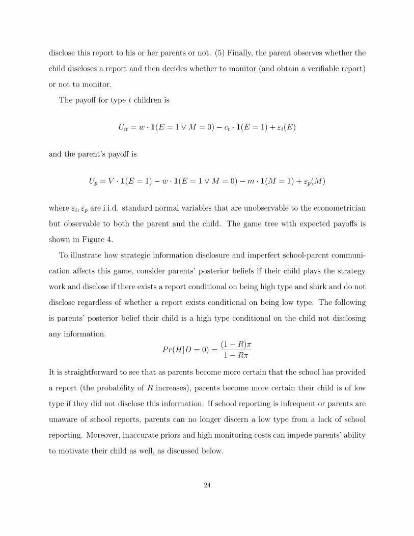
The payoff for type t children is

Uit = w · 1(E = 1 ∨M = 0)− ct · 1(E = 1) + εi(E)

and the parent’s payoff is

Up = V · 1(E = 1)− w · 1(E = 1 ∨M = 0)−m · 1(M = 1) + εp(M)

where εi, εp are i.i.d. standard normal variables that are unobservable to the econometrician

but observable to both the parent and the child. The game tree with expected payoffs is

shown in Figure 4.

To illustrate how strategic information disclosure and imperfect school-parent communi-

cation affects this game, consider parents’ posterior beliefs if their child plays the strategy

work and disclose if there exists a report conditional on being high type and shirk and do not

disclose regardless of whether a report exists conditional on being low type. The following

is parents’ posterior belief their child is a high type conditional on the child not disclosing

any information.

Pr(H|D = 0) =(1−R)π

1−Rπ

It is straightforward to see that as parents become more certain that the school has provided

a report (the probability of R increases), parents become more certain their child is of low

type if they did not disclose this information. If school reporting is infrequent or parents are

unaware of school reports, parents can no longer discern a low type from a lack of school

reporting. Moreover, inaccurate priors and high monitoring costs can impede parents’ ability

to motivate their child as well, as discussed below.

24

Identification

Many issues arise in estimation due to the fact that, for a given set of ε, there are multiple

possible equilibria. Much of the literature on the estimation of static games deals with the

issue of multiple equilibria (Bresnahan and Reiss 1990; Bresnahan and Reiss, 1991; Berry,

1992; Bajari, Hong, and Ryan, 2010). Kim (2015) uses equilibrium refinement of Cho and

Kreps (1987) to eliminate multiple equilibria in the context of a two-player signaling game.

I enumerate conditions below to refine the set of equilibria.

The game is characterized by seven structural objects and I impose the following identi-

fying restrictions:

1. cL > 0: cost of effort for L-types.

2. cH < cL: cost of effort for H-types.

3. m > 0: the monitoring cost for the parent.

4. 0 < R < 1: the probability of a report being generated.28

5. 0 < π < 1: the distribution of types.

6. V > 0: the utility to parents from their child’s effort.

7. w > 0: the reward from parents to their child for their effort.

Under these conditions there is a mapping of preferences and parameters to unique, Perfect

Bayesian Equilibria. Figure 5 summarizes this mapping. All Perfect Bayesian Equilibria—

separating, pooling and hybrid—are derived in the appendix.

Estimation

With the uniqueness of the equilibria under the above conditions, I estimate the model us-

ing maximum likelihood. I construct the likelihood function as follows. First, I define the

28This restriction implies all beliefs are on the equilibrium path.

25

probability for each set of actions, a = (M,E,D) and equilibrium. To derive these proba-

bilities, I multiply the probability of an action given the parameters θ and the equilibrium

that occurs, P (a|Eq, θ), by the probability that the equilibrium occurs, P (Eq). For example,

the probability of a = (1, 1, 1) given the first separating equilibrium in the appendix, S1, is

the probability that a high type is drawn and a report is generated. The probability that

equilibrium S1 is drawn is (Φ(w − cH) − Φ(w − cL))Φ(−m) where Φ(·) is the cumulative

normal distribution function. Constructing the joint probabilities with hybrid equilibria is

slightly more involved and evaluated for a given set of parameters using standard Monte

Carlo integration. All derivations are detailed in the appendix.

The probability of observing each event a is the sum of the joint probabilities of a and

equilibria eq.

P (a|θ) =∑eq∈Eq

P (a, eq|θ)

To set up the likelihood function, let j be the observation of parent-child pairs with parent

actions indexed by p and child actions index by i. The observed actions are: mpj, eij, dij for

monitoring, effort and disclosure, respectively, for observation j. The likelihood function is

logL((mp, ei, di)|θ) =1

n

n∑j=1

(mpjeijdij logP ((1, 1, 1)|θ) +mpjeij(1− dij) logP ((1, 1, 0)|θ)

+mpj(1− eij)(1− dij) logP ((1, 0, 0)|θ)

+ (1−mpj)eijdij logP ((0, 1, 1)|θ)

+ (1−mpj)eij(1− dij) logP ((0, 1, 0)|θ)

+ (1−mpj)(1− eij)(1− dij)P ((0, 0, 0)|θ)

Given the payoff structure, the difference between V and w is not identified. I normalize

the former to one. In addition to the parameter estimates, I also present the estimated dis-

tribution of equilibria in the results below. I estimate the model separately for the treatment

26

and control groups.

Measures, Estimates, and Simulations

I use survey measures of punishment and disclosure described previously to generate indica-

tors for whether the child was punished due to their schoolwork or grades and whether the

child informs his or her parents about their academic progress, respectively. An indicator

for effort is constructed in line with the report-card measure of effort studied previously; any

unsatisfactory effort is assigned a zero and is a one otherwise. Despite summarizing these

measures into unidimensional, binary variables, they follow the equilibrium predictions of

the model well. For instance, all but one child who exerts effort also discloses to parents,

and children who exert effort are rarely punished by parents (6 students).29

Note that not all families arrive at the same equilibrium. Heterogeneity stems from

differences in parental beliefs between the treatment and control groups and the idiosyncratic

component of families’ utility functions. Table A.10 shows this point by presenting the

distribution of equilibria for the treatment and control group, respectively. The proportions

of certain separating equilibria, in particular, change across the two groups; the treatment

shifts families toward separating and pooling equilibria with greater monitoring.

Table 12 presents the key parameter estimates, which show the intervention operates

through a combination of effects. Compared to the treatment group, parents in the control

group experience higher monitoring costs (higher M), are less likely to believe they can track

their child’s effort (lower R), and are significantly more likely to believe their child is a high

type (higher π). As expected, these results are in line with the reduced-form findings, which

shows revisions of parental beliefs and higher rates of contact with the school to discuss

their child’s academic progress. To understand whether the magnitudes of these estimates

are reasonable, and how well the model fits the data, in the online appendix I show how

well the simulated moments match their observed observed. The model matches observed29These observations are dropped from the estimation.

27

measures of effort and disclosure well in both groups, though it slightly underestimates

monitoring rates in the treatment group (Table A.11).

With these parameter estimates, I can also decompose the treatment effects on children’s

effort. The empirical treatment effect on the measure of effort is 4.2 percentage points, which

is closely replicated by the model at 4.37 percentage points. The latter replication is not

entirely surprising given that the model is estimated separately for the treatment and control

group. However, I can vary certain parameters while holding others constant. Monitoring

costs also explain a substantial portion of the effects, 54%. Equating the control group’s

beliefs to the treatment group’s beliefs accounts for 42% of the treatment effect. The change

in reporting accounts for only 3%. The substantial contribution to changes in beliefs could

partly explain the persistence of the impacts into the following semester.

Moreover, these results suggest another simple policy tool schools can use to improve

outcomes: improving school reporting. School districts vary in how often teachers must

grade materials and enter them into a gradebook. While some parents face low monitoring

costs and can find time to speak directly with teachers, low-income families are more likely

single-parent households facing changing work schedules and transportation problems that

make monitoring more difficult (Lott, 2001). Improved school reporting allows parents to

more effectively target their monitoring. I simulate a policy that increases the likelihood of

a report to 85% and, implicitly, makes this change salient to families. Increasing reporting

in this way would cause an increase in effort by 2.15 percentage points for the control group,

or roughly half the effect of providing additional information to families. While smaller in

magnitude, this policy may be less controversial and easier to implement than output-focused

policies, such as incentivizing teachers’ value added.

28

VII Conclusion and Cost effectiveness

This paper uses an experiment to answer how information asymmetries between parents and

their children affect human capital investment and achievement. The results show these

problems can be significant and their effect on achievement large. Additional information

to parents about their child’s missing assignments and grades helps parents motivate their

children more effectively and changes parents’ beliefs about their child’s effort in school.

Parents also become more aware that their child does not tell them enough about their

academic progress. These mechanisms drive an almost .20 standard deviation improvement

in math standardized test scores and GPA. There is no estimated effect on middle-school

family outcomes, however there was severe contamination in the middle school sample. One

positive aspect of this contamination is that it reflects teachers’ valuation of the intervention,

which has helped scale this work further.

However it is important to consider how well these results extrapolate to other contexts.

Identifying the mechanisms driving the treatment effects provides insight into the external

validity of the findings. For instance, there is evidence that the information problems encoun-

tered in the context of this paper are more widespread. First, several papers document that

parents in low-performing schools have upwardly biased beliefs about their child’s academic

performance both in the United States context (Bonilla et al., 2005; Kinsler and Pavan,

2016) and outside the United States (Dizon-Ross, 2016). Second, there is also evidence from

the United States that the quality of school reporting is poor: in schools where the majority

of students do not go on to college, only 43% of parents are satisfied with the communication

they receive from their child’s school about their schoolwork and grades (Bridgeland et al.,

2008).

A limitation of this study is that the treatment lasted six months. The negative informa-

tion about academic performance could create tension at home that might impact outcomes

differently over the long run, which makes direct comparison to other, longer-run interven-

29

tions difficult. However parents expressed a desire to continue the information service and

treatment effects persisted into the following academic year, after the intervention concluded.

Importantly, this paper demonstrates several potentially cost-effective ways to bolster

student achievement. For instance, contacting parents via text message, phone call or email

took approximately three minutes per student. Gathering and maintaining contact numbers

adds five minutes of time per child, on average. The time to generate a missing-work report

can be almost instantaneous or take several minutes depending on the grade book used

and the coordination across teachers.30 For this experiment it was roughly five minutes.

Teacher overtime pay varies across districts and teacher characteristics, but a reasonable

estimate prices their time at $40 per hour. If teachers were paid to coordinate and provide

information, the total cost per child per .10 standard-deviation increase in GPA or math

scores would be $156.31

Automating aspects of this process could reduce this costs further, especially because

many districts pay fixed costs for data systems. In response to this experiment, the school

and a learning management company collaborated to develop a feature that automatically

text messages parents about their child’s missing assignments directly from teachers’ grade

books, which has been scaled to a large district. Relative to other effective interventions

targeting adolescent achievement, the additional marginal cost is quite low.

30Some grade book programs can produce a missing assignment report for all of a student’s classes.31This cost-effectiveness analysis excludes the potentially significant time costs to parents and children.

30

References

[1] Aaronson, Daniel, Lisa Barrow and William Sander (2007). “Teachers and Student

Achievement in the Chicago Public High Schools,” Journal of Labor Economics, vol

25(1), 95-135.

[2] Abdulkadiroglu, Atila, Joshua D. Angrist, Susan M. Dynarski, Thomas J. Kane and

Parag A. Pathak (2011). “Accountability and Flexibility in Public Schools: Evidence

from Boston’s Charters and Pilots,” The Quarterly Journal of Economics, 126, 699-748.

[3] Akabayashi, Hideo (2006). “An Equilibrium Model of Child Maltreatment,” Journal of

Economic Dynamics & Control 30(6): 993-1025.

[4] Andrabi, Tahir, Jishnu Das and Asim Ijaz Khwaja (2009). “Report Cards: The Impact

of Providing School and Child Test-Scores on Educational Markets,” Mimeo, Harvard

University.

[5] Angrist, Joshua D., Susan M. Dynarski, Thomas J. Kane, Parag A. Pathak, Christopher

R. Walters (2010). “Inputs and Impacts in Charter Schools: KIPP Lynn,” American

Economic Review: Papers and Proceedings, vol 100(2), 239-243.

[6] Angrist, Joshua D. and Victor Lavy (2002). “The Effects of High Stakes High School

Achievement Awards: Evidence from a Randomized Trial,” American Economic Review,

vol 99(4), 1384-1414.

[7] Avvisati, Francesco, Marc Gurgand, Nina Guyon and Eric Maurin (2013). “Getting Par-

ents Involved: A Field Experiment in Deprived Schools,” Review of Economic Studies,

vol 81(1): 57-83.

[8] Bajari, Patrick, Han Hong, and Stephen Ryan (2010). “Identification and Estimation of

a Discrete Game of Complete Information,” Econometrica, vol 78(5): 15291568.

31

[9] Berry, James (2011). “Child Control in Education Decisions: An Evaluation of Targeted

Incentives to Learn in India,” Mimeo, Cornell University.

[10] Berry, Steven (1992). “Estimation of a Model of Entry in the Airline Industry,” Econo-

metrica, vol 60(4): 889-917.

[11] Bettinger, Eric P. (2010). “Paying to Learn: The Effect of Financial Incentives on

Elementary School Test Scores,” NBER Working Paper No. 16333.

[12] Bettinger, Eric, Bridget T. Long, Philip Oreopoulos and Lisa Sanbonmatsu (2009). “The

Role of Simplification and Information in College Decisions: Results from the H&R Block

FAFSA Experiment,” NBER Working Paper No. 15361.

[13] Bettinger, Eric and Robert Slonim (2007). “Patience in Children: Evidence from Ex-

perimental Economics,” Journal of Public Economics, vol 91(1-2): 343-363.

[14] Bonilla, Sheila, Sara Kehl, Kenny Kwong, Tricia Morphew, Rital Kachru and Craig

Jones (2005). “School Absenteeism in Children With Asthma in a Los Angeles Inner

City School,” The Journal of Pediatrics 147(6): 802-806.

[15] Bresnahan, Timothy and Peter Reiss (1990). “Entry in Monopoly Markets,” The Review

of Economic Studies 57(4): 531-553.

[16] Bresnahan, Timothy and Peter Reiss (1991). “Entry and Competition in Concentrated

Markets,” The Journal of Political Economy 99(5): 977-1005.

[17] Bridgeland, John M., John J. Dilulio, Ryan T. Streeter, and James R. Mason (2008).

One Dream, Two Realities: Perspectives of Parents on America’s High Schools, Civic

Enterprises and Peter D. Hart Research Associates.

[18] Buddin, Richard (2010). “How Effective Are Los Angeles Elemen-

tary Teachers and Schools?” Retrieved online on April 2011, from

32

http://s3.documentcloud.org/documents/19505/how-effective-are-los-angeles-

elementary-teachers-and-schools.pdf.

[19] Bursztyn, Leonardo and Lucas Coffman (2012). “The Schooling Decision: Family Pref-

erences, Intergenerational Conflict, and Moral Hazard in the Brazilian Favelas,” Journal

of Political Economy, vol 120(3): 359-397 .

[20] Cameron, Colin, Jonah Gelbach and Douglas Miller (2008). “Bootstrap-Based Improve-

ments for Inference with Clustered Standard Errors,” The Review of Economics and

Statistics, vol 90(3): 414-427.

[21] Cosconati, Marco (2009). “Parenting Style and the Development of Human Capital in

Children,” Ph.D. dissertation, University of Pennsylvania.

[22] Cunha, Flavio, Irma Elo and Jennifer Culhane (2013). “Eliciting Maternal Expectations

about the Technology of Cognitive Skill Formation,” NBER Working Paper No. 19144.

[23] Cunha, Flavio and James J. Heckman (2007), “The Technology of Skill Formation,”

The American Economic Review, vol 97: 31-47.

[24] Cunha, Flavio, James J. Heckman, Lance Lochner and Dimitriy V. Masterov (2006),

“Chapter 12 Interpreting the Evidence on Life Cycle Skill Formation,” Handbook of the

Economics of Education, vol 1: 697-812.

[25] Dizon-Ross, Rebecca (2016), “Parents’ Beliefs and CHildren’s Education: Experimental

Evidence from Malwai,” Working paper.

[26] Dobbie, Will and Roland G. Fryer (2011). “Are High Quality Schools Enough to Close

the Achievement Gap? Evidence from the Harlem Children’s Zone,” American Journal:

Applied Economics, vol 3(3), 158-187.

[27] Dudovitz, Rebecca, Ning Li and Paul Chung (2013). “Behavioral Self-Concept as Pre-

dictor of Teen Drinking Behaviors,” Academic Pediatrics 13(4): 316-321.

33

[28] Dye, Ronald (1985). “Disclosure of Nonproprietary Information,” Journal of Accounting

Research 23(1): 123-145.

[29] French, Michael, Jenny Homer and Philip K. Robins (2010). “What You Do in High

School Matters: The Effects of High School GPA on Educational Attainment and Labor

Market Earnings in Adulthood.” Mimeo, University of Miami, Department of Economics.

[30] Fryer, Roland G. (2010). “Financial Incentives and Student Achievement: Evidence

from Randomized Trials,” NBER Working Paper No. 15898.

[31] Fryer, Roland G. (2011). “Teacher Incentives and Student Achievement: Evidence from

New York City Public Schools,” NBER Working Paper No. 16850.

[32] Gelser, Saul and Marla V. Santelices (2007). “Validity of High-School Grades in Predict-

ing Student Success Beyond the Freshman Year: High-School Record vs. Standardized

Tests as Indicators of Four-Year College Outcomes,” Research & Occasional Paper Series:

CSHE.6.07.

[33] Green, Leonard, Astrid Fry and Joel Myerson (1994). “Discounting of Delayed Rewards:

A Life-Span Comparison,” Psychological Science 5(1): 33-36.

[34] Grossman, Sanford (1981). “The Informational Role of Warranties and Private Disclo-

sure about Product Quality,” Journal of Law and Economics 24(3): 461-483.

[35] Hao, Lingxin, V. Joseph Hotz and Ginger Zin (2008). “Games Parents and Adolescents

Play: Risky Behaviour, Parental Reputation and Strategic Transfers,” The Economic

Journal 118(528): 515-555.

[36] Hastings, Justine S. and Jeffrey M. Weinstein (2008). “Information, School Choice, and

Academic Achievement: Evidence from two Experiments” Quarterly Journal of Eco-

nomics, vol 123(4) 1373-1414.

34

[37] Heckman, James J. and Stefano Mosso (2014). “The Economics of Human Development

and Social Mobility,” Annual Review of Economics Vol. 6: 689-733.

Heckman, James, Seong Hyeok Moon, Rodrigo Pinto, Peter Savelyev and Adam Yavitz

(2010). “Analyzing social experiments as implemented: A reexamination of the evidence

from the HighScope Perry Preschool Program, Quantitative Economics 1(1): 1-46.

[38] Heckman, James J. and Rodrigo Pinto (2013). “Econometric Mediation Analyses: Iden-

tifying the Sources of Treatment Effects from Experimentally Estimated Production Tech-

nologies with Unmeasured and Mismeasured Inputs,” NBER Working Paper No. 19314.

[39] Heckman, James, Rodrigo Pinto and Peter Savelyev (2013). “Understanding the Mech-

anisms Through Which an Influential Early Childhood Program Boosted Adult Out-

comes,” American Economic Review 103(6): 2052-2086.

[40] Houtenville, Andrew J. and Karen Smith Conway (2008), “Parental Effort, School Re-

sources and Student Achievement,” Journal of Human Resources, vol 43(2): 437-453.

[41] Imai, Kosuke, Dusting Tingley and Luke Keele (2010). “A General Approach to Causal

Mediation Analysis,” Psychological Methods 15(4): 309-334.

[42] Jacob, Brian and Lars Lefgren (2008). “Can Principals identify Effective Teachers? Evi-

dence on Subjective Performance Evaluation in Education,” Journal of Labor Economics,

vol 26(1), 101-136.

[43] Kim, Kyoo il (2015). “Semiparametric Estimation of Signaling Games with Equilibrium

Renement ,” Michigan State University Working Paper.

[44] Kinsler, Josh and Ronni Pavan (2016), “Parental Beliefs and Investment in Children,”

Working paper.

35

[45] Levitt, Steven D., John A. List, Susanne Neckermann and Sally Sadoff (2011). “The

Impact of Short-Term Incentives on Student Perofrmance” Mimeo, University of Chicago,

Becker Friedman Institute.

[46] Los Angeles Unified School District (2009). “Memorandum of Un-

derstanding Between Los Angeles Unified School District and United

Teachers Los Angeles.” Retrieved on January 10, 2011, from

http://publicschoolchoice.lausd.net/sites/default/files/Los%20Angeles%20Pilot%

20Schools%20Agreement%20%28Signed%29.pdf.

[47] Los Angeles Unified School District (2011). School Report Cards. Retrieved on January

10, 2011, from http://getreportcard.lausd.net/reportcards/reports.jsp.

[48] Lott, B. (2001). “Low-income parents and the public schools,” Journal of Social Issues,

57(2): 247259.

[49] Milgrom, Paul (1981). “Good News and Bad News: Representation Theorems and Ap-

plications,” The Bell Journal of Economics 12(2): 380-391.

[50] Miller, Cynthia, James Riccio and Jared Smith (2009). “A Preliminary Look at Early

Educational Results of the Opportunity NYC-Family Rewards Program” MDRC.

[51] Rivkin, Steven G., Eric A. Hanushek and John F. Kain (2005). “Teachers, Schools, and

Academic Achievement,” Econometrica, vol 73(2), 417-458.

[52] Rockoff, Jonah E., Douglas O. Staiger, Thomas J. Kane and Eric S. Taylor (2010).

“Information and Employee Evaluation: Evidence from a Randomized Intervention in

Public Schools,” NBER Working Paper No. 16240.

[53] Romano, Joseph and Michael Wolf (2005). “Exact and Approximate Stepdown Meth-

ods for Multiple Hypothesis Testing, Journal of the American Statistical Association

100(469): 94-108.

36

[54] Romano, Joseph and Michael Wolf (2005). “Stepwise Multiple Testing as Formalized

Data Snooping, Econometrica 73(4): 1237-1282.

[55] Romano, Joseph, Azeem Shaikh and Michael Wolf (2010). ‘Hypothesis Testing in Econo-

metrics, Annual Review of Economics 2: 75-104.

[56] Rosenbaum, James E. (1998). “College-for-All: Do Students Understand What College

Demands?” Social Pyschology of Education, vol 2(1) 55-80.

[57] SFGate.com (2010). Poll Finds Most Blame Parents for School Woes. Retrieved on

January 10, 2011, from http://articles.sfgate.com/2010-12-12/news/25188015 1 parents-

united-responsible-education-student-discipline.

[58] Shin, Hyun Song (1994). “The Burden of Proof in a Game of Persuasion,” Journal of

Economic Theory 64(1): 253-264.

[59] Springer, Matthew G., D. Ballou, L. Hamilton, V. Le, J.R. Lockwood, D. McCaffrey,

M. Pepper and B. Stecher (2010). “Teacher Pay for Performance: Experimental Evi-

dence from the Project on Incentives in Teacher,” Nashville, TN: National Center on

Performance Incentives at Vanderbilt University.

[60] Stattin, Hakan and Margaret Kerr (2000). “Parental Monitoring: A Reinterpretation,”

Child Development, vol 71(4), 1072-1085.

[61] Steinberg, Laurence, Lia O’Brien, Elizabeth Cauffman, Sandra Graham, Jennifer

Woolard and Marie Banich (2009). “Age Differences in Future Orientation and Delay

Discounting” Child Development, vol 80(1): 28-44.

[62] Time Magazine (2010). TIME Poll Results: Americans’ Views on Teacher Tenure,

Merit Pay and Other Education Reforms. Retrieved online on January 10, 2011, from

http://www.time.com/time/nation/article/0,8599,2016994,00.html#ixzz1dFb1oSwE.

37

[63] Todd, Petra and Kenneth I. Wolpin (2007), “The Production of Cognitive Achievement

in Children: Home, School and Racial Test Score Gaps,” Journal of Human Capital, vol

1(1): 91-136.

[64] Valeri, Linda and Tyler VanderWeele (2013). “Mediation Analysis Allowing for

Exposure-Mediator Interactions and Causal Interpretation: Theoretical Assumptions and

Implementation With SAS and SPSS Macros” Psychological Methods 18(2): 137-150.

[65] Weinberg, Bruce (2001), “An Incentive Model of the Effect of Parental Income on Chil-

dren,” Journal of Political Economy, vol 109(2): 266-280.

38

Figure 1: Timeline

This figure shows the timeline of the experiment. Above the timeline is a chart of the frequency ofmessages sent to parents. Each bar signifies the number of messages sent over a three-day period andcorresponds to the timeline dates below. The abbreviations HS and MS indicate that messages weresent to families of high school (HS) students families on alternate weeks with respect to middle school(MS) students families. “Std. tests” shows when the state-mandated standardized tests took place.

39

Figure 2: Parental Beliefs Relative to Truth

This figure shows a kernel-density plot of the true number of math assignmentsmissed by a student minus the number of missed assignments estimated by parentsvia survey. Data come from surveys of parents and teacher grade books.

Figure 3: GPA over time for high school students

1.95

2

2.05

2.1

2.15

2.2

2.25

2.3

GP

A

01no

v201

0

01de

c201

0

01jan

2011

01fe

b201

1

01m

ar20

11

01ap

r201

1

01m

ay20

11

01jun

2011

01jul

2011

Date

treatment group control group

This graph plots the GPA of high school students in the treatment and control groupover time. Each point represents the average GPA in a group calculated from progressreport grades. The vertical red line indicates when the treatment began. To hold thecomposition of the sample constant over time, this plot excludes students who left theschool prior to the end of the second semester.

40

NS

P

M = 1M = 0

E = 1, D = 1

P

M = 0 M = 1

E = 0, D = 0

πS

P

M = 1M = 0

E = 1, D = 1

P

M = 0 M = 1

E = 0, D = 0

1− π

(w − cH , V − w −m)(w − cH , V − w) (w − cL, V − w −m)(w − cL, V − w)

(w,−w) (0,−m) (w,−w) (0,−m)

Figure 4: figureGame Tree

This figure presents the persuasion game between parents and their children. Nature (N) selects the child’s type withprobability π. The student (S) then decides to exert effort (E) and disclose their progress (D) or to not exert effort andnot disclose. Parents (P) then decide to monitor (M) their child or not and reward them (w) accordingly. The cost ofeffort is cH and cL for a high type and low type of student, respectively. Parents value their child’s effort at V and pay acost of monitoring of m.

41

−m

−m+ 1−π1−Rπw

−m+ w

−cL −cH w − cL w − cH

εi(0)− εi(1)

ε p(0

)−ε p

(1)

S1

S2

S3

P1

P2 P3

P4

P5

H1

H2

Figure 5: Equilibria of Game

This figure presents the mapping from the parameters of the model to the specific equilibria. S1-S3 index separating equlib-ria, P1-P5 index pooling equilibria, and H1 and H2 index hybrid equilibria. Further information about each equilibriumand its derivation is in the appendix.

42

Table 1: Correlations with Parental Beliefs of Student Effort

(1) (2) (3) (4)Dependent variable GPA GPA GPA GPA

Difference from Truth -0.040***(0.007)

Contacted School -0.031*(0.016)

Privileges -0.091***(0.019)

Kid does not Disclose -0.697***(0.143)

Observations 149 255 256 250R-squared 0.366 0.013 0.122 0.086

This table shows associations between parent survey items and student performance.Column (1) shows the correlation of the true number of math assignments missed bya student minus the number of missed assignments estimated by parents with GPA.Sample size varies by response rate. Robust standard errors are in parentheses.

*** p<0.01, ** p<0.05, * p<0.1

43

Table 2: Summary Statistics and Treatment-Control Group Balance

Panel A. Sample balance including attriters

Control Mean Treatment Mean Difference P-value Students Obs.

Female 0.363 0.463 0.099 0.078 306 306Attendance 0.928 0.942 0.014 0.278 306 306Baseline GPA 2.019 1.995 -0.024 0.848 298 298Prior GPA 2.173 2.043 -0.130 0.282 252 252Asian 0.24 0.219 -0.021 0.664 306 306Black 0.021 0.031 0.011 0.559 306 206Hispanic 0.699 0.725 0.026 0.612 306 306Parent graduated HS 0.205 0.231 0.026 0.588 306 306Free/Reduced Lunch 0.89 0.869 -0.022 0.563 306 306Work habits unsatisfactory 0.326 0.308 -0.019 0.585 297 1953Cooperation unsatisfactory 0.111 0.105 0.006 0.751 297 1952Work habits excellent 0.354 0.310 -0.044 0.207 297 1953Cooperation excellent 0.487 0.458 -0.029 0.385 297 1952

Panel B. Sample balance excluding attriters

Control Mean Treatment Mean Difference P-value Students Obs.

Female 0.382 0.462 0.079 0.182 279 279Attendance 0.949 0.952 0.003 0.797 279 279Baseline GPA 2.124 2.068 -0.056 0.658 272 279Prior GPA 2.267 2.137 -0.130 0.289 228 228Asian 0.243 0.238 -0.005 0.924 279 279Black 0.022 0.028 0.006 0.753 279 279Hispanic 0.691 0.706 0.015 0.784 279 279Parent graduated HS 0.213 0.238 0.025 0.626 279 279Free/Reduced lunch 0.904 0.888 -0.016 0.657 279 279Work habits unsatisfactory 0.298 0.291 -0.007 0.846 279 1804Work habits excellent 0.374 0.326 -0.048 0.188 279 1804Cooperation unsatisfactory 0.089 0.093 0.003 0.855 279 1803Cooperation excellent 0.511 0.482 -0.029 0.388 279 1803

Note: p-values are for tests of equality of means across the treatment and control group. Differences across work habits and cooperationare estimated by a regression of the behavior on treatment status with standard errors clustered by student. Baseline data are missingfor students who enrolled in the school after the school year began. The “Students” column reports the number of student-levelobservations used in the analysis. The “Obs.” column shows the total number of observations. The number of observations differs fromthe number of students for work habits and cooperation because a student receives these marks for each class he or she takes.

44

Table 3: Contact from the School Regarding Grades

(1) (2)

Dependent variable

Schoolcontactto parent

Contactedmorethan once

Treatment 2.125*** 0.453***(0.370) (0.068)

Baseline GPA 0.100 -0.105**(0.411) (0.052)

Prior GPA -0.125 0.100*(0.341) (0.051)

Control mean 1.134 0.286

Observations 183 183R-squared 0.173 0.248

The dependent variable is drawn from surveys of par-ents. Parents were asked how many times they werecontacted by the school regarding their child’s grades orschoolwork during the last month of school. Column (1)uses the number of times contacted by the school as thedependent variable while column (2) uses an indicatorfor whether a parent was contacted more than one time.Baseline GPA is calculated from students’ mid-semesterprogress reports from two months before the experimentbegan. Prior GPA is students’ cumulative GPA frommiddle school and beyond. Strata and grade-level indica-tors are also included in each regression. Robust standarderrors are in parentheses.

*** p<0.01, ** p<0.05, * p<0.1

45

Table 4: GPA effect on High School Students

(1) (2) (3)Dependent variable GPA GPA GPA

Treatment 0.145 0.203** 0.229**(0.143) (0.093) (0.090)

Baseline GPA 0.931*** 0.760***(0.060) (0.071)

Prior GPA 0.334***(0.072)

Grade 10 -0.248**(0.119)

Grade 11 -0.164(0.117)

Observations 279 279 279R-squared 0.004 0.601 0.645

The dependent variable is students’ end-of-semester GPA. Data used in theseregressions are from administrative records. Baseline GPA is calculated fromstudents’ mid-semester progress reports from two months before the treat-ment began. Prior GPA is students’ cumulative GPA from middle schooland beyond. Strata indicators are also included in each regression. Highschool in this sample includes only grades nine through eleven because theschool had just opened. Robust standard errors are in parentheses.

*** p<0.01, ** p<0.05, * p<0.1

Table 5: Effects on Grades

(1) (2) (3) (4)Dependent variable Class Grade Class Grade Class Grade Class Grade

Treatment 0.231*** 0.188** 0.208** 0.232**(0.088) (0.095) (0.089) (0.090)

Treatment*Target 0.120(0.086)

Treatment*Math class 0.212(0.132)

Treatment*English class 0.022(0.119)

Students 279 279 279 279Observations 2,224 2,224 2,224 2,224R-squared 0.399 0.438 0.417 0.405

The dependent variable in these regressions is each students’ class grade, which is coded into a four-pointscale from their letter grades. Data used in these regressions are from administrative records. Each studenttypically takes eight classes. Grades marked incomplete are coded as missing. Additional controls in eachregression are students’ baseline GPA, prior GPA, grade-level indicators and strata indicators. BaselineGPA is calculated from students’ mid-semester progress reports from two months before the treatmentbegan. Prior GPA is students’ cumulative GPA from middle school and beyond. Standard errors clusteredby student are in parentheses.

*** p<0.01, ** p<0.05, * p<0.1

46

Table 6: Effects on Final Exams and Projects

(1) (2) (3) (4)Dependent variable: All Scores Math Scores English Scores No Score

Treatment 0.160** 0.180* 0.329** -0.075***(0.081) (0.110) (0.106) (0.034)

Students 279 239 100 279Observations 639 239 100 676R-squared 0.347 0.430 0.465 0.184

All exam and final project scores are standardized by class to have a mean equal to zero anda standard deviation equal to one. Data in these regressions are from teacher grade books.Additional controls not shown are baseline GPA, prior GPA, grade-level indicators and strataindicators. Baseline GPA is calculated from students’ mid-semester progress reports from twomonths before the experiment began. Prior GPA is students’ cumulative GPA from middle schooland beyond. The final column shows the effect of the treatment on not having score, excludingexcused absences. If a student does not have a score it means they did not turn in any test orproject. 18% of tests or final projects were not turned in by the control group. Standard errorsclustered by student are in parentheses.

*** p<0.01, ** p<0.05, * p<0.1

47

Tab

le7:

Eff

ects

on

Sta

nd

ard

ized

Tes

tS

core

s

(1)

(2)

(3)

(4)

(5)

(6)

Dep

end

ent

vari

able

Mat

hS

core

Math

Sco

reM

ath

Sco

reE

ngli

shS

core

En

gli

shS

core

En

gli

shS

core

Tre

atm

ent

0.07

70.2

12**

-0.1

84

-0.0

39

0.0

08

0.0

36

(0.1

07)

(0.1

02)

(0.2

36)

(0.2

26)

(0.0

91)

(0.2

09)

Bas

elin

eG

PA

0.31

1***

0.2

45**

0.1

19

0.5

39***

0.3

39***

0.3

46***

(0.0

76)

(0.0

91)

(0.1

04)

(0.0

83)

(0.0

78)

(0.1

01)

Pri

orG

PA

0.29

2***

0.2

59***

0.1

98***

0.1

40*

0.0

75

0.0

18

(0.0

84)

(0.0

77)

(0.0

81)

(0.0

78)

(0.0

70)

(0.0

71)

Tre

atm

ent*

bas

elin

eG

PA

0.1

92**

-0.0

13

(0.1

01)

(0.0

90)

Ad

dit

ion

alco

ntr

ols

No

Yes

Yes

No

Yes

Yes

Ob

serv

atio

ns

256

256

256

257

257

257

R-s

qu

ared

0.30

60.4

57

0.4

68

0.3

37

0.6

05

0.6

05

This

table

rep

ort

sth

eeff

ect

of

the

treatm

ent

on

the

state

-mandate

dte

st,

the

Califo

rnia

Sta

ndard

sT

est

,fo

rhig

hsc

hool

students

.Score

sare

standard

ized

by

test

sub

ject

tohave

am

ean

of

zero

and

ast

andard

devia

tion

equal

toone.

The

addit

ional

contr

ols

not

show

nab

ove

are

pri

or

test

score

s,ra

ce,

sex,

test

sub

ject,

language

spoken

at

hom

eand

free

or

reduced-p

rice

lunch

statu

s.B

ase

line

GP

Ais

GP

Acalc

ula

ted

from

students

’m

id-s

em

est

er

pro

gre

ssre

port

stw

om

onth

sb

efo

reth

etr

eatm

ent

began.

Pri

or

GP

Ais

students

’cum

ula

tive

GP

Afr

om

mid

dle

school

and

beyond.

Robust

standard

err

ors

are

inpare

nth

ese

s.

***

p<

0.0

1,

**

p<

0.0

5,

*p<

0.1

48

Table 8: Impact of Information on Parental Beliefs

Panel A. Effect on Parental Beliefs

Dependent variable Pr(Don’t Know) Pr(missed 0-2) Pr(missed 3-5) Pr(missed 5+)

Treatment -0.130** -0.028 0.160** -0.002(0.062) (0.070) (0.066) (0.045)

Observations 172 172 172 172

Panel B. Effect on Accuracy of Beliefs

Dependent variableDifferencefrom Truth

Differencefrom Truth

KidDoesn’tDisclose

Treatment -5.564* -15.541** 0.195***(3.022) (7.283) (0.070)

Treatment*Baseline GPA 4.606*(2.421)

Control Mean 14.337 0.210

Observations 91 91 176R-squared 0.485 0.512 0.160

This table shows the impact of the treatment on parental beliefs about the number of missed assignments their child has missedin math class. Results in Panel A show average marginal effects. Panel A includes parents who respond “I don’t know” whilePanel B excludes these respondents. Data comes from surveys of parents of high school students. Difference from truth outcomehas fewer observations because this measure requires observed assignment information and a parent-survey response. Robuststandard errors are in parentheses.

*** p<0.01, ** p<0.05, * p<0.1

49

Table 9: Parents’ Responses to Additional Information

Panel A. Parental Monitoring

Dependent variableContactedSchool

AttendedConference Ask HW

Treatment 1.783*** 0.079* -2.533(0.668) (0.046) (1.688)

Control Mean 2.102 0.150 18.773

Data source Parent School ParentObservations 179 181 184R-squared 0.147 0.105 0.048

Panel B. Parental Incentives and Assistance

PrivilegesDependent variable Taken Talk College Help Child Can Help

Treatment 1.660** 2.611* 0.088 0.161**(0.718) (1.415) (0.069) (0.072)

Control Mean 1.729 7.637 0.210 0.600

Data source Parent Parent Child ParentObservations 180 183 183 181R-squared 0.168 0.163 0.091 0.101

All columns show the effects of the information treatment on parents. Treatment effects areestimated using regressions that control for baseline GPA, prior GPA, strata indicators and grade-level indicators. Baseline GPA is GPA calculated from students’ mid-semester progress reports twomonths before the experiment began. Prior GPA is students’ cumulative GPA from middle schooland beyond. Data source indicates whether the dependent variable came from a parent’s surveyresponse, a child’s survey response, or school records. Robust standard errors are in parentheses.

*** p<0.01, ** p<0.05, * p<0.1

50

Tab

le10:

Eff

ects

on

Beh

avio

rs

In-C

lass

Work

Hab

its

In-C

lass

Coop

era

tion

Dep

end

ent

vari

able

Pr(

Un

sati

sfact

ory

)P

r(E

xce

llen

t)P

r(U

nsa

tisf

act

ory

)P

r(E

xce

llen

t)

Tre

atm

ent

-0.0

61***

0.0

69***

-0.0

24**

0.0

56**

(0.0

21)

(0.0

22)

(0.0

11)

(0.0

24)

Pre

dic

ted

pro

bab

ilit

y0.

256

0.3

39

0.0

96

0.4

32

Stu

den

ts27

9279

279

279

Ob

serv

atio

ns

8,795

8,7

95

8,7

95

8,7

95

Att

en

dan

ce

Ass

ign

ment

Com

ple

tion

Dep

end

ent

Var

iab

le:

Fu

ll-d

ayR

ate

By-C

lass

Rate

Cla

sses

Mis

sed

Pr(

Mis

sed

Ass

t.)

Tre

atm

ent

1.67

52.8

79*

-1.4

01**

-0.0

49***

(1.1

46)

(1.5

40)

(0.6

33)

(0.0

18)

Con

trol

mea

n92

.81

88.5

05

5.3

50

0.1

97

Stu

den

ts27

8278

278

279

Ob

serv

atio

ns

278

2,2

52

2,2

52

27,2

97

The

upp

er

panel

rep

ort

sth

eeff

ects

of

the

treatm

ent

on

the

pro

babilit

yof

unsa

tisf

acto

ryand

excellent

work

habit

sor

coop

era

tion.

These

behavio

rsare

measu

red

as

excellent,

sati

sfacto

ryand

unsa

tisf

acto

ry.

The

coeffi

cie

nts

rep

ort

ed

are

marg

inal

eff

ects

at

the

means

from

ord

ere

dP

robit

models

.C

ontr

ols

not

show

nare

base

line

GP

A,

cum

ula

tive

GP

Afr

om

pri

or

schools

,gra

din

g-p

eri

od

indic

ato

rs,

gra

de-l

evel

indic

ato

rsand

stra

tain

dic

ato

rs.

Base

line

GP

Ais

GP

Acalc

ula

ted

from

students

’m

id-s

em

est

er

pro

gre

ssre

port

stw

om

onth

sb

efo

reth

etr

eatm

ent

began.

Pri

or

GP

Ais

students

’cum

ula

tive

GP

Afr

om

mid

dle

school

and

beyond.

The

num

ber

of

obse

rvati

ons

diff

ers

from

the

num

ber

of

students

because

each

student

receiv

es

ab

ehavio

rm

ark

for

each

cla

ssand

for

each

of

the

four

gra

din

gp

eri

ods.

Inth

elo

wer

panel,

full-d

ay

att

endance

measu

res

wheth

er

ast

udent

att

ended

the

majo

rity

of

the

school

day,

by-c

lass

measu

res

att

endance

for

each

cla

ss,

and

cla

sses

mis

sed

measu

res

how

many

cla

sses

ast

udent

did

not

att

end

over

the

sem

est

er,

by

cours

e.

Last

ly,

the

pro

babilit

yof

mis

sing

an

ass

ignm

ent

isre

port

ed

as

the

marg

inal

eff

ect

at

the

means

from

aP

robit

model.

Sta

ndard

err

ors

clu

stere

dat

the

student

level

are

inpare

nth

ese

s.

***

p<

0.0

1,

**

p<

0.0

5,

*p<

0.1

51

Table 11: Effects on GPA Seven Months After Treatment

(1) (2)Dependent variable GPA Grades

Treatment 0.151* 0.174**(0.089) (0.087)

Observations 241 1,863R-squared 0.542 0.243

This shows the correlation of the true number of math assignments missedby a student minus the number of missed assignments estimated by par-ents with GPA. Parents who respond “I don’t know” are excluded fromthe sample, though the latter correlates negatively and significantly withGPA as well. Data comes from surveys of parents of high school students.Robust standard errors are in parentheses.

*** p<0.01, ** p<0.05, * p<0.1

Table 12: Model Estimates

(1) (2) (3)Parameter π R m

Treatment Group 0.242 0.444 0.260(0.012) (0.025) ( 0.056)

Control Group 0.413 0.355 0.471(0.017) (0.030) 0.070)

This table shows parameter estimates for parents’ beliefs theirchild is a high type, π, the probability a report exists, R, andparents’ monitoring costs, m. Boot-strapped standard errorsare in parentheses.

*** p<0.01, ** p<0.05, * p<0.1

52

Appendix

Figures

Figure A.1: Fraction of work habits marked unsatisfactory over time

.22

.24

.26

.28

.3

.32

.34

.36F

ract

ion

Uns

atis

fact

ory

01no

v201

0

01de

c201

0

01jan

2011

01fe

b201

1

01m

ar20

11

01ap

r201

1

01m

ay20

11

01jun

2011

01jul

2011

Date

treatment group control group

This graph plots the fraction of unsatisfactory work habit marks for the highschool treatment and control groups over time. Work habits are graded as eitherexcellent, satisfactory or unsatisfactory. Each point is calculated using progressreport marks from each class. The vertical red line indicates when the treat-ment began. To hold the composition of the sample constant over time, this plotexcludes students who left the school prior to the end of the second semester.

53

Figure A.2: Fraction of work habits marked excellent over time

.31

.32

.33

.34

.35

.36

.37

.38

.39

Fra

ctio

n E

xcel

lent

01no

v201

0

01de

c201

0

01jan

2011

01fe

b201

1

01m

ar20

11

01ap

r201

1

01m

ay20

11

01jun

2011

01jul

2011

Date

treatment group control group

This graph plots the fraction of excellent work habit marks for the high schooltreatment and control groups over time. Work habits are graded as either excel-lent, satisfactory or unsatisfactory. Each point is calculated using progress reportmarks from each class. The vertical red line indicates when the treatment be-gan. To hold the composition of the sample constant over time, this plot excludesstudents who left the school prior to the end of the second semester.

Figure A.3: Fraction of cooperation marks rated unsatisfactory over time

.09

.1

.11

.12

.13

.14

.15

Fra

ctio

n U

nsat

isfa

ctor

y

01no

v201

0

01de

c201

0

01jan

2011

01fe

b201

1

01m

ar20

11

01ap

r201

1

01m

ay20

11

01jun

2011

01jul

2011

Date

treatment group control group

This graph plots the fraction of unsatisfactory cooperation marks for the highschool treatment and control groups. Cooperation is graded as either excellent,satisfactory or unsatisfactory. Each point is calculated using progress reportmarks from each class. The vertical red line indicates when the treatment be-gan. To hold the composition of the sample constant over time, this plot excludesstudents who left the school prior to the end of the second semester.

54

Figure A.4: Fraction of cooperation marks rated excellent over time

.38

.4

.42

.44

.46

.48

.5

.52

Fra

ctio

n E

xcel

lent

01no

v201

0

01de

c201

0

01jan

2011

01fe

b201

1

01m

ar20

11

01ap

r201

1

01m

ay20

11

01jun

2011

01jul

2011

Date

treatment group control group

This graph plots the fraction of unsatisfactory cooperation marks for the highschool treatment and control groups over time. Cooperation is graded as eitherexcellent, unsatisfactory or excellent. Each point is calculated from progress re-port marks from each class. The vertical red line indicates when the treatmentbegan. To hold the composition of the sample constant over time, this plot ex-cludes students who left the school prior to the end of the second semester.

55

A Data Appendix

Table A.1: Outcomes, their sources, and observation numbers

Outcome Source Observation level N

GPA Transcripts Student level 279Class grades Transcripts Student-by-class level 2,224Attendance rate Administrative Data Student level 278Class attendance rate Administrative Data Student-by-class level 2,252Works habits Transcript data Student-by-class-by-term level 8,795Cooperation Transcript data Student-by-class-by-term level 8,795School contact to parent Parent Survey Student level 183Average final exam scores Grade books Student level 639Math and English test scores Administrative data Student level 256Missed assignments estimate Parent survey Student level 172Child discloses information Parent survey Student level 176Parent contacted school Parent survey Student level 179Attended parent-teacher conference Conference sign-in sheets Student level 181Ask about HW Parent survey Student level 184Privileges taken Parent survey Student level 180Talk about college Parent survey Student level 183Helps child with HW Parent survey Student level 183Can help child with HW Parent survey Student level 181Missed assignments Grade books Student-by-assignment level 27,297After-school tutoring frequency Child survey Student level 154Last minute HW Child survey Student level 152Study hours Child survey Student level 153Grades important Child survey Student level 155College important Child survey Student level 154

56

B Supplementary Empirical Analyses

Attrition

Table A.2: Attrition

(1) (2) (3)Dependent variable Left the Sample

Treatment 0.026 0.020 0.025(0.031) (0.031) (0.027)

Baseline GPA -0.001(0.022)

Prior GPA -0.047*(0.027)

Full-day attendance -0.838***(0.255)

Female -0.003(0.029)

Black 0.160(0.121)

Hispanic 0.067(0.044)

Asian 0.099**(0.045)

Free/Reduced Lunch -0.026(0.040)

10th grade 0.089** 0.042(0.041) (0.034)

11th grade 0.039 0.036(0.036) (0.038)

Control mean 0.068

Observations 306 306 306R-squared 0.037 0.050 0.243

The dependent variable in these regressions is an indicator forhaving left the school. Columns (1)-(3) show the correlatesof leaving for the high school. Baseline GPA is from mid-semester report cards two months before the treatment beganand prior GPA is students’ cumulative GPA from previousgrades. Robust standard errors are in parentheses.

*** p<0.01, ** p<0.05, * p<0.1

57

Table A.3: Longer-Run Followup Attrition

(1) (2) (3)Dependent variable Left the Sample

Treatment -0.022 -0.022 -0.027(0.042) (0.042) (0.040)

Baseline GPA -0.049(0.039)

10th Grade 0.146*** 0.110**(0.054) (0.050)

11th Grade 0.066 0.075(0.051) (0.047)

Full-day Attendance -1.168***(0.283)

Female 0.024(0.043)

Black -0.098(0.195)

Hispanic -0.111(0.139)

Asian -0.164(0.138)

Free/Reduced Lunch -0.235**(0.094)

Control mean 0.155

Observations 279 279 279R-squared 0.015 0.044 0.217

The dependent variable in these regressions is an indicator for hav-ing left the school. Columns (1)-(3) show the correlates of leavingfor the high school school after the conclusion of the treatment.Baseline GPA is from mid-semester report cards two months beforethe treatment began and prior GPA is students’ cumulative GPAfrom previous grades. Robust standard errors are in parentheses.

*** p<0.01, ** p<0.05, * p<0.1

58

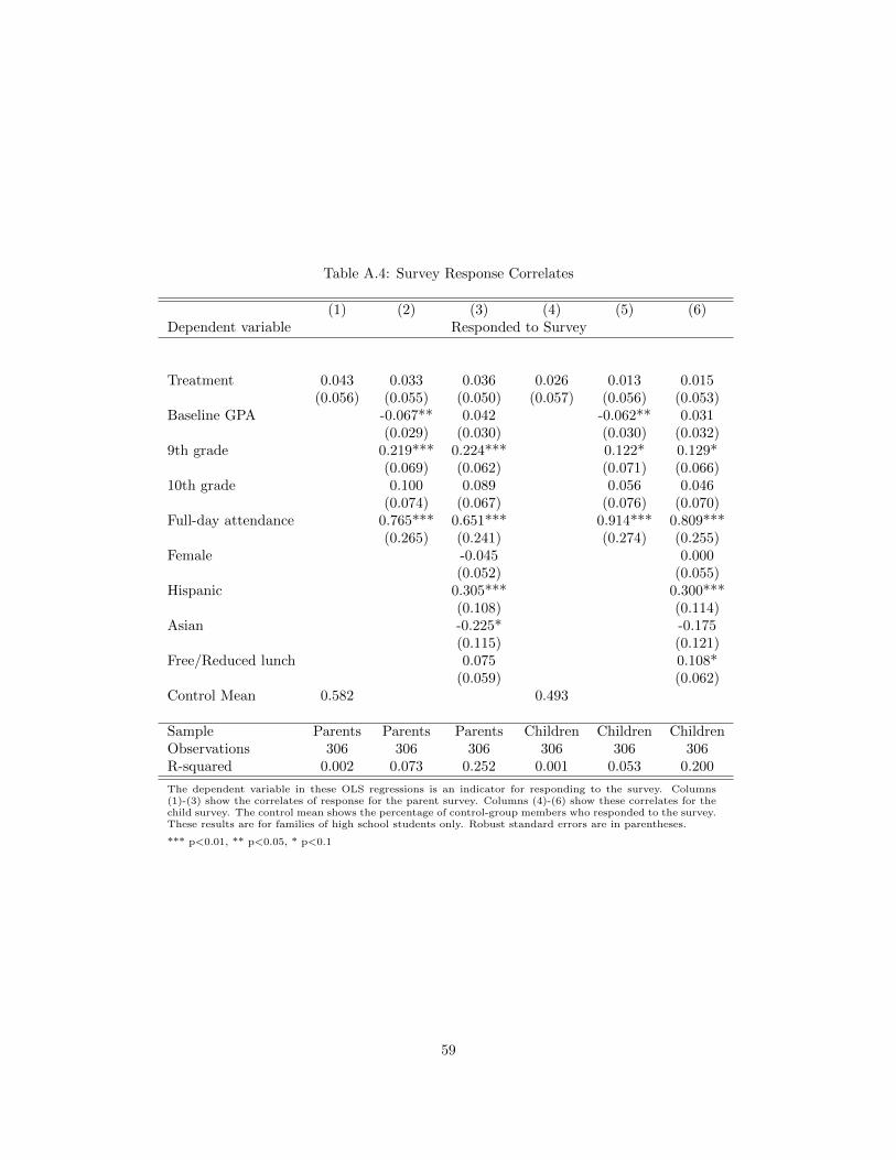
Table A.4: Survey Response Correlates

(1) (2) (3) (4) (5) (6)Dependent variable Responded to Survey

Treatment 0.043 0.033 0.036 0.026 0.013 0.015(0.056) (0.055) (0.050) (0.057) (0.056) (0.053)

Baseline GPA -0.067** 0.042 -0.062** 0.031(0.029) (0.030) (0.030) (0.032)

9th grade 0.219*** 0.224*** 0.122* 0.129*(0.069) (0.062) (0.071) (0.066)

10th grade 0.100 0.089 0.056 0.046(0.074) (0.067) (0.076) (0.070)

Full-day attendance 0.765*** 0.651*** 0.914*** 0.809***(0.265) (0.241) (0.274) (0.255)

Female -0.045 0.000(0.052) (0.055)

Hispanic 0.305*** 0.300***(0.108) (0.114)

Asian -0.225* -0.175(0.115) (0.121)

Free/Reduced lunch 0.075 0.108*(0.059) (0.062)

Control Mean 0.582 0.493

Sample Parents Parents Parents Children Children ChildrenObservations 306 306 306 306 306 306R-squared 0.002 0.073 0.252 0.001 0.053 0.200

The dependent variable in these OLS regressions is an indicator for responding to the survey. Columns(1)-(3) show the correlates of response for the parent survey. Columns (4)-(6) show these correlates for thechild survey. The control mean shows the percentage of control-group members who responded to the survey.These results are for families of high school students only. Robust standard errors are in parentheses.

*** p<0.01, ** p<0.05, * p<0.1

59

Table A.5: Missing CST Scores

(1) (2) (3) (4) (5) (6)

Dependentvariable

Missingmath

Missingmath

Missingmath

MissingEnglish

MissingEnglish

MissingEnglish

Treatment -0.054 -0.060* -0.065* -0.047 -0.051 -0.056(0.033) (0.033) (0.035) (0.032) (0.032) (0.035)

Baseline GPA -0.050* -0.041 -0.053* -0.050(0.028) (0.028) (0.021) (0.031)

Control mean 0.110 0.103

Additionalcontrols

No No Yes No No Yes

Observations 279 279 279 279 279 279R-squared 0 .010 0.010 0.122 0.008 0.090 0.173

The dependent variable in these OLS regressions is an indicator for having no test score. Additional controlsinclude prior GPA, prior scores, test-subject indicators and demographic characteristics. Robust standarderrors are in parentheses.

*** p<0.01, ** p<0.05, * p<0.1

60

Student Response Outside of School

The first three columns of Table 10 (Panel A) show how students’ work habits changed

outside of school. Tutoring attendance over the semester increased 42%. The coefficient

is marginally insignificant at standard levels (p-value equals .11). Tutoring was offered

by teachers after school for free. The positive effect on tutoring is at least partially due to

several teachers’ requirement that missing work be made up during their after school tutoring

to prevent cheating. The second column shows the effect on whether students did their

homework at the last minute, which was coded from zero to two for “never,” “sometimes” or

“always.” Students in the treatment group were significantly less likely to do their homework

at the last minute. Nonetheless, student study hours at home did not significantly increase,

which implies that most of the gains in achievement are due to improved work habits at

school.

The remaining two columns of Panel A show students’ valuations of schooling on a four-

point scale. Students in the treatment group are more likely to say grades are important,

but no more likely to say that college is important. While a generous interpretation may be

that students now intrinsically value schooling more, another interpretation of these results

is that grades are important because students will be punished if they do not do well, but

their intrinsic valuation of schooling has not changed. I cannot distinguish between these

interpretations however, but learning may develop regardless. Children’s myopia or discount

rates can change over time (Green et al., 1994), and perhaps having parents intercede until

a change may occur is nonetheless valuable. This interpretation would have implications

for longer-run results and the importance of extending the treatment over the longer time

periods, which is a limitation of this study.

61

Table A.6: Student Responses to Additional Information

How Students Responded Outside of School

Dependent variable TutoringHomeworklast minute Study hours

Gradesimportant

Collegeimportant

Treatment 5.978 -0.227* 0.146 0.234** 0.040(3.763) (0.116) (0.263) (0.102) (0.074)

Control Mean 14.250 1.202 0.380 3.681 3.639

Data source Child Child Child Child ChildObservations 154 152 153 155 154R-squared 0.086 0.087 0.160 0.181 0.133

All columns show the effects of the information treatment on parents. Treatment effects are estimated usingregressions that control for baseline GPA, prior GPA, strata indicators and grade-level indicators. Baseline GPAis GPA calculated from students’ mid-semester progress reports two months before the experiment began. PriorGPA is students’ cumulative GPA from middle school and beyond. Data source indicates whether the dependentvariable came from a parent’s survey response, a child’s survey response, or school records. Robust standard errorsare in parentheses.

*** p<0.01, ** p<0.05, * p<0.1

Table A.7: Peer Effects

(1)Dependent variable Class Grade

Fraction treated 0.578(0.500)

Observations 1042R-squared 0.417

This table shows how the fraction of the class treated affects class gradesfor the control group. This effect is calculated using an OLS regressionthat restricts the sample to the control group and controls for baselineGPA, GPA from a students prior school, grade-level indicators and strataindicators. Results are shown for high school students only. All data arefrom administrative records. Standard errors are clustered at the teacherlevel accounting for the 19 clusters using a Wild bootstrap t (Cameron,Gelbach, Miller, 2008) with 1000 repetitions.

*** p<0.01, ** p<0.05, * p<0.1

62

Table A.8: Multiple Testing Adjustment

Variable Significance

School contact to parent **Contacted more than once **School contact to parent **Contacted more than once **

GPA **Math Scores *English Scores -

Pr(Don’t know) *Pr(Missed 0-2) -Pr(Missed 3-5) *Pr(Missed 5+) -Difference from truth -Kid doesn’t disclose **

Contacted school **Attended conference -Ask HW -

Privileges *Talk college -Help kid -Can help **

Pr(in-class work habits unsatisfactory) ***Pr(in-class work habits excellent) ***Pr(in-class cooperation unsatisfactory) -Pr(in-class cooperation excellent) -Full-day rate attendance -By-class rate attendance -Classes missed -Pr(Missed assignment) **

Tutoring -HW last minute *Study hours -Grades important *College important -

Follow up GPA *Follow up Grades *

This table shows significance tests for treatment effects on each of the out-comes listed. Each outcome is grouped with a family of like outcomes andtest statistics are adjusted to strongly control for the Family-Wise ErrorRate using the step down method of Romano and Wolf (2005). Hypothesistests are two-sided against the null of zero effect.

*** p<0.01, ** p<0.05, * p<0.1, - p>0.1

63

Sample Selection and Test Scores

Ideally, state-mandated tests are administered to all students, which would help separate

out the treatment effect on participation from the effect on their score. Unfortunately, many

students did not take these tests, and as shown previously, missing a score is correlated

with treatment status and treatment-control imbalance—prior test scores of treatment-group

students are .26 lower and baseline GPA .13 points lower (results not shown). To see whether

those who did not take the test responded to the treatment differently than those who did

take the test, I compare the GPA results of those who took the standardized tests with those

who did not. Specifically, the indicator for treatment is interacted with an indicator for

having a math test score or English test score as follows.

GPAi = β0 + β1 ∗ Treatmenti + β2 ∗ Treatmenti ∗ 1(HasScorei) +X ′iγ + εi

Where the variable HasScorei is an indicator for either having an English test score or

having a math test score. The coefficient on the interaction term, β2, indicates whether

those who have a test score experienced different effects on GPA than those who do not have

a test score. This achievement effect might correlate with the achievement effect on test

scores. If β2 is large, it suggests how the test-score results might be biased—upwards if β2

is positive and downwards is β2 is negative.

Table A.9 below shows the results of this analysis. The coefficients on the interaction term

for having a score is insignificant (p-value equals .14) but is large and negative. Thus there

is some evidence that the treatment effect is smaller for those with test scores compared to

those without, which may bias the estimates on test scores downward.

64

Table A.9

(1)Dependent variable GPA

Treatment 0.700**(0.356)

Treatment*(has score) -0.546(0.369)

Observations 279R-squared 0.653

This table shows the treatment effect on GPA, and interacts the treatmentvariable with an indicator for whether or not a student has a math stan-dardized test score an English standardized test score. These effects areestimated with an OLS regression that controls for baseline GPA, GPAfrom a students prior school, grade-level indicators and strata indicators.Results are shown for high school students only. All data are from admin-istrative records. Robust standard errors in parentheses.

*** p<0.01, ** p<0.05, * p<0.1

65

C The Model

Derivations of PBE

I denote the student’s strategy as (type-H strategy; type-L strategy). I denote the parent’s

strategy as (after D = 1, after D = 0).

Separating Equilibria

Suppose the student’s strategy is (E = 1, D = 1;E = 0, D = 0).

1a. After D = 1, the parent knows t = H, and will monitor only U(M = 1) ≥ U(M = 0).

V − w −m+ εp(1) ≥ V − w + εp(0) =⇒ −m ≥ εp(0)− εp(1).

1b. After D = 0, the parent does not know the type. However, he updates his beliefs

about type P (H|D = 0) = (1−R)π1−Rπ . The parent will monitor if E(U(M = 1)|D = 0) ≥

E(U(M = 0)|D = 0).

(1−R)π

1−Rπ· (V − w −m)− 1− π

1−Rπ·m+ εp(1) ≥ (1−R)π

1−Rπ· (V − w)− 1− π

1−Rπ· w + εp(0)

=⇒ −m+1− π

1−Rπ· w ≥ εp(0)− εp(1)

Note that −m+ 1−π1−Rπ · w ≥ −m because w ≥ 0.

2. Case 1: −m+ 1−π1−Rπ · w ≥ −m ≥ εp(0)− εp(1) or (M = 1,M = 1).

– Then a type-H student will choose E = 1, D = 1 if w − cH + εi(1) ≥ εi(0) =⇒

w − cH ≥ εi(0)− εi(1).

– Then a type-L student will choose E = 0, D = 0 if εi(0) ≥ w − cL + εi(1) =⇒

εi(0)− εi(1) ≥ w − cL.

S1. There is an equilibrium at (M = 1,M = 1) and (E = 1, D = 1;E = 0, D = 0) if

w − cH ≥ εi(0)− εi(1) ≥ w − cL, and −m ≥ εp(0)− εp(1).

66

Case 2: −m+ 1−π1−Rπ · w ≥ εp(0)− εp(1) ≥ −m or (M = 0,M = 1).

– Then a type-H student will choose E = 1, D = 1 if w − cH + εi(1) ≥ εi(0) =⇒

w − cH ≥ εi(0)− εi(1)

– Then a type-L student will choose E = 0, D = 0 if εi(0) ≥ w − cL + εi(1) =⇒

εi(0)− εi(1) ≥ w − cL

S2. There is an equilibrium at (M = 0,M = 1) and (E = 1, D = 1;E = 0, D = 0) if

w − cH ≥ εi(0)− εi(1) ≥ w − cL, and −m+ 1−π1−Rπ · w ≥ εp(0)− εp(1) ≥ −m.

Case 3: εp(0)− εp(1) ≥ −m+ 1−π1−Rπ · w ≥ −m or (M = 0,M = 0).

– Then a type-H student will choose E = 1, D = 1 if w− cH + εi(1) ≥ w+ εi(0) =⇒

−cH ≥ εi(0)− εi(1).

– Then a type-L student will choose E = 0, D = 0 if w+ εi(0) ≥ w− cL + εi(1) =⇒

εi(0)− εi(1) ≥ −cL.

S3. Note that cH < cL. There is an equilibrium at (M = 0,M = 0) and (E = 1, D =

1;E = 0, D = 0) if εp(0)− εp(1) ≥ −m+ 1−π1−Rπ ·w, and −cH > εi(0)− εi(1) > −cL.

Suppose the student’s strategy is (E = 0, D = 0;E = 1, D = 1).

1a. After D = 1, the parent knows that t = L and will choose M = 1 if U(M = 1) ≥

U(M = 0) or

V − w −m+ εp(1) ≥ V − w + εp(0) =⇒ −m ≥ εp(0)− εp(1).

1b. After D = 0, the parent updates his beliefs on the about the student’s type.

P (H|D = 0) =P (D = 0|H)P (H)

P (D = 0|H)P (H) + P (D = 0|L)P (L)=

π

1−R +Rπ

67

Define P (H|D = 0) = p. Then the parent will not monitor if E(U(M = 0)|D = 0) ≥

E(U(M = 1)|D = 0).

p(−w) + (1− p)(V − w) + εp(0) ≥ p(−m) + (1− p)(V − w −m) + εp(1)

−pw + εp(0) ≥ −m+ εp(1)

εp(0)− εp(1) ≥ −m+π

1−R +Rπw

Note that −m+ π1−R+Rπ

w ≥ −m because w ≥ 0.

2. Case 1: −m+ π1−R+Rπ

w ≥ −m ≥ εp(0)− εp(1) or (M = 1,M = 1)

– Then type-H will not deviate if εi(0) ≥ w− cH +εi(1) =⇒ εi(0)−εi(1) ≥ w− cH .

– Then type-L will not deviate if w− cL + εi(1) ≥ εi(0) =⇒ εi(0)− εi(1) ≤ w− cL.

– Hence, this is not an equilibrium because cH < cL, so it cannot be the case that

w − cL ≥ εi(0)− εi(1) ≥ w − cH .

Case 2: −m+ π1−R+Rπ

w ≥ εp(0)− εp(1) ≥ −m or (M = 0,M = 1)

– Then type-H will not deviate if εi(0) ≥ w− cH +εi(1) =⇒ εi(0)−εi(1) ≥ w− cH .

– Then type-L will not deviate if w− cL + εi(1) ≥ εi(0) =⇒ εi(0)− εi(1) ≤ w− cL.

– Hence, this is not an equilibrium because cH < cL, so it cannot be the case that

w − cL ≥ εi(0)− εi(1) ≥ w − cH .

Case 3: εp(0)− εp(1) ≥ −m+ π1−R+Rπ

w ≥ −m or (M = 0,M = 0)

– Then type-H will not deviate if w+εi(0) ≥ w−cH+εi(1) =⇒ εi(0)−εi(1) ≥ −cH .

– Then type-L not deviate if w − cL + εi(1) ≥ w + εi(0) =⇒ −cL ≥ εi(0)− εi(1).

– Hence, this is not an equilibrium because cH < cL =⇒ −cH > −cL, so it cannot

be the case that −cL ≥ εi(0)− εi(1) ≥ −cH .

68

Pooling Equilibria

Suppose the student’s strategy is (E = 1, D = 1;E = 1, D = 1).

1a. After D = 1, knows that the student is exerting effort regardless of type. Nevertheless,

they pick M = 1 if U(M = 1) ≥ U(M = 0). That is, V − w −m + εp(1) ≥ V − w +

εp(0) =⇒ −m ≥ εp(0)− εp(1).

1b. After D = 0, then either a report has not been generated with probability 1−R or the

students are playing an off equilibrium strategy. The parent will update their beliefs as

follows:

P (H|D = 0) =P (H)P (D = 0|H)

P (H)P (D = 0|H) + P (L)P (D = 0|L)=

π(1−R)

π(1−R) + (1− π)(1−R)= π

The parent cannot update their beliefs. Therefore, they will monitor if U(M = 1) ≥

U(M = 0). That is, V − w −m+ εp(1) ≥ V − w + εp(0) =⇒ −m ≥ εp(0)− εp(1).

2. Case 1: −m ≥ εp(0)− εp(1) or (M = 1,M = 1).

– Then type-H will not deviate if w− cH +εi(1) ≥ εi(0) =⇒ w− cH ≥ εi(0)−εi(1).

– Then type-L will not deviate if w− cL + εi(1) ≥ εi(0) =⇒ w− cL ≥ εi(0)− εi(1).

P1. Then there is a pooling equilibrium at −m ≥ εp(0)−εp(1) and w−cL ≥ εi(0)−εi(1)

Case 2: εp(0)− εp(1) ≥ −m or (M = 0,M = 0).

– Then type-H will not deviate if w−cH+εi(1) ≥ w+εi(0) =⇒ −cH ≥ εi(0)−εi(1).

– Then type-L will not deviate if w−cL+εi(1) ≥ w+εi(0) =⇒ −cL ≥ εi(0)−εi(1).

P2. Then there is a pooling equilibrium at εp(0)− εp(1) ≥ −m and −cL ≥ εi(0)− εi(1)

Suppose the student’s strategy is (E = 0, D = 0;E = 0, D = 0).

69

1a. After D = 1, the parent sees that the student is playing off-equilibrium. He will monitor

if U(M = 1) ≥ U(M = 0) =⇒ V − w − m + εp(1) ≥ V − w + εp(0) =⇒ −m ≥

εp(0)− εp(1).

1b. After D = 0, the parent cannot update his beliefs. He will monitor if U(M = 1) ≥

U(M = 0) =⇒ −m + εp(1) ≥ −w + εp(0) =⇒ −m + w ≥ εp(0) − εp(1). Note that

w > 0 =⇒ −m+ w > −m.

2. Case 1: −m+ w ≥ −m ≥ εp(0)− εp(1) or (M = 1,M = 1).

– An H-type student will not deviate if εi(0) ≥ w − cH + εi(1) =⇒ εi(0)− εi(1) ≥

w − cH

– An L-type student will not deviate if εi(0) ≥ w − cL + εi(1) =⇒ εi(0) − εi(1) ≥

w − cL

P3. Note that w − cH ≥ w − cL, so there is an equilibrium at εi(0) − εi(1) ≥ w − cH

and −m ≥ εp(0)− εp(1).

Case 2: −m+ w ≥ εp(0)− εp(1) ≥ −m or (M = 0,M = 1).

– An H-type student will not deviate if εi(0) ≥ w − cH + εi(1) =⇒ εi(0)− εi(1) ≥

w − cH

– An L-type student will not deviate if εi(0) ≥ w − cL + εi(1) =⇒ εi(0) − εi(1) ≥

w − cL

P4. Note that w − cH ≥ w − cL, so there is an equilibrium at εi(0) − εi(1) ≥ w − cH

and −m+ w ≥ εp(0)− εp(1) ≥ −m

Case 3: εp(0)− εp(1) ≥ m+ w ≥ −m or (M = 0,M = 0).

– An H-type student will not deviate if w−εi(0) ≥ w−cH+εi(1) =⇒ εi(0)−εi(1) ≥

−cH

70

– An L-type student will not deviate if w−εi(0) ≥ w−cL+εi(1) =⇒ εi(0)−εi(1) ≥

−cL

P5. Hence, there is an equilibrium at εi(0)− εi(1) ≥ −cH and εp(0)− εp(1) ≥ m+ w.

Hybrid Equilibria

H1. Suppose the student’s strategy is (E = 1, D = 1; mix with P (E = 1, D = 1) = qL).

1a. After seeing D = 1, the parent updates his beliefs as follows:

P (H|D = 1) =P (D = 1|H)P (H)

P (D = 1|H)P (H) + P (D = 1|L)P (L)

=Rπ

Rπ +RqL(1− π)

=π

π + (1− π)qL

– The parent will be indifferent if E(U(M = 1)|D = 1) = E(U(M = 0)|D = 1) =⇒

V − w −m+ εp(1) = V − w + εp(0) =⇒ −m = εp(0)− εp(1).

1b. After seeing D = 0, the parent knows that either a report has not been generated, or

that the low type has not exerted effort.

P (H|D = 0) =P (D = 0|H)P (H)

P (D = 0|H)P (H) + P (D = 0|L)P (L)

=(1−R)π

(1−R)π + ((1−R)qL + (1− qL))(1− π)

= µ

– The parent will be indifferent after D = 0 if E(U(M = 1)|D = 0) = E(U(M =

0)|D = 0) =⇒ µ(V −w−m) + (1−µ)(qL(V −w−m) + (1− qL)(−m)) + εp(1) =

µ(V −w) + (1− µ)(qLV −w) + εp(0) =⇒ −m+ (1− µ)(1− qL)w = εp(0)− εp(1)

71

Case 1: −m = εp(0) − εp(1) =⇒ −m + (1− (µ1 + (1− µ1)qL))w > εp(0) − εp(1).

The parent’s strategy is (mix with α01 = P (M = 0|D = 1) after D = 1, M = 1 after

D = 0)

- The type-L student will be indifferent if EU(E = 1, D = 1) = EU(E = 0, D =

0) =⇒ w − cL + εi(1) = εi(0) =⇒ w − cL = εi(0)− εi(1).

- The type-H student will not deviate if EU(E = 1, D = 1) ≥ EU(E = 0, D =

0) =⇒ w − cH + εi(1) ≥ εi(0) =⇒ w − cH ≥ εi(0)− εi(1).

– Then there is an equilibrium if −m + (1− (µ1 + (1− µ1)qL))w > εp(0)− εp(1) =

−m,w − cH ≥ εi(0) − εi(1) = w − cL. However, as the probability of an event is

not defined at a point, this equilibrium occurs with probability 0.

Case 2: −m+ (1−µ)(1− qL)w = εp(0)− εp(1) =⇒ εi(0)− εi(1) > −m. The parent’s

strategy is (M = 0 after D = 1,mix after D = 0).

- The L-type student will be indifferent if EU(E = 1, D = 1) = EU(E = 0, D =

0) =⇒ w − cH + εi(1) = α00(w) + εi(0) =⇒ (1− α00)w − cL = εi(0)− εi(1).

- The H-type will not deviate if EU(E = 1, D = 1) ≥ EU(E = 0, D = 0) =⇒

w − cH + εi(1) ≥ α00w + εi(0) =⇒ (1− α00)w − cH ≥ εi(0)− εi(1).

H1. Then there is an equilibrium at −m+ (1−µ)(1− qL)w = εp(0)− εp(1)) > −m and

(1−α00)w− cH ≥ εi(0)− εi(1) = (1−α00)w− cL. Further, as α and qL both vary

between 0 and 1, −m+ 1−π1−Rπw ≥ εp(0)−εp(1)) ≥ −m, and w−cL ≥ εi(0)−εi(1) ≥

−cL.

Suppose the student’s strategy is (E = 0, D = 0; mix with P (E = 1, D = 1) = qL).

1a. After D = 1, the parent knows that the child must be a low type. Therefore, the parent

is indifferent if U(M = 1) = U(M = 0) =⇒ V − w −m+ εp(1) = V − w + εp(0) =⇒

−m = εp(0)− εp(0).

72

1b. After D = 0, the parent knows that either a report has not been generated for a hard

working L-type, or both types are not working.

P (H|D = 0) =P (D = 0|H)P (H)

P (D = 0|H)P (H) + P (D = 0|L)P (L)

=π

π + ((1−R)qL + (1− qL))(1− π)

= µ2

Then the parent is indifferent between monitoring and not monitoring if EU(M = 1) =

EU(M = 0) =⇒ µ2(−m) + (1 − µ2)(qL(V − w − m) + (1 − qL)(−m)) + εp(1) =

µ2(−w) + (1− µ2)(qL(V − w) + (1− qL)(−w)) =⇒ −m+ µqLw = εp(0)− εp(1)

Case 1: −m + µqLw ≥ εp(0) − εp(0) = −m. The parent’s strategy is (mix α01 after

D = 1,M = 1 after D = 0).

- The L-type student will mix if EU(E = 1, D = 1) = EU(E = 0, D = 0) =⇒

w − cL + εi(1) = εi(0) =⇒ w − cL = εi(0)− εi(1).

- The H-type student will not deviate if EU(E = 0, D = 0) ≥ EU(E = 1, D =

1) =⇒ εi(0) ≥ w − cH + εi(1) =⇒ εi(0)− εi(1) ≥ w − cH .

- However, w − cH > w − cL. Therefore, no equilibrium exists.

Case 2: −m + µqLw = εp(0) − εp(1) ≥ −m. The parent’s strategy is (M = 0 after

D = 1, mix after D = 0).

- The L-type will mix if EU(E = 1, D = 1) = EU(E = 0, D = 0) =⇒ w − cL +

εi(1) = α00w + εi(0) =⇒ (1− α00)w − cL = εi(0)− εi(1).

- The H-type student will not deviate if EU(E = 0, D = 0) ≥ EU(E = 1, D =

1) =⇒ α00w + εi(0) ≥ w − cH + εi(1) =⇒ εi(0)− εi(1) ≥ (1− α00)w − cH .

73

- However, (1− α00)w − cH > (1− α00)w − cL. Therefore, no equilibrium exists.

Suppose the student’s strategy is (mix with P (E = 1, D = 1) = qH ;E = 0, D = 0).

1a. After seeing D = 1, the parent knows that it must be the H-type student. Therefore,

he will mix if U(M = 1) = U(M = 0) =⇒ V − w −m + εp(1) = V − w + εp(0) =⇒

−m = εp(0)− εp(0).

1b. After seeing D = 0, the parent knows that either a report has not been generated for a

H-type student exerting effort with qH , or that neither type is exerting effort.

P (H|D = 0) =P (D = 0|H)P (H)

P (D = 0|H)P (H) + P (D = 0|L)P (L)

=((1−R)qH + (1− qH))π

((1−R)qH + (1− qH))π + (1− π)

= ν

The parent will mix if EU(M = 1) = EU(M = 0) =⇒ ν1(qH(V − w − m) + (1 −

qH)(−m))+(1−ν)(−m)+εp(1) = ν1(qH(V −w)+(1−qH)(−w))+(1−ν)(−w)+εp(0) =⇒

−m+ (1− νqH)w = εp(0)− εp(1).

Case 1: −m+ (1− ν1qH)w > εp(0)− εp(1) = −m. The parent’s strategy is (mix after

D = 1, M = 1 after D = 0)

- L-types will not deviate if E(U(E = 0)) ≥ E(U(E = 1)) =⇒ εi(0) ≥ w − cL +

εi(1) =⇒ εi(0)− εi(1) ≥ w − cL

- H-types will mix if E(U(E = 1)) = E(U(E = 0)) =⇒ w− cH + εi(1) = εi(0) =⇒

w − cH = εi(0)− εi(1)

- Then there is an equilibrium at −m+ (1−νqH)w > εp(0)− εp(1) = −m, w− cH =

εi(0)− εi(1) ≥ w − cL. However, as explained above, this equilibrium occurs with

probability 0.

74

Case 2: −m + (1 − νqH)w = εp(0) − εp(1) > −m. The parent’s strategy is (M = 1

after D = 1, mix after D = 0 with α00 = P (M = 0|D = 0))

- The L-type will not deviate if E(U(E = 0)) ≥ E(U(E = 1)) =⇒ α00w + εi(0) ≥

w − cL + εi(1) =⇒ εi(0)− εi(1) ≥ (1− α00)w − cL.

- The H-type will mix if E(U(E = 0)) = E(U(E = 1)) =⇒ α00w + εi(0) =

w − cH + εi(1) =⇒ (1− α00)w − cH = εi(0)− εi(1).

H2. Then there is an equilibrium at −m + (1 − νqH)w = εp(0) − εp(1) > −m and

(1−α00)w−cH = εi(0)−εi(1) ≥ (1−α00)w−cL. Further, as qH and α00 vary from

0 to 1, −m+w ≥ εp(0)−εp(1)) ≥ −m+ 1−π1−Rπw, and w−cH ≥ εi(0)−εi(1) ≥ −cH .

H4. Suppose the student’s strategy is (mix with P (E = 1, D = 1) = qH ;E = 1, D = 1).

1a. After seeing D = 1, the parent updates his beliefs.

P (H|D = 1) =P (D = 1|H)P (H)

P (D = 1|H)P (H) + P (D = 1|L)P (L)

=qHπ

qHπ + (1− π)

= γ1

Then the parent will mix if V −w−m+εp(1) = V −w+εp(0) =⇒ −m = εp(0)−εp(1).

1b. After seeing D = 0, the parent know that either a report was not generated or that the

H-type is playing E = 0, D = 0.

P (H|D = 1) =P (D = 1|H)P (H)

P (D = 1|H)P (H) + P (D = 1|L)P (L)

=(1−R)qHπ

((1− qH) + (1−R)qH)π + (1− π)

= γ2

75

Then the parent will mix if EU(M = 1) = EU(M = 0) =⇒ γ2(qH(V − w −m) + (1−

qH)(−m))+(1−γ2)(V −w−m)+εp(1) = γ2(qH(V −w)+(1−qH)(−w))+(1−γ2)(V −

w) + εp(0) =⇒ −m+ γ2(1− qH)w = εp(0)− εp(1).

Case 1: −m + γ2(1 − qH)w = εp(0) − εp(1) > −m The parent’s strategy is (M = 0

after D = 1,mix after D = 0 with α00 = P (M = 0|D = 0))

- The L-type will not deviate if EU(E = 1) ≥ EU(E = 0) =⇒ w − cL + εi(1) ≥

α00w + εi(0) =⇒ (1− α00)w − cL ≥ εi(0)− εi(1).

- The H-type will mix if EU(E = 1) ≥ EU(E = 0) =⇒ w − cH + εi(1) =

α00w + εi(0) =⇒ (1− α00)w − cH = εi(0)− εi(1).

- Then there is no equilibrium because w − cH ≥ w − cL.

Case 2:−m + γ2(1 − qH)w > εp(0) − εp(1) = −m The parent’s strategy is (mix after

D = 1, M = 1 after D = 0)

- The L-type will not deviate if EU(E = 1) ≥ EU(E = 0) =⇒ w − cL + εi(1) ≥

εi(0) =⇒ w − cL ≥ εi(0)− εi(1).

- The H-type will mix if EU(E = 1) = EU(E = 0) =⇒ w− cH + εi(1) = εi(0) =⇒

w − cH = εi(0)− εi(1).

- Then there is no equilibrium because w − cH ≥ w − cL.

Constructing Probabilities

First, I define the probability for each set of actions, a = (M,E,D), and equilibrium. To

derive these probabilities, I multiply the probability of an action given the parameters θ

and the equilibrium that occurs, P (a|Eq, θ), by the probability that the equilibrium occurs,

P (Eq). For example, the probability of a = (1, 1, 1) given the first separating equilibrium

in the appendix, S1, is the probability that a high type is drawn and a report is generated.

76

The probability that equilibrium S1 is drawn is (Φ(w− cH)−Φ(w− cL))Φ(−m) where Φ(·)

is the cumulative normal distribution function.

The joint probabilities for these actions and separating equilibria S1 − S3 and pooling

equilibria P1− P5 are defined as follows, letting γ = 1−π1−Rπ to condense notation:

P (1, 1, 1, S1|θ) = πR(Φ(w − cH)− Φ(w − cL))Φ(−m)

P (1, 1, 0, S1|θ) = π(1−R)(Φ(w − cH)− Φ(w − cL))Φ(−m)

P (1, 0, 0, S1|θ) = (1− π)(Φ(w − cH)− Φ(w − cL))Φ(−m)

P (0, 1, 1, S2|θ) = πR(Φ(w − cH)− Φ(w − cL))(Φ(−m+ γw)− Φ(−m))

P (1, 1, 0, S2|θ) = π(1−R)(Φ(w − cH)− Φ(w − cL))(Φ(−m+ γw)− Φ(−m))

P (1, 0, 0, S2|θ) = (1− π)(Φ(w − cH)− Φ(w − cL))(Φ(−m+ γw)− Φ(−m))

P (0, 1, 1, S3|θ) = πR(Φ(−cH)− Φ(−cL))(1− Φ(−m+ γw))

P (0, 1, 0, S3|θ) = π(1−R)(Φ(−cH)− Φ(−cL))(1− Φ(−m+ γw))

P (0, 0, 0, S3|θ) = (1− π)(Φ(−cH)− Φ(−cL))(1− Φ(−m+ γw))

P (1, 1, 1, P1|θ) = R(Φ(w − cL))Φ(−m)

P (1, 1, 0, P1|θ) = (1−R)Φ(w − cL)Φ(−m)

P (0, 1, 1, P2|θ) = RΦ(−cL)(1− Φ(−m))

P (0, 1, 0, P2|θ) = (1−R)Φ(−cL)(1− Φ(−m))

P (1, 0, 0, P3|θ) = (1− Φ(w − cH))Φ(−m)

P (1, 0, 0, P4|θ) = (1− Φ(w − cH))(Φ(−m+ w)− Φ(−m))

P (0, 0, 0, P5|θ) = (1− Φ(−cH))(1− Φ(−m+ w))

For the hybrid equilibria, H1, the probability of the outcome a = (0, 0, 0), given εi(0) −

εi(1) and εp(0) − εp(1), is the probability of drawing a low type, 1-π, multiplied by the

77

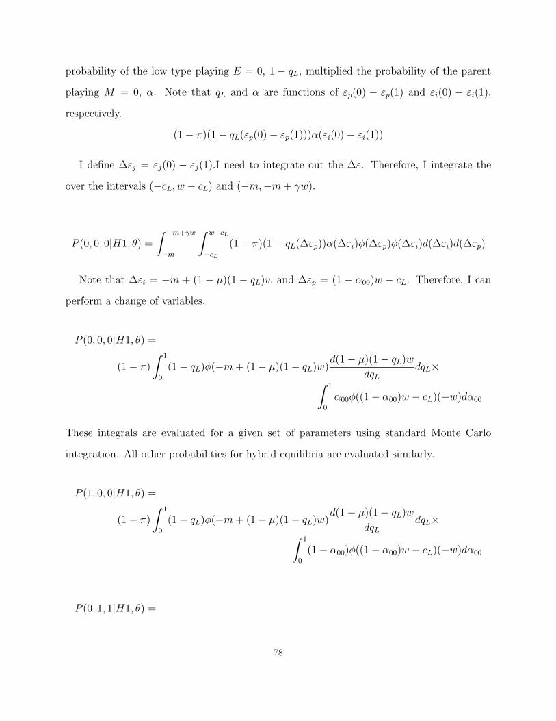
probability of the low type playing E = 0, 1 − qL, multiplied the probability of the parent

playing M = 0, α. Note that qL and α are functions of εp(0) − εp(1) and εi(0) − εi(1),

respectively.

(1− π)(1− qL(εp(0)− εp(1)))α(εi(0)− εi(1))

I define ∆εj = εj(0) − εj(1).I need to integrate out the ∆ε. Therefore, I integrate the

over the intervals (−cL, w − cL) and (−m,−m+ γw).

P (0, 0, 0|H1, θ) =

∫ −m+γw

−m

∫ w−cL

−cL(1− π)(1− qL(∆εp))α(∆εi)φ(∆εp)φ(∆εi)d(∆εi)d(∆εp)

Note that ∆εi = −m + (1 − µ)(1 − qL)w and ∆εp = (1 − α00)w − cL. Therefore, I can

perform a change of variables.

P (0, 0, 0|H1, θ) =

(1− π)

∫ 1

0

(1− qL)φ(−m+ (1− µ)(1− qL)w)d(1− µ)(1− qL)w

dqLdqL×∫ 1

0

α00φ((1− α00)w − cL)(−w)dα00

These integrals are evaluated for a given set of parameters using standard Monte Carlo

integration. All other probabilities for hybrid equilibria are evaluated similarly.

P (1, 0, 0|H1, θ) =

(1− π)

∫ 1

0

(1− qL)φ(−m+ (1− µ)(1− qL)w)d(1− µ)(1− qL)w

dqLdqL×∫ 1

0

(1− α00)φ((1− α00)w − cL)(−w)dα00

P (0, 1, 1|H1, θ) =

78

∫ 1

0

(R(π + (1− π)qL)φ(−m+ (1− µ)(1− qL)w)d(1− µ)(1− qL)w

dqLdqL×∫ 1

0

φ((1− α00)w − cL)(−w)dα00

P (0, 1, 0|H1, θ) =∫ 1

0

((1−R)π + (1−R)(1− π)qL)φ(−m+ (1− µ)(1− qL)w)d(1− µ)(1− qL)w

dqLdqL×∫ 1

0

α00φ((1− α00)w − cL)(−w)dα00

P (1, 1, 0|H1, θ) =∫ 1

0

((1−R)π + (1−R)(1− π)qL)φ(−m+ (1− µ)(1− qL)w)d(1− µ)(1− qL)w

dqLdqL×∫ 1

0

(1− α00)φ((1− α00)w − cL)(−w)dα00

P (0, 0, 0|H2, θ) =∫ 1

0

((1− π) + π(1− qH))φ(−m+ (1− νqH)w)d(1− ν)qHw

dqHdqH×∫ 1

0

α00φ((1− α00)w − cH)(−w)dα00

P (1, 0, 0|H2, θ) =∫ 1

0

((1− π) + π(1− qH))φ(−m+ (1− νqH)w)d(1− ν)qHw

dqHdqH×∫ 1

0

(1− α00)φ((1− α00)w − cH)(−w)dα00

79

P (1, 1, 1|H2, θ) = ∫ 1

0

(πRqH)φ(−m+ (1− νqH)w)d(1− ν)qHw

dqHdqH×∫ 1

0

φ((1− α00)w − cH)(−w)dα00

P (1, 1, 0|H2, θ) =∫ 1

0

(π(1−R)qH)φ(−m+ (1− νqH)w)d(1− ν)qHw

dqHdqH×∫ 1

0

(1− α00)φ((1− α00)w − cH)(−w)dα00

P (0, 1, 0|H2, θ) =∫ 1

0

(π(1−R)qH)φ(−m+ (1− νqH)w)d(1− ν)qHw

dqHdqH×∫ 1

0

α00φ((1− α00)w − cH)(−w)dα00

The probability of each event a is just the sum of the equilibrium conditional probabilities

of the event.

P (a|θ) =∑e∈EQ

P (a|e, θ, π)

80

Estimation

Uniqueness of equilibria means that there is a well-defined likelihood function. Let j be the

observation. The likelihood function is

logL((mp, ei, di)|θ) =1

n

n∑j=1

(mpjeijdij logP ((1, 1, 1)|θ) +mpjeij(1− dij) logP ((1, 1, 0)|θ)

+mpj(1− eij)(1− dij) logP ((1, 0, 0)|θ)

+ (1−mpj)eijdij logP ((0, 1, 1)|θ)

+ (1−mpj)eij(1− dij) logP ((0, 1, 0)|θ)

+ (1−mpj)(1− eij)(1− dij)P ((0, 0, 0)|θ)))

Clearly, V is not identified. Furthermore, there are a number of issues in identifying w, cL,

and cH . To illustrate, suppose that w = 0. (Notice that this implies that there are no hybrid

equilibria.) Then the probabilities of particular events reduce to

P (1, 1, 1|θ) = R(πΦ(−cH) + (1− π)Φ(−cL))Φ(−m)

P (1, 1, 0|θ) = (1−R)(πΦ(−cH) + (1− π)Φ(−cL))Φ(−m)

P (1, 0, 0|θ) = −(πΦ(−cH) + (1− π)Φ(−cL))Φ(−m) + Φ(−m)

P (0, 1, 1|θ) = R(πΦ(−cH) + (1− π)Φ(−cL))(1− Φ(−m))

P (0, 1, 0|θ) = (1−R)(πΦ(−cH) + (1− π)Φ(−cL))(1− Φ(−m))

P (0, 0, 0|θ) = −(πΦ(−cH) + (1− π)Φ(−cL))(1− Φ(−m)) + (1− Φ(−m))

Let πΦ(−cH) + (1− π)Φ(−cL) = η. Then this system of equations reduces to

P (1, 1, 1|θ) = RηΦ(−m)

P (1, 1, 0|θ) = (1−R)ηΦ(−m)

81

P (1, 0, 0|θ) = −ηΦ(−m) + Φ(−m)

P (0, 1, 1|θ) = Rη(1− Φ(−m))

P (0, 1, 0|θ) = (1−R)η(1− Φ(−m))

P (0, 0, 0|θ) = −η(1− Φ(−m)) + (1− Φ(−m))

I can pin down Φ(−m), η, and R using the above equations. However, I cannot pin down π,

cH , and cL individually.

This problem carries over to the case that w > 0. If the probability of a hybrid equilibria

is small, then P (1, 1, 1|θ) is close to a linear combination of P (0, 1, 1|θ). If γ is close to

one, then P (1, 1, 0|θ) is close to a linear combination of P (1, 0, 0|θ). P (0, 0, 0|θ) is close to

a linear combination of P (0, 1, 0|θ) if w is small and the probability of hybrid equilibria is

small. Under these conditions it is difficult to identify w, cL, cH .

Distribution of Equilibria and Model Fit

Table A.10: Distribution of Equilibria for Treatment and Control Groups

Equilibrium Control Distribution Treatment Distribution

S1 0.15972 0.19879S2 0.31243 0.29546S3 0.04625 0.00923

P1 0.15955 0.19854P2 0.00094 0.00083P3 0.00002 0.00002P4 0.00002 0.00002P5 0.00092 0.00051

H1 0.31231 0.29537H2 0.00784 0.00124

Note: This table shows the distribution of equilibria estimated for the treatmentand control groups, respectively. Each equilibrium (S1, S2, etc.) corresponds toan equilibrium labeled as such in the derivations below.

82

Table A.11: Simulated Moments Compared to Observed Moments

Variable Model Observed

Treatment Group

Monitor 0.766 0.743Effort 0.544 0.548Disclosure 0.363 0.387

Control Group

Monitor 0.731 0.717Effort 0.501 0.512Disclosure 0.320 0.356

Note: This table shows the distribution of equi-libria estimated for the treatment and controlgroups, respectively. Each equilibrium (S1, S2,etc.) corresponds to an equilibrium labeled assuch in the derivations below.

83

D Middle School Results

Table A.12 summarizes the effects on achievement and effort-related outcomes for middle

school students, which are mostly small and not significantly different from zero. These

results are consistent with the effects on how parents used the additional information, how

children responded, and parents’ awareness and demand for information (Table A.13). Based

on these results and the contamination, it is difficult to discern what effect the treatment

would have had on younger students.

There are several reasons the additional information may have had less effect on younger

children. First, the middle school students have less margin to improve: Their GPA is almost

a full standard deviation higher than high school students’ GPA, middle school students miss

7.5% of their assignments compared to high school students who miss 20% of their assign-

ments, and attendance and behavior are also better for middle school students. However if

this were the only cause for small effects, there could still be an impact on students who

were lower-performing at baseline. Unfortunately the study is underpowered to examine sub-

groups in the middle school, but point estimates show students with higher GPA respond

more positively to additional information (results not shown).

A second reason there might be smaller effects for middle school students is that parents

might be able to control younger children better than older children. It might be less costly

for parents to motivate their children or information problems arise less frequently. There

is some support for this hypothesis since teacher-measured behavior at baseline is better

for middle school students than high school students, which might correlate with parents’

ability to control their child. Third, the repeated messages to middle school parents through

the information treatment and the contamination by the school employee may have annoyed

them. If they had already resolved an issue such as a missing assignment, receiving a second

message regarding that work might have been confusing and frustrating. Parents could have

viewed the information treatment as less reliable given the lack of coordination about school-

84

to-parent contact and started ignoring it, which might explain the small negative coefficients

on several middle school outcomes.

Lastly, parents of middle-school students might already obtain information about their

child’s education more actively, which is reflected in the higher parent-teacher conference

attendance. In addition, a comparison of the control groups in the high school and middle

school shows that parents of middle school students are more likely to take away privileges

from their children, be aware of information problems, contact the school about their child’s

grades, and feel that they can help their child try their best than parents of high school

students in the control group.32 It is possible that the contamination caused this higher

level of involvement—meaning messages home did affect middle school parents—or it could

be that these parents were already more involved than high school parents. If the latter, it

leaves open the question of why this involvement wanes as children get older; perhaps parents

perceive they have less control of their child’s effort or that they no longer know how to help

them. In short, the effect of additional information on younger children is inconclusive.

32Results available upon request.

85

Table A.12: Middle School Student Outcomes

Dependent Variable Treatment Standard Error Students Observations

GPA -0.108 (0.102) 149 149Final Exams -0.054 (0.199) 87 87Math CST 0.034 (0.119) 139 139English CST -0.017 (0.13) 145 145Pr(missed assignment) 0.005 (0.01) 87 7,692Work habits unsatisfactory 0.019 (0.019) 149 2,635Work habits excellent -0.041 (0.039) 149 2,635Cooperation unsatisfactory 0.004 (0.009) 149 2,635Cooperation excellent -0.021 (0.038) 149 2,635Full-day attendance -1.101 (0.684) 149 148By-class attendance -1.918 (1.24) 149 1,933Classes missed 0.782 (0.49) 149 1,933

This table summarizes the results of the treatment effects on middle-school student outcomes, where the experimentwas contaminated. The results shown are the coefficients on the treatment indicator in a regression that controls forbaseline GPA, prior GPA, grade-level indicators and strata indicators. The treatment effect on missing an assignment isthe marginal effect at the means from a Probit model. Work habits and cooperation treatment effects are the marginaleffects at the means from an ordered Probit model. All remaining results are estimated by OLS. Where the number ofobservations differs from the number of students, this is because each student receives a behavior mark for each class aswell as each of the four grading periods. By-class attendance is an end-of-semester measure given for each class a studenttakes. The data for these regressions are drawn from administrative records. Final exam scores could not be obtained forthe sixth grade. Standard errors clustered by student are in parentheses.

*** p<0.01, ** p<0.05, * p<0.1

86

Table A.13: Middle School Family Survey Outcomes

Dependent Variable Treatment Standard Error N

Contact from the Schools

School Contact to parent 1.445*** (0.350) 80Contacted more than once 0.308*** (0.111) 80

How Parents Used the Information

Privileges taken last month 0.260 (0.320) 79Talk about college -0.548 (1.325) 82Ask about homework -4.532 (2.745) 81Help with homework -0.186* (0.111) 65

How Students responded

Tutoring 0.845 (1.500) 65HW last minute -0.001 (0.120) 64Study hours -0.267 (0.322) 60Grades important -0.167 (0.190) 65College important -0.152 (0.135) 65

Information Problems and Information Demand

Information problem? 0.100 (0.089) 80Contacted School -0.460 (0.601) 81Can help 0.060 (0.077) 82

The dependent variables in these OLS regressions are from parent and studentsurveys. Additional controls in these regressions are baseline GPA, grade-levelindicators and strata indicators. These results are for families of middle schoolstudents only, where the experiment was contaminated. Robust standard errorsare in parentheses.

*** p<0.01, ** p<0.05, * p<0.1

87