Parasite sources and sinks in a patchedRoss-Macdonald malaria model with human andmosquito movement: implications for control

Nick W. Ruktanonchai∗, David L. Smith†, and Patrick De Leenheer‡

July 14, 2016

Abstract

We consider the dynamics of a mosquito-transmitted pathogen in a multi-patch Ross-Macdonald malaria model with mobile human hosts, mobile vec-tors, and a heterogeneous environment. We show the existence of a globallystable steady state, and a threshold that determines whether a pathogen iseither absent from all patches, or endemic and present at some level in allpatches. Each patch is characterized by a local basic reproduction number,whose value predicts whether the disease is cleared or not when the patchis isolated: patches are known as “demographic sinks” if they have a localbasic reproduction number less than one, and hence would clear the disease ifisolated; patches with a basic reproduction number above one would sustainendemic infection in isolation, and become “demographic sources” of para-sites when connected to other patches. Sources are also considered focal areasof transmission for the larger landscape, as they export excess parasites toother areas and can sustain parasite populations. We show how to deter-mine the various basic reproduction numbers from steady state estimates inthe patched network and knowledge of additional model parameters, herebyidentifying parasite sources in the process. This is useful in the context ofcontrol of the infection on natural landscapes, because a commonly suggestedstrategy is to target focal areas, in order to make their corresponding basicreproduction numbers less than one, effectively turning them into sinks. Weshow that this is indeed a successful control strategy -albeit a conservativeand possibly expensive one- in case either the human host, or the vector doesnot move. However, we also show that when both humans and vectors move,this strategy may fail, depending on the specific movement patterns exhibitedby hosts and vectors.

∗University of Southampton, nrukt00@gmail.com†Institute for Health Metrics and Evaluation, Department of Global Health, University of Wash-

ington, Seattle WA, smitdave@gmail.com‡Department of Mathematics and Department of Integrative Biology, Oregon State University,

deleenhp@math.oregonstate.edu. Partially supported by NSF DMS grant 1411853.

1

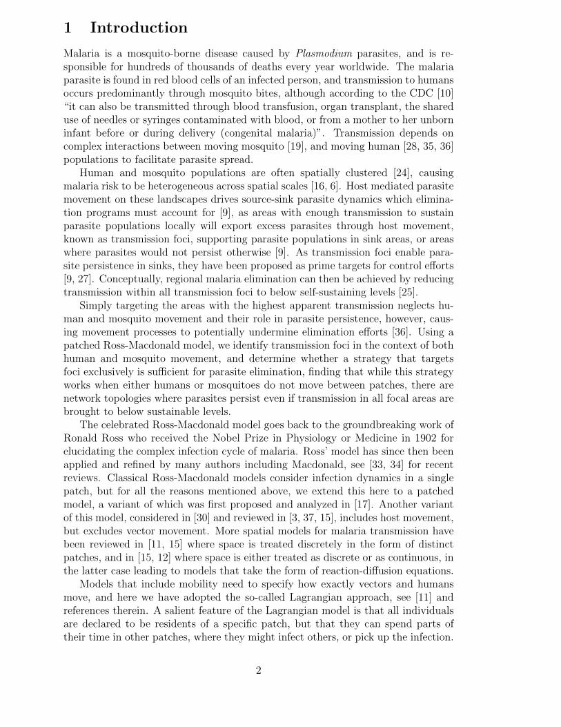
1 Introduction

Malaria is a mosquito-borne disease caused by Plasmodium parasites, and is re-sponsible for hundreds of thousands of deaths every year worldwide. The malariaparasite is found in red blood cells of an infected person, and transmission to humansoccurs predominantly through mosquito bites, although according to the CDC [10]“it can also be transmitted through blood transfusion, organ transplant, the shareduse of needles or syringes contaminated with blood, or from a mother to her unborninfant before or during delivery (congenital malaria)”. Transmission depends oncomplex interactions between moving mosquito [19], and moving human [28, 35, 36]populations to facilitate parasite spread.

Human and mosquito populations are often spatially clustered [24], causingmalaria risk to be heterogeneous across spatial scales [16, 6]. Host mediated parasitemovement on these landscapes drives source-sink parasite dynamics which elimina-tion programs must account for [9], as areas with enough transmission to sustainparasite populations locally will export excess parasites through host movement,known as transmission foci, supporting parasite populations in sink areas, or areaswhere parasites would not persist otherwise [9]. As transmission foci enable para-site persistence in sinks, they have been proposed as prime targets for control efforts[9, 27]. Conceptually, regional malaria elimination can then be achieved by reducingtransmission within all transmission foci to below self-sustaining levels [25].

Simply targeting the areas with the highest apparent transmission neglects hu-man and mosquito movement and their role in parasite persistence, however, caus-ing movement processes to potentially undermine elimination efforts [36]. Using apatched Ross-Macdonald model, we identify transmission foci in the context of bothhuman and mosquito movement, and determine whether a strategy that targetsfoci exclusively is sufficient for parasite elimination, finding that while this strategyworks when either humans or mosquitoes do not move between patches, there arenetwork topologies where parasites persist even if transmission in all focal areas arebrought to below sustainable levels.

The celebrated Ross-Macdonald model goes back to the groundbreaking work ofRonald Ross who received the Nobel Prize in Physiology or Medicine in 1902 forelucidating the complex infection cycle of malaria. Ross’ model has since then beenapplied and refined by many authors including Macdonald, see [33, 34] for recentreviews. Classical Ross-Macdonald models consider infection dynamics in a singlepatch, but for all the reasons mentioned above, we extend this here to a patchedmodel, a variant of which was first proposed and analyzed in [17]. Another variantof this model, considered in [30] and reviewed in [3, 37, 15], includes host movement,but excludes vector movement. More spatial models for malaria transmission havebeen reviewed in [11, 15] where space is treated discretely in the form of distinctpatches, and in [15, 12] where space is either treated as discrete or as continuous, inthe latter case leading to models that take the form of reaction-diffusion equations.

Models that include mobility need to specify how exactly vectors and humansmove, and here we have adopted the so-called Lagrangian approach, see [11] andreferences therein. A salient feature of the Lagrangian model is that all individualsare declared to be residents of a specific patch, but that they can spend parts oftheir time in other patches, where they might infect others, or pick up the infection.

2

This is in contrast to the more popular Eulerian approach, where individuals arenot assigned to a particular patch, but instead simply move around between thevarious patches at certain prescribed rates. Examples of the Eulerian approachcan be found in various contexts related to the spread of infectious diseases suchas in [1, 2, 5, 11], and are not restricted to malaria. Our methods can be usedto study similar patched Ross-Macdonald models based on the Eulerian approach,but to keep our analysis concise, we restrict ourselves to models based on the lessfrequently used Lagrangian approach. More sophisticated patch models have beenproposed more recently. These models have been coupled to agent-based modelsto incorporate movement of the individual agents (both vectors and humans) inresponse to other environmental triggers such as temperature or rainfall, revealingfascinating patterns in the numerical simulations of these hybrid systems, see [23].The main contributions of this paper are:

1. Establish the global dynamics of a patched Ross-Macdonald model,a variant of which was first investigated in [17] and reviewed in [11]. Thismodel assumes an arbitrary number of patches between which both humansand mosquitoes are allowed to move. These movement patterns are quantifiedby matrices which express the fractions of time spent by residents of eachpatch in all other patches. A single real and positive quantity -the spectralradius of a matrix defined in terms of model parameters of all patches, as wellas the movement matrices- determines the fate of the infection in the network:When this spectral radius is less than one, the infection is cleared. When itis larger than one, all solutions converge to a unique positive steady state andthe infection globally persists in all the patches.

Although our proof is based on techniques that are similar to those used in[11] for a closely related model, we have decided to include a concise andself-contained proof in an Appendix here, for two main reasons. First, thereare important differences between the modeling assumptions made in [17],and those considered here. Secondly, our proof relies on specific irreducibilityproperties of the matrices that encode vector and host mobility, and theseconditions are different from those stated in [11], in a rather subtle way.

2. Identify local sinks and sources from steady state measurementsof infected humans in the network. Each patch in the patched Ross-Macdonald model has its own transmission characteristics. In fact, to eachpatch we can associate a basic reproduction number, which would predictinfection persistence or clearance in this patch if the patch were isolated. Sincecontrol measures are often aimed at lowering the reproduction numbers ofthose patches with the highest reproduction number values, an obvious firststep is to determine, or at least estimate, the basic reproduction numbers ofevery patch with as little knowledge of model parameter values as possible.We show how to do this, based on the steady state measurements of infectedhumans in all the patches of the network. It turns out that only a limitednumber of model parameters is needed to achieve this, and we precisely statewhich ones these are.

3. Investigate how the patch reproduction numbers, in conjunction

3

with host and vector mobility patterns, affect disease persistenceor clearance in the network. We first consider the special cases whereeither only humans, or only mosquitoes move. If all patches are hotspots (re-spectively, sinks), then no matter what the mobility pattern of the moving hostis, the disease persists in (respectively, is cleared from) the network. Thus, thecontrol strategy that makes the reproduction number of every patch less thanone, is guaranteed to clear the infection from the network, no matter whatthe mobility pattern of the moving host is. However, when there is a mix ofhotspots and sinks in the network, this control strategy might be too conser-vative: For some mobility patterns the infection might be cleared without anyintervention, although it may persist for others. This also indicates that inthis case, an alternative control strategy -namely to intervene in the mobilitypatterns of the hosts- might be sufficient to clear the infection; and it mayeven be a cheaper one in certain cases, in particular when imposing travelrestrictions is more cost-effective. We end by considering the general scenarioin which both humans and mosquitoes move. A striking difference, comparedto the cases where only one population moves, is that now the control strategythat makes the basic reproduction numbers less than one in all patches, mayfail to clear the infection from the network. Failure or success depends on themobility patterns of both humans and mosquitoes. Similarly, it may happenthat in a network consisting of only sources, the infection is cleared by itself,without any control intervention at all. These results indicate that controllinga malaria infection in a network depends in a subtle way on the interplay be-tween local transmission characteristics in the patches on the one hand, andthe movement patterns of both hosts on the other.

The rest of this paper is organized as follows. In Section 2 we introduce the patchedRoss-Macdonald model and discuss its global behavior. Two Appendices containthe proof of this result. In Section 2 we also propose a solution to the problem ofdetermining the local reproduction numbers of all the patches based on steady statemeasurements. In Section 3 we investigate how patch characteristics, together withmobility patterns of vectors and human hosts, affect disease clearance or persistencein the network. Implications for control strategies aimed at clearing the infectionfrom the network are considered here as well. Finally, we conclude this paper withsome remarks in Section 4.

2 Malaria models

2.1 Single patch

The core model on which we later base our patched model, is a (rescaling of a) singlepatch Ross-Macdonald model proposed in [33], see also [11, 34] :

X = ab e−µτ Y

(H −XH

)− rX (1)

Y = acX

H(V − Y )− µY (2)

4

This model represents the dynamics for the number of infected humans X, and thenumber of infected mosquitoes Y in a total human population of H, and a totalmosquito population of V individuals. Individuals in both populations are assumedto be either susceptible, or infected. Hence, the number of susceptible humans isH −X, and the number of susceptible mosquitoes is V − Y . The other parametersin this model are:

1. r is the recovery rate of infected humans, and µ is the death rate of mosquitoes,both having units of 1/time.

2. a is the biting rate of mosquitoes with units of number of humans bitten permosquito and per unit of time.

3. τ is the incubation period (in units of time), i.e. the expected time that elapsesbetween the moment a mosquito picks up the infection, and the moment itbecomes infectious. When τ is non-negligible compared to the expected life-time of a mosquito 1/µ, it may happen that an infected mosquito dies beforeit becomes infectious. Thus, whereas Y is the number of infected mosquitoes,e−µτ Y represents the number of infectious mosquitoes which are capable ofinfecting susceptible humans. This explains the appearance of the exponentialfactor in equation (1).

4. b and c represent the probability that a bite by an infectious mosquito infectsa susceptible human, and the probability that a bite by a susceptible mosquitoof an infected human is successful, respectively.

Clearly, the first term in (1) and in (2) represents the infection rate of susceptiblehumans, and of susceptible mosquitoes, and the remaining terms in these equationsare the (human) recovery rate, and the (mosquito) death rate.

We scale X and Y :

x =X

H, y =

Y

V, (3)

and obtain the proportions of infected humans x and of infected mosquitoes y. Wealso introduce the ratio of the total number of mosquitoes over the total number ofhumans:

m =V

H, (4)

and then the dynamics for the proportions x and y is given by:

x = mab e−µτ y (1− x)− rx (5)

y = acx(1− y)− µy (6)

Defining the basic reproduction number1 following [33]:

R0 =ma2bc e−µτ

rµ(7)

=mabα e−µτ

r(8)

1Note that if one applies the procedure in [13] to calculate the basic reproduction number, oneobtains the square root of the expression on the right-hand side of (7). Note also that no matterwhich definition one uses, the statement of Theorem 1 describing the global behavior of the system,remains the same.

5

whereα =

ac

µ(9)

is the probability that a susceptible mosquito is infected during its life time. We seethat (5)− (6) has a unique steady state (x, y):

x =R0 − 1

R0 + α, y =

α(R0 − 1)

(α + 1)R0

(10)

in (0, 1)2 if and only if R0 > 1. Note also that (0, 0) is always a steady state of(1)− (2).

The following global result can be proved using standard phase plane techniques,see [20] for instance. Alternatively, one could exploit the monotonicity of the system,see [32], as well as the Appendix, for more on monotone systems:

Theorem 1. If R0 < 1, then all solutions of (5)− (6) converge to (0, 0). If R0 > 1,then all positive solutions of (5)− (6) converge to (x, y).

Estimating R0. We now turn to the question of how to estimate the value of R0,using steady state measurements of the fraction of infected humans only. It turnsout that additional information is needed, but that Theorem 1 readily provides theanswer:

1. If R0 > 1, then estimating R0 based on observing the steady state value x,and the knowledge of α, is possible by simply inverting (10):

R0 =1 + αx

1− x, (11)

2. But if R0 < 1, then the observed steady state is (0, 0). In this case, the valueof R0 cannot be estimated by observing the (0, 0) steady state, even if α isknown.

Control measures. To clear the infection, one must make R0 less than 1, andin view of formula (7) this may be achieved by lowering m, a, b and c (or α), orincreasing r, µ and τ . Practical control strategies could include the use of screens,bednets and repellents (decreases a), drug treatment (increases r), use insecticides(increases µ and decreases m), vaccination (decreases b), larval source management(decreases m), and relocation of humans (decreases m).

2.2 Multi-patch

Suppose that there are n patches and that in each patch the disease dynamics obeysthe Ross-Macdonald model (1) − (2). To distinguish the heterogeneity among thepatches we shall use subscripts i for the state variable and the model parametersassociated to patch i.

Assuming that both humans and mosquitoes move, possibly with different move-ment patterns, we investigate the following coupled model, a variant of which was

6

proposed and analyzed in [17] and reviewed in [11], and which is called a Lagrangianmodel in contrast to the Eulerian models in for example [1, 2]:

Xi =

(n∑j=1

pijajbj e−µjτj Yj

)(Hi −Xi

Hi

)− riXi (12)

Yi =

(n∑j=1

qijajcjXj

Hj

)(Vi − Yi)− µiYi, (13)

for all i = 1, . . . , n. The parameter pij (qij) represents the fraction of time a human(mosquito) of patch i spends in patch j. Thus, for all i, j = 1, . . . , n,

pij ≥ 0, qij ≥ 0, andn∑k=1

pik = 1,n∑k=1

qik = 1, (14)

Note that the non-negative matrix P (Q) whose (i, j)th entry is pij (qij) is row-stochastic, that is, the row sums of P (Q) are all equal to 1.

The model conveys the following idea: All individuals, whether they are humanor mosquitoes, are assigned a resident patch, but spend some proportion of theirtime in other patches. Susceptible individuals -again, both human and mosquitoes-can be infected at a rate which is an average of the infection rates across patches,weighted by the proportion of the time they spend there. For example, humanresidents of patch i, spend a proportion of their time in patch j. Of these humanresidents of patch i, a fraction (Hi − Xi)/Hi is susceptible, and if they end upspending time in patch j, they may be infected by infectious mosquitoes there ata rate that is proportional to the number of infectious mosquitoes in that patch,which is e−µjτj Yj. This infection rate is also proportional to the biting rate aj inthat patch, and to the probability that transmission is successful, i.e to bj. A similarexplanation can be given for the infection of susceptible mosquitoes that reside inpatch i.

We scale each Xi and Yi by the corresponding total number of humans andmosquitoes in that patch:

xi =Xi

Hi

, yi =YiVi,

and defining the ratios:

mij =VjHi

,

yields the dynamics of the proportions xi and yi in each patch:

xi =

(n∑j=1

pijmijajbj e−µjτj yj

)(1− xi)− rixi (15)

yi =

(n∑j=1

qijajcjxj

)(1− yi)− µiyi, (16)

For patch i, we define two patch characteristics:

Ri0 =

miia2i bici e

−µiτi

riµi=miiaibiαi e

−µiτi

riand αi =

aiciµi

. (17)

7

and we say that patch i is a sink if Ri0 < 1, and a focal area of transmission (or

source) if Ri0 > 1.

We also introduce the parameter vector ρ whose components ρi are the ratios ofthe total human population in patch i and the total human population in the firstpatch:

ρi =Hi

H1

(18)

Then system (15)− (16) can be re-written as

xi =

(n∑j=1

ρ−1i pijρjRj0α−1j rjyj

)(1− xi)− rixi (19)

yi =

(n∑j=1

qijαjµjxj

)(1− yi)− µiyi, (20)

We note that [0, 1]2n is a forward invariant set for system (19)− (20), and that(x, y) = (0, 0) is always a steady state. In what follows we denote the spectral radiusof any matrix A by R(A), defined as:

R(A) := sup{|λ| | λ is an eigenvalue of A}= lim

n→∞||An||1/n,

where in the latter, well-known formula by Gelfand, ||A|| denotes any matrix norm.We use the notation diag(x) for any vector x in Rn to denote the diagonal matrixhaving the components of the vector x on its diagonal. By slightly abusing notation,we denote for given vectors x and y in Rn, the vectors xy and x/y obtained bycomponent-wise multiplication and division respectively, assuming that the latterare well-defined. Before stating our main result we introduce one more matrix:

S = P diag(R0)D−1QD, where D = diag ((ac)/(rρ)) (21)

The following dichotomy states that the global dynamics of system (19) − (20)is entirely determined by the value of the spectral radius of the matrix S:

Theorem 2. Assume that PQ and QP are irreducible matrices.If R(S) < 1, then (x, y) = (0, 0) is the only steady state of (19)− (20), and it is

globally asymptotically stable.If R(S) > 1, then system (19) − (20) has exactly two steady states, namely

(x, y) = (0, 0) and a positive (x, y) in (0, 1)2n. In this case, all nonzero solutionsconverge to (x, y).

The proof is included it in the Appendix.

Comments on the irreducibility of PQ and QP .Theorem 2 is proved under an irreducibility condition for the two matrix products

of the row-stochastic mobility matrices of humans and vectors.

8

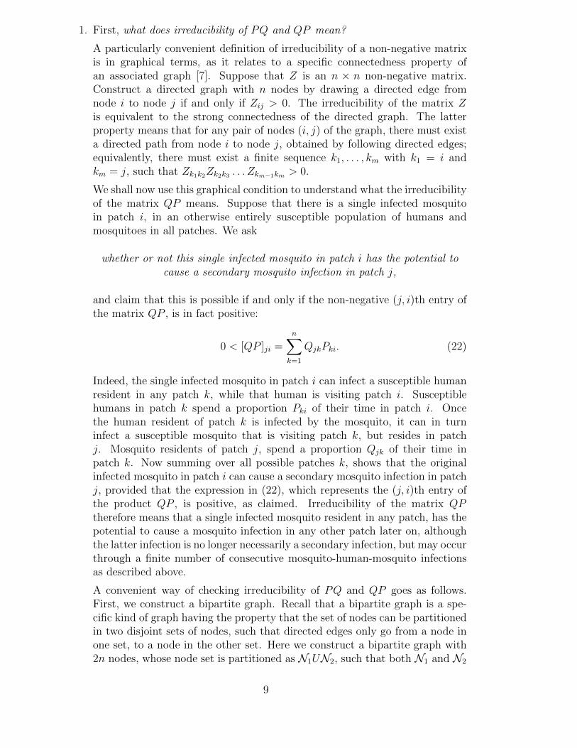
1. First, what does irreducibility of PQ and QP mean?

A particularly convenient definition of irreducibility of a non-negative matrixis in graphical terms, as it relates to a specific connectedness property ofan associated graph [7]. Suppose that Z is an n × n non-negative matrix.Construct a directed graph with n nodes by drawing a directed edge fromnode i to node j if and only if Zij > 0. The irreducibility of the matrix Zis equivalent to the strong connectedness of the directed graph. The latterproperty means that for any pair of nodes (i, j) of the graph, there must exista directed path from node i to node j, obtained by following directed edges;equivalently, there must exist a finite sequence k1, . . . , km with k1 = i andkm = j, such that Zk1k2Zk2k3 . . . Zkm−1km > 0.

We shall now use this graphical condition to understand what the irreducibilityof the matrix QP means. Suppose that there is a single infected mosquitoin patch i, in an otherwise entirely susceptible population of humans andmosquitoes in all patches. We ask

whether or not this single infected mosquito in patch i has the potential tocause a secondary mosquito infection in patch j,

and claim that this is possible if and only if the non-negative (j, i)th entry ofthe matrix QP , is in fact positive:

0 < [QP ]ji =n∑k=1

QjkPki. (22)

Indeed, the single infected mosquito in patch i can infect a susceptible humanresident in any patch k, while that human is visiting patch i. Susceptiblehumans in patch k spend a proportion Pki of their time in patch i. Oncethe human resident of patch k is infected by the mosquito, it can in turninfect a susceptible mosquito that is visiting patch k, but resides in patchj. Mosquito residents of patch j, spend a proportion Qjk of their time inpatch k. Now summing over all possible patches k, shows that the originalinfected mosquito in patch i can cause a secondary mosquito infection in patchj, provided that the expression in (22), which represents the (j, i)th entry ofthe product QP , is positive, as claimed. Irreducibility of the matrix QPtherefore means that a single infected mosquito resident in any patch, has thepotential to cause a mosquito infection in any other patch later on, althoughthe latter infection is no longer necessarily a secondary infection, but may occurthrough a finite number of consecutive mosquito-human-mosquito infectionsas described above.

A convenient way of checking irreducibility of PQ and QP goes as follows.First, we construct a bipartite graph. Recall that a bipartite graph is a spe-cific kind of graph having the property that the set of nodes can be partitionedin two disjoint sets of nodes, such that directed edges only go from a node inone set, to a node in the other set. Here we construct a bipartite graph with2n nodes, whose node set is partitioned as N1UN2, such that both N1 and N2

9

each have exactly n nodes. When Pij > 0 we draw a directed edge from theith node of N1, to the jth node of N2. Similarly, when Qkl > 0 we draw adirected edge from the kth node of N2, to the lth node of N1. This bipartitegraphs captures very well that the disease cannot be transmitted directly fromhost to host, or from vector to vector, but must go from vector to host, or fromhost to vector. One can think of the N1 as a representation of the n patches,from which weighted edges emanate that indicate the proportion of time, hu-mans spend among the patches (the entries of the matrix P ). Similarly, N2

represents the n patches, but now the weighted edges indicate the proportionof time mosquitoes spend among the patches (the entries of the matrix Q).We will “collapse” this bipartite graph in two distinct ways, ending up withtwo new directed graphs. These resulting graphs each have exactly n nodes,and irreducibility of QP and PQ will be equivalent to strong connectedness ofthese two graphs. Specifically, N1 is the node set of the first directed graph,and has a directed edge from node i to node j if [PQ]ij > 0, or equivalently ifthe bipartite graph has a directed path with exactly 2 edges, emanating fromthe ith node of N1, and ending in the jth node of N1. Of course, by the verynature of the bipartite graph, such a path must necessarily pass through somenode k belonging to N2. In a similar fashion, a second directed graph can beconstructed, but the node set of this second graph consists of the n nodes thatbelong to N2. Finally, irreducibility of PQ and QP is equivalent to the strongconnectedness of the two directed graphs we have just obtained.

This discussion concerning the irreducibility of PQ and QP also sheds light onthe reason why Theorem 2 establishes that if R(S) > 1, then the model has aunique, globally stable steady state with respect to which all non-zero solutionsconverge; this steady state represents a disease which is endemic in all patches,both for humans, as well as for mosquitoes. Indeed, for this to happen, theresult should hold if the initial condition corresponds to the presence of asingle infected mosquito, or a single infected human. In fact, these are typicalinitial conditions one encounters in practice. The discussion presented here, inconjunction with Theorem 2, shows that thanks to the irreducibility of bothPQ and QP , this single infected individual can indeed cause the disease tospread to the entire network for both populations, provided that R(S) > 1.

2. Note that irreducibility of P and Q does not imply irreducibility of their prod-ucts, as can be seen by the following simple example:

P =

(0 11 0

)= Q is irreducible, but PQ =

(1 00 1

)= QP is not.

Note also that (entry-wise) positivity of one of the matrices, is sufficient forirreducibility of the two products, because the product of a positive matrix,with a stochastic matrix is always positive.

On the other hand, irreducibility of both P and Q is not necessary for theirreducibility of PQ and QP . This is illustrated by two important special casesthat we consider in more detail later, namely when only humans move, butmosquitoes don’t, and vice versa. In this case, irreducibility of the mobility

10

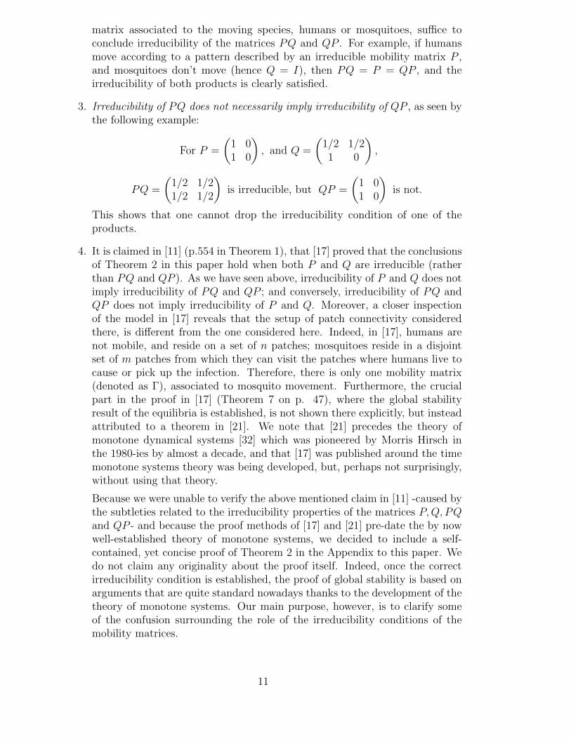
matrix associated to the moving species, humans or mosquitoes, suffice toconclude irreducibility of the matrices PQ and QP . For example, if humansmove according to a pattern described by an irreducible mobility matrix P ,and mosquitoes don’t move (hence Q = I), then PQ = P = QP , and theirreducibility of both products is clearly satisfied.

3. Irreducibility of PQ does not necessarily imply irreducibility of QP , as seen bythe following example:

For P =

(1 01 0

), and Q =

(1/2 1/21 0

),

PQ =

(1/2 1/21/2 1/2

)is irreducible, but QP =

(1 01 0

)is not.

This shows that one cannot drop the irreducibility condition of one of theproducts.

4. It is claimed in [11] (p.554 in Theorem 1), that [17] proved that the conclusionsof Theorem 2 in this paper hold when both P and Q are irreducible (ratherthan PQ and QP ). As we have seen above, irreducibility of P and Q does notimply irreducibility of PQ and QP ; and conversely, irreducibility of PQ andQP does not imply irreducibility of P and Q. Moreover, a closer inspectionof the model in [17] reveals that the setup of patch connectivity consideredthere, is different from the one considered here. Indeed, in [17], humans arenot mobile, and reside on a set of n patches; mosquitoes reside in a disjointset of m patches from which they can visit the patches where humans live tocause or pick up the infection. Therefore, there is only one mobility matrix(denoted as Γ), associated to mosquito movement. Furthermore, the crucialpart in the proof in [17] (Theorem 7 on p. 47), where the global stabilityresult of the equilibria is established, is not shown there explicitly, but insteadattributed to a theorem in [21]. We note that [21] precedes the theory ofmonotone dynamical systems [32] which was pioneered by Morris Hirsch inthe 1980-ies by almost a decade, and that [17] was published around the timemonotone systems theory was being developed, but, perhaps not surprisingly,without using that theory.

Because we were unable to verify the above mentioned claim in [11] -caused bythe subtleties related to the irreducibility properties of the matrices P,Q, PQand QP - and because the proof methods of [17] and [21] pre-date the by nowwell-established theory of monotone systems, we decided to include a self-contained, yet concise proof of Theorem 2 in the Appendix to this paper. Wedo not claim any originality about the proof itself. Indeed, once the correctirreducibility condition is established, the proof of global stability is based onarguments that are quite standard nowadays thanks to the development of thetheory of monotone systems. Our main purpose, however, is to clarify someof the confusion surrounding the role of the irreducibility conditions of themobility matrices.

11

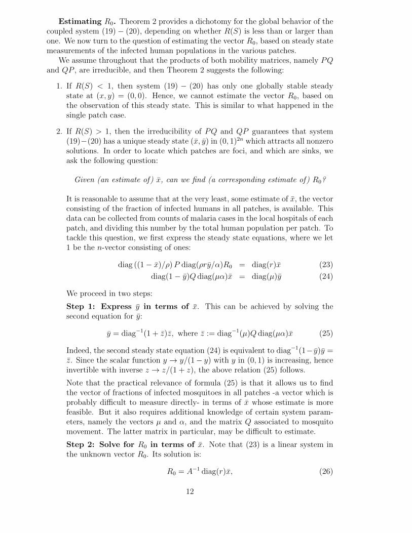
Estimating R0. Theorem 2 provides a dichotomy for the global behavior of thecoupled system (19)− (20), depending on whether R(S) is less than or larger thanone. We now turn to the question of estimating the vector R0, based on steady statemeasurements of the infected human populations in the various patches.

We assume throughout that the products of both mobility matrices, namely PQand QP , are irreducible, and then Theorem 2 suggests the following:

1. If R(S) < 1, then system (19) − (20) has only one globally stable steadystate at (x, y) = (0, 0). Hence, we cannot estimate the vector R0, based onthe observation of this steady state. This is similar to what happened in thesingle patch case.

2. If R(S) > 1, then the irreducibility of PQ and QP guarantees that system(19)−(20) has a unique steady state (x, y) in (0, 1)2n which attracts all nonzerosolutions. In order to locate which patches are foci, and which are sinks, weask the following question:

Given (an estimate of) x, can we find (a corresponding estimate of) R0?

It is reasonable to assume that at the very least, some estimate of x, the vectorconsisting of the fraction of infected humans in all patches, is available. Thisdata can be collected from counts of malaria cases in the local hospitals of eachpatch, and dividing this number by the total human population per patch. Totackle this question, we first express the steady state equations, where we let1 be the n-vector consisting of ones:

diag ((1− x)/ρ)P diag(ρry/α)R0 = diag(r)x (23)

diag(1− y)Q diag(µα)x = diag(µ)y (24)

We proceed in two steps:

Step 1: Express y in terms of x. This can be achieved by solving thesecond equation for y:

y = diag−1(1 + z)z, where z := diag−1(µ)Q diag(µα)x (25)

Indeed, the second steady state equation (24) is equivalent to diag−1(1− y)y =z. Since the scalar function y → y/(1− y) with y in (0, 1) is increasing, henceinvertible with inverse z → z/(1 + z), the above relation (25) follows.

Note that the practical relevance of formula (25) is that it allows us to findthe vector of fractions of infected mosquitoes in all patches -a vector which isprobably difficult to measure directly- in terms of x whose estimate is morefeasible. But it also requires additional knowledge of certain system param-eters, namely the vectors µ and α, and the matrix Q associated to mosquitomovement. The latter matrix in particular, may be difficult to estimate.

Step 2: Solve for R0 in terms of x. Note that (23) is a linear system inthe unknown vector R0. Its solution is:

R0 = A−1 diag(r)x, (26)

12

provided that the matrix:

A := diag ((1− x)/ρ)P diag(ρry/α), y given by (25),

is invertible.

Since (x, y) belongs to (0, 1)2n, invertibility of A is clearly equivalent to in-vertibility of P . Thus, if P is invertible, then (26) yields the vector of thebasic reproduction numbers of all the patches. In particular, we can then im-mediately read off which of the patches are sources, and which are sinks. Aninteresting situation arises when some of the patches in the network are sinks.Indeed, in this case, our method, allows us to estimate their basic reproductionnumber (assuming that the disease persists in the network), something whichwould have been impossible if these sinks were isolated patches as shown be-fore. One limitation of our method is that the matrix P should be invertible,and this may not always be the case, as

P =1

n

1 1 . . . 1...

... . . ....

1 1 . . . 1

shows. The structure of this matrix implies that humans of every patch dividetheir time equally among all patches.

Comments on estimating R0. Let us examine which model parameters, orparameter combinations, should be known in order to evaluate the right hand sideof (26), assuming that we have at least an estimate of x. From Step 1, we need thevectors µ and α, and the matrix Q, associated to mosquito movement. From Step2, we see that we also need the vector r, the vector ρ, and the matrix P , associatedto human mobility, and this matrix should be invertible.

In summary, we need the:

1. recovery rate vector r, and the death rate vector µ. 2

2. vector α, which consists of the probabilities that a susceptible mosquito be-comes infected over its entire lifetime, in all the patches.

3. the matrix P , which quantifies human movement.

4. the matrix Q, which quantifies mosquito movement.

5. vector ρ, consisting of the ratios of the total human populations in the variouspatches compared to the first patch.

6. the vector x, consisting of the proportions of human infected individuals inthe various patches.

2Actually, slightly less information is required. Indeed, it suffices that we know the ratios ofthe recovery rates, and the ratios of the death rates in the different patches. This follows from thefact that in (25) and in (26), there are factors diag(µ) and diag−1(µ), and diag(r) and diag−1(r)pre-and post-multiplying the matrix Q and P respectively.

13

Let us compare this to the traditional estimation method of R0, based on theoriginal definition (17), which provides formulas for its entries in terms of variousmodel parameters. This method requires for each patch i, the following information:

1. the recovery rate ri, the death rate µi.

2. the probability αi.

3. the biting rate ai.

4. the probability bi that an infectious mosquito bite successfully infects a sus-ceptible human.

5. the ratio of total number of mosquitoes and total number of humans mii =Vi/Hi.

6. the incubation period τi.

From both lists above, we see that the first two items of each method are thesame, but the next four are different.

The parameter which is perhaps the most difficult one to determine for ourestimation method (26) is Q, the mobility matrix associated to mosquito movement.This requires estimates of time spent by the mosquitoes among the various patches.On the other hand, in cases where the geographic scale of the patches is large,compared to typical distances traveled by mosquitoes, one may argue that Q = I.This expresses that mosquitoes are confined to their patch of residence. To a lesserextent, the mobility matrix P associated to human movement, may sometimes bedifficult to estimate, although mobile telephony data could be used for this purposeby tracking the movements of cell phone users.

The parameters which are the hardest to determine for the traditional method(17) are the ratios mii of the total number of mosquitoes over the total number ofhumans in each patch. Although the total number of humans in each patch is likelyto be well-known in many cases, this is far less likely in case of mosquitoes.

Finally, an important limitation of our method, compared to the traditional one,is that we require that R(S) > 1, so that the model has a positive steady state (x, y)in (0, 1)2n. In other words, our method requires the disease to be endemic, whereasthe traditional method also works when the disease is not endemic.

3 Bounds for R(S) and implications for control

In this Section we perform a closer examination of the spectral radius of the matrixS defined in (21), because the value of this spectral radius determines whether or notthe malaria infection persists in the patched network. We shall derive sharp upperand sharp lower bounds for this spectral radius in terms of the basic reproductionnumbers of all the patches, and the mobility matrices of vectors and hosts. Similarbounds have been obtained for various epidemic models of non-vector borne diseasesand using the Eulerian approach to model movement of individuals, see [18] for anSEIRP-model (P represents the class of partially immune individuals), [14] for an

14

SIS-model, and [4] for an SIR-model of a large metropolitan city and several satellitecities representing a suburban area.

Our analysis shall start with some special cases where either only humans move,or only mosquitoes. Later we turn to the general case where both move. We willsee that there are profound differences between the first two scenarios on the onehand, and the third one on the other.

A key technical property that we shall use repeatedly in this context, is that thespectral radius is a non-decreasing function over the set of non-negative matrices,i.e.:

0 ≤ A ≤ B ⇒ R(A) ≤ R(B). (27)

Here, the notation A ≤ B means that the entries of B are not smaller than thecorresponding entries of A. For a proof of this fact, see [7].

Below we use the notation xmin = mini(xi) and xmax = maxi(xi) for a givenvector x in Rn.

3.1 Only humans move

When only humans move it follows that the matrix associated to the mobility ofmosquitoes, is the identity matrix:

Q = I. (28)

In this case, the matrix S simplifies to the matrix Sh, which is defined as:

Sh = P diag(R0), (29)

and then we have the following bounds on the spectral radius of Sh:

Theorem 3. Assume that (28) and (29) hold. Then:

(R0)min ≤ R(Sh) ≤ (R0)max (30)

Moreover, these bounds are sharp in the sense that there exist row-stochastic matricesPmin and Pmax such that:

ρ (Pmin diag(R0)) = (R0)min and ρ (Pmax diag(R0)) = (R0)max (31)

Proof. Note that 0 ≤ Sh = P diag(R0) implies that:

0 ≤ (R0)minP ≤ Sh ≤ (R0)maxP,

and hence (30) follows from (27) and the fact that R(P ) = 1 (since P is row-stochastic). To prove that the lower bound is achieved, take Pmin as the matrixhaving exactly one column consisting of ones, namely the ith column where i isany index such that Ri

0 = (R0)min, and all other columns are zero vectors. Astraightforward calculation then shows that R(Pmin diag(R0)) = (R0)min. Similarly,to prove that the upper bound is achieved, set Pmax as the matrix having exactlyone column consisting of ones corresponding to an index j for which Rj

0 = (R0)max,and all other columns consisting of zero vectors. This proves (31).

15

From the point of view of malaria eradication in case only humans move, Theo-rem 3, in combination with Theorem 2, has several implications:

1. If all patches are foci, then the malaria infection will persist in the network,independently of network topology as encoded by the (human) mobility matrixP . Indeed, when all patches are transmission foci, then (R0)min > 1, andtherefore R(Sh) > 1 by (30). Theorem 2 then implies that the infectionpersists.

2. If all patches are sinks, then the malaria infection will be cleared from thenetwork, independently of network topology as encoded by the (human) mobilitymatrix P . Indeed, when all patches are sinks, then (R0)max < 1, and thereforeR(Sh) < 1 by (30). Theorem 2 then implies that the infection is cleared.

3. One control strategy is to identify all the foci (this can be achieved using theprocedure outlined in the previous Section), and make their corresponding basicreproduction number less than one by suitable local control measures, describedin the Section devoted to a single patch. This strategy is guaranteed to clearthe infection, independently of the network topology as encoded by the matrixP .

4. The latter control strategy is probably rather conservative because it is aimedat disease clearance for all network topologies. In practice, one is confrontedwith a specific topology, and it is conceivable that to clear the infection, notall foci should necessarily be made into sinks by appropriate local controlmeasures. To see that this can indeed happen, we consider a scenario with twopatches in which one patch is a source, and the other is a sink. Depending onthe network topology the infection may be cleared or may persist, highlightingthe crucial role played by the matrix P. Assume 2 patches such that

R0 =

(3/21/2

)In other words, patch 1 is a transmission focus, and patch 2 is a sink. Let

P1 =

(1/2 1/21/4 3/4

)and P2 =

(3/4 1/41/2 1/2

).

Then setting S1 = P1 diag(R0) and S2 = P2 diag(R0), we have that:

R(S1) ≈ 0.92 < 1, but R(S2) ≈ 1.22 > 1.

Thus, when human mobility is encoded by the matrix P1, the infection iscleared. But if it is encoded by P2, the infection persists.

5. Theorem 3 also suggests an alternative control strategy, namely to controlthe people’s mobility pattern by modifying the matrix P , for instance byprohibiting travel between certain patches. Indeed, the proof of Theorem 3shows that by making P equal to (or at least approximately equal to) thematrix Pmin, we can minimize R(Sh). The biological interpretation of Pmin is

16

that all humans should spend 100% of their time in the patch having lowestreproduction number, a result which makes sense intuitively.

Yet another control strategy can be gleaned from (30) in Theorem 3: Thestrategy which relocates people between patches in an appropriate way. Tosketch the main idea behind this strategy, consider for simplicity a scenariowith 2 patches where

R10 =

V1H1

a1b1α1 e−µ1τ1

r1and R2

0 =V2H2

a2b2α2 e−µ2τ1

r2

and such thatR1

0 < 1 < R20.

Consequently, (R0)max = R20 > 1, and therefore the infection will persist in

the two-patch system, at least for some human mobility matrices P . Con-trol strategies based on relocation only, amount to keeping all parametersVi, ai, bi, αi, µi, τi and ri fixed for i = 1, 2, but allowing H1 and H2 to vary,as long as their sum remains constant. In this particular case, to clear theinfection, we would seek to decrease R2

0 below 1, while maintaining R10 below

1 as well. This may be achieved by increasing H2 and decreasing H1 by anequal amount. In practice, this means that human individuals would be relo-cated from patch 1 to patch 2. The difficulty lies in the fact that although wecan obviously always make R2

0 less than 1 by an appropriate decrease in H2,the corresponding increase in H1 might push R1

0 above 1, in which case therelocation strategy will fail to clear the infection.

3.2 Only mosquitoes move

In this case, the matrix P associated to human movement, is the identity matrix:

P = I. (32)

The matrix S simplifies to the matrix Sm which is defined as:

Sm = diag(R0)D−1QD, (33)

and then spectral radius of Sm is bounded as follows:

Theorem 4. Assume that (32) and (33) hold. Then:

(R0)min ≤ R(Sm) ≤ (R0)max (34)

Moreover, these bounds are sharp in the sense that there exist row-stochastic matricesQmin and Qmax such that:

ρ(diag(R0)D

−1QminD)

= (R0)min and ρ(diag(R0)D

−1QmaxD)

= (R0)max (35)

Proof. Since R(AB) = R(BA) for any square matrices A and D, it follows thatR(Sm) = R (diag(R0)DD

−1Q) = R (Q diag(R0)), and then the rest of the proof issimilar to that of Theorem 3.

17

All the remarks we made concerning disease control in case only humans move,remain valid here as well: simply replace the matrix P by the matrix Q in thediscussion following Theorem 3. In particular, when all patches are focal areas, thedisease persists, and when all patches are sinks, the disease is cleared, independentof the network topology associated to the mosquito movement matrix Q. Hence, aconservative control strategy is to make the reproduction numbers of all patches lessthen one, using local control measures described in the Section devoted to a singlepatch. When some patches are transmission foci but others are sinks, there existmosquito mobility matricesQ which give rise to disease persistence, but also matricesQ giving rise to disease clearance. Finally, another possible control strategy, is toredistribute mosquitoes between various patches, similarly to the relocation strategyof humans described in the previous subsection. In practice this can be achieved byplacing repellants in patches with high basic reproduction values, effectively reducingthe total number of mosquitoes V in those patches. However, these mosquitoes willmove to other patches, where they in turn will increase the basic reproductionnumber. The failure or success of this strategy depends on whether or not thereplaced mosquitoes push the basic reproduction values in their new home patchesabove 1.

3.3 Both humans and mosquitoes move

This is the general case, where both P and Q are assumed to differ from the identitymatrix. First, we define the positive vector d as:

d = (ac)/(rρ).

Note that this implies that the diagonal matrix D in (21) contains the componentsof d on its diagonal: D = diag(d), and hence (21) can be re-written as:

S = P diag(R0/d)Q diag(d) (36)

Then we have:

Theorem 5. The spectral radius of S is bounded as follows:

dmin(R0/d)min ≤ R(S) ≤ dmax(R0/d)max (37)

Moreover, these bounds are sharp in the sense that there exist pairs of row-stochasticmatrices (Pmin, Qmin) and (Pmax, Qmax) such that:

ρ (Pmin diag(R0/d)Qmin diag(d)) = dmin(R0/d)min, and (38)

ρ (Pmax diag(R0/d)Qmax diag(d)) = dmax(R0/d)max. (39)

Proof. From (36) follows that:

dmin(R0/d)minPQ ≤ S ≤ dmax(R0/d)maxPQ,

and therefore, upon taking the spectral radius of the matrices above, the fact thatR(PQ) = 1 (because the product of two row-stochastic matrices is row-stochastic,

18

hence has spectral radius 1), (27) implies (37). To prove (38) and (39) we use asimilar argument as in the proof of Theorem 3. For instance, to prove (38) wecan take Pmin to be a matrix having exactly one column consisting of ones, namelythe ith column corresponding to the minimal component of the vector R0/d, andall other columns are zero vectors. Similarly for Qmin we take a matrix havingexactly one column consisting of ones, namely the jth column corresponding to theminimal component of the vector d, and all other columns are zero vectors. Then astraightforward calculation shows that (38) holds.

Although many of the remarks we made concerning disease control following The-orem 3 and Theorem 4, remain valid in the case that both humans and mosquitoesmove, we point out some striking differences:

1. The conservative control strategy that made the basic reproduction numbers inall patches less than one using local control measures, no longer guarantees thatthe disease will be cleared from the network, independently of the movementmatrices P and Q. Indeed, although this strategy ensures that (R0)max < 1,it does not necessarily make dmax(R0/d)max < 1. For example, in a 2 patchsystem with:

R0 =

(1/21/4

)and d =

(1/41

)there holds that:

1/2 = (R0)max < 1 < dmax(R0/d)max = max ((1/2)/(1/4), 1/4) = 2.

Consequently, Theorem 5 also says that there are in fact network topologiesfor human (P ) and mosquito (Q) movement , such that the disease persists(because the upper bound for R(S), which is 2, can be achieved), despite thefact that (R0)max < 1. In other words, contrary to what happened in thecases where only humans or only mosquito move, the disease may persist in anetwork of sinks.

2. Similar arguments show that when both humans and mosquitoes move, it ispossible that the disease is cleared from a network of sources. This contraststhe cases where either only humans, or only mosquitoes move. For instance,when

R0 =

(24

)and d =

(1

1/4

)then

1/2 = (1/4) min(2, 16) = dmin(R0/d)min < 1 < (R0)min = 2.

The two examples above, indicate that knowledge of the maximal and minimalcomponent of the vector R0, i.e. the maximal and minimal basic reproductionnumber of all the patches in isolation, is no longer sufficient to predict diseaseclearance or persistence from the network. Instead, according to the bounds (37) inTheorem 5, the product of the maximal and minimal components of the vectors dand R0/d are the relevant quantities. Therefore, control strategies focused on thebasic reproduction numbers of isolated patches, are no longer adequate when bothhosts and vectors move. From a practical control perspective, this may be the mostimportant conclusion of the mathematical analysis presented here.

19

4 Conclusion

Robust strategies for malaria elimination that account for parasite movement arecritical for malaria control programs [25], and strategies that spatially target vectorcontrol and treatment will improve the efficiency of the use of limited resources.Being able to predict how control will affect parasite populations across networks ofpatches has been characterized statistically, but it also requires a mechanistic un-derstanding of transmission and parasite mobility, as mediated by both mosquitoesand humans. However, most algorithms for quantifying transmission intensity acrossheterogeneous landscape either do not incorporate mobility in both hosts [29, 38] orare purely statistical identification methods [8]. In the multi-patch Ross-Macdonaldmodel we analyzed to identify patches that are transmission foci, which incorporatesboth human and mosquito movement, we test whether targeting foci based on localestimates of transmission is a viable strategy for eliminating parasite populationsregionally. We find that while this strategy is sufficient to eliminate all parasites ifonly humans or mosquitoes move, when both hosts move, there are network topolo-gies that can cause a strategy that only targets foci to fail. This result highlightsthe complex interactions between malaria parasite, human, and mosquito popula-tions caused by host mobility, and the need for understanding the specific movementpatterns of humans and mosquitoes when developing malaria elimination strategies.More generally, it is well-known that the basic reproduction number R0 plays animportant role in various models of the spread of many infectious diseases, yet con-trol measures aimed at simply reducing R0 below 1 may be insufficient to clear theinfection. Our results are in accordance with that observation.

We conclude with some comments related to the practical use of our results. Anontrivial problem when using the proposed patched Ross-Macdonald model, is todefine the various patches in the system. Policy makers who would use this model intheir decision process, will have to identify the various patches first, before they canimplement specific control strategies. Obviously, there is no unique way to do this.For example, a lot depends on the geographic scale of the infection dynamics: thiscould range from systems of nearby towns that are connected via small trails or pavedroads for humans, and rivers or lakes for mosquitoes, over counties to provinces andcountries, or even on a global scale by transport via boats and air. This variability ingeographic scale also affects judicious choices of the mobility matrices needed in ourmodel: people travel far less frequently via air to other countries, than they do tothe local fitness club two towns over. There is nothing singular about the problem ofchoosing patches in the context of the patched Ross-Macdonald model investigatedhere. In fact, users of any patch model face this issue as well. Nevertheless, webelieve that they constitute a good first step towards a better understanding ofmore complicated models that incorporate spatial features more explicitly, such aspartial differential equations models.

20

Appendices

A Quasi-monotone matrices and monotone sys-

tems

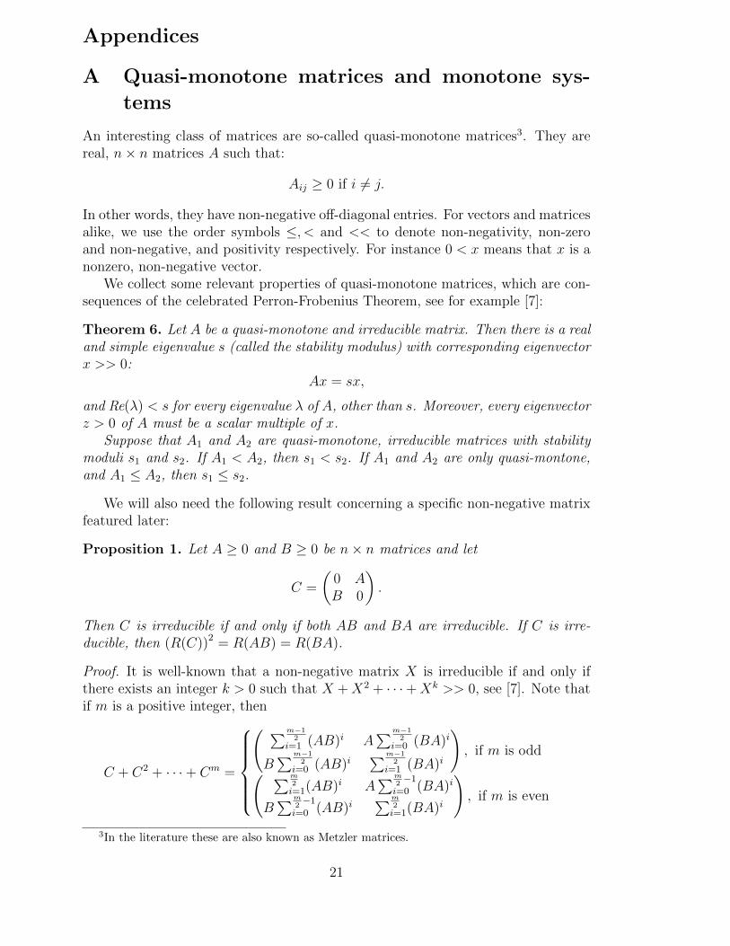
An interesting class of matrices are so-called quasi-monotone matrices3. They arereal, n× n matrices A such that:

Aij ≥ 0 if i 6= j.

In other words, they have non-negative off-diagonal entries. For vectors and matricesalike, we use the order symbols ≤, < and << to denote non-negativity, non-zeroand non-negative, and positivity respectively. For instance 0 < x means that x is anonzero, non-negative vector.

We collect some relevant properties of quasi-monotone matrices, which are con-sequences of the celebrated Perron-Frobenius Theorem, see for example [7]:

Theorem 6. Let A be a quasi-monotone and irreducible matrix. Then there is a realand simple eigenvalue s (called the stability modulus) with corresponding eigenvectorx >> 0:

Ax = sx,

and Re(λ) < s for every eigenvalue λ of A, other than s. Moreover, every eigenvectorz > 0 of A must be a scalar multiple of x.

Suppose that A1 and A2 are quasi-monotone, irreducible matrices with stabilitymoduli s1 and s2. If A1 < A2, then s1 < s2. If A1 and A2 are only quasi-montone,and A1 ≤ A2, then s1 ≤ s2.

We will also need the following result concerning a specific non-negative matrixfeatured later:

Proposition 1. Let A ≥ 0 and B ≥ 0 be n× n matrices and let

C =

(0 AB 0

).

Then C is irreducible if and only if both AB and BA are irreducible. If C is irre-ducible, then (R(C))2 = R(AB) = R(BA).

Proof. It is well-known that a non-negative matrix X is irreducible if and only ifthere exists an integer k > 0 such that X +X2 + · · ·+Xk >> 0, see [7]. Note thatif m is a positive integer, then

C + C2 + · · ·+ Cm =

( ∑m−12

i=1 (AB)i A∑m−1

2i=0 (BA)i

B∑m−1

2i=0 (AB)i

∑m−12

i=1 (BA)i

), if m is odd( ∑m

2i=1(AB)i A

∑m2−1

i=0 (BA)i

B∑m

2−1

i=0 (AB)i∑m

2i=1(BA)i

), if m is even

3In the literature these are also known as Metzler matrices.

21

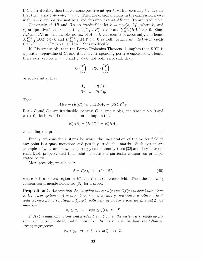
If C is irreducible, then there is some positive integer k, with necessarily k > 1, suchthat the matrix C+· · ·+Ck >> 0. Then the diagonal blocks in the expression abovewith m = k are positive matrices, and this implies that AB and BA are irreducible.

Conversely, if AB and BA are irreducible, let k = max(k1, k2), where k1 andk2 are positive integers such that

∑k1i=1(AB)i >> 0 and

∑k2i=1(BA)i >> 0. Since

AB and BA are irreducible, no row of A or B can consist of zeros only, and henceA∑k

i=1(BA)i >> 0 and B∑k

i=1(AB)i >> 0 as well. Setting m = 2(k + 1) yieldsthat C + · · ·+ Cm >> 0, and then C is irreducible.

If C is irreducible, then the Perron-Frobenius Theorem [7] implies that R(C) isa positive eigenvalue of C, and it has a corresponding positive eigenvector. Hence,there exist vectors x >> 0 and y >> 0, not both zero, such that:

C

(xy

)= R(C)

(xy

),

or equivalently, that

Ay = R(C)x

Bx = R(C)y

ThenABx = (R(C))2 x and BAy = (R(C))2 y.

But AB and BA are irreducible (because C is irreducible), and since x >> 0 andy >> 0, the Perron-Frobenius Theorem implies that

R(AB) = (R(C))2 = R(BA),

concluding the proof.

Finally, we consider systems for which the linearization of the vector field inany point is a quasi-monotone and possibly irreducible matrix. Such system areexamples of what are known as (strongly) monotone systems [32] and they have theremarkable property that their solutions satisfy a particular comparison principlestated below.

More precisely, we consider

x = f(x), x ∈ U ⊂ Rn, (40)

where U is a convex region in Rn and f is a C1 vector field. Then the followingcomparison principle holds, see [32] for a proof:

Proposition 2. Assume that the Jacobian matrix J(x) := Df(x) is quasi-monotonein U . Then system (40) is monotone, i.e. if x0 and y0 are initial conditions in Uwith corresponding solutions x(t), y(t) both defined on some positive interval I, wehave that:

x0 ≤ y0 ⇒ x(t) ≤ y(t), t ∈ I.If J(x) is quasi-monotone and irreducible in U , then the system is strongly mono-

tone, i.e. it is monotone, and for initial conditions x0 ≤ y0, we have the followingstronger property:

x0 < y0 ⇒ x(t) << y(t), t ∈ I.

22

B Proof of the dychotomy

Proof of Theorem 2. System (19) − (20) is strongly monotone on [0, 1)2n byProposition 2. Indeed, the Jacobian matrix is:

J(x, y) =

(−D1(y) diag(1− x) diag−1(ρ)P diag(ρR0r/α)

diag(1− y)Q diag(µα) −D2(x)

),

where D1(y) and D2(x) are positive diagonal matrices whose diagonal entries dependonly on the indicated arguments y and x respectively. As long as all xi and all yi arenot equal to 1, J(x, y) is a quasi-monotone and irreducible matrix. (irreducibilityfollows from Proposition 1 because PQ and QP are irreducible, and because nocomponent of x or y equals 1) Consequently, the system is strongly monotone inthis region of the state space.

Nonzero solutions starting on the boundary of [0, 1]2n enter (0, 1)2n instanta-neously (when xi = 1 or yi = 1 this is immediate; and when xi = 0 or yi = 0, thisfollows because the flow is strongly monotone on [0, 1)2n and because (x, y) = (0, 0)is a steady state). In particular, the only steady state on the boundary of [0, 1]2n isthe zero steady state (x, y) = (0, 0).

Next we consider the local stability properties of the zero steady state (0, 0).These are determined by the location of eigenvalues of J(0, 0) in the complex plane.Since D1(0) = diag(r) and D2(0) = diag(µ), we have that:

J(0, 0) =

(− diag(r) diag−1(ρ)P diag(ρR0r/α)Q diag(µα) − diag(µ)

)Following [13] we rewrite this matrix as the difference of a non-negative matrix Fand a nonsingular M-matrix V as follows:

J(0, 0) = F − V,

where

F =

(0 diag−1(ρ)P diag(ρR0r/α)

Q diag(µα) 0

), and V =

(diag(r) 0

0 diag(µ)

).

Let s denote the stability modulus of J(0, 0). The proof of the Theorem 2 in [13]shows that:

s

< 0

= 0

> 0

if and only if R(FV −1)

< 1

= 1

> 1

(41)

Consequently, the local stability properties of the steady state (0, 0) which are de-termined by the sign of s, can be equivalently derived from the spectral radius ofthe matrix FV −1:

FV −1 =

(0 diag−1(ρ)P diag ((ρR0r)/(αµ))

Q diag(αµ/r) 0

).

23

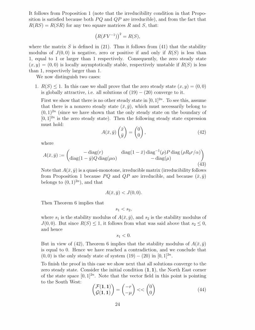
It follows from Proposition 1 (note that the irreducibility condition in that Propo-sition is satisfied because both PQ and QP are irreducible), and from the fact thatR(RS) = R(SR) for any two square matrices R and S, that:(

R(FV −1))2

= R(S),

where the matrix S is defined in (21). Thus it follows from (41) that the stabilitymodulus of J(0, 0) is negative, zero or positive if and only if R(S) is less than1, equal to 1 or larger than 1 respectively. Consequently, the zero steady state(x, y) = (0, 0) is locally asymptotically stable, respectively unstable if R(S) is lessthan 1, respectively larger than 1.

We now distinguish two cases:

1. R(S) ≤ 1. In this case we shall prove that the zero steady state (x, y) = (0, 0)is globally attractive, i.e. all solutions of (19)− (20) converge to it.

First we show that there is no other steady state in [0, 1]2n. To see this, assumethat there is a nonzero steady state (x, y), which must necessarily belong to(0, 1)2n (since we have shown that the only steady state on the boundary of[0, 1]2n is the zero steady state). Then the following steady state expressionmust hold:

A(x, y)

(xy

)=

(00

), (42)

where

A(x, y) :=

(− diag(r) diag(1− x) diag−1(ρ)P diag (ρR0r/α)

diag(1− y)Q diag(µα) − diag(µ)

)(43)

Note thatA(x, y) is a quasi-monotone, irreducible matrix (irreducibility followsfrom Proposition 1 because PQ and QP are irreducible, and because (x, y)belongs to (0, 1)2n), and that

A(x, y) < J(0, 0).

Then Theorem 6 implies thats1 < s2,

where s1 is the stability modulus of A(x, y), and s2 is the stability modulus ofJ(0, 0). But since R(S) ≤ 1, it follows from what was said above that s2 ≤ 0,and hence

s1 < 0.

But in view of (42), Theorem 6 implies that the stability modulus of A(x, y)is equal to 0. Hence we have reached a contradiction, and we conclude that(0, 0) is the only steady state of system (19)− (20) in [0, 1]2n.

To finish the proof in this case we show next that all solutions converge to thezero steady state. Consider the initial condition (1,1), the North East cornerof the state space [0, 1]2n. Note that the vector field in this point is pointingto the South West: (

F(1,1)G(1,1)

)=

(−r−µ

)<<

(00

)(44)

24

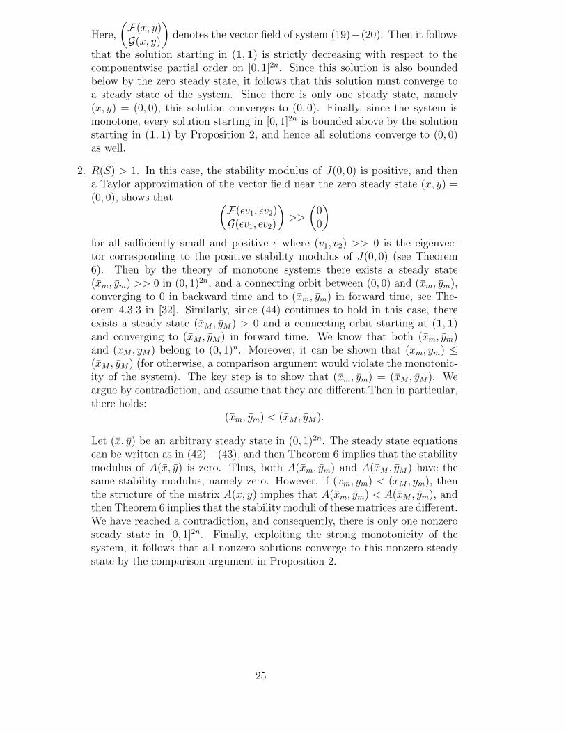
Here,

(F(x, y)G(x, y)

)denotes the vector field of system (19)−(20). Then it follows

that the solution starting in (1,1) is strictly decreasing with respect to thecomponentwise partial order on [0, 1]2n. Since this solution is also boundedbelow by the zero steady state, it follows that this solution must converge toa steady state of the system. Since there is only one steady state, namely(x, y) = (0, 0), this solution converges to (0, 0). Finally, since the system ismonotone, every solution starting in [0, 1]2n is bounded above by the solutionstarting in (1,1) by Proposition 2, and hence all solutions converge to (0, 0)as well.

2. R(S) > 1. In this case, the stability modulus of J(0, 0) is positive, and thena Taylor approximation of the vector field near the zero steady state (x, y) =(0, 0), shows that (

F(εv1, εv2)G(εv1, εv2)

)>>

(00

)for all sufficiently small and positive ε where (v1, v2) >> 0 is the eigenvec-tor corresponding to the positive stability modulus of J(0, 0) (see Theorem6). Then by the theory of monotone systems there exists a steady state(xm, ym) >> 0 in (0, 1)2n, and a connecting orbit between (0, 0) and (xm, ym),converging to 0 in backward time and to (xm, ym) in forward time, see The-orem 4.3.3 in [32]. Similarly, since (44) continues to hold in this case, thereexists a steady state (xM , yM) > 0 and a connecting orbit starting at (1,1)and converging to (xM , yM) in forward time. We know that both (xm, ym)and (xM , yM) belong to (0, 1)n. Moreover, it can be shown that (xm, ym) ≤(xM , yM) (for otherwise, a comparison argument would violate the monotonic-ity of the system). The key step is to show that (xm, ym) = (xM , yM). Weargue by contradiction, and assume that they are different.Then in particular,there holds:

(xm, ym) < (xM , yM).

Let (x, y) be an arbitrary steady state in (0, 1)2n. The steady state equationscan be written as in (42)− (43), and then Theorem 6 implies that the stabilitymodulus of A(x, y) is zero. Thus, both A(xm, ym) and A(xM , yM) have thesame stability modulus, namely zero. However, if (xm, ym) < (xM , ym), thenthe structure of the matrix A(x, y) implies that A(xm, ym) < A(xM , ym), andthen Theorem 6 implies that the stability moduli of these matrices are different.We have reached a contradiction, and consequently, there is only one nonzerosteady state in [0, 1]2n. Finally, exploiting the strong monotonicity of thesystem, it follows that all nonzero solutions converge to this nonzero steadystate by the comparison argument in Proposition 2.

25

References

[1] Arino, J., and van den Driessche, P., A multi-city epidemic model, Mathemat-ical Population Studies 10, 175-193, 2003.

[2] Arino, J., Davis, J.R., Hartley, D., Jordan, R., Miller, J.M., and van denDriessche, P., A multi-species epidemic model with spatial dynamics, Mathe-matical Medicine and Biology 22, 129-142, 2005.

[3] Arino, J., Diseases in metapopulations, In: Ma, Z., Zhou, Y., and Wu, J.,Eds., Modeling and Dynamics of Infectious Diseases, 65-123, World Scientific,2009.

[4] Arino, J., and Portet, S., Epidemiological implications of mobility between alarge urban centre and smaller satellite cities, Journal of Mathematical Biology71, 1243-1265, 2015.

[5] Auger, P., Kouokam, E., Sallet, G., Tchuente, M., and Tsanou, B., The Ross-Macdonald model in a patchy environment, Mathematical Biosciences 216,123-131, 2008.

[6] Bejon, P., Williams, T.N., Nyundo,C., Hay, S.I., Benz, D., Gething,P.W.,Otiende, M., Peshu, J., Bashraheil,M., Greenhouse,B., Bousema, T., Bauni,E., Marsh,K., Smith, D.L., and Borrmann, S., A micro-epidemiological analy-sis of febrile malaria in Coastal Kenya showing hotspots within hotspots. eLife1-19, doi:10.7554/eLife.02130, 2014.

[7] Berman, A., and Plemmons, P.J., Nonnegative Matrices in the MathematicalSciences, SIAM, 1994.

[8] Bousema, T., Drakeley, C., Gesase, S., Hashim, R., Magesa, S., Mosha, F.,Otieno, S., Carneiro, I., Cox, J., Msuya, E., Kleinschmidt, I., Maxwell, C.,Greenwood, B., Riley, E., Sauerwein, R., Chandramohan, D., and Gosling,R., Identification of hot spots of malaria transmission for targeted malariacontrol, Journal of Infectious Diseases 201, 1764-1774, 2010.

[9] Bousema, T., Griffin, J.T., Sauerwein, R.W., Smith, D.L., Churcher, T.S.,Takken, W., Ghani, A., Drakeley, C., and Gosling, R., Hitting hotspots:Spatial targeting of malaria for control and elimination, PLOS Medicine 9,e1001165, 2012.

[10] http://www.cdc.gov/malaria/about/faqs.html

[11] Cosner, C., Beier, J.C., Cantrell, R.S., Impoinvil, D., Kapitanski, L., PottsM.D., Troyo, A., and Ruan, S., The effects of human movement on the per-sistence of vector-borne diseases, Journal of Theoretical Biology 258, 550-560,2009.

[12] Cosner, C., Models for the effects of host movement in vector-borne diseasesystems, Mathematical Biosciences 270, 192-197, 2015.

26

[13] van den Driessche, P., and Watmough, J. Reproduction numbers and sub-threshold endemic equilibria for compartmental models of disease transmis-sion, Mathematical Biosciences 180, 29-48, 2002.

[14] Gao, D., and Ruan, S., An SIS patch model with variable transmission coeffi-cients, Mathematical Biosciences 232, 110-115, 2011.

[15] Gao, D., and Ruan, S., Malaria models with spatial effects, In: Chen, D.,Moulin, B., and Wu, J., Eds., Analyzing and Modeling Spatial and TemporalDynamics of Infectious Diseases, 3-30, John Wiley & Sons, 2014.

[16] Githeko, A.K., Ayisi, J.M., Odada, P.K., Atieli, F.K., Ndenga, B.A., Githure,J.I., and Yan, G., Topography and malaria transmission heterogeneity in west-ern Kenya highlands: prospects for focal vector control, Malaria Journal 5,107, 2006.

[17] Hasibeder, G., and Dye, C., Population dynamics of mosquito-borne disease:persistence in a completely heterogeneous environment, Theoretical Popula-tion Biology 33, 31-53, 1988.

[18] Hsieh, Y.-H., van den Driessche, P., and Wang, L., Impact of Travel BetweenPatches for Spatial Spread of Disease, Bulletin of Mathematical Biology 69,1355-1375, 2007.

[19] Killeen, G.F., Knols, B.G.J., and Gu, W., Taking malaria transmission out ofthe bottle: implications of mosquito dispersal for vector-control interventions,Lancet Infectious Diseases 3, 297-303, 2003.

[20] Koella, J.C., On the use of mathematical models of malaria transmission, ActaTropica 49, 1-25, 1991.

[21] Lajmanovich, A., Yorke, J.A., A deterministic model for gonorrhea in a non-homogeneous population. Mathematical Biosciences 28, 221-236, 1976.

[22] Li, C.-K., and Schneider, H., Journal of Mathematical Biology 44, 450-462,2002.

[23] Manore, C.A., Hickmann, K.S., Hyman, J.M., Foppa, I.M., Davis, J.K., Wes-son, D.M., and Mores, C.N., A network-patch methodology for adaptingagent-based models for directly transmitted disease to mosquito-borne dis-ease, arXiv:1405.2258v1.

[24] Mbogo, C.M., Mwangangi, J.M., Nzovu, J., Gu, W., Yan, G., Gunter, J.T.,Swalm, C., Keating, J., Regens, J.L., Shililu, J.I., Githure, J.I., and Beier,J.C., Spatial and temporal heterogeneity of Anopheles mosquitoes and Plas-modium falciparum transmission along the Kenyan coast, American Journalof Tropical Medicine and Hygiene 68, 734-742, 2003.

[25] Moonen, B., Cohen, J.M., Snow, R.W., Slutsker, L., Drakeley, C., Smith, D.L.,Abeyasinghe R.R., Rodriguez, M.H., Maharaj, R., Tanner, M., and Targett,G., Operation strategies to achieve and maintain malaria elimination, Lancet376, 1692-1603, 2010.

27

[26] Ruktanonchai, N.W., De Leenheer, P., Tatem, A.J., Alegana, V.A., Caugh-lin, T.T., zu Erbach-Schoenberg, E. , Loureno, C., Ruktanonchai, C.W.,and Smith, D.L., Identifying Malaria Transmission Foci for Elimination Us-ing Human Mobility Data, PLOS Computational Biology 12(4): e1004846.doi:10.1371/journal. pcbi.1004846.

[27] Paull, S.H., Song, S., McClure, K.M., Sackett, L.C., Kilpatrick A.M., andJohnson, P.T.J., From superspreaders to disease hotspots: linking transmis-sion across hosts and space, Frontiers of Ecology and Environment 10, 75-82,2012.

[28] Prothero, R.M., Disease and mobility: a neglected factor in epidemiology,International Journal of Epidemiology 6, 259-267, 1977.

[29] Prosper, O., Ruktanonchai, N., and Martcheva, M., Assessing the role of spa-tial heterogeneity and human movement in malaria dynamics and control,Journal of Theoretical Biology 303, 1-14, 2012.

[30] Rodriguez, D.J., and Torres-Sorando, L., Models of infectious diseases in spa-tially heterogeneous environments, Bulletin of Mathematical Biology 63, 547-571, 2001.

[31] Ruktanonchai, N.W., De Leenheer, P., Tatem, A.J., Alegana, V.A., Caugh-lin, T.T., zu Erbach-Schoenberg, E., Lourenco, C., Ruktanonchai, C.W., andSmith, D.L., Identifying Malaria Transmission Foci for Elimination Using Hu-man Mobility Data. PLoS Comput Biol 12(4): e1004846. doi:10.1371/journal.pcbi.1004846.

[32] Smith, H.L., Monotone Dynamical Systems, AMS, 1995.

[33] Smith, D.L., and McKenzie, F.E., Statics and dynamics of malaria infectionin Anopheles mosquitoes, Malaria Journal 3,13, 2004.

[34] Smith, D.L., Battle, K.E., Hay, S.I., Barker, C.M., Scott, T.W., and McKen-zie, F.E., Ross, Macdonald, and a Theory for the Dynamics and Control ofMosquito-Transmitted Pathogens, PLoS Pathogens 8, e1002588, 2012.

[35] Stoddard, S.T., Morrison, A.C., Vazquez-Prokopec, G.M., Soldan V.P.,Kochel, T.J., Kitron, U., Elder, J.P., and Scott, T.W., The role of humanmovement in the transmission of vector-borne pathogens, PLOS NeglectedTropical Diseases 3, e481, 2009.

[36] Tatem, A.J., and Smith, D.L., International population movements and re-gional Plasmodium falciparum malaria elimination strategies, Proceedings ofthe National Academy of Sciences 107, 12222-12227, 2010.

[37] Wang, W., Epidemic models with population dispersal, In: Takeuchi,Y.,Iwasa,Y., and Sato, K., Eds., Mathematics for Life Science and Medicine,67-95, Springer-Verlag, 2007.

28

[38] Wesolowski A., Eagle, N., Tatem, A.J., Smith, D.L., Noor, A.M., Snow, R.W.,and Buckee C.O., Quantifying the impact of human mobility on malaria, Sci-ence 338, 267-270, 2012.

[39] Zhuo, G., Munga, S., Minakawa, N., Githeko, A.K., and Yan, G., Spatial rela-tionship between adult malaria vector abundance and environmental factors inwestern Kenya highlands, American Journal of Tropical Medicine and Hygiene77, 29-35, 2007.

29