Parametric Signal Processing

Shu NamikiNational Institute of Advanced Industrial Science and Technology (AIST)

Network Photonics Research Center

Part of this work is supported by - Project for Developing Innovation Systems of the Ministry of Education, Culture,

Sports, Science and Technology (MEXT), Japan.

ECOC, 21 Sept. 2014WS2 - WHAT IS THE ROLE OF OPTICAL SIGNAL PROCESSING IN THE AGE OF DSP?

1

OSP vs DSP.. Nothing is trans-historical.., but fundamental physics.

• The old wisdom says, “Don’t fight with silicon!”– Digital coherent has obviated many of our good ol’ “cool” optical signal

processing topics at least in the 100G generation..– But, silicon is finally having difficulty in further scaling..

• How can optical signal processing be compelling to help silicon?– Be compatible with digital coherent signals– Help off-load DSPs and lower the entire cost– Be superior to O/E:E/O alternatives– Be capable of completely new functions

2 S. Namiki, ECOC2014, WS2, Cannes

Disp. Comp.

FEC

Others DBP＋

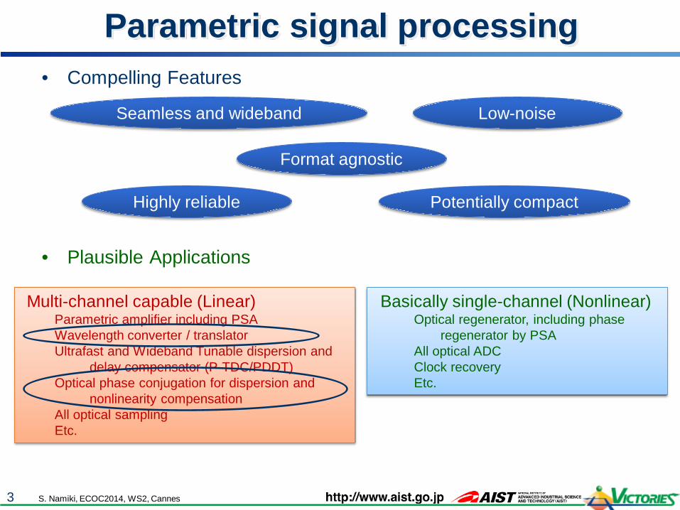
Parametric signal processing• Compelling Features

• Plausible Applications

3 S. Namiki, ECOC2014, WS2, Cannes

Format agnostic

Low-noiseSeamless and wideband

Highly reliable Potentially compact

Multi-channel capable (Linear)Parametric amplifier including PSAWavelength converter / translatorUltrafast and Wideband Tunable dispersion and

delay compensator (P-TDC/PDDT)Optical phase conjugation for dispersion and

nonlinearity compensationAll optical samplingEtc.

Basically single-channel (Nonlinear)Optical regenerator, including phase

regenerator by PSAAll optical ADCClock recoveryEtc.

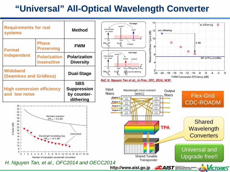
“Universal” All-Optical Wavelength Converter

Requirements for real systems Method

Format Independent

Phase Preserving FWM

Polarization Insensitive

PolarizationDiversity

Wideband(Seamless and Gridless) Dual-Stage

High conversion efficiency and low noise

SBS Suppressionby counter-

dithering

Ref: H. Nguyen Tan et al., in Proc. OFC, 2014, W3F.

Shared TunableTransponder

Degree 1

Degree 2

Degree 3

Degree 4

Wavelength cross connect(WXC)

WSS/Splitter

WSS/Coupler

WSS/Splitter

WSS/Splitter

WSS/Splitter

WSS/Coupler

WSS/Coupler

WSS/Coupler

Input fibers

Output fibers

TPAShared

Wavelength Converters

Flex-GridCDC-ROADM

Universal and Upgrade free!!

H. Nguyen Tan, et al., OFC2014 and OECC2014

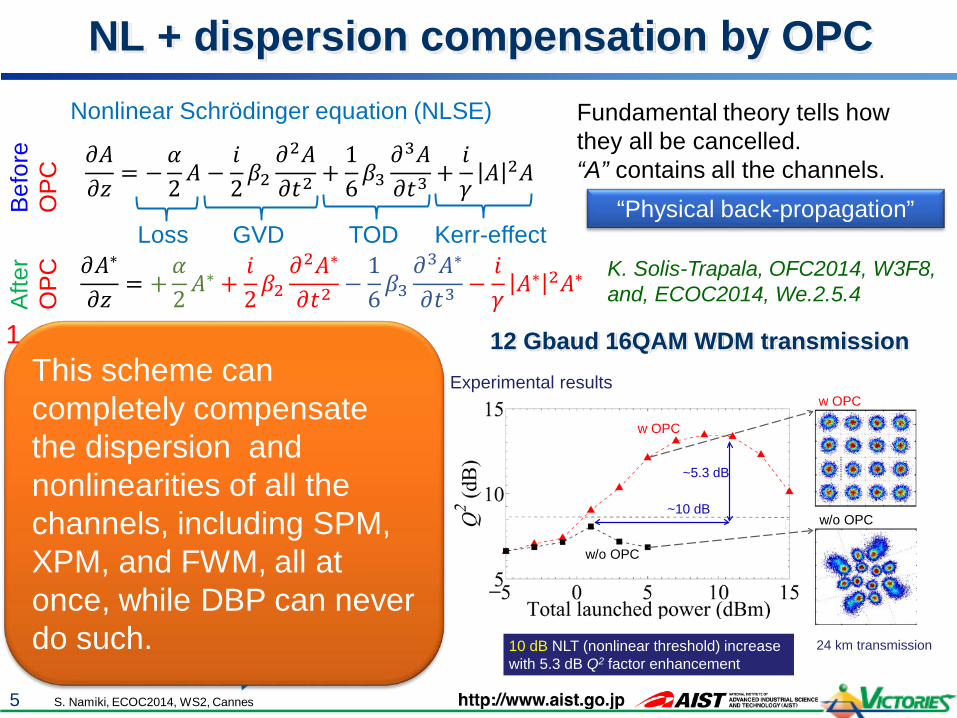
NL + dispersion compensation by OPC

5 S. Namiki, ECOC2014, WS2, Cannes

Fundamental theory tells how they all be cancelled.“A” contains all the channels.𝜕𝜕𝐴𝐴

𝜕𝜕𝑧𝑧= −

𝛼𝛼2𝐴𝐴 −

𝑖𝑖2𝛽𝛽2𝜕𝜕2𝐴𝐴𝜕𝜕𝑡𝑡2

+16𝛽𝛽3𝜕𝜕3𝐴𝐴𝜕𝜕𝑡𝑡3

+𝑖𝑖𝛾𝛾𝐴𝐴 2𝐴𝐴

Nonlinear Schrödinger equation (NLSE)

𝜕𝜕𝐴𝐴∗

𝜕𝜕𝑧𝑧= −

𝛼𝛼2𝐴𝐴∗ +

𝑖𝑖2𝛽𝛽2𝜕𝜕2𝐴𝐴∗

𝜕𝜕𝑡𝑡2 +16𝛽𝛽3𝜕𝜕3𝐴𝐴∗

𝜕𝜕𝑡𝑡3 −𝑖𝑖𝛾𝛾𝐴𝐴∗ 2𝐴𝐴∗

Loss GVD TOD Kerr-effect

Befo

reO

PCAf

ter

OPC

1. OPC based on HNLF2. Distributed Raman Amplification (DRA)

To symmetrize power excursions3. Dispersion flattened fiber (NZDSF) [1]

To satisfy GVD and TOD requirements

λpump

λTx λRx

[1] N. Kumano et al., ECOC’02 PD1.4

Actually developed fiber [1]!

12 Gbaud 16QAM WDM transmission

w/o OPC

w OPC

10 dB NLT (nonlinear threshold) increase with 5.3 dB Q2 factor enhancement

~10 dB

~5.3 dB

24 km transmission

Experimental results

w/o OPC

w OPC

K. Solis-Trapala, OFC2014, W3F8, and, ECOC2014, We.2.5.4

This scheme can completely compensate the dispersion and nonlinearities of all the channels, including SPM, XPM, and FWM, all at once, while DBP can never do such.

“Physical back-propagation”

𝜕𝜕𝐴𝐴∗

𝜕𝜕𝑧𝑧= +

𝛼𝛼2𝐴𝐴∗ +

𝑖𝑖2𝛽𝛽2𝜕𝜕2𝐴𝐴∗

𝜕𝜕𝑡𝑡2 +16𝛽𝛽3𝜕𝜕3𝐴𝐴∗

𝜕𝜕𝑡𝑡3 −𝑖𝑖𝛾𝛾 𝐴𝐴∗ 2𝐴𝐴∗

𝜕𝜕𝐴𝐴∗

𝜕𝜕𝑧𝑧= +

𝛼𝛼2𝐴𝐴∗ +

𝑖𝑖2𝛽𝛽2𝜕𝜕2𝐴𝐴∗

𝜕𝜕𝑡𝑡2 −16𝛽𝛽3𝜕𝜕3𝐴𝐴∗

𝜕𝜕𝑡𝑡3 −𝑖𝑖𝛾𝛾𝐴𝐴∗ 2𝐴𝐴∗