Parametric Schedule Estimation for Launch Vehicles

George Culver, CPP, CCEAgeorge.a.culver@saic.comSAIC Huntsville

2011 JANNAF MSS / LPS / SPS Joint Meeting, Huntsville AL

https://ntrs.nasa.gov/search.jsp?R=20120002888 2018-07-17T13:39:31+00:00Z

Rationale and Process Followed

• This investigation analyzes historical data to identify schedule drivers.

• Goal is to derive schedule estimating relationships (SERs) at the phase level.– Phase is defined as the duration between

major project milestones.

• This investigation uses a 2-pass approach.

2-Pass Approach

1. Mash Up All Data Sources

2. Filter Mission List to Those

with Complete Data

3. Organize Missions by

Phase Based on Available Data

4. Identify Driving

Technical Parameters

6. Assess Candidate Regression

Forms

7. Document Results

5. Grow Mission List by Obtaining Missing Data for

Driving Parameters

LegendFirst PassSecond Pass

Data Sources

• Technical and schedule data used in this study came primarily from three sources:1. Rutkowski schedule database2. QuickCost database3. NAFCOM 2008 database

• Additional data obtained from the REDSTAR library to fill-in missing values.

https://redstar.saic.com

Missions Assessed

AE-3 HAWKEYE SWAS S-IVB Magellan

AEM-HCMM HEAO-1 TDRS-A Skylab Airlock Mariner-6

ALEXIS HEAO-2 TOMSEP Skylab OWS Mariner-10

AMPTE-CCE HEAO-3 TOPEX Spacelab MCO

ATS-6 HST OTA UARS SRB MGS

Chandra HST SSM Apollo CSM & LM SRM Mars Odyssey

COBE LANDSAT-1 Centaur-D SSME Mars Pathfinder

CRRESS LANDSAT-4 Centaur-G’ X-33 MPL

DART LANDSAT-7 External Tank X-38 DPS NEAR

DE-1 MAGSAT Gemini Cassini Pioneer Venus

DE-2 MSTI 1 IUS CONTOUR Stardust

DSCS-II NATO III Lunar Rover Deep Impact Viking

ERBS OSO-8 OMV Galileo Voyager 2

FAST SAMPEX Shuttle Orbiter Genesis

GRO SCATHA S-II Lunar Prospector

Earth Orbiting Launch Vehicle/Manned Planetary

SER Generation Results (1 of 2)

• SERs generated with full mission set for 4 schedule durations

• In these runs, not much difference between multiplicative approaches

• Additive approach as good or worse than multiplicative• No appreciable difference with PDR as a milestone• No acceptable SERs up to CDR milestone using all missions

Phase Approach Number of Points

F‐Test   p‐value

Pearson's R‐Sq SEE

Start‐PDRMultiplicative (Mission Class Avg) 87 0.036 0.274 0.88Multiplicative (Mission Class Trim Mean) 87 0.0437 0.267 0.881Additive 87 0.0289 0.281 1.22

PDR‐CDRMultiplicative (Mission Class Avg) 82 0.0121 0.325 0.635Multiplicative (Mission Class Trim Mean) 82 0.0141 0.32 0.636Additive 82 0.0543 0.275 1.091

Start‐CDRMultiplicative (Mission Class Avg) 87 0.0279 0.282 0.58Multiplicative (Mission Class Trim Mean) 87 0.0102 0.312 0.623Additive 87 0.006 0.327 1.31

CDR‐DeliveryMultiplicative (Mission Class Avg) 61 <0.0001 0.628 0.42Multiplicative (Mission Class Trim Mean) 61 <0.0001 0.605 0.435Additive 61 0.0132 0.422 1.27

SER Generation Results (2 of 2)

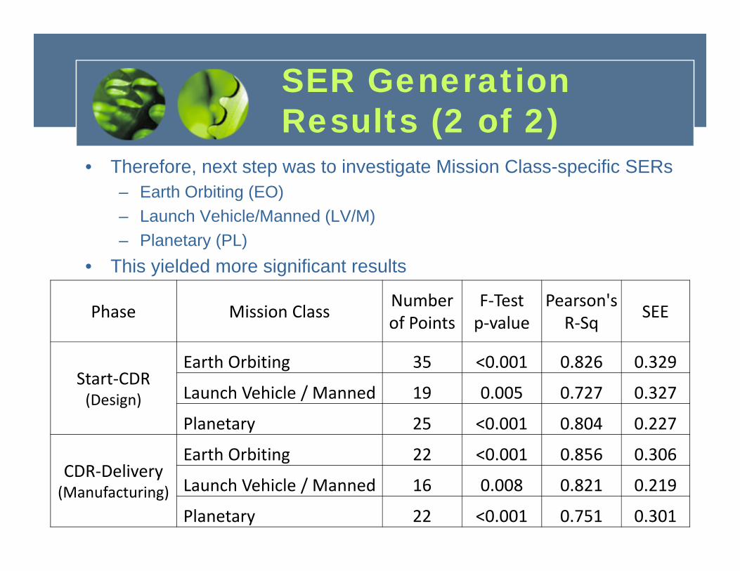
• Therefore, next step was to investigate Mission Class-specific SERs– Earth Orbiting (EO)– Launch Vehicle/Manned (LV/M)– Planetary (PL)

• This yielded more significant results

Phase Mission Class Number of Points

F‐Testp‐value

Pearson's R‐Sq SEE

Start‐CDR(Design)

Earth Orbiting 35 <0.001 0.826 0.329

Launch Vehicle / Manned 19 0.005 0.727 0.327

Planetary 25 <0.001 0.804 0.227

CDR‐Delivery(Manufacturing)

Earth Orbiting 22 <0.001 0.856 0.306

Launch Vehicle / Manned 16 0.008 0.821 0.219

Planetary 22 <0.001 0.751 0.301

Launch Vehicle/Manned SER Regression

F Test p-value = 0.005Pearson R2 = 0.727Est Std Error = 0.327

F Test p-value = 0.008Pearson R2 = 0.821Est Std Error = 0.219

508.0366.0

925.0393.0432.0124.0

089.0779.0

ReRe

877.377__

ParallelqtsPostApolloCrewedusableStreamEMStartYr

dsManufMethoFundAvailDurCDRStart

968.0730.0310.0163.0

084.0177.0

Re768.13__

ParallelqtsPostApolloCrewedStartYrPowerGenEngrMgmtDurDeliveryCDR

Independent Variable Details

• Mix of indicator and numeric variables

• Heritage to NAFCOM Management Factor definitions

• Complexity Variable is sum of normalized Dry Weight, Maximum Data Rate, and Number of Instruments– Aggregated these variables

to alleviate autocorrelation effects

– Normalized to avoid effects of scale

Regression Factor Trends

Are there any meaningful trends for SER regression factors?

• Project start year is the most common factor

• Engineering Mgmt significant in some capacity for all SERs

• Many class-specific factors significant

LegendSignificant to SER Not significant Excluded from Analysis

Regression Validation

• As a means of validation, the same data was used to generate SERs with a different regression method– Minimum Unbiased Percent Error (MUPE) selected

• Results obtained were nearly identical to log-transformed ordinary least squares (LOLS) regressions– Magnitude of coefficients changed very little—coefficients

differed by less than 12%– Statistical significance very similar– Adds credibility to LOLS results

• Addition verification performed to test fundamental assumptions of LOLS regression

LVM SER Residual Analysis—Acceptable

LVM Design SER LVM Manufacturing SER

Equal Variance Assumption: No significant trend evident, assumption valid.

Normality Assumption: Log residuals normally distributed.

Normality Assumption: Log residuals normally distributed.

Equal Variance Assumption: No significant trend evident, assumption valid.

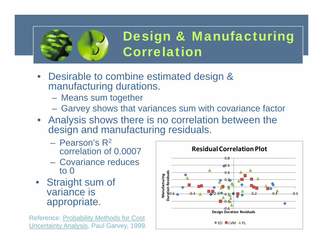
Design & Manufacturing Correlation

• Desirable to combine estimated design & manufacturing durations.– Means sum together– Garvey shows that variances sum with covariance factor

• Analysis shows there is no correlation between the design and manufacturing residuals.

‐0.6

‐0.4

‐0.2

0

0.2

0.4

0.6

0.8

‐0.6 ‐0.4 ‐0.2 0 0.2 0.4 0.6

Manufacturin

g Du

ratio

n Re

siduals

Design Duration Residuals

Residual Correlation Plot

EO LVM PL

– Pearson’s R2

correlation of 0.0007– Covariance reduces

to 0• Straight sum of

variance is appropriate.

Reference: Probability Methods for Cost Uncertainty Analysis, Paul Garvey, 1999.

SERRA Model—Inputs

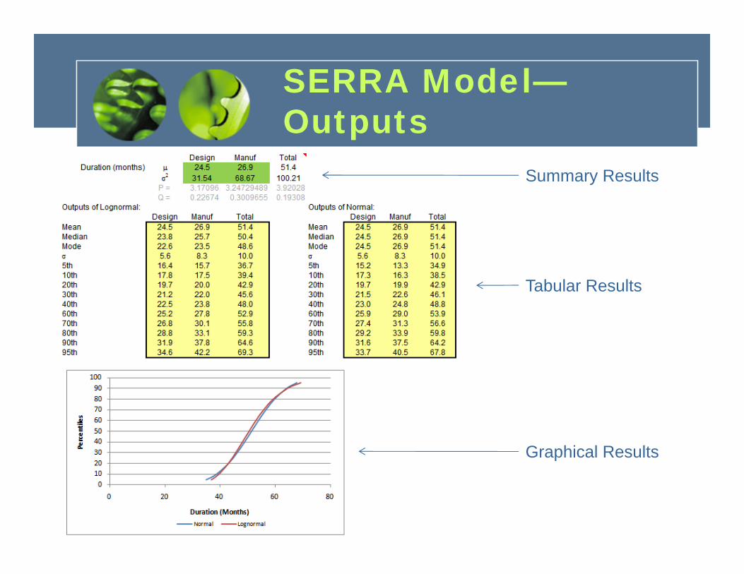
SERRA Model—Outputs

Summary Results

Tabular Results

Graphical Results

Conclusion

• Objective of this task was to investigate feasibility of SERs– Valid SERs have been generated & applied in

existing joint confidence level analyses – Statistically significant results achieved– SERs employed in a model for immediate use

• Future work– Integrate into future version of NAFCOM– Refine SERs with new missions, additional effects

SERRA Model

• Schedule Estimating Relationships Risk Assessment (SERRA) model available for distribution

• Excel-based implementation of SERs• Contact George Culver

(george.a.culver@saic.com) for a copy

SUPPORTING DATA

Earth Orbiting SER Regression

F Test p-value = <0.001Pearson R2 = 0.826Est Std Error = 0.329

F Test p-value = <0.001Pearson R2 = 0.856Est Std Error = 0.306

415.0443.0729.0260.0158.0

206.0138.0488.0203.0]1024/12/)1(5000/)50[(274.69__

MilitaryCommSatyObservatorStreamEMDesignLifeStartYrdsManufMethoTestApprMaxData

NumInstDryWtDurCDRStart

441.0437.0399.0156.0212.0

555.0504.0551.0__

BusMilitaryCommSatyObservatorDesignLifeStartYrEngrMgmtDurDeliveryCDR

Planetary SER Regression

F Test p-value = <0.001Pearson R2 = 0.804Est Std Error = 0.227

F Test p-value = <0.001Pearson R2 = 0.751Est Std Error = 0.301

599.0393.0229.0

337.0420.0759.0__RTGStreamEMDesignLife

StartYrFundAvailDurCDRStart

376.0613.0824.0065.0)]256/12/)1(4000/)100[(279.5__

RTGStartYrStreamEMMaxDataNumInstDryWtDurDeliveryCDR

EO SER Residual Analysis—Acceptable

EO Design SER EO Manufacturing SER

Equal Variance Assumption: Slight decreasing trend evident (cone), however assumption valid.

Normality Assumption: Log residuals normally distributed.

Normality Assumption: Log residuals normally distributed.

Equal Variance Assumption: No significant trend evident, assumption valid.

PL SER Residual Analysis—Acceptable

PL Design SER PL Manufacturing SER

Equal Variance Assumption: Slight decreasing trend evident (cone), however assumption valid.

Normality Assumption: Log residuals normally distributed.

Normality Assumption: Log residuals normally distributed.

Equal Variance Assumption: No significant trend evident, assumption valid.