Parameter identification of GISSMO damage model for DOCOL ...845116/FULLTEXT01.pdf · steel grade...
72
Parameter identification of GISSMO damage model for DOCOL 1200M A study on crash simulation for high strength steel sheet components Parameteridentifiering för materialmodellen GISSMO hos DOCOL 1200M En studie av brottsimulering för plåtar av höghållfast stål Daniel Hörling Faculty of science and technology Degree project for master of science in engineering, mechanical engineering 30 credit points Supervisor: Anders Gåård Examiner: Jens Bergström Date: 2015-08-10
Transcript of Parameter identification of GISSMO damage model for DOCOL ...845116/FULLTEXT01.pdf · steel grade...
Parameter identification of GISSMO damage model for DOCOL 1200M
A study on crash simulation for high strength steel sheet components
Parameteridentifiering för materialmodellen GISSMO hos DOCOL 1200M
En studie av brottsimulering för plåtar av höghållfast stål
Daniel Hörling
Faculty of science and technology
Degree project for master of science in engineering, mechanical engineering
30 credit points
Supervisor: Anders Gåård
Examiner: Jens Bergström
Date: 2015-08-10

ii
Abstract In the automotive industry there is a conflict between the need for weight reduction in order to reduce the CO2
emissions and the need for high safety. It has led to the use of high strength steel instead of the traditional
lightweight materials. The increased use of high strength steels in combination with that the shortened
development time in the automotive industry has led to the need of improved predictions of the actual crash
behavior well since a full scale crash test is both expensive and time consuming.
The damage model GISSMO is used in such crashworthiness simulations. In the present thesis the high strength
steel grade DOCOL 1200M, GISSMO damage model has a number of parameters and curves that defines when
necking and failure occurs, those have to be found. GISSMO is a phenomenological damage mechanics model
which is based on experiments and does not consider voids and cracks thus it is only reliable to similar load cases
as analyzed in the experiments. The different load cases are represented by the triaxiality which is the ratio
between the mean stress and the von Mises stress.
To find the parameters a number of test specimens were manufactured and tested in uniaxial tension then a
FEM model was designed and the force displacement curve achieved from the simulation was mapped to match
the experimentally achieved curve. The parameters were changed by the software LS-OPT® in order to increase
the match. A metamodel-based optimization was run to find the curves and parameters with feedforward
neural-networks and space filling point selection.
The result shows that GISSMO has the potential to predict the failure behavior well, when the different
specimens are optimized individually the match is good for all cases and when the simulation is examined the
necking and localization of deformation is clearly seen. When the specimens are optimized together the match is
not as good as the individual match.
In order to improve the results more precise force displacement curves from the experiments would be of
interest, for example load cells and optical measurments/strain gages could have been used to get the local
displacement and the local stress and stress state. To make the model more reliable pure shear tests and
compression tests could be used in future work. Running the optimizations for more iterations may also improve
the result.

iii
Sammanfattning I bilindustrin finns en konflikt mellan viljan att minska vikten för att ge ett lägre CO2-utsläpp och kravet på god
krocksäkerhet, detta har lett till att höghållfasta stål används istället för de traditionella lättviktsmaterialen.
Användningen av höghållfasta stål i kombination med att utvecklingstiden i bilindustrin har minskat måste
krocksimuleringarna förutsäga krockbeteendet bra då ett fullskaligt krocktest både är dyrt och tidskrävande.
Skademodellen GISSMO har undersökts för att användas med DOCOL 1200M, GISSMO skademodell har ett antal
parametrar och kurvor som definierar när instabilitet och brott uppstår, dessa måste fastställas. GISSMO är en
fenomenbaserad skademodell som är baserad på experiment och tar därför inte hänsyn till inneslutningar eller
sprickor och är därför bara pålitlig för liknande spänningsfall som de som analyserades i experimenten. De olika
spänningsfallen är representerade av triaxialiteten som är kvoten mellan medelspänningen och von Mises
spänningen.
För att hitta parametrarna tillverkades och testadess ett antal provstavar i enaxligt dragprov sen skapades en
FEM-modell och kraft-förskjutningskurvan som erhålls från simuleringen mappas för att matcha kraft-
förskjutningskurvan som erhållits från dragprovet. Parametrarna ändrades av mjukvaran LS-OPT® för att öka
matchningen. En metamodel-baserad optimering utfördes för att hitta kurvorna och parametrarna med en
feedforward neural-network och punkter jämnt fördelade över parameterrummet.
Resultatet visar att GISSMO har potential att förutsäga brottbeteendet bra, när de olika provstavarna
optimerades individuellt så är passningen god och när simuleringen undersöks ses tydligt midjebildning och
lokalisering av deformationen. När provstavarna är optimerade tillsammans är passningen inte lika god som de
individuella passningarna.
För att förbättra resultaten skulle mer exakta kraft-förskjutningskurvor vara av värde, t.ex. lastceller och optisk
mätning/trådtöjningsgivare kunde ha använts för att se den lokala förskjutningen och den lokala spänningen och
spänningstillståndet. För att göra modellen mer pålitlig kan skjuvtester och kompressionstester användas i
framtiden. Att låta optimeringen pågå i fler iterationer kan också förbättra resultatet.
iv
Contents
ABSTRACT ............................................................................................................................................................................ II
SAMMANFATTNING ............................................................................................................................................................ III
CONTENTS ......................................................................................................................................................................... IV
LIST OF FIGURES ................................................................................................................................................................. VI
LIST OF TABLES ................................................................................................................................................................ VIII
ABBREVIATIONS ................................................................................................................................................................. IX
SYMBOLS ............................................................................................................................................................................. X
1 INTRODUCTION ................................................................................................................................................................. 1
2 THEORY ............................................................................................................................................................................. 2
2.1 DAMAGE MECHANICS .............................................................................................................................................................. 2
2.1.1Forming and crash ....................................................................................................................................................... 3
2.1.2 GISSMO ....................................................................................................................................................................... 3
2.2 OPTIMIZATION ....................................................................................................................................................................... 5
2.2.1 Error measurement .................................................................................................................................................... 5
2.2.2 Metamodels and point selection ................................................................................................................................ 6
3 PURPOSE ........................................................................................................................................................................... 7
4 GOAL ................................................................................................................................................................................. 7
5 METHOD ........................................................................................................................................................................... 8
5.1 DOCOL 1200M .................................................................................................................................................................... 8
5.2 CHOICE OF SPECIMENS ............................................................................................................................................................. 8
5.2.1 Limitations .................................................................................................................................................................. 9
5.3 SIMULATION SETUP ................................................................................................................................................................. 9
5.3.1 Material ...................................................................................................................................................................... 9
5.3.2 Section ...................................................................................................................................................................... 10
5.3.3 Boundary conditions (SPC) & displacement .............................................................................................................. 11
5.3.4 Force and displacement measurement .................................................................................................................... 12
5.3.5 Solver ........................................................................................................................................................................ 12
5.4 SPECIMENS .......................................................................................................................................................................... 12
5.5 EXPERIMENTAL ..................................................................................................................................................................... 13
5.5.1 Manufacturing of specimens .................................................................................................................................... 13
5.5.2 Testing ...................................................................................................................................................................... 13
5.6 OPTIMIZATION ..................................................................................................................................................................... 14
5.7 MESH SIZE DEPENDENCY ......................................................................................................................................................... 16
6 RESULTS .......................................................................................................................................................................... 17
6.1 SINGLE CASE PARAMETER IDENTIFICATIONS ................................................................................................................................ 17
6.1.1 Shear 0° .................................................................................................................................................................... 17
6.1.2 Shear 45° .................................................................................................................................................................. 18
6.1.3 Shear 60° .................................................................................................................................................................. 20
6.1.4 Notched .................................................................................................................................................................... 21
6.1.5 Double Notched ........................................................................................................................................................ 23
6.1.6 Mini tensile ............................................................................................................................................................... 24
6.2 MULTI CASE PARAMETER IDENTIFICATIONS ................................................................................................................................. 27
6.2.1 Validation, shear 60° ................................................................................................................................................ 30
v
6.3 MESH SIZE DEPENDENCY ......................................................................................................................................................... 30
7 DISCUSSION .................................................................................................................................................................... 32
7.1 ERROR SOURCES ................................................................................................................................................................... 33
7.2 FUTURE WORK...................................................................................................................................................................... 33
8 CONCLUSION .................................................................................................................................................................. 33
9 ACKNOWLEDGEMENTS ................................................................................................................................................... 34
10 REFERENCES .................................................................................................................................................................. 35
APPENDIX A: DRAWINGS OF THE SPECIMENS .................................................................................................................... 37
A.1 SHEAR 0° ............................................................................................................................................................................ 37
A.2 SHEAR 45° .......................................................................................................................................................................... 38
A.3 SHEAR 60° .......................................................................................................................................................................... 39
A.4 NOTCHED ............................................................................................................................................................................ 40
A.5 DOUBLE NOTCH .................................................................................................................................................................... 41
A.6 MINI TENSILE ....................................................................................................................................................................... 42
APPENDIX B: UNIAXIAL TENSION TEST CURVES ................................................................................................................. 43
B.1 SHEAR 0° ............................................................................................................................................................................ 43
B.2 SHEAR 45° .......................................................................................................................................................................... 43
B.3 SHEAR 60° .......................................................................................................................................................................... 44
B.4 NOTCHED ............................................................................................................................................................................ 45
B.5 DOUBLE NOTCH .................................................................................................................................................................... 45
B.6 MINI TENSILE ....................................................................................................................................................................... 46
APPENDIX C: CONVERGENCE PLOTS ................................................................................................................................... 47
C.1 SHEAR 0° ............................................................................................................................................................................ 47
C.2 SHEAR 45° .......................................................................................................................................................................... 49
C.3 SHEAR 60° .......................................................................................................................................................................... 51
C.4 NOTCHED ............................................................................................................................................................................ 53
C.5 DOUBLE NOTCHED ................................................................................................................................................................ 55
C.6 MINI TENSILE ....................................................................................................................................................................... 57
C.7 MULTI CASE ......................................................................................................................................................................... 59
vi
List of figures FIGURE 1. A SCHEMATIC VIEW TO SHOW THE MANY SAFETY COMPONENTS USED IN A MODERN CAR [4]. ............................................................ 1
FIGURE 2. THE DIFFERENT SAFETY ZONES OF A CAR [6]. ............................................................................................................................ 1
FIGURE 3. INFLUENCE OF THE FADING EXPONENT M [11]. ......................................................................................................................... 5
FIGURE 4. ADAPTION OF A SUBREGION: (A) PURE PANNING, (B) PURE ZOOMING, (C) COMBINATION OF BOTH [14]. ............................................. 6
FIGURE 5. SCHEMATIC OF A NEURAL NETWORK WITH 2 INPUTS AND A HIDDEN LAYER OF 4 NEURONS [17]. ......................................................... 6
FIGURE 6. A SPACE FILLING DESIGN WITH 5 POINTS IN A 2D BOX [14]. ........................................................................................................ 7
FIGURE 7. A CROSS SECTION SEEN IN A LIGHT MICROSCOPE ETCHED IN 3% NITAL [20]. .................................................................................. 8
FIGURE 8. TYPICAL FAILURE CURVE FOR SHEET METAL MODELED WITH SHELL ELEMENTS [13]. .......................................................................... 9
FIGURE 9. LS-PREPOST MATERIAL KEYWORD FOR THE MATERIAL USED IN THE SIMULATIONS, THE UNITS USED ARE ACCORDING TO B) AT P. 2-25 IN
[22]. ..................................................................................................................................................................................... 9
FIGURE 10. TRUE STRESS-TRUE STRAIN CURVE FOR DOCOL 1200M OBTAINED AT THE SSAB STRUCTURAL R&D WORKSHOP. ........................... 10
FIGURE 11. THE LS-PREPOST MATERIAL CARD *MAT_ADD_EROSION FOR THE GISSMO PARAMETERS. .................................................. 10
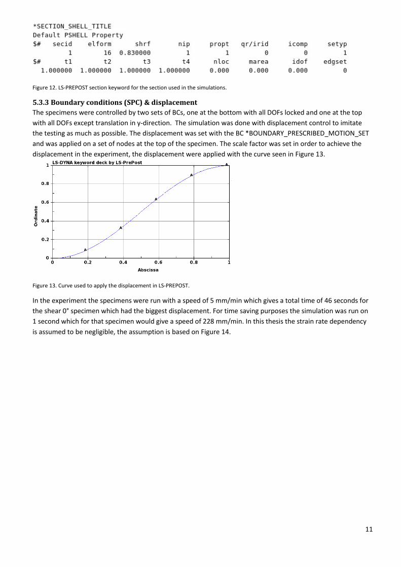
FIGURE 12. LS-PREPOST SECTION KEYWORD FOR THE SECTION USED IN THE SIMULATIONS. ......................................................................... 11
FIGURE 13. CURVE USED TO APPLY THE DISPLACEMENT IN LS-PREPOST. .................................................................................................. 11
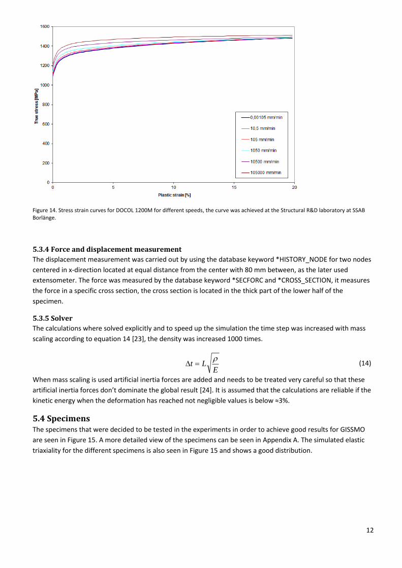
FIGURE 14. STRESS STRAIN CURVES FOR DOCOL 1200M FOR DIFFERENT SPEEDS, THE CURVE WAS ACHIEVED AT THE STRUCTURAL R&D LABORATORY
AT SSAB BORLÄNGE. .............................................................................................................................................................. 12
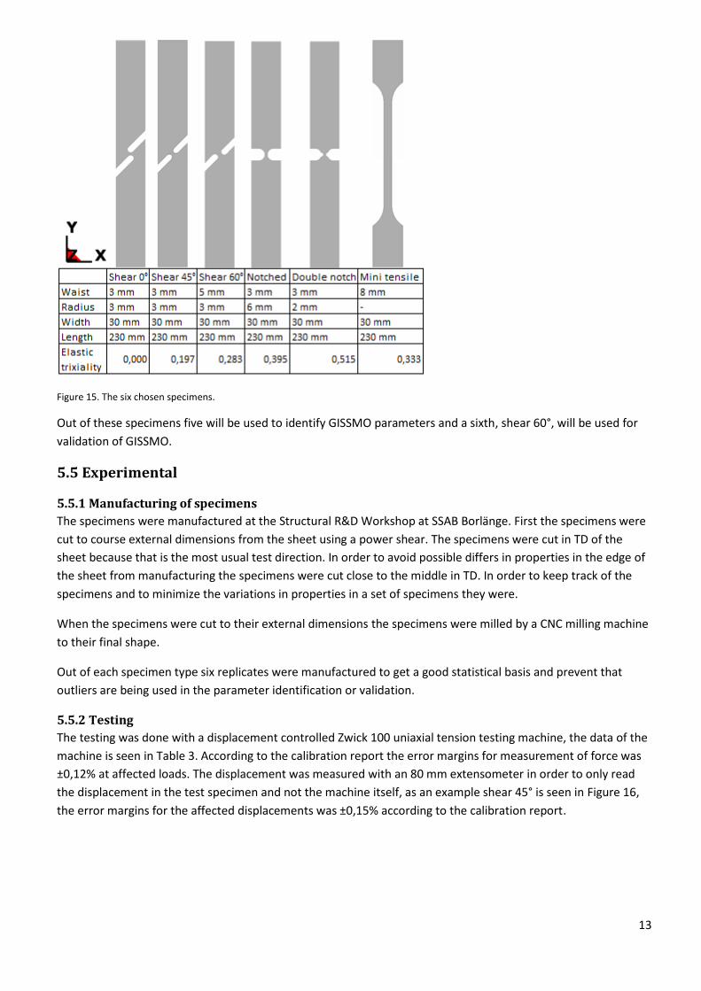
FIGURE 15. THE SIX CHOSEN SPECIMENS. ............................................................................................................................................. 13
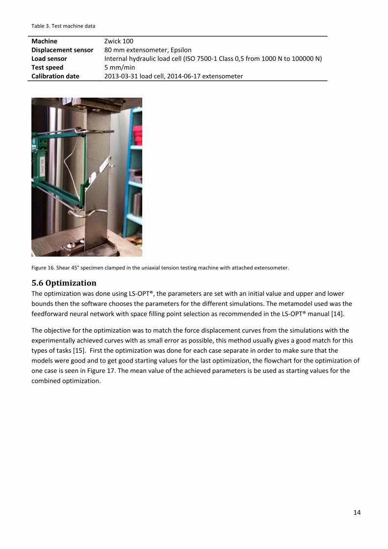
FIGURE 16. SHEAR 45° SPECIMEN CLAMPED IN THE UNIAXIAL TENSION TESTING MACHINE WITH ATTACHED EXTENSOMETER. ............................... 14
FIGURE 17. SCREENSHOT OF THE FLOWCHART IN LS-OPT® DESCRIBING THE OPTIMIZATION OF THE DOUBLE NOTCH SPECIMEN TYPE. .................... 15
FIGURE 18. SCREENSHOT OF THE FLOWCHART IN LS-OPT® DESCRIBING THE OPTIMIZATION. ......................................................................... 15
FIGURE 19. THE GISSMO INSTABILITY AND FAILURE CRITERIA CURVES FOR THE SHEAR 0° SPECIMEN. .............................................................. 17
FIGURE 20. FORCE DISPLACEMENT CURVES FOR THE SHEAR 0° SPECIMEN BOTH EXPERIMENTAL DATA AND THE GISSMO SIMULATION. .................. 17
FIGURE 21. THE SHEAR 0° SPECIMEN AT DIFFERENT STATES OF DEFORMATION A) START OF PLASTIC DEFORMATION B) LOCALIZATION OF PLASTIC
DEFORMATION C) HEAVILY PLASTICALLY DEFORMED D) FAILURE E) A PHOTO OF THE EXPERIMENTALLY FAILED SPECIMEN. ............................. 18
FIGURE 22. THE AMOUNT OF KINETIC ENERGY VS. WITH DISPLACEMENT IN THE CALCULATION FOR THE SHEAR 0° SPECIMEN. ................................ 18
FIGURE 23. THE GISSMO INSTABILITY AND FAILURE CRITERIA CURVES FOR THE SHEAR 45° SPECIMEN. ............................................................ 19
FIGURE 24. FORCE DISPLACEMENT CURVES FOR THE SHEAR 45° SPECIMEN BOTH EXPERIMENTAL DATA AND THE GISSMO SIMULATION. ................ 19
FIGURE 25. THE SHEAR 45° SPECIMEN AT DIFFERENT STATES OF DEFORMATION A) START OF PLASTIC DEFORMATION B) LOCALIZATION OF PLASTIC
DEFORMATION C) HEAVILY PLASTICALLY DEFORMED D) FAILURE E) A PHOTO OF THE EXPERIMENTALLY FAILED SPECIMEN. ............................. 19
FIGURE 26. THE AMOUNT OF KINETIC ENERGY VS. WITH DISPLACEMENT IN THE CALCULATION FOR THE SHEAR 45° SPECIMEN. .............................. 20
FIGURE 27. THE GISSMO INSTABILITY AND FAILURE CRITERIA CURVES FOR THE SHEAR 60° SPECIMEN. ............................................................ 20
FIGURE 28. FORCE DISPLACEMENT CURVES FOR THE SHEAR 60° SPECIMEN BOTH EXPERIMENTAL DATA AND THE GISSMO SIMULATION. ................ 21
FIGURE 29. THE SHEAR 60° SPECIMEN AT DIFFERENT STATES OF DEFORMATION A) START OF PLASTIC DEFORMATION B) LOCALIZATION OF PLASTIC
DEFORMATION C) HEAVILY PLASTICALLY DEFORMED D) FAILURE E) A PHOTO OF THE EXPERIMENTALLY FAILED SPECIMEN. ............................. 21
FIGURE 30. THE AMOUNT OF KINETIC ENERGY VS. WITH DISPLACEMENT IN THE CALCULATION FOR THE SHEAR 60° SPECIMEN. .............................. 21
FIGURE 31. THE GISSMO INSTABILITY AND FAILURE CRITERIA CURVES FOR THE NOTCHED SPECIMEN............................................................... 22
FIGURE 32. FORCE DISPLACEMENT CURVES FOR THE NOTCHED SPECIMEN BOTH EXPERIMENTAL DATA AND THE GISSMO SIMULATION. ................. 22
FIGURE 33. THE NOTCHED SPECIMEN AT DIFFERENT STATES OF DEFORMATION A) START OF PLASTIC DEFORMATION B) LOCALIZATION OF PLASTIC
DEFORMATION C) HEAVILY PLASTICALLY DEFORMED D) FAILURE E) A PHOTO OF THE EXPERIMENTALLY FAILED SPECIMEN. ............................. 23
FIGURE 34. THE AMOUNT OF KINETIC ENERGY VS. WITH DISPLACEMENT IN THE CALCULATION FOR THE NOTCHED SPECIMEN. ................................ 23
FIGURE 35. THE GISSMO INSTABILITY AND FAILURE CRITERIA CURVES FOR THE DOUBLE NOTCHED SPECIMEN. .................................................. 23
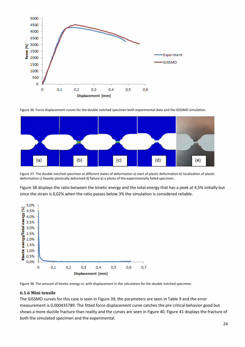
FIGURE 36. FORCE DISPLACEMENT CURVES FOR THE DOUBLE NOTCHED SPECIMEN BOTH EXPERIMENTAL DATA AND THE GISSMO SIMULATION. ...... 24
FIGURE 37. THE DOUBLE NOTCHED SPECIMEN AT DIFFERENT STATES OF DEFORMATION A) START OF PLASTIC DEFORMATION B) LOCALIZATION OF
PLASTIC DEFORMATION C) HEAVILY PLASTICALLY DEFORMED D) FAILURE E) A PHOTO OF THE EXPERIMENTALLY FAILED SPECIMEN. .................. 24
FIGURE 38. THE AMOUNT OF KINETIC ENERGY VS. WITH DISPLACEMENT IN THE CALCULATION FOR THE DOUBLE NOTCHED SPECIMEN. .................... 24
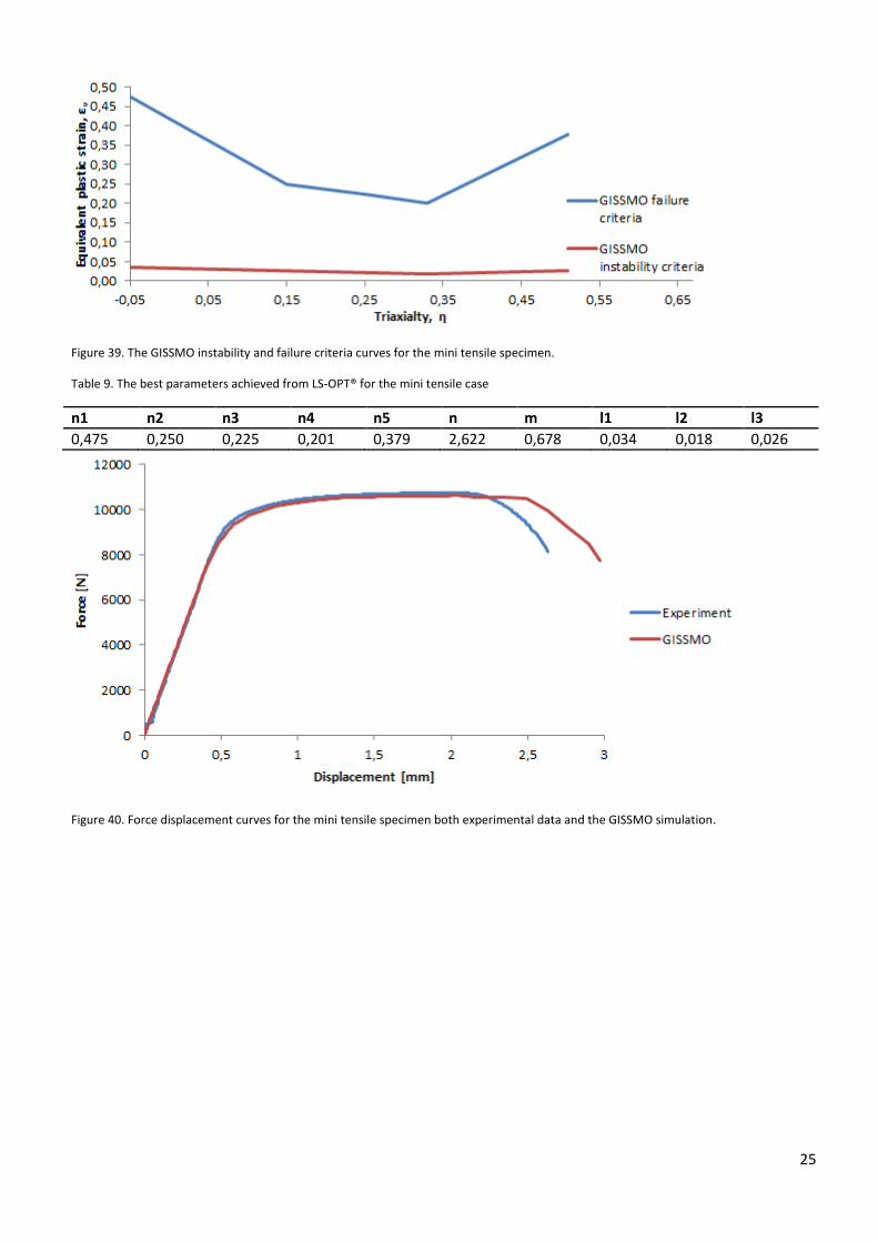
FIGURE 39. THE GISSMO INSTABILITY AND FAILURE CRITERIA CURVES FOR THE MINI TENSILE SPECIMEN. ......................................................... 25
FIGURE 40. FORCE DISPLACEMENT CURVES FOR THE MINI TENSILE SPECIMEN BOTH EXPERIMENTAL DATA AND THE GISSMO SIMULATION. ............. 25
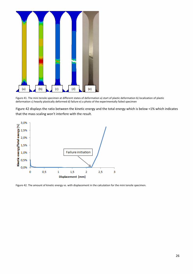
FIGURE 41. THE MINI TENSILE SPECIMEN AT DIFFERENT STATES OF DEFORMATION A) START OF PLASTIC DEFORMATION B) LOCALIZATION OF PLASTIC
DEFORMATION C) HEAVILY PLASTICALLY DEFORMED D) FAILURE E) A PHOTO OF THE EXPERIMENTALLY FAILED SPECIMEN .............................. 26
FIGURE 42. THE AMOUNT OF KINETIC ENERGY VS. WITH DISPLACEMENT IN THE CALCULATION FOR THE MINI TENSILE SPECIMEN. ........................... 26
FIGURE 43. THE GISSMO INSTABILITY AND FAILURE CRITERIA CURVES FOR DOCOL 1200M. ....................................................................... 27
vii
FIGURE 44. FORCE DISPLACEMENT CURVES FOR THE SHEAR 0° SPECIMEN BOTH EXPERIMENTAL DATA AND THE GISSMO SIMULATION WITH THE FINAL
GISSMO PARAMETER FOR DOCOL 1200M. ............................................................................................................................. 28
FIGURE 45. FORCE DISPLACEMENT CURVES FOR THE SHEAR 45° SPECIMEN BOTH EXPERIMENTAL DATA AND THE GISSMO SIMULATION WITH THE
FINAL GISSMO PARAMETER FOR DOCOL 1200M. ..................................................................................................................... 28
FIGURE 46. FORCE DISPLACEMENT CURVES FOR THE NOTCHED SPECIMEN BOTH EXPERIMENTAL DATA AND THE GISSMO SIMULATION WITH THE FINAL
GISSMO PARAMETER FOR DOCOL 1200M. ............................................................................................................................. 29
FIGURE 47. FORCE DISPLACEMENT CURVES FOR THE DOUBLE NOTCHED SPECIMEN BOTH EXPERIMENTAL DATA AND THE GISSMO SIMULATION WITH
THE FINAL GISSMO PARAMETER FOR DOCOL 1200M. ............................................................................................................... 29
FIGURE 48. FORCE DISPLACEMENT CURVES FOR THE MINI TENSILE SPECIMEN BOTH EXPERIMENTAL DATA AND THE GISSMO SIMULATION WITH THE
FINAL GISSMO PARAMETER FOR DOCOL 1200M. ..................................................................................................................... 30
FIGURE 49. FORCE DISPLACEMENT CURVES FOR THE MINI TENSILE SPECIMEN BOTH EXPERIMENTAL DATA AND THE GISSMO SIMULATION WITH THE
FINAL GISSMO PARAMETER FOR DOCOL 1200M. ..................................................................................................................... 30
FIGURE 50. FORCE DISPLACEMENT CURVES FOR THE MINI TENSILE SPECIMEN WITH DIFFERENT ELEMENT SIZES. .................................................. 31
FIGURE 51. A BAD MATCH THAT WILL GENERATE A SMALL ERROR. ............................................................................................................ 32
FIGURE 52. FORCE DISPLACEMENT CURVE FROM THE UNIAXIAL TENSION TEST FOR THE SHEAR 0° SPECIMEN TYPE. .............................................. 43
FIGURE 53. FORCE DISPLACEMENT CURVE FROM THE UNIAXIAL TENSION TEST FOR THE SHEAR 45° SPECIMEN TYPE. ............................................ 44
FIGURE 54. FORCE DISPLACEMENT CURVE FROM THE UNIAXIAL TENSION TEST FOR THE SHEAR 60° SPECIMEN TYPE. ............................................ 44
FIGURE 55. FORCE DISPLACEMENT CURVE FROM THE UNIAXIAL TENSION TEST FOR THE NOTCHED SPECIMEN TYPE............................................... 45
FIGURE 56. FORCE DISPLACEMENT CURVE FROM THE UNIAXIAL TENSION TEST FOR THE DOUBLE NOTCHED SPECIMEN TYPE. .................................. 46
FIGURE 57. FORCE DISPLACEMENT CURVE FROM THE UNIAXIAL TENSION TEST FOR THE MINI TENSILE SPECIMEN TYPE. ......................................... 46

viii
List of tables TABLE 1. MECHANICAL PROPERTIES FOR DOCOL 1200M IN TRANSVERSE DIRECTION [18] [19] ..................................................................... 8
TABLE 2. CHEMICAL COMPOSITION FOR DOCOL 1200M [19] ................................................................................................................. 8
TABLE 3. TEST MACHINE DATA ........................................................................................................................................................... 14
TABLE 4. THE BEST PARAMETERS ACHIEVED FROM LS-OPT® FOR THE SHEAR 0° CASE ................................................................................... 17
TABLE 5. THE BEST PARAMETERS ACHIEVED FROM LS-OPT® FOR THE SHEAR 45° CASE ................................................................................. 19
TABLE 6. THE BEST PARAMETERS ACHIEVED FROM LS-OPT® FOR THE SHEAR 60° CASE ................................................................................. 20
TABLE 7. THE BEST PARAMETERS ACHIEVED FROM LS-OPT® FOR THE NOTCHED CASE .................................................................................. 22
TABLE 8. THE BEST PARAMETERS ACHIEVED FROM LS-OPT® FOR THE DOUBLE NOTCHED CASE ....................................................................... 23
TABLE 9. THE BEST PARAMETERS ACHIEVED FROM LS-OPT® FOR THE MINI TENSILE CASE .............................................................................. 25
TABLE 10. THE BEST PARAMETERS ACHIEVED FROM LS-OPT® FOR DOCOL 1200M ................................................................................... 27
TABLE 11. THE ERROR MEASURES FOR SHEAR 0°, SHEAR 45°, NOTCHED, DOUBLE NOTCHED AND MINI TENSILE FOR GISSMO DAMAGE MODEL FOR
DOCOL 1200M ................................................................................................................................................................... 27

ix
Abbreviations
VHSS Very High Strength Steel
GISSMO Generalized Incremental Stress-State dependent damage Model
FEM Finite Element Method
RD Rolling Direction
TD Transverse Direction
2D Two Dimensional
BC Boundary Condition
DOF Degree Of Freedom
x
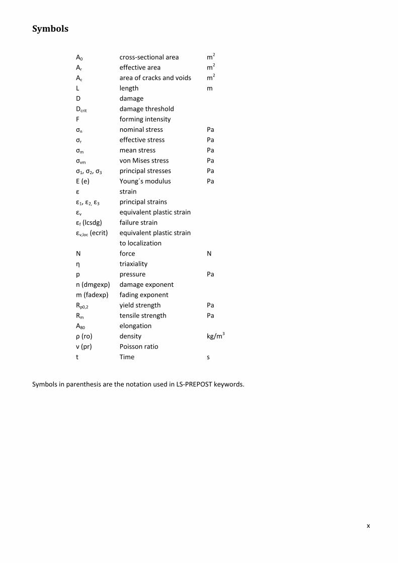
Symbols
A0 cross-sectional area m2
Ar effective area m2
Ac area of cracks and voids m2
L length m
D damage
Dcrit damage threshold
F forming intensity
σn nominal stress Pa
σr effective stress Pa
σm mean stress Pa
σvm von Mises stress Pa
σ1, σ2, σ3 principal stresses Pa
E (e) Young´s modulus Pa
ε strain
ε1, ε2, ε3 principal strains
εv equivalent plastic strain
εf (lcsdg) failure strain
εv,loc (ecrit) equivalent plastic strain
to localization
N force N
η triaxiality
p pressure Pa
n (dmgexp) damage exponent
m (fadexp) fading exponent
Rp0,2 yield strength Pa
Rm tensile strength Pa
A80 elongation
ρ (ro) density kg/m3
ν (pr) Poisson ratio
t Time s
Symbols in parenthesis are the notation used in LS-PREPOST keywords.
1
1 Introduction One of the main ideas of car chassis is to decrease the consequences from accidents in traffic, which is done by
different safety components. 73% of the CO2 emitted by a gasoline driven car occurs during usage and is
significantly influenced by car weight [1]. More safety components will give heavier cars which is in conflict with
the demand for cars with lower CO2 emissions since it will consume more fuel.
High safety and crashworthiness still applies and is in conflict with CO2 emissions regarding weight reductions
but it is hard to completely remove a safety component. A modern car contains many safety components to
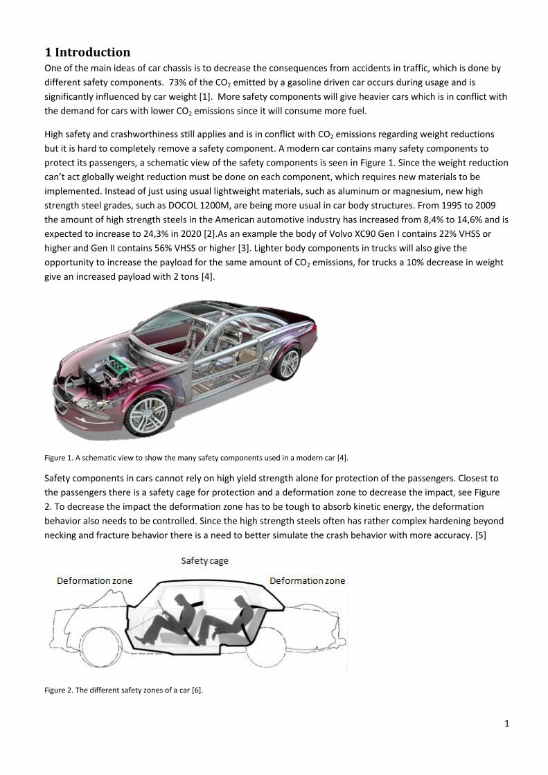
protect its passengers, a schematic view of the safety components is seen in Figure 1. Since the weight reduction
can’t act globally weight reduction must be done on each component, which requires new materials to be
implemented. Instead of just using usual lightweight materials, such as aluminum or magnesium, new high
strength steel grades, such as DOCOL 1200M, are being more usual in car body structures. From 1995 to 2009
the amount of high strength steels in the American automotive industry has increased from 8,4% to 14,6% and is
expected to increase to 24,3% in 2020 [2].As an example the body of Volvo XC90 Gen I contains 22% VHSS or
higher and Gen II contains 56% VHSS or higher [3]. Lighter body components in trucks will also give the
opportunity to increase the payload for the same amount of CO2 emissions, for trucks a 10% decrease in weight
give an increased payload with 2 tons [4].
Figure 1. A schematic view to show the many safety components used in a modern car [4].
Safety components in cars cannot rely on high yield strength alone for protection of the passengers. Closest to
the passengers there is a safety cage for protection and a deformation zone to decrease the impact, see Figure
2. To decrease the impact the deformation zone has to be tough to absorb kinetic energy, the deformation
behavior also needs to be controlled. Since the high strength steels often has rather complex hardening beyond
necking and fracture behavior there is a need to better simulate the crash behavior with more accuracy. [5]
Figure 2. The different safety zones of a car [6].
2
Crashworthiness simulations are used to develop safety components in the automotive industry. The simulations
may also give valuable information and understanding about different phenomena in a car crash. Besides that
crashing a car is expensive it is not reproducible due to variations in manufacturing. Since the development time
to launch a new car has been shortened and the demand for better crashworthiness and passive safety the
manufacturers have to rely more on crashworthiness simulations than before. [7]
This thesis was performed at SSAB Knowledge Service Center in Borlänge and is aimed to increase the
predictiveness of crashworthiness simulations. The damage model GISSMO will be investigated and the
parameters needed to fit the model to DOCOL 1200M will be identified. The identification will be done by
different specimens tested in uniaxial tension then simulated with LS-DYNA® and optimized with LS-OPT®.
2 Theory
2.1 Damage mechanics A material subjected to mechanical loading will develop damage with increased loading, the damage may occur
as voids or micro cracks. A field of research that has been active the last couple of years to incorporate damage
in constitutive model for materials, this is called damage mechanics. Damage mechanics may be divided into two
types of models, micromechanical damage mechanics models and phenomenological damage mechanics
models, the later model will be used in this thesis but below both models are shortly described.
Micromechanical damage mechanics models are based on damage mechanisms on micro level such as voids and
micro cracks and have defined micromechanical criteria for damage growth, this is then derived to macroscopic
models. Since this is based on actual physical mechanisms it is reliable applying to new loading scenarios and
new material but it is difficult to develop a realistic model and there are uncertainties regarding the
micromechanical criteria for damage growth.
Phenomenological damage mechanics models is based on actual experiments where the material is subjected to
different load cases where the damage, stresses and strains or forces and displacements are recorded. The
damage is hard to measure so often it is an estimation done from for example changes in stiffness. These types
of models should be used with extra attention when tested for other load cases then what was used when the
model was developed since it’s not based on any physical damage mechanisms. [8]
One way to describe the damage is to look at the cross-sectional area of the material, A0, and compare it with
the effective area, Ar. Due to voids and micro cracks of a certain area, Ac, the effective area will be as equation 1.
cr AAA 0 (1)
Due to the effect of closed voids and micro cracks the effective area might be even smaller than proposed in
equation 1. The damage, D, will then be stated as equation 2 where D=0 corresponds to the undamaged
material and D=1 corresponds to failure and separation of the material into two parts and values in between
displays the amount of damage. [9]
0
0
A
AAD r (2)
The effective stress, σr, may then be expressed as a function of nominal stress, σn, see equation 3, or as a
function of strain, equation 4. [8]
3
n
rr
rDA
A
A
N
A
N
1
10
0
(3)
EDr 1 (4)
2.1.1Forming and crash
In forming the post-critical behavior is of no interest due the fact that instability and necking is considered as
failure. In automotive industry and crashworthiness simulations the post-critical behavior is of highly importance
because a maximum use of energy is of interest and that can only be achieved by use of the total ductility of a
material. One way to do this is by use of these models mentioned above, the reason that the forming history
must be considered when doing a crashworthiness simulation is that often the properties of the material
assumed to be in delivery conditions but they are always plastically deformed to its final form. Crashworthiness
simulations usually use constitutive models such as von Mises flow rule or the Gurson, Tveergard & Needleman
approach while forming simulations uses an anisotropic yield description often based on the Hill or Barlat
criteria [10]. This demands for a history dependent damage model that are able to consider the change of
properties from forming and changes in strain path when the material is deformed until crash. [11]
2.1.2 GISSMO
At Daimler AG and DYNAmore a material model called GISSMO has been developed. The main issue with
GISSMO is to combine the damage models for crashworthiness simulations and the models for localization and
instability used for forming applications. Doing that will increase the accuracy in crashworthiness simulation and
the more accurate the simulations are less practical tests needs to be carried out. GISSMO is a
phenomenological damage mechanics model, as described earlier, and uses a constitutive model to predict the
uniformly plastic behavior before necking.
To be able to catch the unstable plastic behavior after necking a curve describing the onset of necking from
experiments is iteratively used as a weighting function for the simulation since the stress state varies with plastic
deformation. [10]
In crashworthiness simulations the stress is usually represented by the stress triaxiality, equation 5.
vm
m
(5)
Since plain stress is a common assumption for sheet metals the mean stress, σm, is given with σ3=0, equation 6.
[10]
pm
3
21 (6)
Equation 7 displays the von Mises stress for the plane stress assumption (σ3=0) [12].
21
2
2
2
1 vm (7)
4
Since GISSMO calculates in increment it is path dependent and will give different final results for different strain
paths. In order to allow different strain paths when predicting failure the idea of a measurement of damage has
been further developed, see equation 8.
v
n
f
Dn
D
11
(8)
21
2
2
2
13
2 v (9)
Where the exponent n allows for nonlinear representation of the damage, which makes it possible to simulate
both forming and crash more accurate. Δεv is the notation for the incremental step in equivalent plastic strain,
see equation 9, and εf is the triaxiality dependent failure strain. This failure strain is received by experiments and
inserted into the system as a failure strain vs. triaxiality curve which makes the simulation flexible to different
triaxialities, an example of this curve can be seen in Figure 8.
In order to simulate the instability of the material the formability intensity is introduced it may be looked at as a
measure of remaining formability before instability occurs, the linear forming intensity, F, is seen in equation 10.
locv
vF,
(10)
Where εv,loc is defined as the equivalent plastic strain to localization and is dependent of the triaxiality that is
introduced to the system as a curve. F=0 corresponds to the undeformed material and F=1 corresponds to the
point where necking occurs. Equation 10 has been developed to equation 11 in order to cover nonlinear plastic
deformation as what was done with the damage parameter.
v
n
locv
Fn
F
11
,
(11)
The forming intensity is achieved in the same way as the damage parameter, the difference is the use of a curve
of limit strain vs. triaxiality for the forming intensity and a curve of failure strain vs. triaxiality for the damage
parameter.
A damage threshold, Dcrit, is defined either as a fixed value or as a function of the forming intensity at the actual
state of deformation. When the damage reaches this curve for the actual triaxiality the damage threshold will be
stored for the actual element and the flow stress and the damage will be coupled and the effective stress tensor
is defined according to equation 12 with the fading exponent m. [13]
m
crit
critnr
D
DD
11 (12)
5
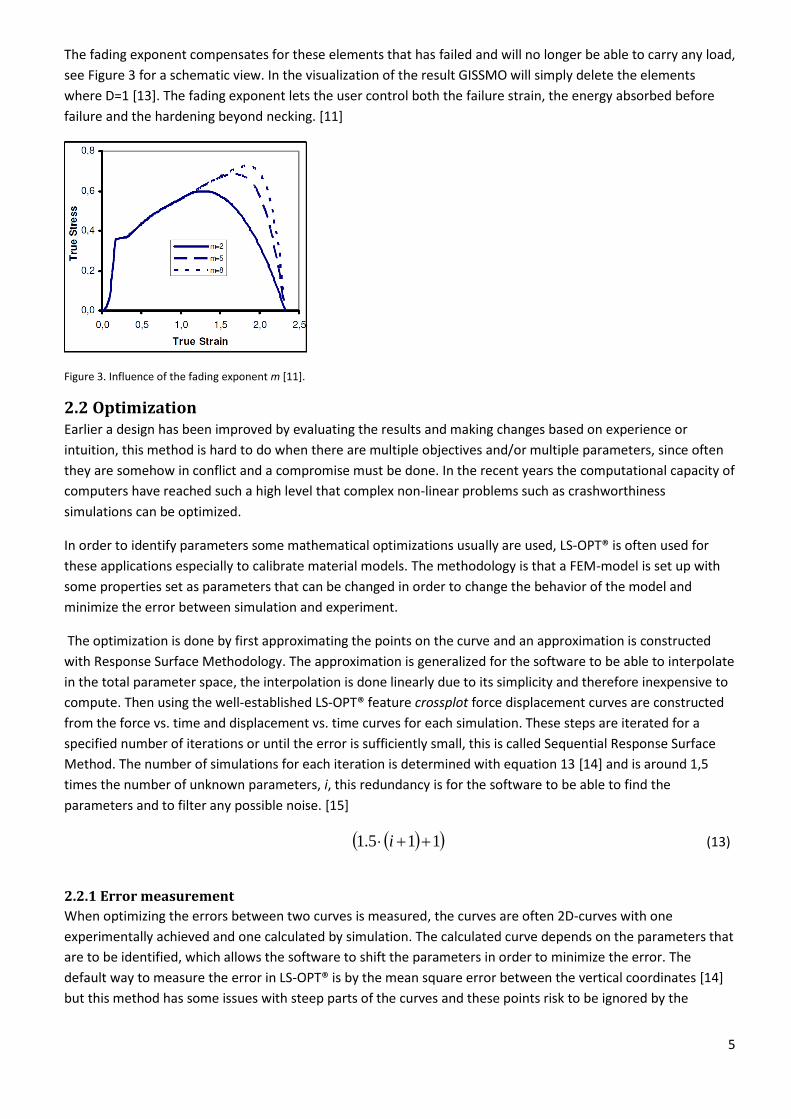
The fading exponent compensates for these elements that has failed and will no longer be able to carry any load,
see Figure 3 for a schematic view. In the visualization of the result GISSMO will simply delete the elements
where D=1 [13]. The fading exponent lets the user control both the failure strain, the energy absorbed before
failure and the hardening beyond necking. [11]
Figure 3. Influence of the fading exponent m [11].
2.2 Optimization Earlier a design has been improved by evaluating the results and making changes based on experience or
intuition, this method is hard to do when there are multiple objectives and/or multiple parameters, since often
they are somehow in conflict and a compromise must be done. In the recent years the computational capacity of
computers have reached such a high level that complex non-linear problems such as crashworthiness
simulations can be optimized.
In order to identify parameters some mathematical optimizations usually are used, LS-OPT® is often used for
these applications especially to calibrate material models. The methodology is that a FEM-model is set up with
some properties set as parameters that can be changed in order to change the behavior of the model and
minimize the error between simulation and experiment.
The optimization is done by first approximating the points on the curve and an approximation is constructed
with Response Surface Methodology. The approximation is generalized for the software to be able to interpolate
in the total parameter space, the interpolation is done linearly due to its simplicity and therefore inexpensive to
compute. Then using the well-established LS-OPT® feature crossplot force displacement curves are constructed
from the force vs. time and displacement vs. time curves for each simulation. These steps are iterated for a
specified number of iterations or until the error is sufficiently small, this is called Sequential Response Surface
Method. The number of simulations for each iteration is determined with equation 13 [14] and is around 1,5
times the number of unknown parameters, i, this redundancy is for the software to be able to find the
parameters and to filter any possible noise. [15]
115.1 i (13)
2.2.1 Error measurement
When optimizing the errors between two curves is measured, the curves are often 2D-curves with one
experimentally achieved and one calculated by simulation. The calculated curve depends on the parameters that
are to be identified, which allows the software to shift the parameters in order to minimize the error. The
default way to measure the error in LS-OPT® is by the mean square error between the vertical coordinates [14]
but this method has some issues with steep parts of the curves and these points risk to be ignored by the
6
software, as is known force displacement curves from tension tests tend to have a steep decline just before
failure. [15]
To catch the behavior for all parts of the curve partial curve mapping is used, this method uses the area between
the two 2D-curves and shifts the parameters to minimize the area. The algorithm used by LS-OPT® to compute
the area between the curves can be seen in more detail in [14] and [15].
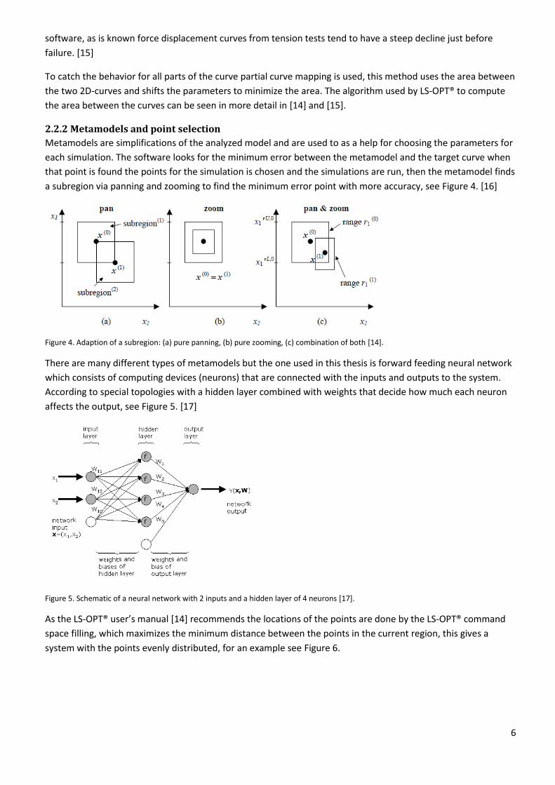
2.2.2 Metamodels and point selection
Metamodels are simplifications of the analyzed model and are used to as a help for choosing the parameters for
each simulation. The software looks for the minimum error between the metamodel and the target curve when
that point is found the points for the simulation is chosen and the simulations are run, then the metamodel finds
a subregion via panning and zooming to find the minimum error point with more accuracy, see Figure 4. [16]
Figure 4. Adaption of a subregion: (a) pure panning, (b) pure zooming, (c) combination of both [14].
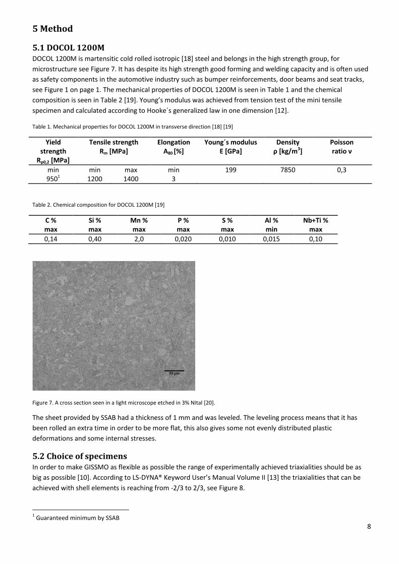
There are many different types of metamodels but the one used in this thesis is forward feeding neural network
which consists of computing devices (neurons) that are connected with the inputs and outputs to the system.
According to special topologies with a hidden layer combined with weights that decide how much each neuron
affects the output, see Figure 5. [17]
Figure 5. Schematic of a neural network with 2 inputs and a hidden layer of 4 neurons [17].
As the LS-OPT® user’s manual [14] recommends the locations of the points are done by the LS-OPT® command
space filling, which maximizes the minimum distance between the points in the current region, this gives a
system with the points evenly distributed, for an example see Figure 6.

7
Figure 6. A space filling design with 5 points in a 2D box [14].
3 Purpose The purpose of this thesis is to increase the accuracy of the material model used for DOCOL 1200M in
crashworthiness simulations in order to reduce the need for practical tests and to investigate how well GISSMO
correlates with real testing.
4 Goal The goal of this thesis is to fit crashworthiness simulations to experimentally achieved curves by finding the
GISSMO parameter for DOCOL 1200M. The parameters that will be identified are:
Failure strain as a function of triaxiality, εf
Equivalent plastic strain to localization as a function of triaxiality, εv,loc
Fading exponent, m
Damage exponent, n
When these are found the post necking simulations should correspond well to the experimentally achieved data.
8
5 Method
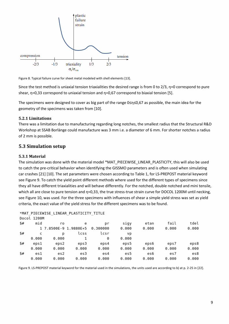
5.1 DOCOL 1200M DOCOL 1200M is martensitic cold rolled isotropic [18] steel and belongs in the high strength group, for
microstructure see Figure 7. It has despite its high strength good forming and welding capacity and is often used
as safety components in the automotive industry such as bumper reinforcements, door beams and seat tracks,
see Figure 1 on page 1. The mechanical properties of DOCOL 1200M is seen in Table 1 and the chemical
composition is seen in Table 2 [19]. Young’s modulus was achieved from tension test of the mini tensile
specimen and calculated according to Hooke´s generalized law in one dimension [12].
Table 1. Mechanical properties for DOCOL 1200M in transverse direction [18] [19]
Yield strength
Rp0,2 [MPa]
Tensile strength Rm [MPa]
Elongation A80
[%] Young´s modulus
E [GPa] Density
ρ [kg/m3] Poisson ratio ν
min min max min 199 7850 0,3 9501 1200 1400 3
Table 2. Chemical composition for DOCOL 1200M [19]
C % max
Si % max
Mn % max
P % max
S % max
Al % min
Nb+Ti % max
0,14 0,40 2,0 0,020 0,010 0,015 0,10
Figure 7. A cross section seen in a light microscope etched in 3% NItal [20].
The sheet provided by SSAB had a thickness of 1 mm and was leveled. The leveling process means that it has
been rolled an extra time in order to be more flat, this also gives some not evenly distributed plastic
deformations and some internal stresses.
5.2 Choice of specimens In order to make GISSMO as flexible as possible the range of experimentally achieved triaxialities should be as
big as possible [10]. According to LS-DYNA® Keyword User’s Manual Volume II [13] the triaxialities that can be
achieved with shell elements is reaching from -2/3 to 2/3, see Figure 8.
1 Guaranteed minimum by SSAB
9
Figure 8. Typical failure curve for sheet metal modeled with shell elements [13].
Since the test method is uniaxial tension triaxialities the desired range is from 0 to 2/3, η=0 correspond to pure
shear, η=0,33 correspond to uniaxial tension and η=0,67 correspond to biaxial tension [5].
The specimens were designed to cover as big part of the range 0≤η≤0,67 as possible, the main idea for the
geometry of the specimens was taken from [10].
5.2.1 Limitations
There was a limitation due to manufacturing regarding long notches, the smallest radius that the Structural R&D
Workshop at SSAB Borlänge could manufacture was 3 mm i.e. a diameter of 6 mm. For shorter notches a radius
of 2 mm is possible.
5.3 Simulation setup
5.3.1 Material
The simulation was done with the material model *MAT_PIECEWISE_LINEAR_PLASTICITY, this will also be used
to catch the pre-critical behavior when identifying the GISSMO parameters and is often used when simulating
car crashes [21] [10]. The set parameters were chosen according to Table 1, for LS-PREPOST material keyword
see Figure 9. To catch the yield point different methods where used for the different types of specimens since
they all have different triaxialities and will behave differently. For the notched, double notched and mini tensile,
which all are close to pure tension and η≈0,33, the true stress-true strain curve for DOCOL 1200M until necking,
see Figure 10, was used. For the three specimens with influences of shear a simple yield stress was set as yield
criteria, the exact value of the yield stress for the different specimens was to be found.
Figure 9. LS-PREPOST material keyword for the material used in the simulations, the units used are according to b) at p. 2-25 in [22].
10
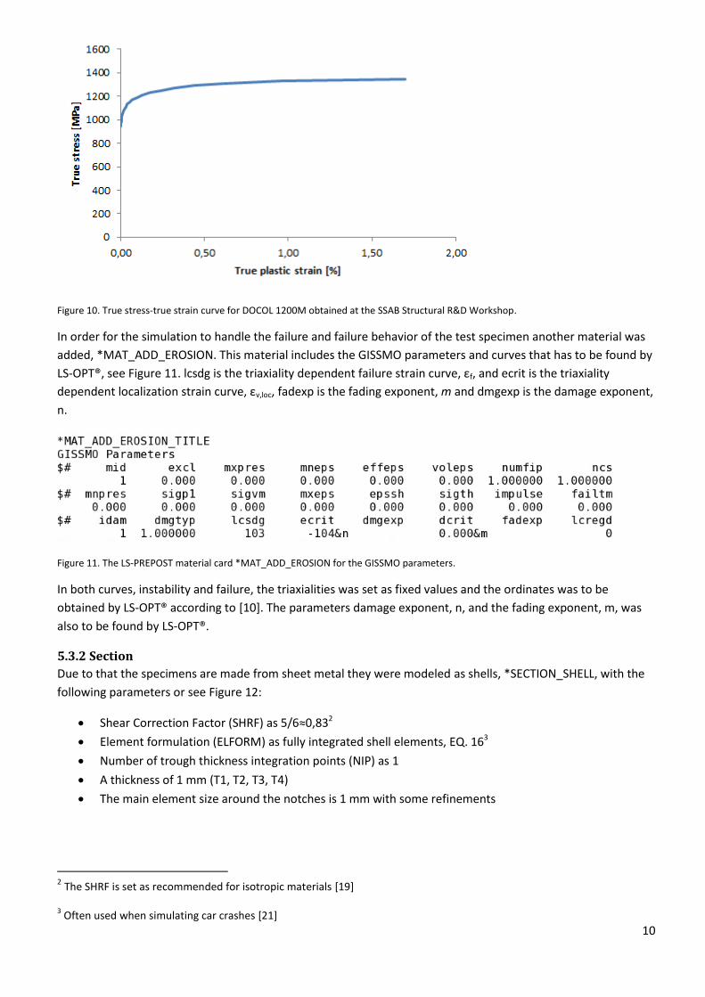
Figure 10. True stress-true strain curve for DOCOL 1200M obtained at the SSAB Structural R&D Workshop.
In order for the simulation to handle the failure and failure behavior of the test specimen another material was
added, *MAT_ADD_EROSION. This material includes the GISSMO parameters and curves that has to be found by
LS-OPT®, see Figure 11. lcsdg is the triaxiality dependent failure strain curve, εf, and ecrit is the triaxiality
dependent localization strain curve, εv,loc, fadexp is the fading exponent, m and dmgexp is the damage exponent,
n.
Figure 11. The LS-PREPOST material card *MAT_ADD_EROSION for the GISSMO parameters.
In both curves, instability and failure, the triaxialities was set as fixed values and the ordinates was to be
obtained by LS-OPT® according to [10]. The parameters damage exponent, n, and the fading exponent, m, was
also to be found by LS-OPT®.
5.3.2 Section
Due to that the specimens are made from sheet metal they were modeled as shells, *SECTION_SHELL, with the
following parameters or see Figure 12:
Shear Correction Factor (SHRF) as 5/6≈0,832
Element formulation (ELFORM) as fully integrated shell elements, EQ. 163
Number of trough thickness integration points (NIP) as 1
A thickness of 1 mm (T1, T2, T3, T4)
The main element size around the notches is 1 mm with some refinements
2 The SHRF is set as recommended for isotropic materials [19]
3 Often used when simulating car crashes [21]
11
Figure 12. LS-PREPOST section keyword for the section used in the simulations.
5.3.3 Boundary conditions (SPC) & displacement
The specimens were controlled by two sets of BCs, one at the bottom with all DOFs locked and one at the top
with all DOFs except translation in y-direction. The simulation was done with displacement control to imitate
the testing as much as possible. The displacement was set with the BC *BOUNDARY_PRESCRIBED_MOTION_SET
and was applied on a set of nodes at the top of the specimen. The scale factor was set in order to achieve the
displacement in the experiment, the displacement were applied with the curve seen in Figure 13.
Figure 13. Curve used to apply the displacement in LS-PREPOST.
In the experiment the specimens were run with a speed of 5 mm/min which gives a total time of 46 seconds for
the shear 0° specimen which had the biggest displacement. For time saving purposes the simulation was run on
1 second which for that specimen would give a speed of 228 mm/min. In this thesis the strain rate dependency
is assumed to be negligible, the assumption is based on Figure 14.
12
Figure 14. Stress strain curves for DOCOL 1200M for different speeds, the curve was achieved at the Structural R&D laboratory at SSAB Borlänge.
5.3.4 Force and displacement measurement
The displacement measurement was carried out by using the database keyword *HISTORY_NODE for two nodes
centered in x-direction located at equal distance from the center with 80 mm between, as the later used
extensometer. The force was measured by the database keyword *SECFORC and *CROSS_SECTION, it measures
the force in a specific cross section, the cross section is located in the thick part of the lower half of the
specimen.
5.3.5 Solver
The calculations where solved explicitly and to speed up the simulation the time step was increased with mass
scaling according to equation 14 [23], the density was increased 1000 times.
ELt
(14)
When mass scaling is used artificial inertia forces are added and needs to be treated very careful so that these
artificial inertia forces don’t dominate the global result [24]. It is assumed that the calculations are reliable if the
kinetic energy when the deformation has reached not negligible values is below ≈3%.
5.4 Specimens The specimens that were decided to be tested in the experiments in order to achieve good results for GISSMO
are seen in Figure 15. A more detailed view of the specimens can be seen in Appendix A. The simulated elastic
triaxiality for the different specimens is also seen in Figure 15 and shows a good distribution.
13
Figure 15. The six chosen specimens.
Out of these specimens five will be used to identify GISSMO parameters and a sixth, shear 60°, will be used for
validation of GISSMO.
5.5 Experimental
5.5.1 Manufacturing of specimens
The specimens were manufactured at the Structural R&D Workshop at SSAB Borlänge. First the specimens were
cut to course external dimensions from the sheet using a power shear. The specimens were cut in TD of the
sheet because that is the most usual test direction. In order to avoid possible differs in properties in the edge of
the sheet from manufacturing the specimens were cut close to the middle in TD. In order to keep track of the
specimens and to minimize the variations in properties in a set of specimens they were.
When the specimens were cut to their external dimensions the specimens were milled by a CNC milling machine
to their final shape.
Out of each specimen type six replicates were manufactured to get a good statistical basis and prevent that
outliers are being used in the parameter identification or validation.
5.5.2 Testing
The testing was done with a displacement controlled Zwick 100 uniaxial tension testing machine, the data of the
machine is seen in Table 3. According to the calibration report the error margins for measurement of force was
±0,12% at affected loads. The displacement was measured with an 80 mm extensometer in order to only read
the displacement in the test specimen and not the machine itself, as an example shear 45° is seen in Figure 16,
the error margins for the affected displacements was ±0,15% according to the calibration report.
14
Table 3. Test machine data
Machine Zwick 100 Displacement sensor 80 mm extensometer, Epsilon Load sensor Internal hydraulic load cell (ISO 7500-1 Class 0,5 from 1000 N to 100000 N) Test speed 5 mm/min Calibration date 2013-03-31 load cell, 2014-06-17 extensometer
Figure 16. Shear 45° specimen clamped in the uniaxial tension testing machine with attached extensometer.
5.6 Optimization The optimization was done using LS-OPT®, the parameters are set with an initial value and upper and lower
bounds then the software chooses the parameters for the different simulations. The metamodel used was the
feedforward neural network with space filling point selection as recommended in the LS-OPT® manual [14].
The objective for the optimization was to match the force displacement curves from the simulations with the
experimentally achieved curves with as small error as possible, this method usually gives a good match for this
types of tasks [15]. First the optimization was done for each case separate in order to make sure that the
models were good and to get good starting values for the last optimization, the flowchart for the optimization of
one case is seen in Figure 17. The mean value of the achieved parameters is be used as starting values for the
combined optimization.
15
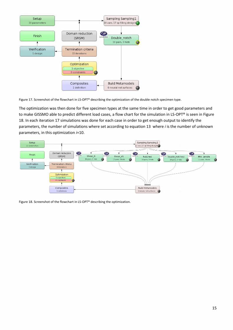
Figure 17. Screenshot of the flowchart in LS-OPT® describing the optimization of the double notch specimen type.
The optimization was then done for five specimen types at the same time in order to get good parameters and
to make GISSMO able to predict different load cases, a flow chart for the simulation in LS-OPT® is seen in Figure
18. In each iteration 17 simulations was done for each case in order to get enough output to identify the
parameters, the number of simulations where set according to equation 13 where i is the number of unknown
parameters, in this optimization i=10.
Figure 18. Screenshot of the flowchart in LS-OPT® describing the optimization.

16
5.7 Mesh size dependency Since the small dimensions of the specimen a quite small mesh size is used, ≈1 mm, due to calculation time
much coarser elements needs to be used on a full scale car crash simulation. On full scale car crash simulation
elements used had an average size up to 6-7 mm with a minimum size of 4mm is used [25]. In order to see how
the achieved parameters predict the failure with other element sizes the mini tensile specimen will be simulated
with different element sizes 1 mm, 2 mm and 4 mm. The different models will be simulated with the parameters
achieved with 1mm elements then regularization will be examined.
17
6 Results Since LS-OPT® only handles one target curve the achieved force displacement curves had to be reduced to one
for each case, for more details see Appendix B. For convergence plots of the parameters and optimizations see
Appendix C.
6.1 Single case parameter identifications
6.1.1 Shear 0°
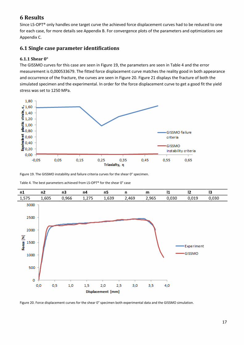
The GISSMO curves for this case are seen in Figure 19, the parameters are seen in Table 4 and the error
measurement is 0,000533679. The fitted force displacement curve matches the reality good in both appearance
and occurrence of the fracture, the curves are seen in Figure 20. Figure 21 displays the fracture of both the
simulated specimen and the experimental. In order for the force displacement curve to get a good fit the yield
stress was set to 1250 MPa.
Figure 19. The GISSMO instability and failure criteria curves for the shear 0° specimen.
Table 4. The best parameters achieved from LS-OPT® for the shear 0° case
n1 n2 n3 n4 n5 n m l1 l2 l3
1,575 1,605 0,966 1,275 1,639 2,469 2,965 0,030 0,019 0,030
Figure 20. Force displacement curves for the shear 0° specimen both experimental data and the GISSMO simulation.
18
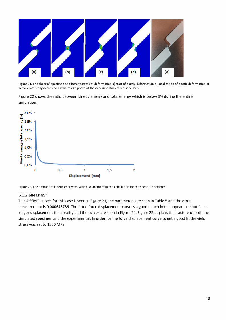
Figure 21. The shear 0° specimen at different states of deformation a) start of plastic deformation b) localization of plastic deformation c) heavily plastically deformed d) failure e) a photo of the experimentally failed specimen.
Figure 22 shows the ratio between kinetic energy and total energy which is below 3% during the entire
simulation.
Figure 22. The amount of kinetic energy vs. with displacement in the calculation for the shear 0° specimen.
6.1.2 Shear 45°
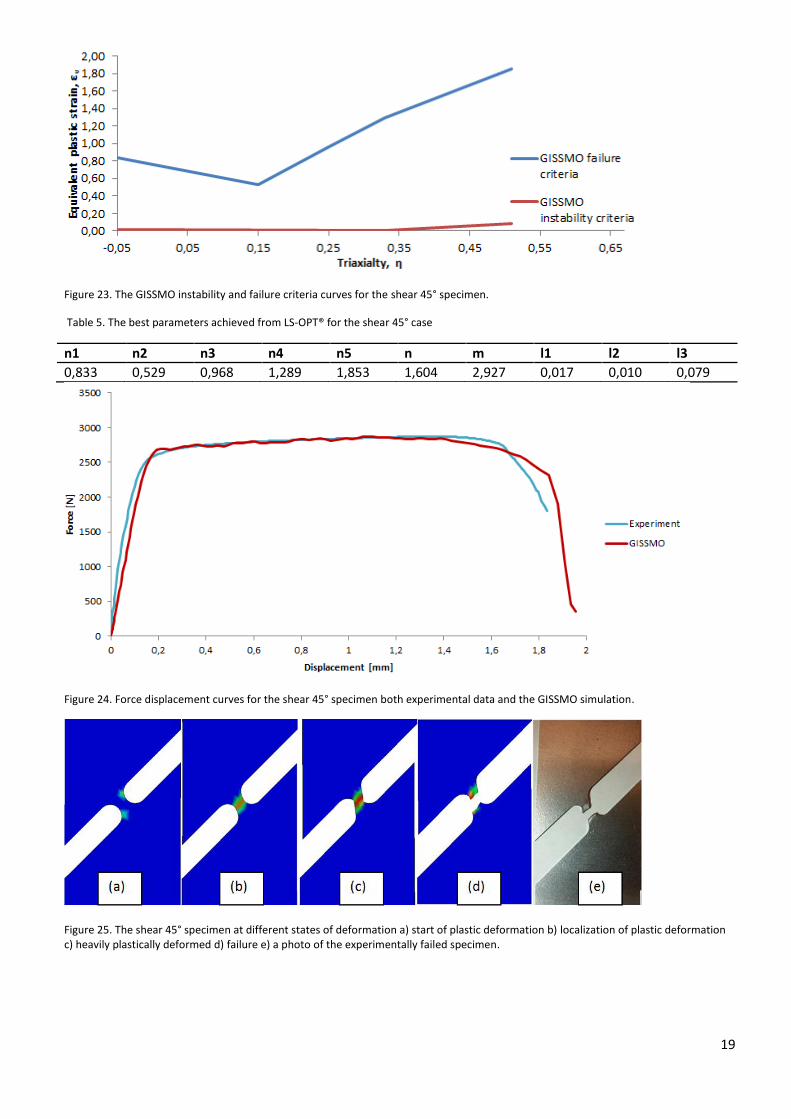
The GISSMO curves for this case is seen in Figure 23, the parameters are seen in Table 5 and the error
measurement is 0,000648786. The fitted force displacement curve is a good match in the appearance but fail at
longer displacement than reality and the curves are seen in Figure 24. Figure 25 displays the fracture of both the
simulated specimen and the experimental. In order for the force displacement curve to get a good fit the yield
stress was set to 1350 MPa.
19
Figure 23. The GISSMO instability and failure criteria curves for the shear 45° specimen.
Table 5. The best parameters achieved from LS-OPT® for the shear 45° case
n1 n2 n3 n4 n5 n m l1 l2 l3
0,833 0,529 0,968 1,289 1,853 1,604 2,927 0,017 0,010 0,079
Figure 24. Force displacement curves for the shear 45° specimen both experimental data and the GISSMO simulation.
Figure 25. The shear 45° specimen at different states of deformation a) start of plastic deformation b) localization of plastic deformation c) heavily plastically deformed d) failure e) a photo of the experimentally failed specimen.
20
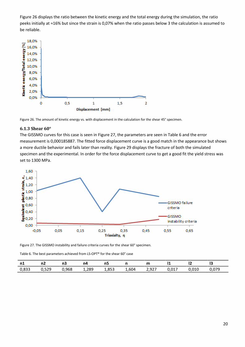
Figure 26 displays the ratio between the kinetic energy and the total energy during the simulation, the ratio
peeks initially at ≈16% but since the strain is 0,07% when the ratio passes below 3 the calculation is assumed to
be reliable.
Figure 26. The amount of kinetic energy vs. with displacement in the calculation for the shear 45° specimen.
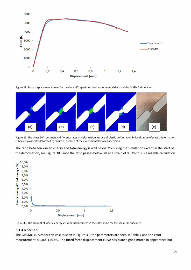
6.1.3 Shear 60°
The GISSMO curves for this case is seen in Figure 27, the parameters are seen in Table 6 and the error
measurement is 0,000185887. The fitted force displacement curve is a good match in the appearance but shows
a more ductile behavior and fails later than reality. Figure 29 displays the fracture of both the simulated
specimen and the experimental. In order for the force displacement curve to get a good fit the yield stress was
set to 1300 MPa.
Figure 27. The GISSMO instability and failure criteria curves for the shear 60° specimen.
Table 6. The best parameters achieved from LS-OPT® for the shear 60° case
n1 n2 n3 n4 n5 n m l1 l2 l3
0,833 0,529 0,968 1,289 1,853 1,604 2,927 0,017 0,010 0,079
21
Figure 28. Force displacement curves for the shear 60° specimen both experimental data and the GISSMO simulation.
Figure 29. The shear 60° specimen at different states of deformation a) start of plastic deformation b) localization of plastic deformation c) heavily plastically deformed d) failure e) a photo of the experimentally failed specimen.
The ratio between kinetic energy and total energy is well below 3% during the simulation except in the start of
the deformation, see Figure 30. Since the ratio passes below 3% at a strain of 0,03% this is a reliable calculation.
Figure 30. The amount of kinetic energy vs. with displacement in the calculation for the shear 60° specimen.
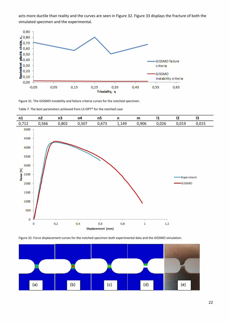
6.1.4 Notched
The GISSMO curves for this case is seen in Figure 31, the parameters are seen in Table 7 and the error
measurement is 0,000114069. The fitted force displacement curve has quite a good match in appearance but
22
acts more ductile than reality and the curves are seen in Figure 32. Figure 33 displays the fracture of both the
simulated specimen and the experimental.
Figure 31. The GISSMO instability and failure criteria curves for the notched specimen.
Table 7. The best parameters achieved from LS-OPT® for the notched case
n1 n2 n3 n4 n5 n m l1 l2 l3
0,712 0,566 0,802 0,507 0,673 1,149 0,906 0,026 0,019 0,015
Figure 32. Force displacement curves for the notched specimen both experimental data and the GISSMO simulation.
23
Figure 33. The notched specimen at different states of deformation a) start of plastic deformation b) localization of plastic deformation c) heavily plastically deformed d) failure e) a photo of the experimentally failed specimen.
The ratio between the kinetic energy and the total energy is below 3% during the entire simulation, see Figure
34.
Figure 34. The amount of kinetic energy vs. with displacement in the calculation for the notched specimen.
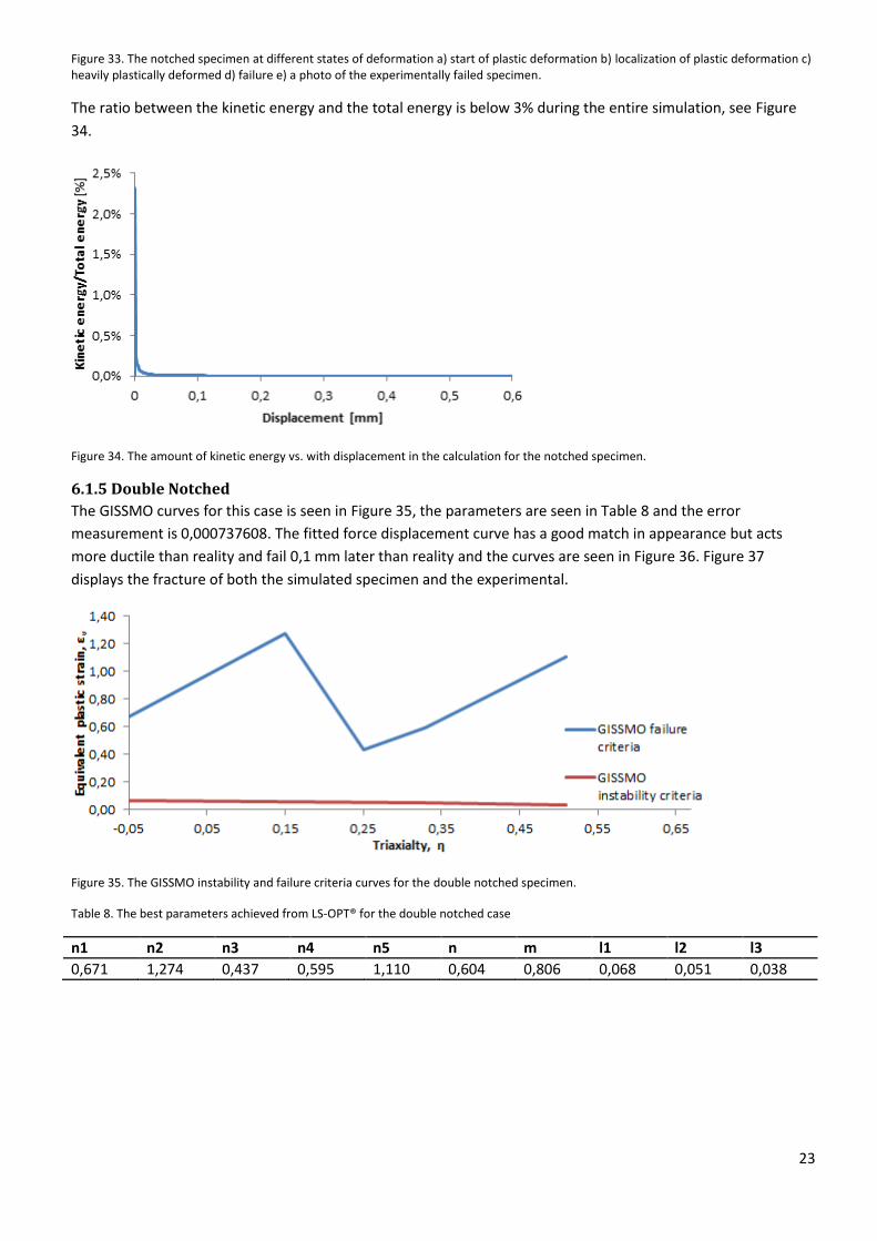
6.1.5 Double Notched
The GISSMO curves for this case is seen in Figure 35, the parameters are seen in Table 8 and the error
measurement is 0,000737608. The fitted force displacement curve has a good match in appearance but acts
more ductile than reality and fail 0,1 mm later than reality and the curves are seen in Figure 36. Figure 37
displays the fracture of both the simulated specimen and the experimental.
Figure 35. The GISSMO instability and failure criteria curves for the double notched specimen.
Table 8. The best parameters achieved from LS-OPT® for the double notched case
n1 n2 n3 n4 n5 n m l1 l2 l3
0,671 1,274 0,437 0,595 1,110 0,604 0,806 0,068 0,051 0,038
24
Figure 36. Force displacement curves for the double notched specimen both experimental data and the GISSMO simulation.
Figure 37. The double notched specimen at different states of deformation a) start of plastic deformation b) localization of plastic deformation c) heavily plastically deformed d) failure e) a photo of the experimentally failed specimen.
Figure 38 displays the ratio between the kinetic energy and the total energy that has a peek at 4,5% initially but
since the strain is 0,02% when the ratio passes below 3% the simulation is considered reliable.
Figure 38. The amount of kinetic energy vs. with displacement in the calculation for the double notched specimen.
6.1.6 Mini tensile
The GISSMO curves for this case is seen in Figure 39, the parameters are seen in Table 9 and the error
measurement is 0,000435789. The fitted force displacement curve catches the pre critical behavior good but
shows a more ductile fracture than reality and the curves are seen in Figure 40. Figure 41 displays the fracture of
both the simulated specimen and the experimental.
(a) (b)
25
Figure 39. The GISSMO instability and failure criteria curves for the mini tensile specimen.
Table 9. The best parameters achieved from LS-OPT® for the mini tensile case
n1 n2 n3 n4 n5 n m l1 l2 l3
0,475 0,250 0,225 0,201 0,379 2,622 0,678 0,034 0,018 0,026
Figure 40. Force displacement curves for the mini tensile specimen both experimental data and the GISSMO simulation.
26
Figure 41. The mini tensile specimen at different states of deformation a) start of plastic deformation b) localization of plastic deformation c) heavily plastically deformed d) failure e) a photo of the experimentally failed specimen
Figure 42 displays the ratio between the kinetic energy and the total energy which is below ≈1% which indicates
that the mass scaling won’t interfere with the result.
Figure 42. The amount of kinetic energy vs. with displacement in the calculation for the mini tensile specimen.
27
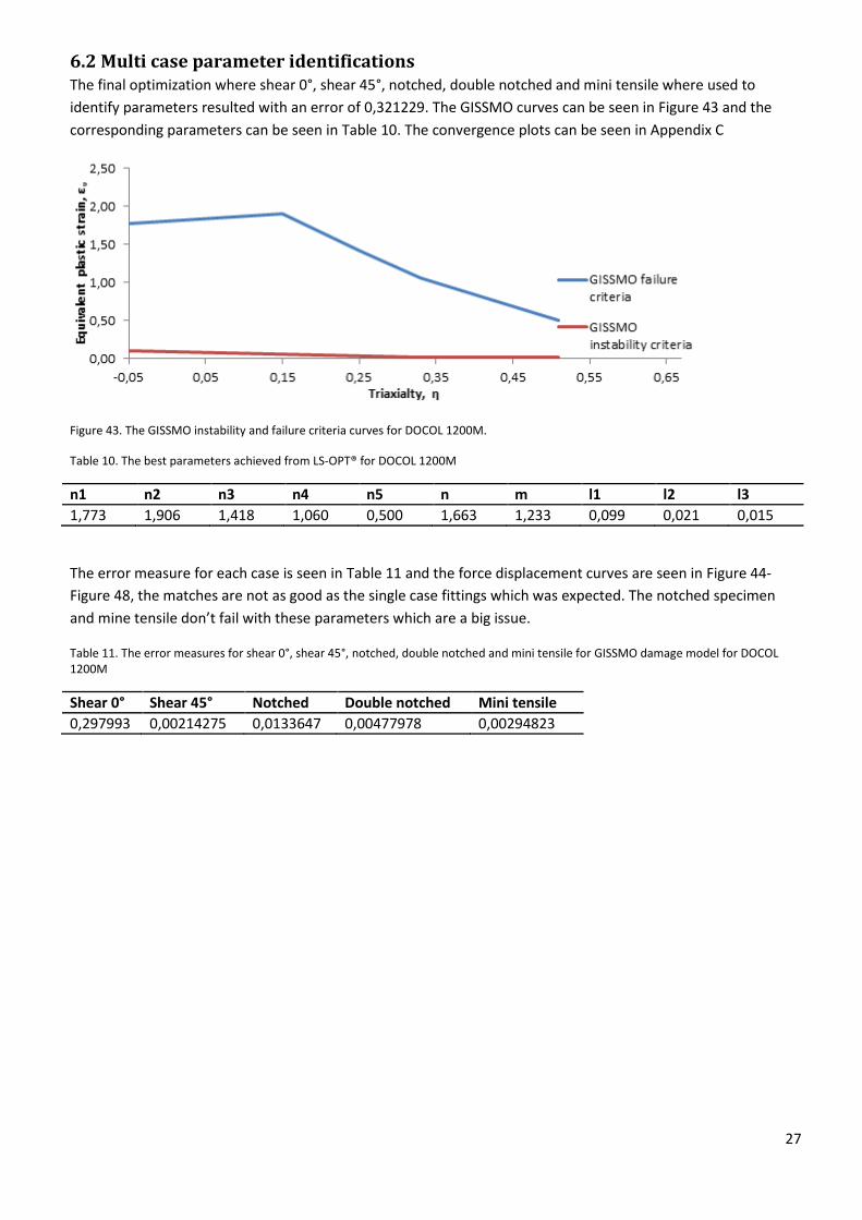
6.2 Multi case parameter identifications The final optimization where shear 0°, shear 45°, notched, double notched and mini tensile where used to
identify parameters resulted with an error of 0,321229. The GISSMO curves can be seen in Figure 43 and the
corresponding parameters can be seen in Table 10. The convergence plots can be seen in Appendix C
Figure 43. The GISSMO instability and failure criteria curves for DOCOL 1200M.
Table 10. The best parameters achieved from LS-OPT® for DOCOL 1200M
n1 n2 n3 n4 n5 n m l1 l2 l3
1,773 1,906 1,418 1,060 0,500 1,663 1,233 0,099 0,021 0,015
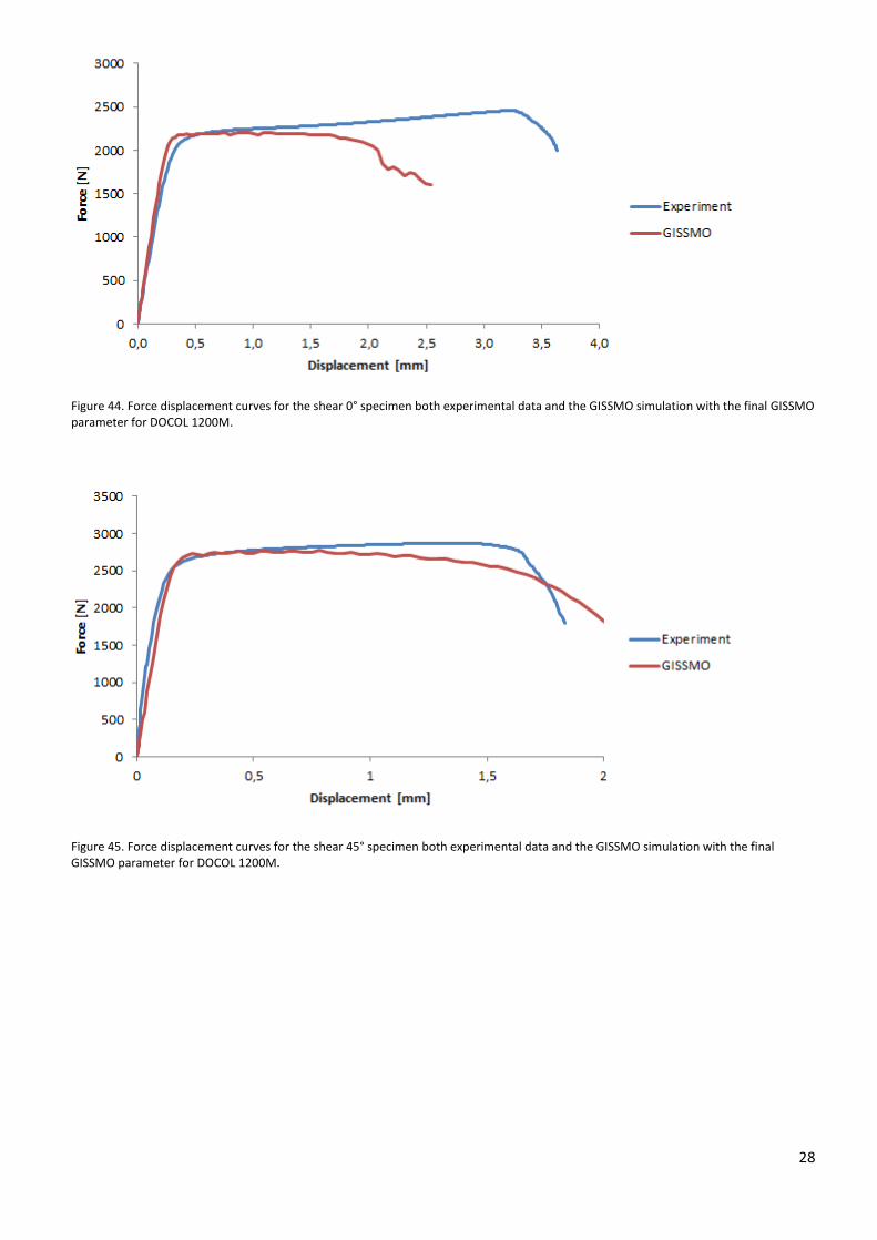
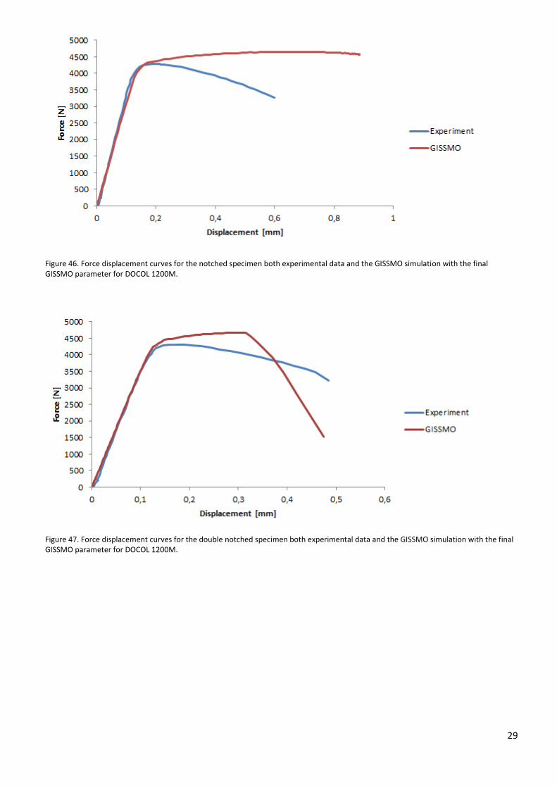
The error measure for each case is seen in Table 11 and the force displacement curves are seen in Figure 44-
Figure 48, the matches are not as good as the single case fittings which was expected. The notched specimen
and mine tensile don’t fail with these parameters which are a big issue.
Table 11. The error measures for shear 0°, shear 45°, notched, double notched and mini tensile for GISSMO damage model for DOCOL 1200M
Shear 0° Shear 45° Notched Double notched Mini tensile
0,297993 0,00214275 0,0133647 0,00477978 0,00294823
28
Figure 44. Force displacement curves for the shear 0° specimen both experimental data and the GISSMO simulation with the final GISSMO parameter for DOCOL 1200M.
Figure 45. Force displacement curves for the shear 45° specimen both experimental data and the GISSMO simulation with the final GISSMO parameter for DOCOL 1200M.
29
Figure 46. Force displacement curves for the notched specimen both experimental data and the GISSMO simulation with the final GISSMO parameter for DOCOL 1200M.
Figure 47. Force displacement curves for the double notched specimen both experimental data and the GISSMO simulation with the final GISSMO parameter for DOCOL 1200M.
30
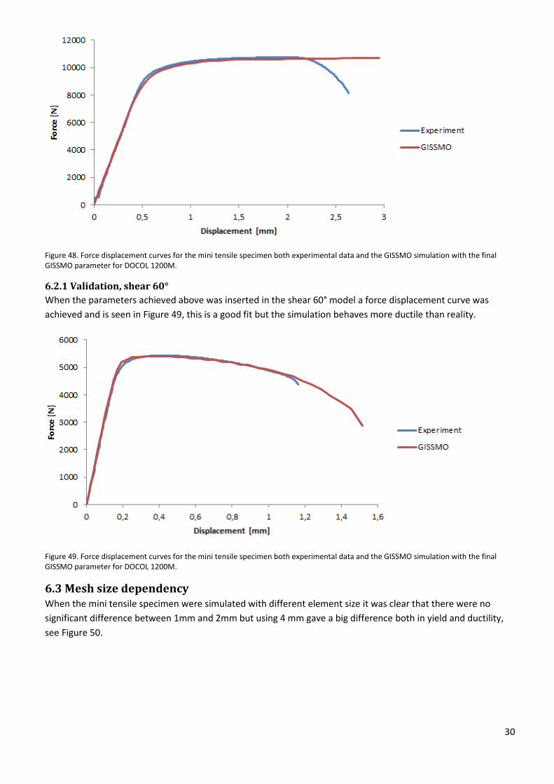
Figure 48. Force displacement curves for the mini tensile specimen both experimental data and the GISSMO simulation with the final GISSMO parameter for DOCOL 1200M.
6.2.1 Validation, shear 60°
When the parameters achieved above was inserted in the shear 60° model a force displacement curve was
achieved and is seen in Figure 49, this is a good fit but the simulation behaves more ductile than reality.
Figure 49. Force displacement curves for the mini tensile specimen both experimental data and the GISSMO simulation with the final GISSMO parameter for DOCOL 1200M.
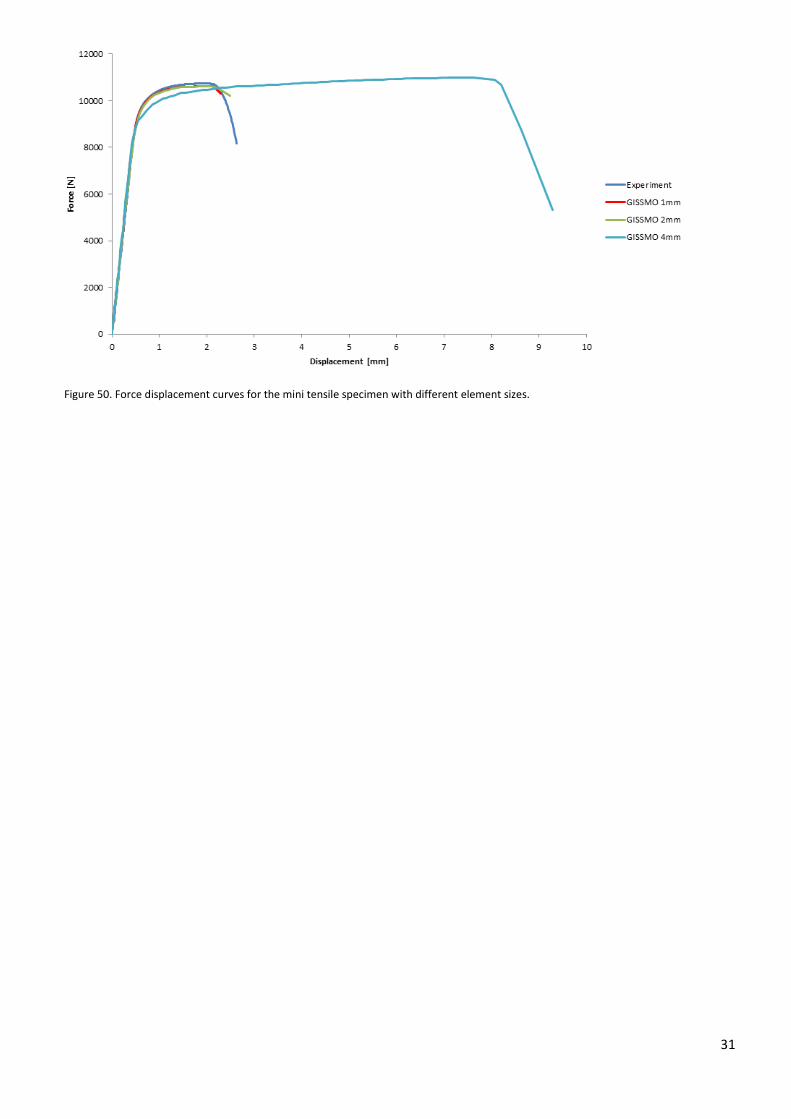
6.3 Mesh size dependency When the mini tensile specimen were simulated with different element size it was clear that there were no
significant difference between 1mm and 2mm but using 4 mm gave a big difference both in yield and ductility,
see Figure 50.
31
Figure 50. Force displacement curves for the mini tensile specimen with different element sizes.
32
7 Discussion Without having heard about GISSMO or triaxiality before I dove into this project it was much reading articles in
the beginning, the articles was not that detailed since most of them was contributions to the LS-DYNA® Users
conference of different editions. Something that I had to get started with really quick before I really had
understood the theory was specimen design. I’m satisfied with the achieved distribution in triaxiality but the
small dimensions of the specimens gave a need for a fine mesh and in full car crash simulations there is a need
for big elements to decrease calculation time.
In order to get a good match for the shear specimens different yield stresses had to be used, this is a bit
concerning but not inexplicably since they have different triaxialities and if the instability and failure differs the
yield might as well have different values for different stress states.
At first the force displacement curves was achieved with the internal displacement sensor but that sensor also
registered gaps in the machine which resulted in some bad really strange curves. I worked with the curves for a
couple of weeks before I decided to manufacture new specimens and testing them with an extensometer
instead which gave considerable more reliable results.
The error was measured with the area between the curves which is essentially the height times the length of the
curve so a longer curve will generate a bigger error for the same amount of mismatch. There is an option in LS-
OPT® to give the different curve mappings different priorities (weights), if the priorities would have been scaled
according to the length of the experimental curve the optimization might have given a more equal result
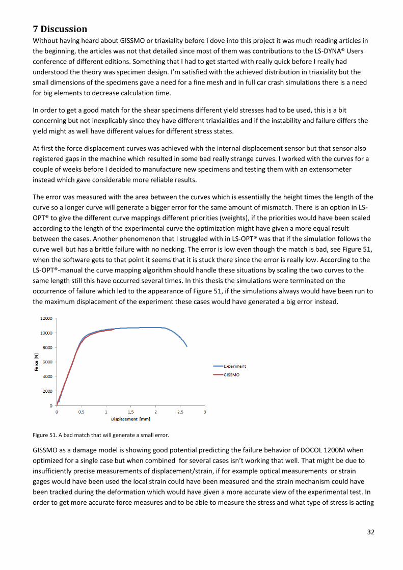
between the cases. Another phenomenon that I struggled with in LS-OPT® was that if the simulation follows the
curve well but has a brittle failure with no necking. The error is low even though the match is bad, see Figure 51,
when the software gets to that point it seems that it is stuck there since the error is really low. According to the
LS-OPT®-manual the curve mapping algorithm should handle these situations by scaling the two curves to the
same length still this have occurred several times. In this thesis the simulations were terminated on the
occurrence of failure which led to the appearance of Figure 51, if the simulations always would have been run to
the maximum displacement of the experiment these cases would have generated a big error instead.
Figure 51. A bad match that will generate a small error.
GISSMO as a damage model is showing good potential predicting the failure behavior of DOCOL 1200M when
optimized for a single case but when combined for several cases isn’t working that well. That might be due to
insufficiently precise measurements of displacement/strain, if for example optical measurements or strain
gages would have been used the local strain could have been measured and the strain mechanism could have
been tracked during the deformation which would have given a more accurate view of the experimental test. In
order to get more accurate force measures and to be able to measure the stress and what type of stress is acting

33
at the moment load cells could have been used. Unfortunately neither load cells nor strain gages/optical
measurments was available during this project.
Since each optimization for the multi case took more or less a week there was no time to let them continue for
more iterations but that would probably improve the result since the parameters haven’t converged to its final
value, see section C.7 Multi case.
7.1 Error sources Since there is a RD and a TD in the steel sheet there are some amount of anisotropy and since this sheet are also
leveled in RD that could increase that effect.
7.2 Future work In order to improve this model the experiments could be done using optical measurments/strain gages and load
cells to get more accurate local stress and strain measures.
To make the GISSMO model to work for a wider range of stress states a pure shear test, such as a butterfly
specimen, could be used and also compressive tests could be involved to cover the negative triaxialities for
sheet metals, see Figure 8.
In order to make the parameters to converge more it would be necessary to let the optimization run for more
iterations.
GISSMO offers the possibility to adjust with respect to element size by scaling the fading exponent and the
failure criteria curve, this need to be investigated in order to make GISSMO work for the automotive industry
where larger elements are used. This would also increase the accuracy of these simulations since all elements
are not exactly 1mm.
8 Conclusion The thesis was aimed to find the fading exponent, damage exponent and the instability- and failure curve for the
damage model to be able to catch the failure behavior of DOCOL 1200M which was done. The result was on the
other hand a bit unsatisfying because although the behavior of the validation specimen, shear 60°, was
predicted good except showing some more ductility than reality the other specimens was not that well matched.
When the specimens were optimized individually there was a good fit for all specimens which imply that there is
potential to find the parameters in order to have a good fit. Based on the ability of GISSMO damage model to
predict the failure behavior in the individual cases I believe that GISSMO is a good model for failure criteria but it
needs some more time to find the correct parameters in order to be able to use in crashworthiness simulations.

34
9 Acknowledgements I would like to thank Knowledge Service Center at SSAB Borlänge and my supervisor Nima Asadi Rad, MSc, for his
knowledge in crashworthiness simulations. I also want to thank the lab technicians at the Structural R&D
workshop for helpful tips regarding specimen design and providing of test data. I would like to specially thank
Jan Andersson for help with manufacturing of specimens and Anders Rosvall for helping me with testing. David
Aspenberg, PhD, at Dynamore Nordic with helpful tips with LS-DYNA. I also want to thank my supervisor at the
university Anders Gåård, PhD, for his valuable tips during the project. At last I would like to thank my fiancé
Josefine Montelius, BSc, for her support and good discussions during the project.
35
10 References
[1] H. L. Maclean and L. B. Lave, "Life cycle assessment of automobile/fuel options," Environmental Science &
Technology, vol. 37, no. 23, pp. 5445-5452, 2003.
[2] D. Schultz and A. Abraham, "North American light vehicle material trends," in Great designs in steel, Livonia,
2009.
[3] A. Sandahl, "Crash CAE in the all new Volvo XC90 & SPA platform," in Nordic LS-DYNA® Users Forum,
Gothenburg, 2014.
[4] T. Löfgren, Stålboken, Borlänge: SSAB Informationsavdelningen, 2009.
[5] F. Neukamm, M. Feucht and A. Haufe, "Consistent Damage Modelling in the Process Chain of Forming to
Crashworthiness Simulations," in LS-DYNA® Anwenderforum, Bamberg, 2008.
[6] Mercedes-Benz, "Mercedes-Benz introduces the safety body," August 1959. [Online]. Available:
http://www.mercedesclass.net/safety-2/safety-technology/august-1959-mercedes-benz-introduces-the-
safety-body/. [Accessed 24 March 2015].
[7] T. Gholami, J. Lescheticky and R. Paßmann, "Crashworthiness Simulation of Automobiles with
ABAQUS/Explicit," in 2003 ABAQUS User's Conference, Munich, 2003.
[8] P. Gudmundson, "11 Damage Mechanics," in Material Mechanics, Stockholm, Department of Solid
Mechanics, KTH Engineering Sciences, 2006, pp. 193-202.
[9] J. Lemaitre, "A Continuous Damage Mechanics," Journal of Engineering Materials and Technology, vol. 107,
pp. 83-89, 1985.
[10] J. Effelsberg, A. Haufe, M. Feucht, F. Neukamm and P. Du Bois, "On parameter identification for the GISSMO
damage model," in 12th International LS-DYNA® Users Conference, Dearborn, 2012.
[11] F. Neukamm, M. Feucht and A. Haufe, "Considering damage history in crashworthiness simulations," in 7th
European LS-DYNA® Conference, Salzburg, 2009.
[12] B. Sundström, Handbok och formelsamling i Hållfasthetslära, Stockholm: Institutionen för hållfasthetslära
KTH, 2008.
[13] LSTC, "LS-DYNA® Keyword User's Manual Volume II-Material Models," 26 May 2014. [Online]. Available:
http://www.dynasupport.com/manuals/ls-dyna-manuals/ls-dyna-manual-r-7.1-vol-i. [Accessed 28 January
2015].
[14] N. Stander, W. Roux, A. Basudhar, T. Eggleston, T. Goel and K. Craig, "LS-OPT® User´s Manual A design
optimization and probalistic analysis tool for the engineering analyst," June 2014. [Online]. Available:
http://www.lsoptsupport.com/documents/manuals. [Accessed 4 March 2015].
[15] K. Witowski, M. Feucht and N. Stander, "An Effective Curve Matching Metric for Parameter Identification
using Partial Mapping," in 8th European LS-DYNA® Users Conference, Strasbourg, 2011.
36
[16] I. R. Santos and P. S. Santos, "Simulation metamodels for modelling output distribution parameters,"
Technical University of Lisbon, Lisbon, 2007.
[17] N. Stander, W. Roux, M. Giger, M. Redhe, N. Fedorova and J. Haarhoff, "Crashworthiness Optimization in
LSOPT: Case Studies in Metamodelling and Random Search Techniques," in 4th European LS-DYNA® Users
Conference, Ulm, 2003.
[18] J. Kuoppa, J. Samuelsson, J.-O. Sperle, L. Rydahl, E. Pétursson, J. Larsson, J. Gozzi, M. Gustafsson, L. Bäckman,
M. Reinberth, T. Nilsson, P. Alm, L. Troive, A. Ivarsson, P.-E. Augustsson, P. Alm and J. Eckerlid, "2 Ståltyper
och deras egenskaper," in Plåthandboken Att konstruera och tillverka i höghållfast stål, Borlänge, SSAB,
2012, pp. 2:1-2:7.
[19] SSAB, "Data Sheet 8251en Docol," 24 06 2014. [Online]. Available:
http://www.ssab.com/Global/DOCOL/datasheets_docol/en/251_Docol%201200%20M.pdf?epslanguage=en.
[Accessed 3 February 2015].
[20] C. Andersson, "Laboratorierapport N6.95CA.15.0093," SSAB, FoU, Metallografi, Borlänge, 2015.
[21] F. Andrade, M. Feucht and A. Haufe, "On the Prediction of Material Failure in LS-DYNA®: A Comparison
Between GISSMO and DIEM," in 13th International LS-DYNA® Users Conference, Dearborn, 2014.
[22] LSTC, "LS-DYNA® Keyword User's Manual Volume I," 26 May 2014. [Online]. Available:
http://www.dynasupport.com/manuals/ls-dyna-manuals/ls-dyna-manual-r-7.1-vol-i. [Accessed 2 February
2015].
[23] DYNAmore, "LS-DYNA® Support," DYNAmore, April 2010. [Online]. Available:
http://www.dynasupport.com/howtos/general/selective-mass-scaling-sms-2. [Accessed 25 March 2015].
[24] L. Olovsson, K. Simonsson and M. Unosson, "Selective mass scaling for explicit finite element analyses,"
International Journal For Numerical Methods In Engineering, vol. 63, pp. 1436-1445, 2005.
[25] D. Mazougui, D. Brown, H. Park, C. Kan and K. Opiela, "Development & Validation of a Finite Element Model
for a Mid-Sized Passenger Sedan," in 13th International LS-DYNA® Users Conference, Dearborn, 2014.
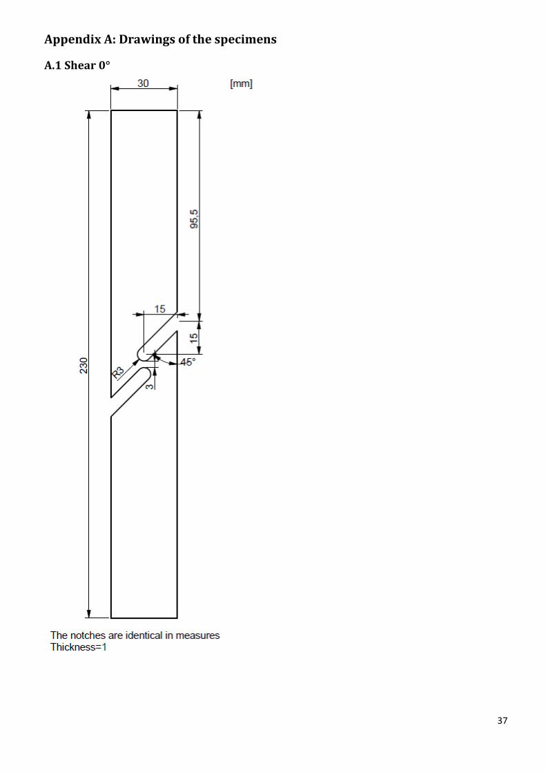
37
Appendix A: Drawings of the specimens
A.1 Shear 0°
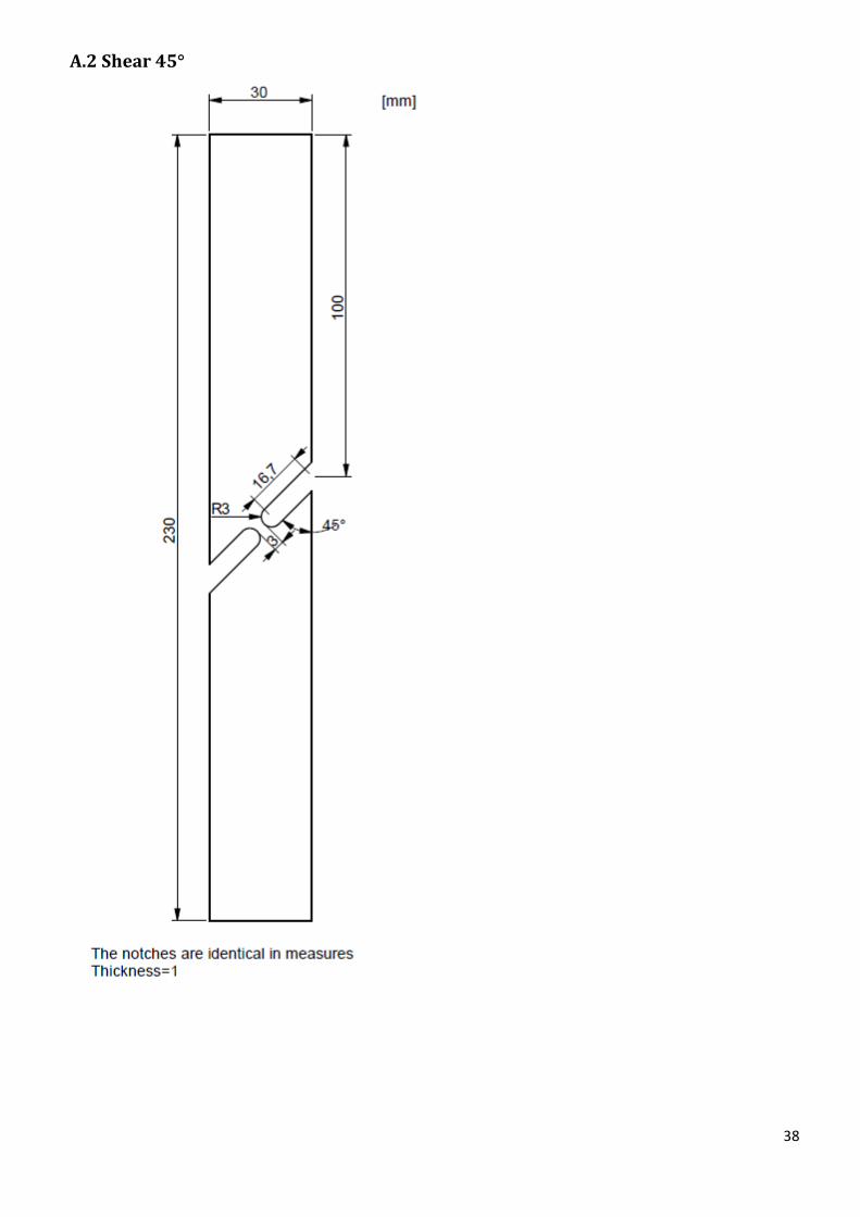
38
A.2 Shear 45°
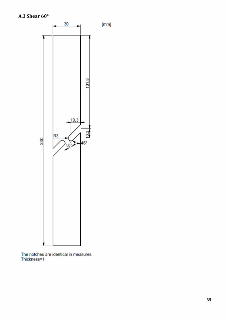
39
A.3 Shear 60°
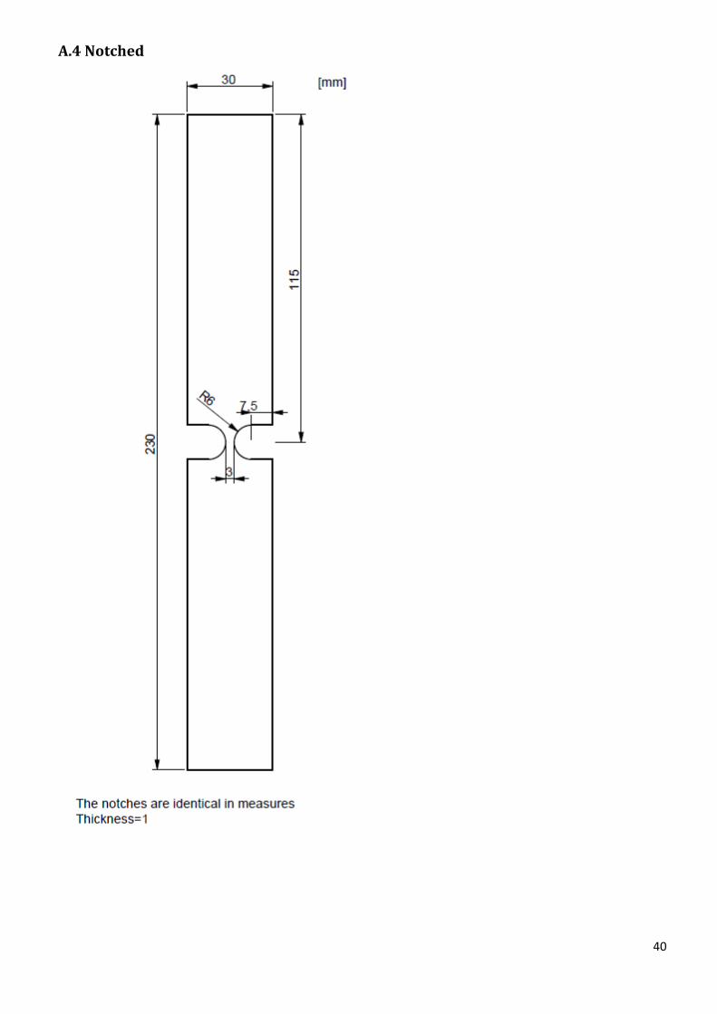
40
A.4 Notched
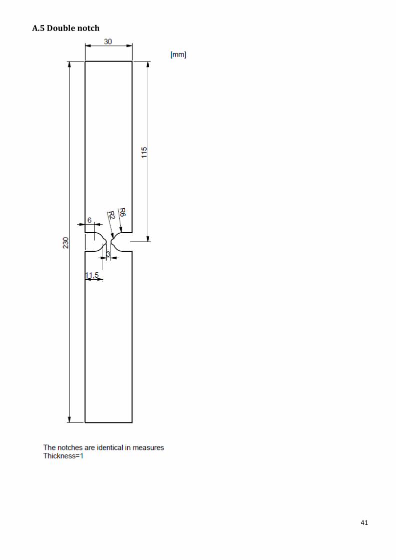
41
A.5 Double notch
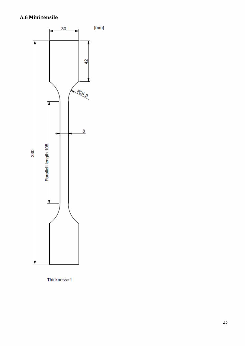
42
A.6 Mini tensile
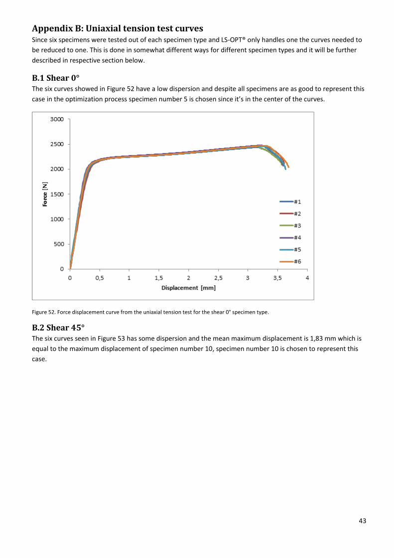
43
Appendix B: Uniaxial tension test curves Since six specimens were tested out of each specimen type and LS-OPT® only handles one the curves needed to
be reduced to one. This is done in somewhat different ways for different specimen types and it will be further
described in respective section below.
B.1 Shear 0° The six curves showed in Figure 52 have a low dispersion and despite all specimens are as good to represent this
case in the optimization process specimen number 5 is chosen since it’s in the center of the curves.
Figure 52. Force displacement curve from the uniaxial tension test for the shear 0° specimen type.
B.2 Shear 45° The six curves seen in Figure 53 has some dispersion and the mean maximum displacement is 1,83 mm which is
equal to the maximum displacement of specimen number 10, specimen number 10 is chosen to represent this
case.
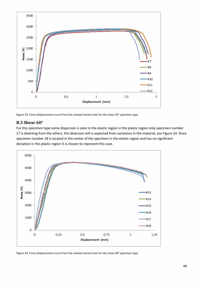
44
Figure 53. Force displacement curve from the uniaxial tension test for the shear 45° specimen type.
B.3 Shear 60° For this specimen type some dispersion is seen in the elastic region in the plastic region only specimen number
17 is diverting from the others, this diversion still is expected from variations in the material, see Figure 54. Since
specimen number 18 is located in the center of the specimen in the elastic region and has no significant
deviation in the plastic region it is chosen to represent this case.
Figure 54. Force displacement curve from the uniaxial tension test for the shear 60° specimen type.
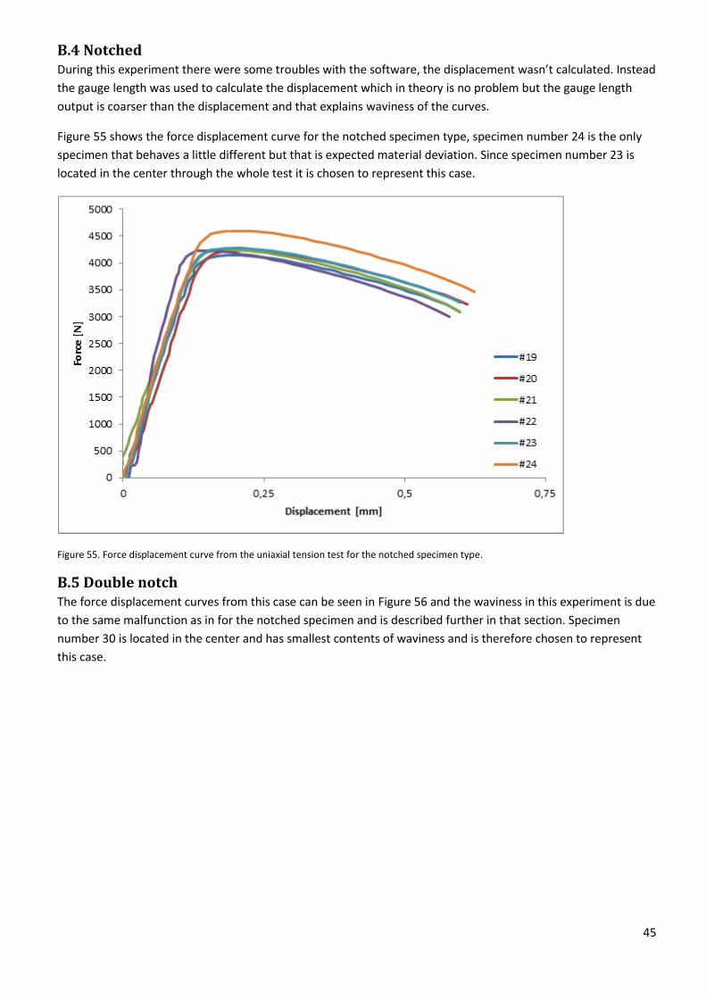
45
B.4 Notched During this experiment there were some troubles with the software, the displacement wasn’t calculated. Instead
the gauge length was used to calculate the displacement which in theory is no problem but the gauge length
output is coarser than the displacement and that explains waviness of the curves.
Figure 55 shows the force displacement curve for the notched specimen type, specimen number 24 is the only
specimen that behaves a little different but that is expected material deviation. Since specimen number 23 is
located in the center through the whole test it is chosen to represent this case.
Figure 55. Force displacement curve from the uniaxial tension test for the notched specimen type.
B.5 Double notch The force displacement curves from this case can be seen in Figure 56 and the waviness in this experiment is due
to the same malfunction as in for the notched specimen and is described further in that section. Specimen
number 30 is located in the center and has smallest contents of waviness and is therefore chosen to represent
this case.
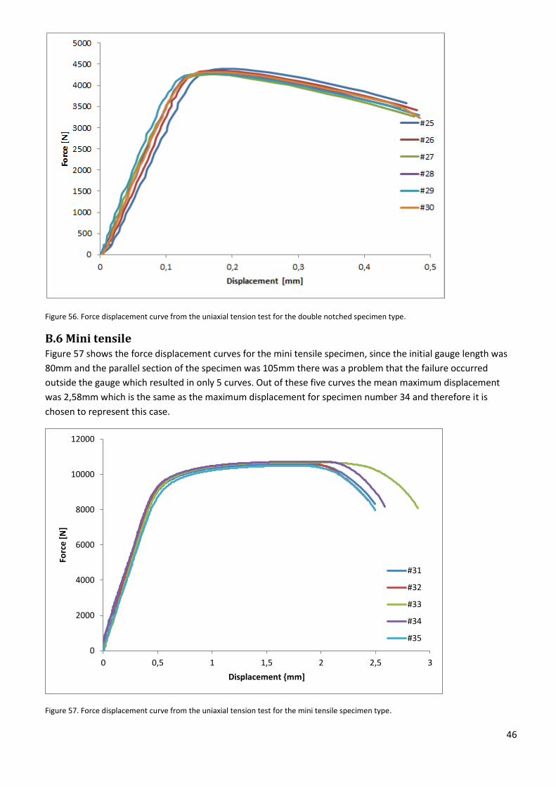
46
Figure 56. Force displacement curve from the uniaxial tension test for the double notched specimen type.
B.6 Mini tensile Figure 57 shows the force displacement curves for the mini tensile specimen, since the initial gauge length was
80mm and the parallel section of the specimen was 105mm there was a problem that the failure occurred
outside the gauge which resulted in only 5 curves. Out of these five curves the mean maximum displacement
was 2,58mm which is the same as the maximum displacement for specimen number 34 and therefore it is
chosen to represent this case.
Figure 57. Force displacement curve from the uniaxial tension test for the mini tensile specimen type.
0
2000
4000
6000
8000
10000
12000
0 0,5 1 1,5 2 2,5 3
Forc
e [
N]
Displacement {mm]
#31
#32
#33
#34
#35
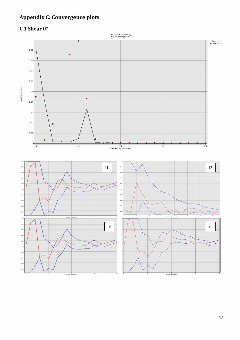
47
Appendix C: Convergence plots
C.1 Shear 0°
l1
l3
l2
m
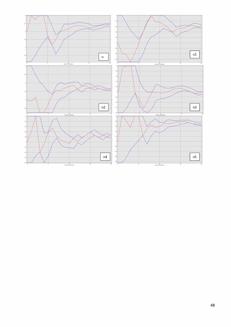
48
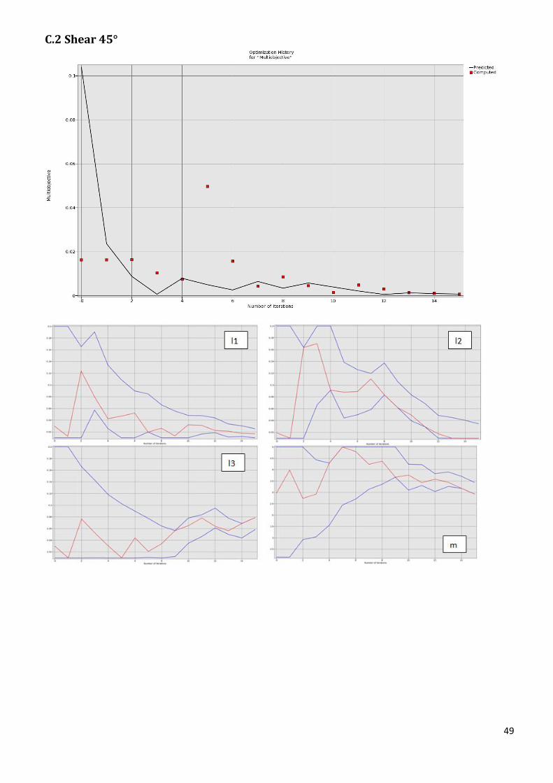
49
C.2 Shear 45°
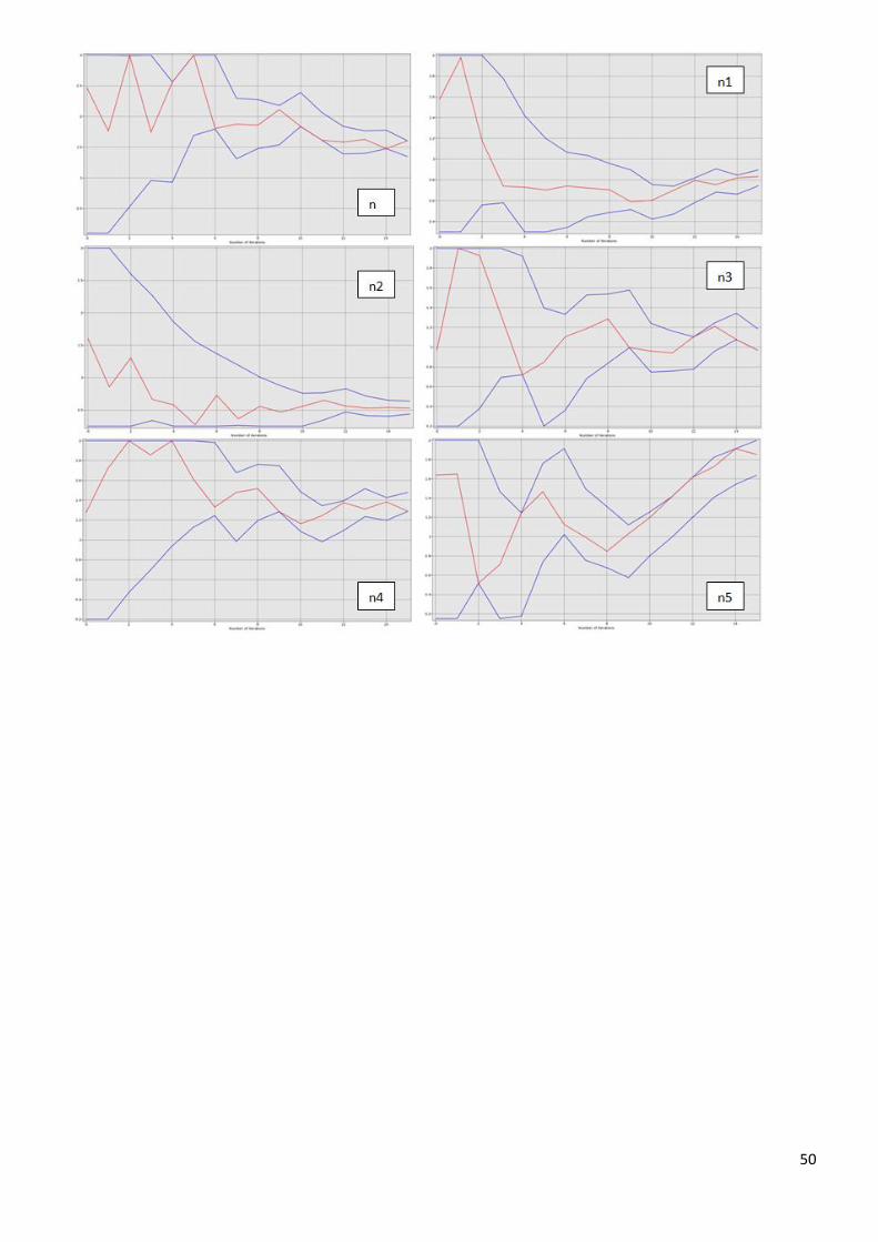
50
l1 l2
l3
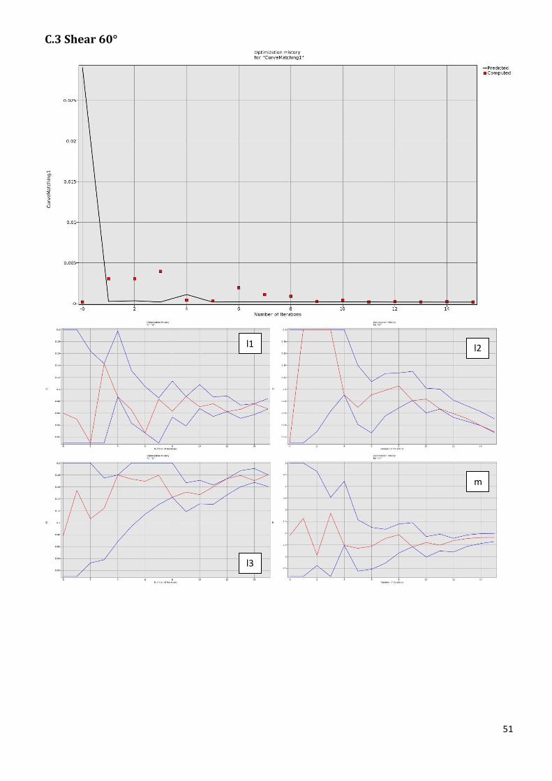
51
C.3 Shear 60°
l1 l2
l3
m
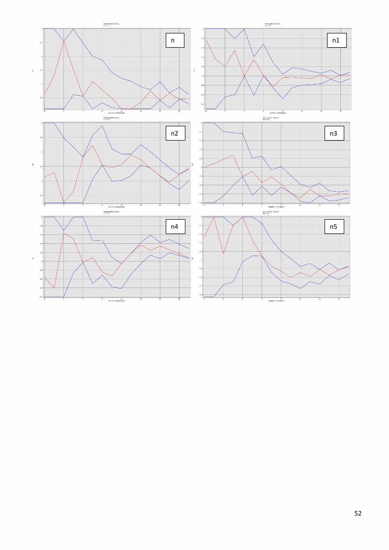
52
n n1
n2 n3
n4 n5
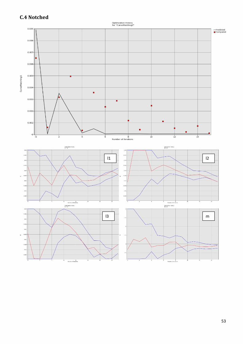
53
C.4 Notched
l1 l2
l3 m
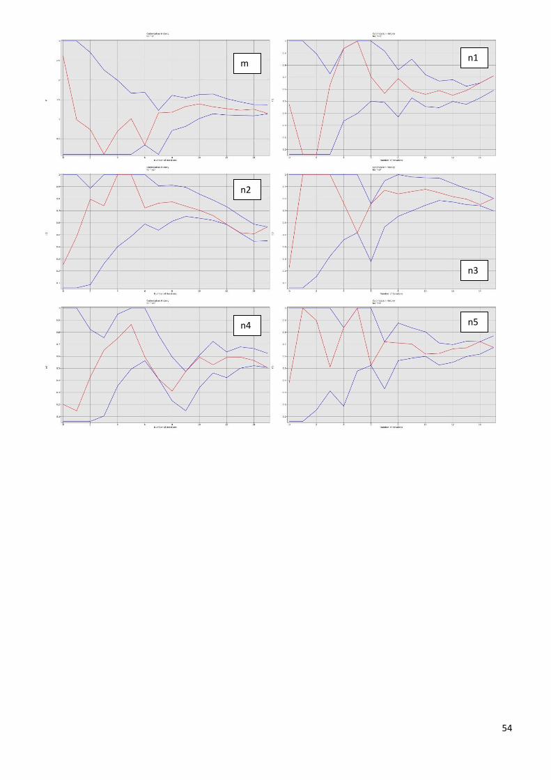
54
m n1
n2
n3
n4 n5
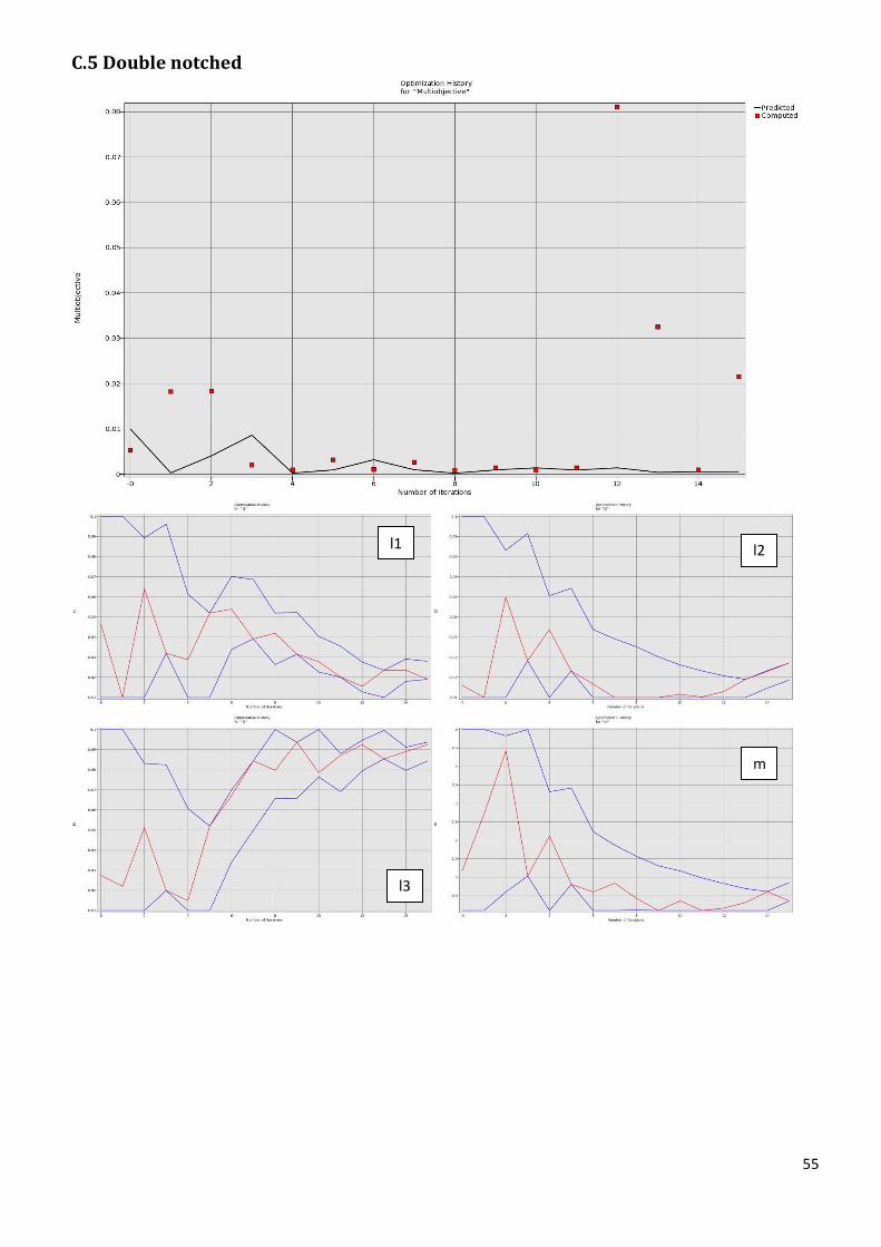
55
C.5 Double notched
l1 l2
l3
m
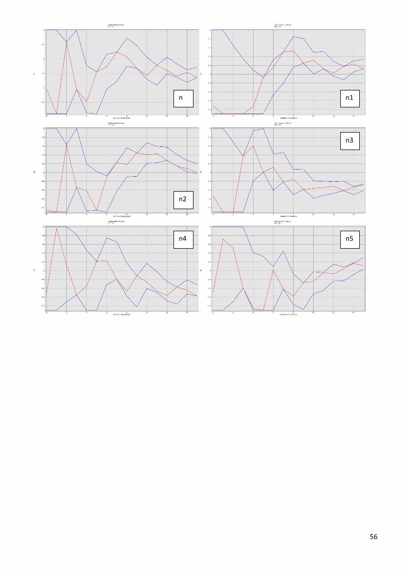
56
n1 n
n2
n3
n4 n5
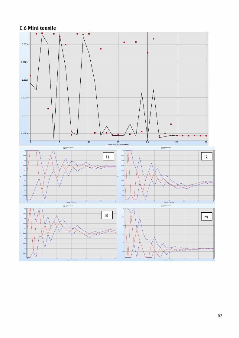
57
C.6 Mini tensile
l1 l2
l3 m
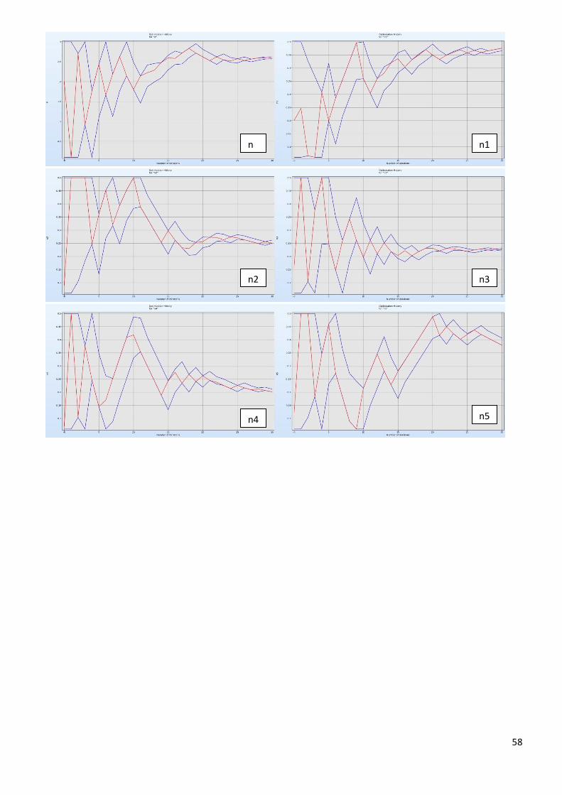
58
n n1
n2 n3
n4 n5
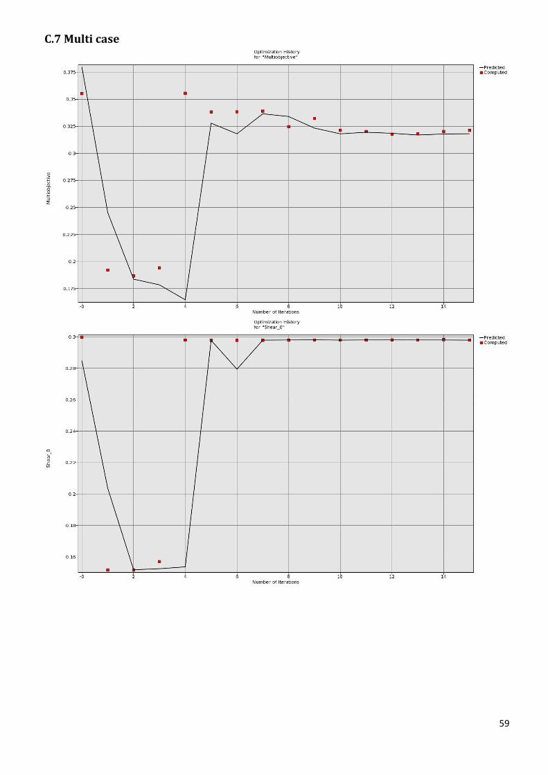
59
C.7 Multi case
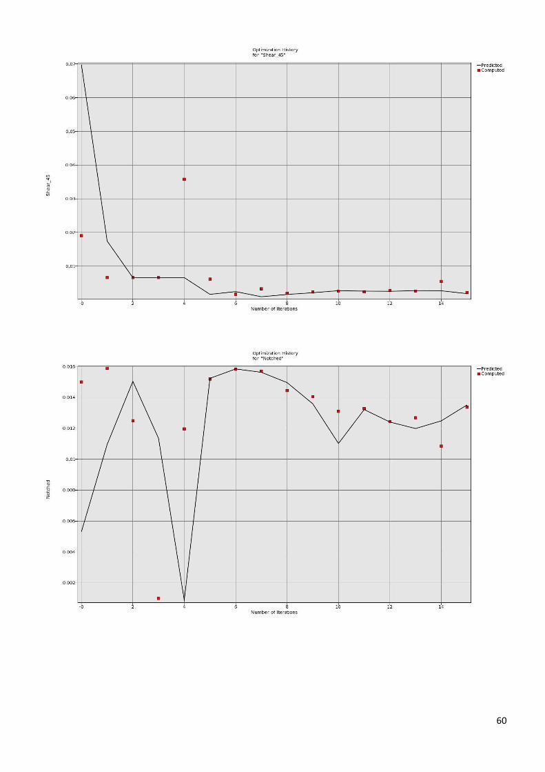
60
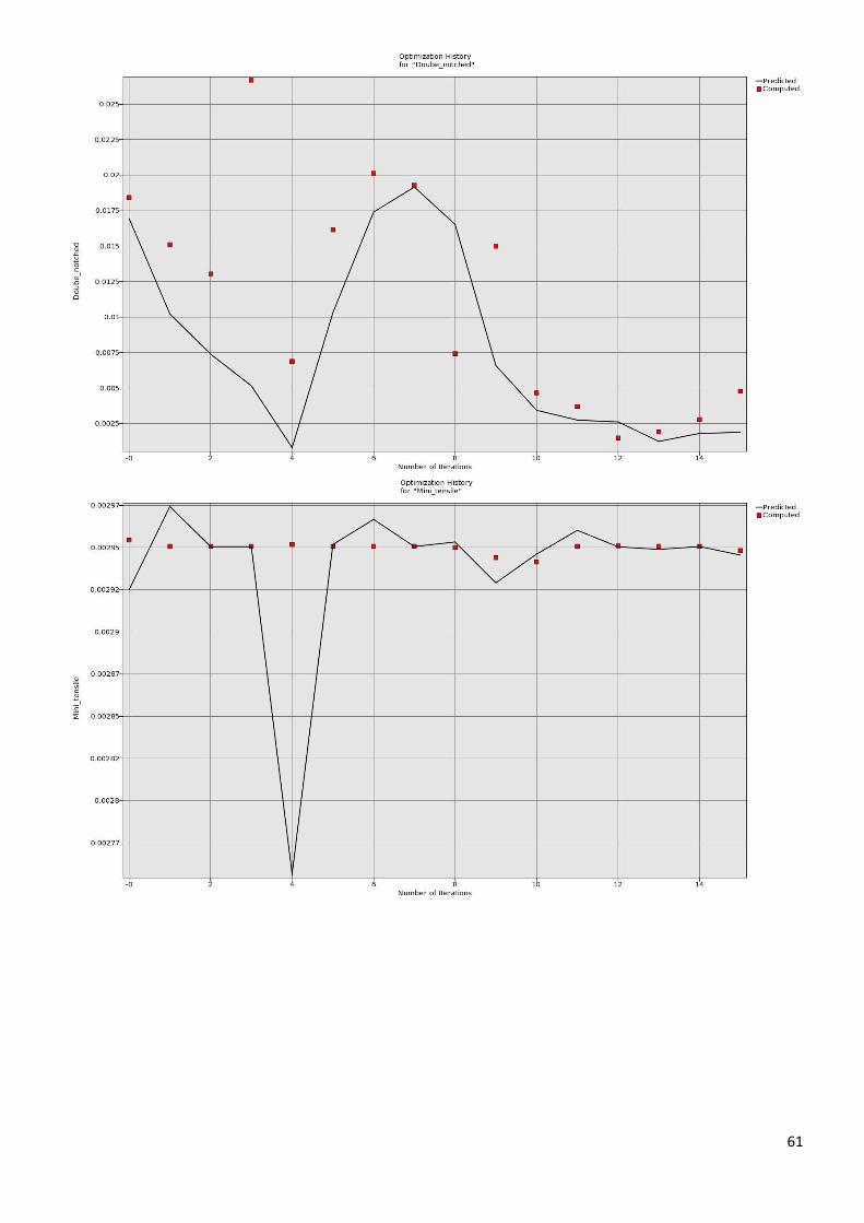
61
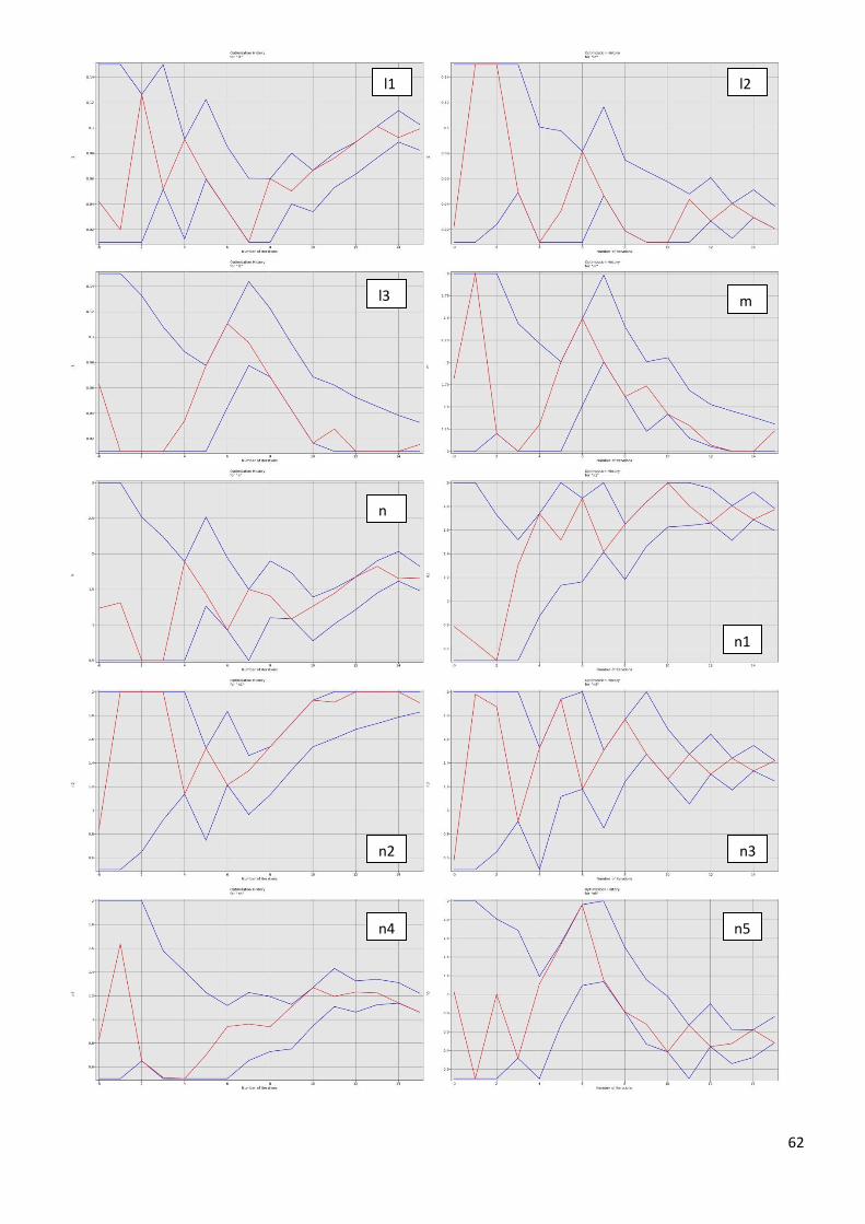
62
l1 l2
l3 m
n
n1
n2 n3
n4 n5