Parallel two-step Runge-Kutta methods - hu-berlin.degaggle/EVENTS/2006/BRENT60... · Parallel...
30
Parallel two-step Runge-Kutta methods Helmut Podhaisky, [email protected] Martin–Luther–University Halle–Wittenberg, Germany 20 July 2006
-
Upload
vuonghuong -
Category
Documents
-
view
217 -
download
0
Transcript of Parallel two-step Runge-Kutta methods - hu-berlin.degaggle/EVENTS/2006/BRENT60... · Parallel...

Parallel two-step Runge-Kutta methods
Helmut Podhaisky, [email protected]
Martin–Luther–University Halle–Wittenberg, Germany
20 July 2006

Outline
Runge–Kutta and multi-step methods
Explicit parallel peer methods
Implicit parallel peer methods
Summary

Explicit Runge–Kutta methods for y ′ = f (y)
classical Runge–Kutta method (1904)
Ym1 = ym−1
Ym2 = ym−1 +1
2hf (Ym1)
Ym3 = ym−1 +1
2hf (Ym2)
Ym4 = ym−1 + hf (Ym3)
ym = ym−1 +h
6f (Ym1) +
h
3f (Ym2) +
h
3f (Ym3) +
h
6f (Ym4)

Explicit Runge–Kutta methods for y ′ = f (y)
classical Runge–Kutta method (1904)
Ym1 = ym−1
Ym2 = ym−1 +1
2hf (Ym1)
Ym3 = ym−1 +1
2hf (Ym2)
Ym4 = ym−1 + hf (Ym3)
ym = ym−1 +h
6f (Ym1) +
h
3f (Ym2) +
h
3f (Ym3) +
h
6f (Ym4)
Butcher scheme
0
12
12
12 0 1
2
1 0 0 1
16
13
13
16
◮ the computation is sequential
◮ Ymk is not an accurate approximation to y(tm−1 + ckh)leading to complex order conditions
◮ linear stability can be studied easily
◮ stepsize changes are trivial

Explicit Runge–Kutta methods, Dormand/Prince (1980)
order 5, much better accuracy than RK4
0
15
15
310
340
940
45
4445 −56
15329
89
193726561 −25360
2187644486561 −212
729
1 90173168 −355
33467325247
49176 − 5103
18656
1 35384 0 500
1113125192 −2187
67841184
35384 0 500
1113125192 −2187
67841184
◮ widely used, Matlab: ode45
◮ not parallelizable

Bashforth and Adams (1883)
explicit multistep methods, e.g. order 4:
y [m] = y [m−1] +h
24(55fm−1 − 59fm−2 + 37fm−3 − 9fm−4)
◮ the computation in sequential
◮ the order conditions are rather simple, just interpolation
◮ linear stability is more difficult to analyze
◮ implementing a robust variable stepsize–variable order code isquite a challenge, Matlab ode113

Implicit methods
Runge–Kutta methods
◮ low stage order =⇒ orderreduction
◮ high stage order =⇒coupled iterations (and agood chance for someparallelization, bottleneck:LU-decomposition of theJacobian)
Multistep methods
◮ second Dahlquist barrier: anA-stable method cannothave order p > 2
◮ not parallelizable
Questions:
◮ What limitations can be overcome with more generalmethods? In particular: what about parallelism?
◮ Is it possible to be competitive in applications?

Explicit parallel peer methods
Idea: re-use stages from the last step
Ym =
Ym1
Ym2
...
Yms
, Ymk = y(tm + ckh) + O(hp+1)
Scheme: A and B full s × s matrices
Ym = hAf (Ym−1) + BYm−1
◮ the computation is completely parallel
◮ the order conditions are simple as long as p ≤ s − 1(interpolation, B = B(A))
◮ we want zero-stability with no parasitic roots, σ(B) = {1, 0}
◮ difficult: optimizing stability and variable stepsize behaviour

order conditions for Ym = hAf (Ym−1) + BYm−1
Taylor series expansion
With z = h ddt
, we have Ym = exp(cz)y(tm) and
exp(cz) = Az exp((c − 1)z) + B exp((c − 1)z) + O(zp+1)
which can be satisfied for B easily if p = s − 1.

order conditions for Ym = hAf (Ym−1) + BYm−1
Taylor series expansion
With z = h ddt
, we have Ym = exp(cz)y(tm) and
exp(cz) = Az exp((c − 1)z) + B exp((c − 1)z) + O(zp+1)
which can be satisfied for B easily if p = s − 1.ordered by powers of z
exp(cz) ∼
1 c1c212 . . .
cs−11
s−1!
1 c2c222 . . .
cs−12
s−1!...
...... . . .
...
1 csc2s
2 . . . cs−1s
s−1!

order conditions for Ym = hAf (Ym−1) + BYm−1
Taylor series expansion
With z = h ddt
, we have Ym = exp(cz)y(tm) and
exp(cz) = Az exp((c − 1)z) + B exp((c − 1)z) + O(zp+1)
which can be satisfied for B easily if p = s − 1.ordered by powers of z
exp((c − 1)z) ∼
1 c1 − 1(c−1)21
2 . . . (c1−1)s−1
s−1!
1 c2 − 1(c−1)22
2 . . . (c2−1)s−1
s−1!...
...... . . .
...
1 cs − 1 (c−1)2s2 . . . (cs−1)s−1
s−1!

order conditions for Ym = hAf (Ym−1) + BYm−1
Taylor series expansion
With z = h ddt
, we have Ym = exp(cz)y(tm) and
exp(cz) = Az exp((c − 1)z) + B exp((c − 1)z) + O(zp+1)
which can be satisfied for B easily if p = s − 1.ordered by powers of z
z exp((c − 1)z) ∼
0 1 c1 − 1 . . . (c1−1)s−2
s−2!
0 1 c2 − 1 . . . (c2−1)s−2
s−2!...
...... . . .
...
0 1 cs − 1 . . . (cs−1)s−2
s−2!

Explicit parallel peer methods, linear stability
Let y ′ = λy and z = hλ.We obtain
Ym = M(z)Ym−1 = (B + zA)Ym−1
◮ M(z) is called stability or amplification matrix.
◮ zero stability: B = M(0) must be power-bounded
◮ stability domain: {z : M(z) is power-bounded}

Explicit parallel peer methods, linear stability
Let y ′ = λy and z = hλ.We obtain
Ym = M(z)Ym−1 = (B + zA)Ym−1
◮ M(z) is called stability or amplification matrix.
◮ zero stability: B = M(0) must be power-bounded
◮ stability domain: {z : M(z) is power-bounded}
◮ example s = 6
−2 −1.5 −1 −0.5 0−1
−0.8
−0.6
−0.4
−0.2
0
0.2
0.4
0.6
0.8
1 compute boundary:M(z)v = exp(φi)vleads togeneralized EV problem:zA = (exp(φi)I − B)v

Explicit parallel peer methods, optimization
inner loop: linear conditions
◮ order p ≤ s − 1
◮ zero-parasitic eigenvalues: Schur-form QT B̂Q ist strictlyupper triangular,Q = (I + S)(I − S)−1 Cayley-transform, S – free skew matrix
◮ linear least squares, e.g. ‖A‖F and ‖B‖F
outer loop: nonlinear conditions
◮ ρ(M(z)), shape of the stability domain
◮ higher order errors p ≥ s, super-convergence conditions
After all, the method has to be reformulated for variable stepsizes.
⇒ work in progress

implicit parallel peer methods

Implicit parallel peer methods
parallel+implicit
Ymi depends on hf (Ymi )
Ym = Ghf (Ym) + hAf (Ym−1) + BYm−1, G = diag(g1, . . . , gs)
stiff accuracy
M(z) = (I − zG )−1(zA + B) vanishes for z → −∞ iff A = 0
example: method PP3, 3 stages, order 2
L-stable, stiffly accuratec = (−0.1, 0.7, 1), G = diag(1.7, 0.2670, 0.4454)
parasitic roots: B =
−0.21 6.79 −5.57
0.27 −2.46 3.18
0.31 −2.99 3.68
,
σ(B) = {1,−0.0005 ± 0.2202i} (for constant stepsize)

Implementation
◮ one Newton iteration per stage, linearly implicit method
◮ Krylov subspace K := span{b, Tb, . . . ,Tκ−1}, with T = fyFind x̄ for (I − γhT )x = b with x̄ ∈ K and (Ax̄ − b) ⊥ K.
◮ Fortran 90 using OpenMP for loop parallelization
◮ experiments on a SunFire (shared memory)
◮ spatial discretizations with finite differences and finitevolumes, respectively

Example 1: Diffu, ut = uxx + uyy + f (t, x , y)
with 0 ≤ t, x , y ≤ 1 and exact solutionsin(πx) sin(πy)(1 + 4xy sin t)
101
102
−8
−7.5
−7
−6.5
−6
−5.5
−5
−4.5
−4
−3.5
−3
−2.5
computing time (seconds)
log(
err)
VODPK
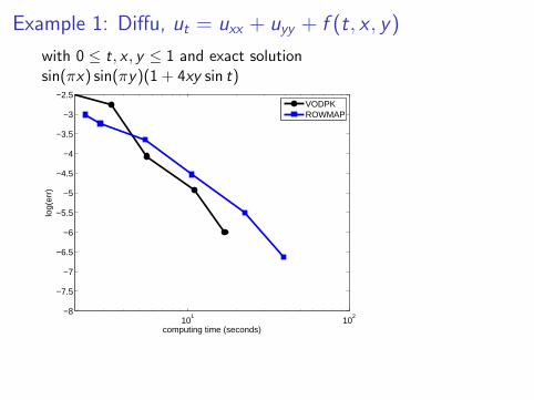
Example 1: Diffu, ut = uxx + uyy + f (t, x , y)
with 0 ≤ t, x , y ≤ 1 and exact solutionsin(πx) sin(πy)(1 + 4xy sin t)
101
102
−8
−7.5
−7
−6.5
−6
−5.5
−5
−4.5
−4
−3.5
−3
−2.5
computing time (seconds)
log(
err)
VODPKROWMAP

Example 1: Diffu, ut = uxx + uyy + f (t, x , y)
with 0 ≤ t, x , y ≤ 1 and exact solutionsin(πx) sin(πy)(1 + 4xy sin t)
101
102
−8
−7.5
−7
−6.5
−6
−5.5
−5
−4.5
−4
−3.5
−3
−2.5
computing time (seconds)
log(
err)
VODPKROWMAPPP3 (1 CPU)

Example 1: Diffu, ut = uxx + uyy + f (t, x , y)
with 0 ≤ t, x , y ≤ 1 and exact solutionsin(πx) sin(πy)(1 + 4xy sin t)
101
102
−8
−7.5
−7
−6.5
−6
−5.5
−5
−4.5
−4
−3.5
−3
−2.5
computing time (seconds)
log(
err)
VODPKROWMAPPP3 (1 CPU)PP3 (3 CPUs)

Example 2: Radiation-Diffusion
Mousseau, Knoll & Rider (2000), Verwer, Hundsdorfer (2003)
Et = ∇ · (Dr∇E ) + σ(T 4 − E ), Dr = (3σ + (1/E )|∂E/∂x |)−1,
Tt = ∇ · (Dt∇T ) − σ(T 4 − E ), Dt= kT 5/2, k = 0 or k = 0.1
strongly nonlinear, conservative second-order discretization
101
102
−5.5
−5
−4.5
−4
−3.5
−3
−2.5
−2
−1.5
−1
computing time (seconds)
log(
err)
VODPK

Example 2: Radiation-Diffusion
Mousseau, Knoll & Rider (2000), Verwer, Hundsdorfer (2003)
Et = ∇ · (Dr∇E ) + σ(T 4 − E ), Dr = (3σ + (1/E )|∂E/∂x |)−1,
Tt = ∇ · (Dt∇T ) − σ(T 4 − E ), Dt= kT 5/2, k = 0 or k = 0.1
strongly nonlinear, conservative second-order discretization
101
102
−5.5
−5
−4.5
−4
−3.5
−3
−2.5
−2
−1.5
−1
computing time (seconds)
log(
err)
VODPKROWMAP

Example 2: Radiation-Diffusion
Mousseau, Knoll & Rider (2000), Verwer, Hundsdorfer (2003)
Et = ∇ · (Dr∇E ) + σ(T 4 − E ), Dr = (3σ + (1/E )|∂E/∂x |)−1,
Tt = ∇ · (Dt∇T ) − σ(T 4 − E ), Dt= kT 5/2, k = 0 or k = 0.1
strongly nonlinear, conservative second-order discretization
101
102
−5.5
−5
−4.5
−4
−3.5
−3
−2.5
−2
−1.5
−1
computing time (seconds)
log(
err)
VODPKROWMAPPP3 (1 CPU)

Example 2: Radiation-Diffusion
Mousseau, Knoll & Rider (2000), Verwer, Hundsdorfer (2003)
Et = ∇ · (Dr∇E ) + σ(T 4 − E ), Dr = (3σ + (1/E )|∂E/∂x |)−1,
Tt = ∇ · (Dt∇T ) − σ(T 4 − E ), Dt= kT 5/2, k = 0 or k = 0.1
strongly nonlinear, conservative second-order discretization
101
102
−5.5
−5
−4.5
−4
−3.5
−3
−2.5
−2
−1.5
−1
computing time (seconds)
log(
err)
VODPKROWMAPPP3 (1 CPU)PP3 (2.5 cheated)

Summary
◮ classical methods cannot be parallelized, we need multi-stage,multi-step methods
◮ methods with parallel stages scale can be implemented easilyon shared memory computers (with, say, 2 to 8 CPUs/cores)
◮ order conditions can be satisfied by interpolation, however,super-convergence is more difficult to achieve
◮ the main difficulty lies in finding robust methods with smallcoefficients and moderate error constants
◮ sequential general linear methods are worth to be studied, too
John Butcher (NZ), Adrian Hill (UK),Caren Tischendorf (Matheon/Colone),group in Halle, . . .