Parallel Recursive Filtering of Infinite Input...
55
Parallel Recursive Filtering of Infinite Input Extensions Diego Nehab André Maximo IMPA GE Global Research GTC 2017
Transcript of Parallel Recursive Filtering of Infinite Input...

Parallel Recursive Filtering of Infinite Input Extensions
Diego Nehab André Maximo
IMPA GE Global Research
GTC 2017

Linear time-invariant filters
filter

Linear
• Invariant to scale
filter
scale
filter
scale

Linear
• Invariant to addition
addadd
filter
filter
filter

Time invariant
• Invariant to shift
filtert t
shift
filter
t
t t
shift
t

Convolution
• The convolution of sequences 𝐛 and 𝐡 is a sequence 𝐚
𝐚 = 𝐛 ∗ 𝐡 𝑎𝑖 =
𝑗=−∞
∞
𝑏𝑗ℎ𝑖−𝑗𝐛, 𝐡, 𝐚: ℤ → ℝ
𝐛
𝐡 𝐡 𝐡
𝐚 = 𝐛 ∗ 𝐡
𝐡

Linear shift-invariant filters are convolutions
filter’s impulse response
unit impulse
filter
convolve filter

∗
Examples
∗
∗

Outline of talk
• Introduction• Recursive filters are very useful
• Initialization at the boundaries is an important problem
• Exact recursive filtering of infinite input extensions• Closed-form formulas available for the first time
• Enable simple and effective algorithms
• Parallelization• Fastest recursive filtering algorithms to date
• First to filter infinite extensions exactly
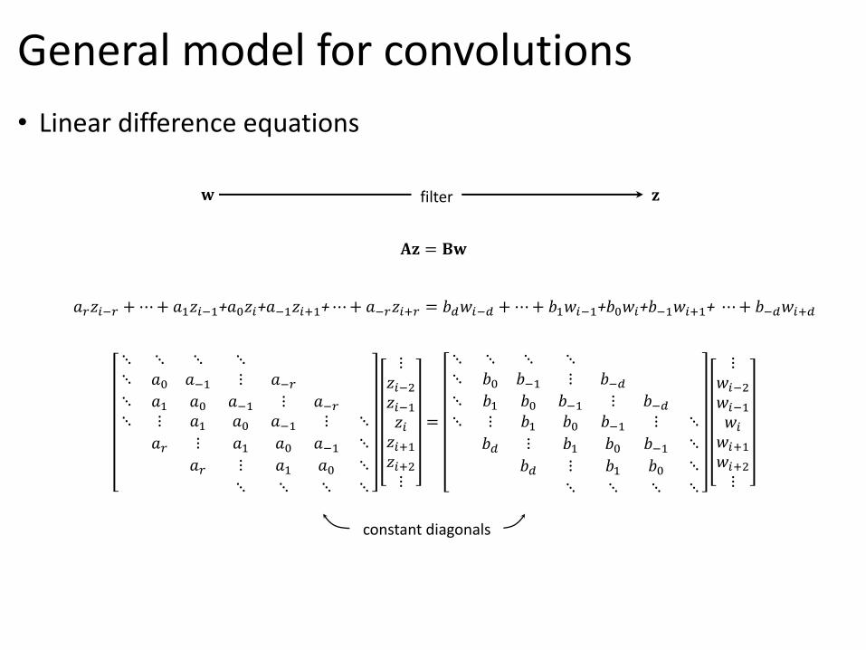
General model for convolutions
• Linear difference equations
𝐀𝐳 = 𝐁𝐰
⋱ ⋱ ⋱ ⋱⋱ 𝑎0 𝑎−1 ⋮ 𝑎−𝑟⋱ 𝑎1 𝑎0 𝑎−1 ⋮ 𝑎−𝑟⋱ ⋮ 𝑎1 𝑎0 𝑎−1 ⋮ ⋱
𝑎𝑟 ⋮ 𝑎1 𝑎0 𝑎−1 ⋱
𝑎𝑟 ⋮ 𝑎1 𝑎0 ⋱
⋱ ⋱ ⋱ ⋱
⋮𝑧𝑖−2𝑧𝑖−1𝑧𝑖𝑧𝑖+1𝑧𝑖+2⋮
=
⋱ ⋱ ⋱ ⋱⋱ 𝑏0 𝑏−1 ⋮ 𝑏−𝑑⋱ 𝑏1 𝑏0 𝑏−1 ⋮ 𝑏−𝑑⋱ ⋮ 𝑏1 𝑏0 𝑏−1 ⋮ ⋱
𝑏𝑑 ⋮ 𝑏1 𝑏0 𝑏−1 ⋱
𝑏𝑑 ⋮ 𝑏1 𝑏0 ⋱
⋱ ⋱ ⋱ ⋱
⋮𝑤𝑖−2
𝑤𝑖−1
𝑤𝑖
𝑤𝑖+1
𝑤𝑖+2
⋮
constant diagonals
𝑎𝑟𝑧𝑖−𝑟 +⋯+ 𝑎1𝑧𝑖−1+𝑎0𝑧𝑖+𝑎−1𝑧𝑖+1+⋯+ 𝑎−𝑟𝑧𝑖+𝑟 = 𝑏𝑑𝑤𝑖−𝑑 +⋯+ 𝑏1𝑤𝑖−1+𝑏0𝑤𝑖+𝑏−1𝑤𝑖+1+ ⋯+ 𝑏−𝑑𝑤𝑖+𝑑
filter 𝐳𝐰 𝐳𝐳

finite impulse response support (FIR)
⋮𝑥𝑖−2𝑥𝑖−1𝑥𝑖𝑥𝑖+1𝑥𝑖+2⋮
=
⋱ ⋱ ⋱ ⋱⋱ 𝑏0 𝑏−1 ⋮ 𝑏−𝑠⋱ 𝑏1 𝑏0 𝑏−1 ⋮ 𝑏−𝑠⋱ ⋮ 𝑏1 𝑏0 𝑏−1 ⋮ ⋱
𝑏𝑠 ⋮ 𝑏1 𝑏0 𝑏−1 ⋱
𝑏𝑠 ⋮ 𝑏1 𝑏0 ⋱
⋱ ⋱ ⋱ ⋱
⋮𝑤𝑖−2
𝑤𝑖−1
𝑤𝑖
𝑤𝑖+1
𝑤𝑖+2
⋮
• Decompose into direct and recursive parts
𝐱 𝐳recursive
𝑥𝑖 = 𝑏𝑠𝑤𝑖−𝑠 +⋯+ 𝑏1𝑤𝑖−1+𝑏0𝑤𝑖+𝑏−1𝑤𝑖+1+ ⋯+ 𝑏−𝑠𝑤𝑖+𝑠
direct part is what we think of as convolutionit is like a matrix multiplication 𝐱 = 𝐁𝐰
𝑂(𝑠 𝑛)
General model for convolutions
𝑎𝑟𝑧𝑖−𝑟 +⋯+ 𝑎1𝑧𝑖−1+𝑎0𝑧𝑖+𝑎−1𝑧𝑖+1+⋯+ 𝑎−𝑟𝑧𝑖+𝑟 = 𝑥𝑖
recursive part is the inverse of a convolutionit is like a linear system 𝐀𝐳 = 𝐱
infinite impulse response support (IIR)
⋱ ⋱ ⋱ ⋱⋱ 𝑎0 𝑎−1 ⋮ 𝑎−𝑟⋱ 𝑎1 𝑎0 𝑎−1 ⋮ 𝑎−𝑟⋱ ⋮ 𝑎1 𝑎0 𝑎−1 ⋮ ⋱
𝑎𝑟 ⋮ 𝑎1 𝑎0 𝑎−1 ⋱
𝑎𝑟 ⋮ 𝑎1 𝑎0 ⋱
⋱ ⋱ ⋱ ⋱
⋮𝑧𝑖−2𝑧𝑖−1𝑧𝑖𝑧𝑖+1𝑧𝑖+2⋮
=
⋮𝑥𝑖−2𝑥𝑖−1𝑥𝑖𝑥𝑖+1𝑥𝑖+2⋮
direct𝐰 filter 𝐳𝐰 𝐳𝐳direct𝐰 𝐳recursive
𝐀𝐳 = 𝐁𝐰𝐱 = 𝐁𝐰 𝐀𝐳 = 𝐱

𝐄𝐳 = √𝑎0
⋱ ⋱ ⋱ ⋱1 𝑒1 ⋮ 𝑒𝑟
1 𝑒1 ⋮ 𝑒𝑟1 𝑒1 ⋮ ⋱
1 𝑒1 ⋱
1 ⋱⋱
𝐳 = 𝐲
anticausal 𝐳
General model for convolutions
• Decompose recursive part into causal and anticausal passes
direct𝐰 𝐱 causal 𝐲 anticausal 𝐳
𝑦𝑖 =1
√𝑎0𝑥𝑖 − 𝑑1𝑦𝑖−1 −⋯− 𝑑𝑟𝑦𝑖−𝑟
causal part is forward-substitution 𝐃𝐲 = 𝐱
𝑂(𝑟 𝑛)𝑧𝑖 =
1
√𝑎0𝑦𝑖 − 𝑒1𝑧𝑖+1 −⋯− 𝑒𝑟𝑧𝑖+𝑟
anticausal is back-substitution 𝐄𝐳 = 𝐲
𝑂(𝑟 𝑛)
𝐱 causal
𝐃𝐲 = √𝑎0
⋱⋱ 1⋱ 𝑑1 1
⋱ ⋮ 𝑑1 1
𝑑𝑟 ⋮ 𝑑1 1
𝑑𝑟 ⋮ 𝑑1 1
⋱ ⋱ ⋱ ⋱
𝐲 = 𝐱
𝐳recursive𝐱
𝐀𝐳 = 𝐱𝐃𝐲 = 𝐱 𝐄𝐳 = 𝐲𝐱 = 𝐁𝐰

recursive filter
Downsampling with cardinal cubic B-splines
prefiltered
post-processed output
input
Catmull-Rom
t
cardinal cubic B-spline
tinfinite support
cubic B-spline
t
prefiltered
[Nehab & Hoppe 2014]
input
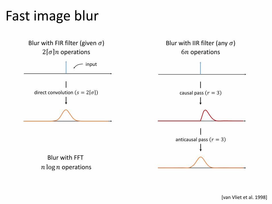
direct convolution 𝑠 = 2 𝜎
2 𝜎 𝑛 operations
Fast image blur
Blur with FIR filter (given 𝜎)
causal pass 𝑟 = 3
anticausal pass 𝑟 = 3
6𝑛 operations
Blur with IIR filter (any 𝜎)
Blur with FFT
𝑛 log𝑛 operations
[van Vliet et al. 1998]

??
What do near input boundaries?

Infinite input extensionsrepeat periodically
filter
reflect periodically
filter
constant padding
filter
periodic repetitionclamp to border
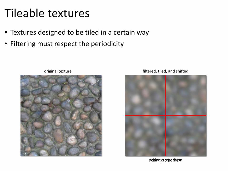
Tileable textures
• Textures designed to be tiled in a certain way
• Filtering must respect the periodicity
original texture filtered, tiled, and shifted

Dealing with boundaries in practice
• In the frequency domain• DFT/DCT imply infinite extensions
• Computations are exact even for IIR filters
• In the time domain• Direct convolution can decide out of bounds input arbitrarily
• Recursive filters must define out of bounds outputs!

even more wasted computation
filtered
even more wasted memory
padded
filtered
more wasted computation
padded
more wasted memorywasted memory
padded
wasted computation
filtered
Approximation by input padding
input
approximation
output
amount of padding dependson impulse response ”support”

Outline of talk
• Introduction• Recursive filters are very useful
• Initialization at the boundaries is an important problem
• Exact recursive filtering of infinite input extensions• Closed-form formulas available for the first time
• Enable simple and effective algorithms
• Parallelization• Fastest recursive filtering algorithms to date
• First to filter infinite extensions exactly

finite output
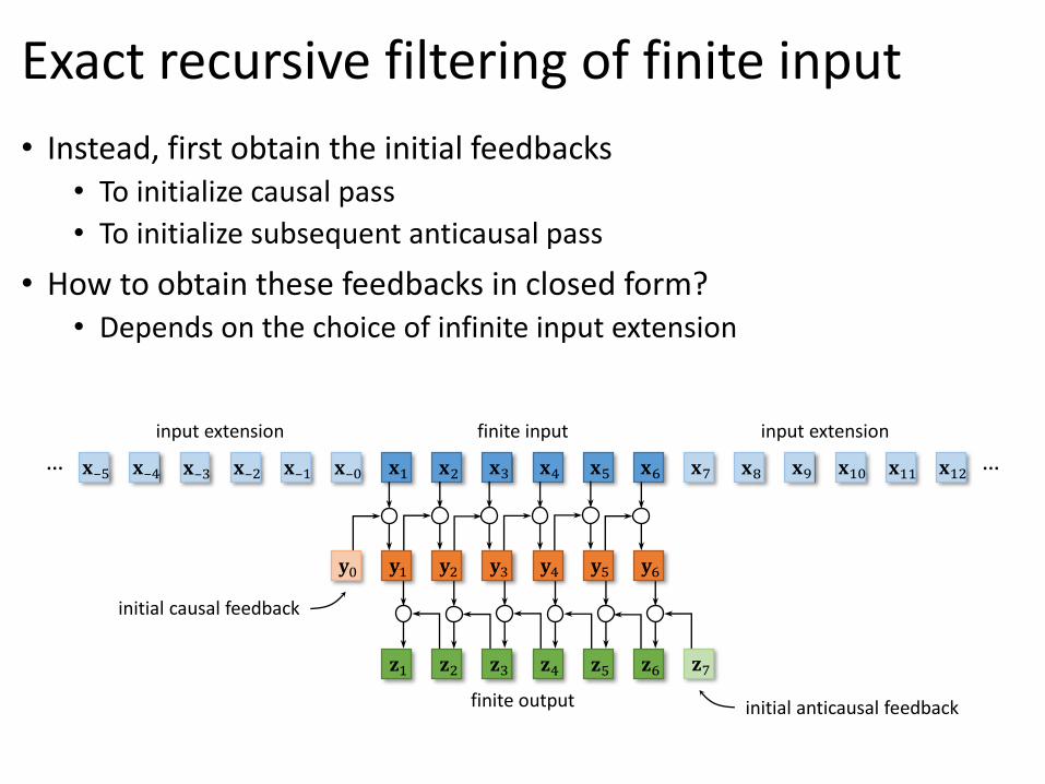
Exact recursive filtering of finite input
finite input
𝐱2 𝐱4 𝐱5 𝐱6𝐱1 𝐱3
input extension
𝐱–3 𝐱–1 𝐱–0𝐱–2𝐱–4𝐱–5… 𝐱8 𝐱10𝐱7 𝐱9 𝐱11 𝐱12 …input extension
𝐳8 𝐳10𝐳9 𝐳11 𝐳12 …𝐳5𝐳3𝐳2𝐳1 𝐳6𝐳4 𝐳7
𝐲2 𝐲4 𝐲5 𝐲6𝐲1 𝐲3 𝐲8 𝐲10𝐲7 𝐲9 𝐲11 𝐲12 …𝐲0… 𝐲–2 𝐲–1𝐲–3𝐲–4𝐲–5
finite output
Exact recursive filtering of finite input
• Instead, first obtain the initial feedbacks• To initialize causal pass
• To initialize subsequent anticausal pass
• How to obtain these feedbacks in closed form?• Depends on the choice of infinite input extension
initial causal feedback
initial anticausal feedback
finite inputinput extension
𝐱–3 𝐱–1 𝐱–0𝐱–2𝐱–4𝐱–5… 𝐱8 𝐱10𝐱7 𝐱9 𝐱11 𝐱12 …input extension
𝐳5𝐳3𝐳2𝐳1 𝐳6𝐳4 𝐳7
𝐱2 𝐱4 𝐱5 𝐱6𝐱1 𝐱3
𝐲2 𝐲4 𝐲5 𝐲6𝐲1 𝐲3𝐲0
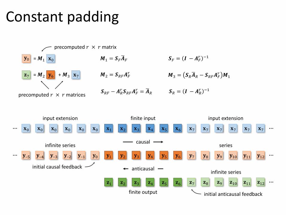
Constant padding
𝐲8 𝐲10𝐲7 𝐲9 𝐲11 𝐲12 …series
finite input
𝐱2 𝐱4 𝐱5 𝐱6𝐱1 𝐱3
input extension
𝐳5𝐳3𝐳2𝐳1 𝐳6𝐳4
anticausal
𝐲2 𝐲4 𝐲5 𝐲6𝐲1 𝐲3
causal
𝐱0 𝐱0 𝐱0𝐱0𝐱0𝐱0…
𝐲–2 𝐲–1𝐲–3𝐲–4𝐲–5…infinite series
𝐲0
𝐲0 = 𝑴1 𝐱0
initial causal feedback
𝐳8 𝐳10𝐳9 𝐳11 𝐳12 …infinite series
𝐳7
= 𝑴2𝐳7 + 𝑴3𝐲6 𝐱7
initial anticausal feedback
𝐱7 𝐱7𝐱7 𝐱7 𝐱7 𝐱7 …input extension
𝑴1 = 𝑺𝐹ഥ𝑨𝐹 𝑺𝐹 = 𝑰 − 𝑨𝐹𝑟 −1
𝑴2 = 𝑺𝑅𝐹𝑨𝐹𝑟
𝑺𝑅𝐹 − 𝑨𝑅𝑟𝑺𝑅𝐹𝑨𝐹
𝑟 = ഥ𝑨𝑅
𝑴3 = 𝑺𝑅ഥ𝑨𝑅 − 𝑺𝑅𝐹𝑨𝐹𝑟 𝑴1
𝑺𝑅 = 𝑰 − 𝑨𝑅𝑟 −1
finite output
precomputed 𝑟 × 𝑟 matrix
precomputed 𝑟 × 𝑟 matrices

ሶ𝐲2 ሶ𝐲4 ሶ𝐲5 ሶ𝐲6ሶ𝐲1 ሶ𝐲30
1st causal2nd causal
𝐲2 𝐲4 𝐲5 𝐲6𝐲1 𝐲3
2nd anticausal
𝐳5𝐳3𝐳2𝐳1 𝐳6𝐳4 ሶ𝐳5ሶ𝐳3ሶ𝐳2ሶ𝐳1 ሶ𝐳6ሶ𝐳4 0
1st anticausal
Periodic repetition
finite input
𝐱2 𝐱4 𝐱5 𝐱6𝐱1 𝐱3
= 𝑴5𝐳1 ሶ𝐳1
𝐳1
initial anticausal feedback
𝐲6 = 𝑴4 ሶ𝐲6
𝐲6
initial causal feedback
𝑴4 = 𝑰 − 𝑨𝐹𝑛 −1
𝑴5 = 𝑰 − 𝑨𝑅𝑛 −1
finite output
input extension
𝐱3 𝐱5 𝐱6𝐱4𝐱2𝐱1… 𝐱2 𝐱4𝐱1 𝐱3 𝐱5 𝐱6 …input extension

ሷ𝐳5ሷ𝐳3ሷ𝐳2ሷ𝐳1 ሷ𝐳6ሷ𝐳4 0
1st anticausal
ሶ𝐲2 ሶ𝐲4 ሶ𝐲5 ሶ𝐲6ሶ𝐲1 ሶ𝐲30
1st causal
𝐲2 𝐲4 𝐲5 𝐲6𝐲1 𝐲3
2nd causal
Periodic reflection
finite input
𝐱2 𝐱4 𝐱5 𝐱6𝐱1 𝐱3
ሶ𝐲6 𝐲12= 𝑴8 + 𝑴9
ሷ𝐳1ሶ𝐲6𝐲12 = 𝑴6 + 𝑴7 𝑴7 = 𝑰 − 𝑨𝐹2ℎ −1
𝑲 ഥ𝑨𝑅−1
𝑰 − 𝑨𝐹𝑟𝑨𝑅
𝑟
𝑴6 = 𝑰 − 𝑨𝐹2ℎ −1
𝑨𝐹ℎ −𝑲𝑨𝑅
ℎ ഥ𝑨𝐹−1𝑨𝐹𝑟 ഥ𝑨𝑅
𝑴8 = 𝑲− 𝑨𝑅𝑟 −𝟏ഥ𝑨𝑅
𝑴9 = 𝑲− 𝑨𝑅𝑟 −𝟏ഥ𝑨𝑅𝑨𝐹
ℎ
𝐲12
initial causal feedback
initial anticausal feedbackfinite output
𝐳5𝐳3𝐳2𝐳1 𝐳6𝐳4
2nd anticausal
input extension
… …input extension

Is this correct? Is this fast?
• All required 𝑟 × 𝑟 matrices 𝑴1to 𝑴9 exist and can be precomputed• Proofs in the paper assume only filter stability
• Exact filtering for all infinite extensions takes 𝑂(𝑟 𝑛)• May require twice as much computation
• Real advantage comes with parallelization• No additional cost

Outline of talk
• Introduction• Recursive filters are very useful
• Initialization at the boundaries is an important problem
• Exact recursive filtering of infinite input extensions• Closed-form formulas available for the first time
• Enable simple and effective algorithms
• Parallelization• Fastest recursive filtering algorithms to date
• First to filter infinite extensions exactly

GPU
• • • ThreadsThreadsSharedMemor
y
SharedMemor
y
Global Memory
Modern GPU
• Many multiprocessors each supporting many hardware threads• 10k threads is typical
• On-chip shared memory within each multiprocessor• 48k to be shared by threads local to multiprocessor
• Global memory with high throughput but high latency• High throughput but high latency
• Challenge is hide latency and keeping all cores busy
Multiprocessor Multiprocessor

𝐱13 𝐱15 𝐱16𝐱12 𝐱14𝐱1 𝐱3 𝐱4 𝐱5𝐱2
Independent rows then columns
input
𝐱7 𝐱9 𝐱10 𝐱11𝐱6 𝐱8
output
𝐲1 𝐲3 𝐲4 𝐲5𝐲2 𝐲13 𝐲15 𝐲16𝐲12 𝐲14𝐲7 𝐲9 𝐲10 𝐲11𝐲6 𝐲80
causal
𝐳1 𝐳2 𝐳3 𝐳4 𝐳13 𝐳15𝐳14 𝐳16𝐳8𝐳7𝐳6𝐳5 𝐳10 𝐳11𝐳9 𝐳12 0
anticausal
[Ruijters and Thevenaz 2010]
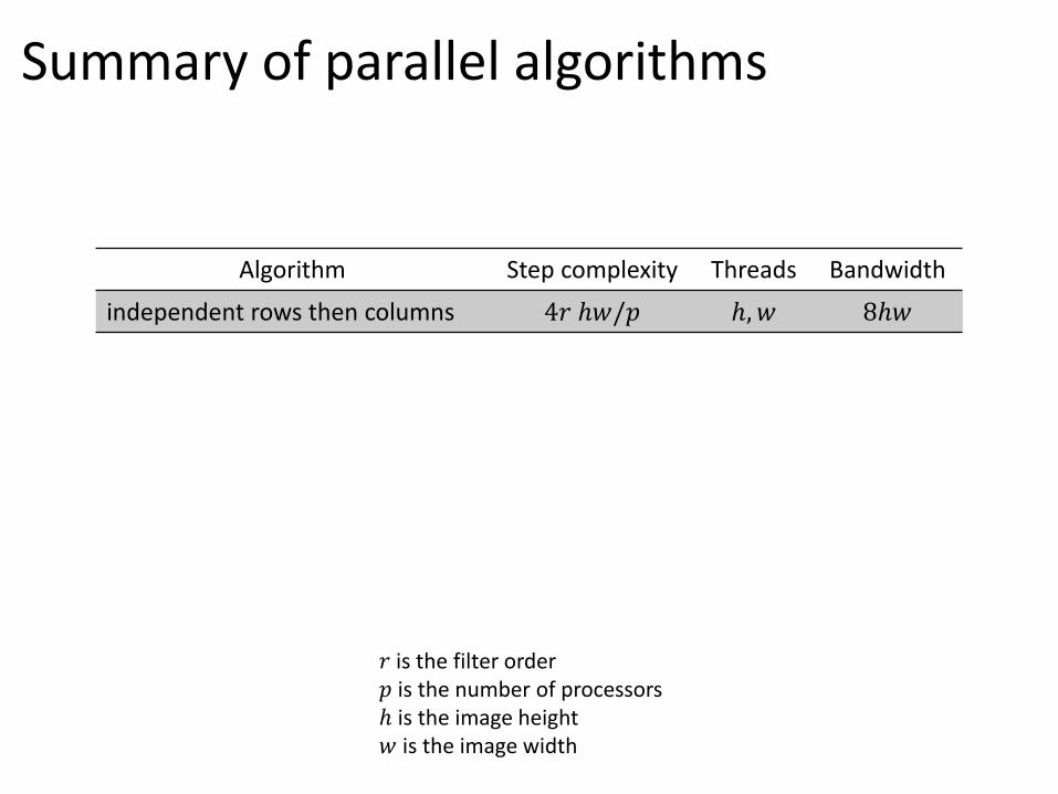
Summary of parallel algorithms
𝑟 is the filter order𝑝 is the number of processorsℎ is the image height𝑤 is the image width
Algorithm Step complexity Threads Bandwidth
independent rows then columns 4𝑟 ℎ𝑤/𝑝 ℎ, 𝑤 8ℎ𝑤

7
1
3
5
Thro
ughput
(GiP
/s)
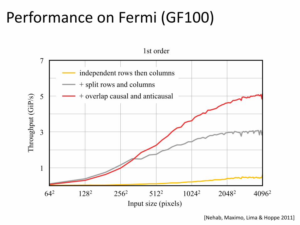
1st order
Input size (pixels)
642 1282 2562 5122 10242 20482 40962
[Nehab, Maximo, Lima & Hoppe 2011]
independent rows then columns
Performance on Fermi (GF100)

0 0 0 0
0 0 0 0
correct feedbacks
𝐳9𝐳1 𝐳5 𝐳13 0ሶ𝐳9ሶ𝐳1 ሶ𝐳5 ሶ𝐳13 0𝐳10 𝐳11𝐳9 𝐳12
2nd anticausal
𝐲13 𝐲15 𝐲16𝐲14
2nd causal
ሶ𝐲13 ሶ𝐲15 ሶ𝐲16ሶ𝐲14
1st causal
ሶ𝐲4 ሶ𝐲8 ሶ𝐲12 ሶ𝐲160 ሶ𝐲10 ሶ𝐲12ሶ𝐲9 ሶ𝐲11
1st causal
𝐲12𝐲9 𝐲10 𝐲11
2nd causal
ሶ𝐲5 ሶ𝐲7ሶ𝐲6 ሶ𝐲8
1st causal
𝐲4 𝐲16𝐲12𝐲8
correct feedbacks
0 𝐲5 𝐲7𝐲6 𝐲8
2nd causal1st causal
ሶ𝐲1 ሶ𝐲3 ሶ𝐲4ሶ𝐲2 𝐲3𝐲1 𝐲4𝐲2
2nd causal
𝐱13 𝐱15 𝐱16𝐱14𝐱1 𝐱3 𝐱4𝐱2 𝐱12𝐱9 𝐱10 𝐱11𝐱5 𝐱7𝐱6 𝐱8
ሶ𝐳1 ሶ𝐳2 ሶ𝐳3 ሶ𝐳4
1st anticausal
ሶ𝐳13 ሶ𝐳15ሶ𝐳14 ሶ𝐳16
1st anticausal
ሶ𝐳8ሶ𝐳7ሶ𝐳6ሶ𝐳5
1st anticausal
ሶ𝐳10 ሶ𝐳11ሶ𝐳9 ሶ𝐳12
1st anticausal
𝐳1 𝐳2 𝐳3 𝐳4
2nd anticausal
𝐳13 𝐳15𝐳14 𝐳16
2nd anticausal
𝐳8𝐳7𝐳6𝐳5
2nd anticausal
ሶ𝐳𝑏𝑖𝐳𝑏𝑖 𝐳𝑏(𝑖+1)= 𝑨𝑅𝑏 +
Split rows and columns into blocks
output
input
𝐱13 𝐱15 𝐱16𝐱14𝐱1 𝐱3 𝐱4𝐱2 𝐱12𝐱9 𝐱10 𝐱11𝐱5 𝐱7𝐱6 𝐱8
ሶ𝐲𝑏𝑖𝐲𝑏𝑖 𝐲𝑏(𝑖−1)= 𝑨𝐹𝑏 +
[Sung & Mitra 1986; Nehab, Maximo, Lima & Hoppe 2011]

Summary of parallel algorithms
𝑟 is the filter order𝑝 is the number of processorsℎ is the image height𝑤 is the image width
Algorithm Step complexity Threads Bandwidth
independent rows then columns 4𝑟 ℎ𝑤/𝑝 ℎ, 𝑤 8ℎ𝑤
+ split rows and columns ≈ 8𝑟 ℎ𝑤/𝑝 ℎ𝑤/𝑏 ≈ 9ℎ𝑤

7
1
3
5
Thro
ughput
(GiP
/s)
1st order
Input size (pixels)
642 1282 2562 5122 10242 20482 40962
[Nehab, Maximo, Lima & Hoppe 2011]
independent rows then columns
+ split rows and columns
Performance on Fermi (GF100)

correct feedbacks
𝐳9𝐳1 𝐳5 𝐳13 00 0 0 0ሷ𝐳10 ሷ𝐳11ሷ𝐳9 ሷ𝐳12
1st anticausal
𝐳10 𝐳11𝐳9 𝐳12
2nd anticausal
ሷ𝐳9ሷ𝐳1 ሷ𝐳5 ሷ𝐳13 0𝐳13 𝐳15𝐳14 𝐳16
2nd anticausal
ሷ𝐳13 ሷ𝐳15ሷ𝐳14 ሷ𝐳16
1st anticausal
0 0 0 0 𝐲15𝐲13 𝐲16𝐲14
2nd causal
𝐲12𝐲9 𝐲10 𝐲11
2nd causal
𝐲5 𝐲7𝐲6 𝐲8
2nd causal
𝐲3𝐲1 𝐲4𝐲2
2nd causal
ሶ𝐲12ሶ𝐲9 ሶ𝐲10 ሶ𝐲11
1st causal1st causal
ሶ𝐲1 ሶ𝐲3 ሶ𝐲4ሶ𝐲2 ሶ𝐲13 ሶ𝐲15 ሶ𝐲16ሶ𝐲14
1st causal
ሶ𝐲5 ሶ𝐲7ሶ𝐲6 ሶ𝐲8
1st causal
𝐲4 𝐲16𝐲12𝐲8
correct feedbacks
0
ሷ𝐳8ሷ𝐳7ሷ𝐳6ሷ𝐳5
1st anticausal
ሷ𝐳1 ሷ𝐳2 ሷ𝐳3 ሷ𝐳4
1st anticausal
𝐳8𝐳7𝐳6𝐳5
2nd anticausal
𝐳1 𝐳2 𝐳3 𝐳4
2nd anticausal
ሶ𝐲4 ሶ𝐲8 ሶ𝐲12 ሶ𝐲160
Overlap causal-anticausal processing
output
input
ሶ𝐲𝑏𝑖𝐲𝑏𝑖 𝐲𝑏(𝑖−1)= 𝑨𝐹𝑏 +
[Nehab, Maximo, Lima & Hoppe 2011]
ሷ𝐳𝑏𝑖𝐳𝑏𝑖 𝐳𝑏(𝑖+1)= 𝑨𝑅𝑏 + 𝐻 𝑨𝑅𝐵 𝑨𝐹𝑃 𝐲𝑏(𝑖−1) +
𝐱13 𝐱15 𝐱16𝐱14𝐱1 𝐱3 𝐱4𝐱2 𝐱12𝐱9 𝐱10 𝐱11𝐱5 𝐱7𝐱6 𝐱8

Summary of parallel algorithms
𝑟 is the filter order𝑝 is the number of processorsℎ is the image height𝑤 is the image width
Algorithm Step complexity Threads Bandwidth
independent rows then columns 4𝑟 ℎ𝑤/𝑝 ℎ, 𝑤 8ℎ𝑤
+ split rows and columns ≈ 8𝑟 ℎ𝑤/𝑝 ℎ𝑤/𝑏 ≈ 9ℎ𝑤
+ overlap causal with anticausal ≈ 8𝑟 ℎ𝑤/𝑝 ℎ𝑤/𝑏 ≈ 5ℎ𝑤
7
1
3
5
Thro
ughput
(GiP
/s)
1st order
Input size (pixels)
642 1282 2562 5122 10242 20482 40962
[Nehab, Maximo, Lima & Hoppe 2011]
independent rows then columns
+ split rows and columns
+ overlap causal and anticausal
Performance on Fermi (GF100)

Overlap causal, anticausal, rows, columns
[Nehab, Maximo, Lima & Hoppe 2011]

Stage 1
0
0
0
0
0
0
0
0
0
0
0
0
0
0
0
0
0
0
0 0 0 0 0 0 0 0 0
0 0 0 0 0 0 0 0 0
0
0
0
0
0
0
0
0
0
0
0
0
0
0
0
0
0
0
0 0 0 0 0 0 0 0 0
0 0 0 0 0 0 0 0 0
0 0 0 0 0 0 0 0 0
0 0 0 0 0 0 0 0 0
0
0
0
0
0
0
0
0
0
0
0
0
0
0
0
0
0
0
ഺ𝐮𝑚,𝑛𝐮𝑚,𝑛 𝐮𝑚,𝑛−1= 𝑨𝐹𝑏 𝑡
+ 𝑨𝑅𝐸 + 𝑨𝑅𝐵𝑨𝐹𝐵 𝑇 𝑨𝐹𝐵𝑡 +𝐳𝑚+1,𝑛 𝐲𝑚−1,𝑛𝑨𝑅
𝑏 𝑡+ 𝐳𝑚+1,𝑛𝐯𝑚,𝑛 𝐯𝑚,𝑛+1= + 𝑨𝑅𝐵𝑨𝐹𝑃𝑨𝑅𝐸𝐮𝑚,𝑛−1 𝐲𝑚−1,𝑛 𝐻 𝑨𝑅𝐵 𝑨𝐹𝐵
𝑡 + ሷሷ𝐯𝑚,𝑛𝐻 𝑨𝑅𝐵 𝑨𝐹𝑃𝑡 +
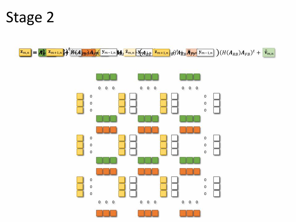
Stage 2
0
0
0
0
0
0
0
0
0
0
0
0
0
0
0
0
0
0
0 0 0 0 0 0 0 0 0
0 0 0 0 0 0 0 0 0
ሶ𝐲𝑚,𝑛𝐲𝑚,𝑛 𝐲𝑚−1,𝑛= 𝑨𝐹𝑏 + ሷ𝐳𝑚,𝑛𝐳𝑚,𝑛 𝐳𝑚+1,𝑛= 𝑨𝑅𝑏 + 𝐻 𝑨𝑅𝐵 𝑨𝐹𝑃 𝐲𝑚−1,𝑛 +

0
0
0
0
0
0
0
0
0
Stage 3
0
0
0
0
0
0
0
0
0
0 0 0 0 0 0 0 0 0
0 0 0 0 0 0 0 0 0

Stage 3
output

Summary of parallel algorithms
𝑟 is the filter order𝑝 is the number of processorsℎ is the image height𝑤 is the image width
Algorithm Step complexity Threads Bandwidth
independent rows then columns 4𝑟 ℎ𝑤/𝑝 ℎ, 𝑤 8ℎ𝑤
+ split rows and columns ≈ 8𝑟 ℎ𝑤/𝑝 ℎ𝑤/𝑏 ≈ 9ℎ𝑤
+ overlap causal with anticausal ≈ 8𝑟 ℎ𝑤/𝑝 ℎ𝑤/𝑏 ≈ 5ℎ𝑤
+ overlap rows with columns ≈ 8𝑟 ℎ𝑤/𝑝 ℎ𝑤/𝑏 ≈ 3ℎ𝑤

7
1
3
5
Thro
ughput
(GiP
/s)
1st order
Input size (pixels)
642 1282 2562 5122 10242 20482 40962
[Nehab, Maximo, Lima & Hoppe 2011]
+ overlap rows and columns
independent rows then columns
+ split rows and columns
+ overlap causal and anticausal
Performance on Fermi (GF100)

+ overlap rows and columns
[Nehab, Maximo, Lima & Hoppe 2011]
Input size (pixels)
642 1282 2562 5122 10242 20482 40962
2nd order
5
1
2
3
Thro
ughput
(GiP
/s)
4
overlap causal and anticausal
Performance on Fermi (GF100)

ഺ𝐮𝑚,𝑛𝐮𝑚,𝑛 𝐮𝑚,𝑛−1= 𝑨𝐹𝑏 𝑡
+ 𝑨𝑅𝐸 + 𝑨𝑅𝐵𝑨𝐹𝐵 𝑇 𝑨𝐹𝐵𝑡 +𝐳𝑚+1,𝑛 𝐲𝑚−1,𝑛
𝐲𝑚−1,𝑛𝑨𝑅𝑏 𝑡
+ 𝐳𝑚+1,𝑛𝐯𝑚,𝑛 𝐯𝑚,𝑛+1= + 𝑨𝑅𝐵𝑨𝐹𝑃𝑨𝑅𝐸𝐮𝑚,𝑛−1 𝐻 𝑨𝑅𝐵 𝑨𝐹𝐵𝑡 + ሷሷ𝐯𝑚,𝑛𝐻 𝑨𝑅𝐵 𝑨𝐹𝑃
𝑡 +𝑨𝑅𝑏 𝑡
+𝐯𝑚,𝑛 𝐯𝑚,𝑛+1= 𝐮𝑚,𝑛−1 𝐻 𝑨𝑅𝐵 𝑨𝐹𝑃𝑡 + ത𝐯𝑚,𝑛
𝐮𝑚,𝑛 𝐮𝑚,𝑛−1= 𝑨𝐹𝑏 𝑡
+ ഥ𝐮𝑚,𝑛
New trick for better performance
ሶ𝐲𝑚,𝑛𝐲𝑚,𝑛 𝐲𝑚−1,𝑛= 𝑨𝐹𝑏 +
ሷ𝐳𝑚,𝑛𝐳𝑚,𝑛 𝐳𝑚+1,𝑛= 𝑨𝑅𝑏 + 𝐻 𝑨𝑅𝐵 𝑨𝐹𝑃 𝐲𝑚−1,𝑛 +
sequentially find per-block column feedbacks
sequentially find per-block row feedbacks
ഥ𝐮𝑚,𝑛 ഺ𝐮𝑚,𝑛= 𝑨𝑅𝐸 + 𝑨𝑅𝐵𝑨𝐹𝐵 𝑇 𝑨𝐹𝐵𝑡 +𝐳𝑚+1,𝑛 𝐲𝑚−1,𝑛
ത𝐯𝑚,𝑛 𝐳𝑚+1,𝑛= + 𝑨𝑅𝐵𝑨𝐹𝑃𝑨𝑅𝐸𝐲𝑚−1,𝑛 𝐻 𝑨𝑅𝐵 𝑨𝐹𝐵
𝑡 + ሷሷ𝐯𝑚,𝑛
new fully parallel intermediate stage
(exactly the same as column processing)

Summary of parallel algorithms
Algorithm Step complexity Threads Bandwidth
independent rows then columns 4𝑟 ℎ𝑤/𝑝 ℎ, 𝑤 8ℎ𝑤
+ split rows and columns ≈ 8𝑟 ℎ𝑤/𝑝 ℎ𝑤/𝑏 ≈ 9ℎ𝑤
+ overlap causal with anticausal ≈ 8𝑟 ℎ𝑤/𝑝 ℎ𝑤/𝑏 ≈ 5ℎ𝑤
+ overlap rows with columns ≈ 8𝑟 ℎ𝑤/𝑝 ℎ𝑤/𝑏 ≈ 3ℎ𝑤
+ new trick ≈ 8𝑟 ℎ𝑤/𝑝 ℎ𝑤/𝑏 ≈ 3ℎ𝑤
𝑟 is the filter order𝑝 is the number of processorsℎ is the image height𝑤 is the image width

13
1
3
5
7
9
11
642 819221282 2562 5122 10242 20482 40962
Input size (pixels)
Thro
ughput
(GiP
/s)
overlap causal and anticausal
+ overlap rows and columns
+ new trick
Performance on Kepler (GK110)
3rd order4th order

642 819221282 2562 5122 10242 20482 40962
17
1
3
15
13
11
9
7
5
Input size (pixels)
Thro
ughput
(GiP
/s)
Performance on Pascal (GP102)
overlap causal and anticausal
+ overlap rows and columns
+ new trick
5th order

ሶ𝐲2 ሶ𝐲4 ሶ𝐲5 ሶ𝐲6ሶ𝐲1 ሶ𝐲30
1st causal
ሷ𝐳5ሷ𝐳3ሷ𝐳2ሷ𝐳1 ሷ𝐳6ሷ𝐳4 0
1st anticausal
𝐳5𝐳3𝐳2𝐳1 𝐳6𝐳4
2nd anticausal
𝐲2 𝐲4 𝐲5 𝐲6𝐲1 𝐲3
2nd causal
Back to infinite extensions
entire finite input
𝐱2 𝐱4 𝐱5 𝐱6𝐱1 𝐱3
ሶ𝐲6 𝐲12= 𝑴8 + 𝑴9
ሷ𝐳1ሶ𝐲6𝐲12 = 𝑴6 + 𝑴7 𝑴7 = 𝑰 − 𝑨𝐹2ℎ −1
𝑲 ഥ𝑨𝑅−1
𝑰 − 𝑨𝐹𝑟𝑨𝑅
𝑟
𝑴6 = 𝑰 − 𝑨𝐹2ℎ −1
𝑨𝐹ℎ −𝑲𝑨𝑅
ℎ ഥ𝑨𝐹−1𝑨𝐹𝑟 ഥ𝑨𝑅
𝑴8 = 𝑲− 𝑨𝑅𝑟 −𝟏ഥ𝑨𝑅
𝑴9 = 𝑲− 𝑨𝑅𝑟 −𝟏ഥ𝑨𝑅𝑨𝐹
ℎ
𝐲12
initial causal feedback
initial anticausal feedbackentire finite output
input extension
… …input extension
ሶ𝐲6
ሷ𝐳1

0
0
0
0
0
0
0
0
0
0
0
0
0
0
0
0
0
0
0 0 0 0 0 0 0 0 0
0 0 0 0 0 0 0 0 0
Back to infinite extensions
• Side effect of 2nd stage of parallel algorithm
• Just what we need to compute exact initial feedbacks!

13
1
3
5
7
9
11
642 819221282 2562 5122 10242 20482 40962
Input size (pixels)
Thro
ughput
(GiP
/s)
1st order (cubic B-spline interpolation)
[Chaurasia et al. 2015]
[Nehab et al. 2011]
padding
exact reflect
exact repeat
exact clamp to border
Performance on Kepler (GK110)

conv
cuFFT
[Chaurasia et al. 2015]
[Nehab et al. 2011]
642 819221282 2562 5122 10242 20482 40962
7
1
3
5
Input size (pixels)
Thro
ughput
(GiP
/s)
3rd order (2D Gaussian blur with 𝜎 = 𝑛/6)
Performance on Kepler (GK110)
padding
exact reflect
exact repeat
exact clamp to border

Summary
• Introduction• Recursive filters are very useful
• Initialization at the boundaries is an important problem
• Exact recursive filtering of infinite input extensions• Closed-form formulas available for the first time
• Enable simple and effective algorithms
• Parallelization• Fastest recursive filtering algorithms to date
• First to filter infinite extensions exactly

Thank you!
• Please download and use our code
https://github.com/andmax/gpufilter
• Questions?