Parallel MDOM for Rendering Participating Media

Ajit Hakke Patil – Daniele BernabeiCharly Collin – Ke Chen – Sumanta Pattanaik

Fabio Ganovelli

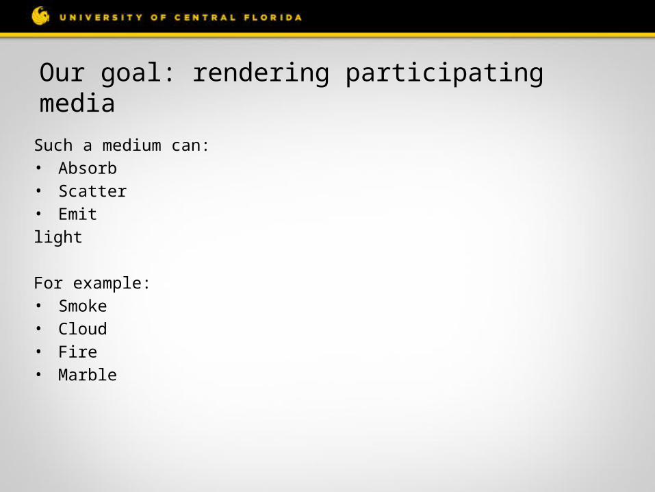
Our goal: rendering participating media

Such a medium can:• Absorb• Scatter• Emitlight

For example:• Smoke• Cloud• Fire• Marble

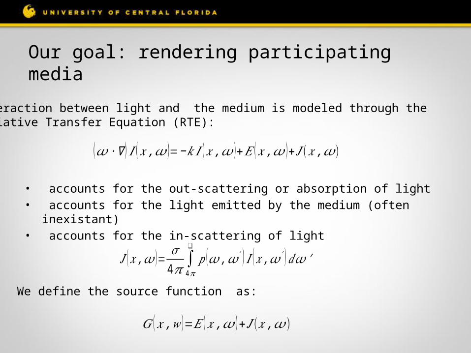
Our goal: rendering participating media

Interaction between light and the medium is modeled through theRadiative Transfer Equation (RTE):

(𝜔 ∙∇ ) 𝐼 (𝑥 ,𝜔 )=−𝑘𝐼 (𝑥 ,𝜔 )+𝐸 (𝑥 ,𝜔 )+ 𝐽 (𝑥 ,𝜔)

• accounts for the out-scattering or absorption of light• accounts for the light emitted by the medium (often inexistant)• accounts for the in-scattering of light

𝐽 (𝑥 ,𝜔 )= 𝜎4𝜋 ∫

4 𝜋

❑

𝑝 (𝜔 ,𝜔′ ) 𝐼 (𝑥 ,𝜔 ′) 𝑑𝜔 ′

We define the source function as:

𝐺 (𝑥 ,𝑤 )=𝐸 (𝑥 ,𝜔 )+ 𝐽 (𝑥 ,𝜔)

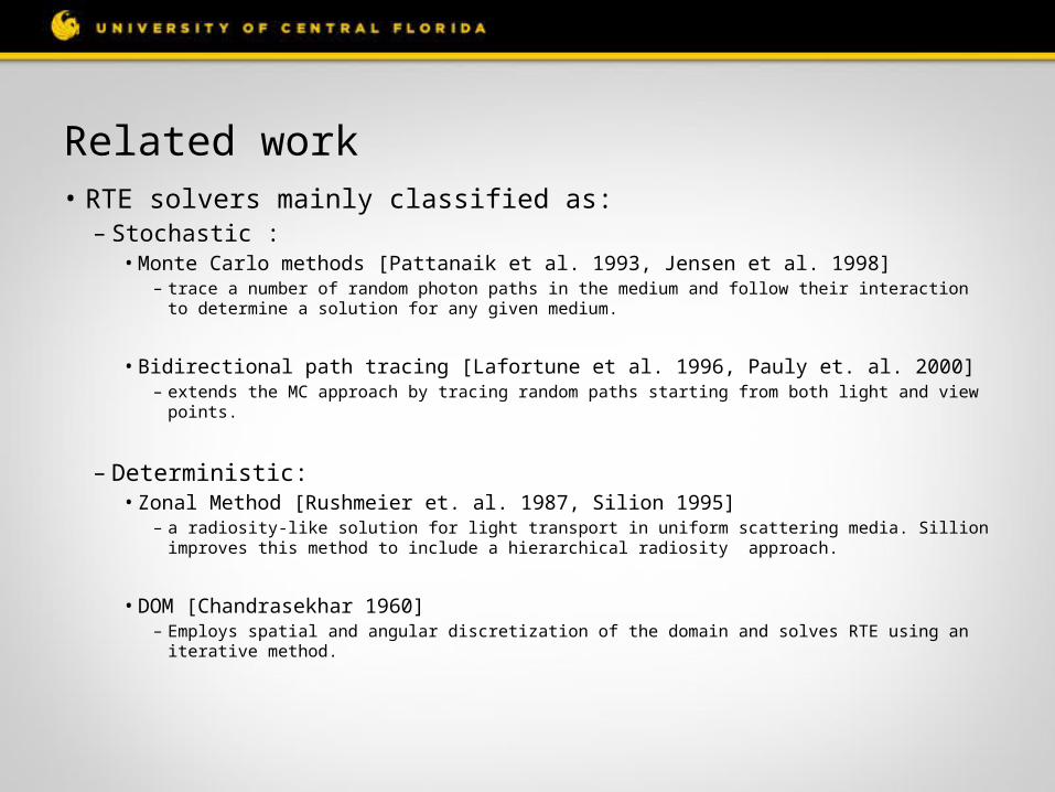
Related work• RTE solvers mainly classified as:

– Stochastic : • Monte Carlo methods [Pattanaik et al. 1993, Jensen et al. 1998]

– trace a number of random photon paths in the medium and follow their interaction to determine a solution for any given medium.

• Bidirectional path tracing [Lafortune et al. 1996, Pauly et. al. 2000]– extends the MC approach by tracing random paths starting from both light and view points.

– Deterministic:• Zonal Method [Rushmeier et. al. 1987, Silion 1995]

– a radiosity-like solution for light transport in uniform scattering media. Sillion improves this method to include a hierarchical radiosity approach.

• DOM [Chandrasekhar 1960]– Employs spatial and angular discretization of the domain and solves RTE using an iterative

method.

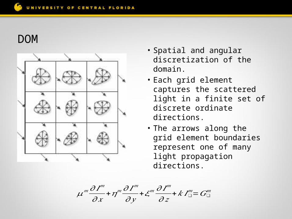
DOM• Spatial and angular

discretization of the domain.• Each grid element captures

the scattered light in a finite set of discrete ordinate directions.

• The arrows along the grid element boundaries represent one of many light propagation directions.

𝜇𝑚 𝜕 𝐼𝑚

𝜕𝑥+𝜂𝑚 𝜕 𝐼𝑚

𝜕 𝑦+𝜉𝑚 𝜕 𝐼𝑚

𝜕 𝑧+𝑘 𝐼❑

𝑚=𝐺❑𝑚

Related work• DOM grid schemes are classified based on their treatment of the linear

streaming operator () – Characteristic schemes

• Short characteristic schemes• Long characteristic schemes

– Finite Element– Integro-Interpolational schemes

• DOM limitations:– Ray effects : related to the angular discretization scheme.– False scattering or numerical smearing: related to the spatial

discretization.

Related work

• Other GPU based volumetric scattering methods:– Diffusion approximation based:

• Lattice Boltzmann solution. [Bernabei et. al]• Works well for homogeneous media.

– DOM based approaches:• GPU port of Fattal’s LPM method [Gruson et. al]• Cannot handle directional light sources as it is based on

regular DOM.

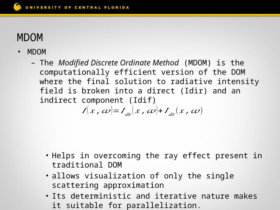
MDOM• MDOM

– The Modified Discrete Ordinate Method (MDOM) is the computationally efficient version of the DOM where the final solution to radiative intensity field is broken into a direct (Idir) and an indirect component (Idif)

• Helps in overcoming the ray effect present in traditional DOM• allows visualization of only the single scattering approximation• Its deterministic and iterative nature makes it suitable for

parallelization.

𝐼 (𝑥 ,𝜔 )=𝐼𝑑𝑖𝑟 (𝑥 ,𝜔 )+𝐼𝑑𝑖𝑟 (𝑥 ,𝜔)

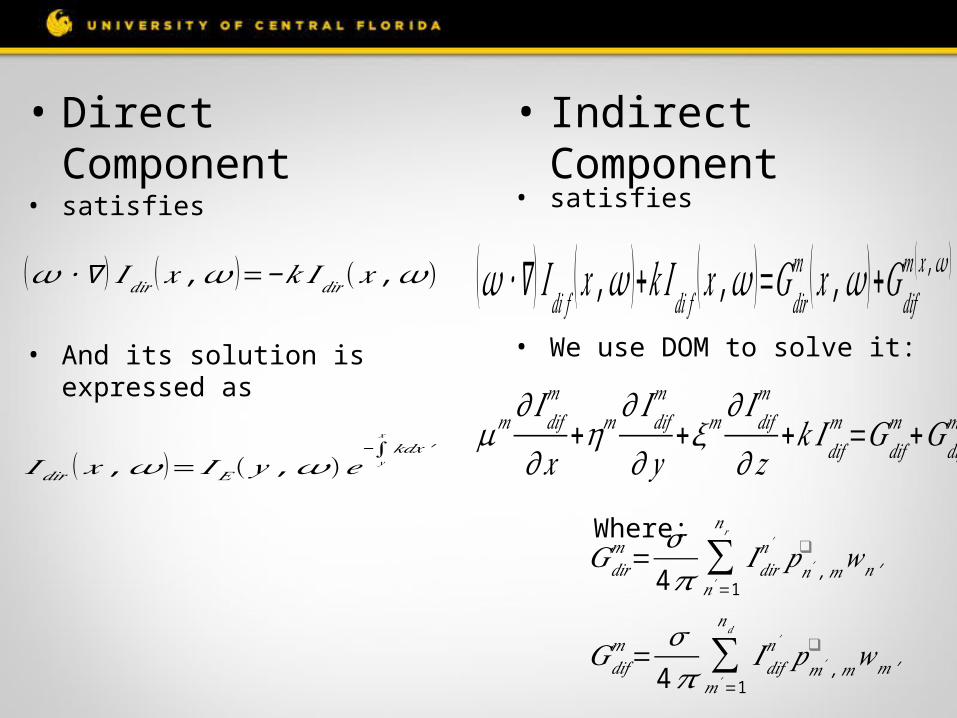
• satisfies

• And its solution is expressed as

(𝜔 ∙∇ ) 𝐼𝑑𝑖𝑟 (𝑥 ,𝜔 )=−𝑘𝐼𝑑𝑖𝑟 (𝑥 ,𝜔)

• Direct Component

• satisfies

• We use DOM to solve it:

Where:

• Indirect Component

𝐼𝑑𝑖𝑟 ( 𝑥 ,𝜔 )=𝐼𝐸(𝑦 ,𝜔)𝑒−∫

𝑦

𝑥

𝑘𝑑𝑥 ′

(𝜔 ∙∇ ) 𝐼𝑑𝑖 𝑓 (𝑥 ,𝜔 )+𝑘 𝐼𝑑𝑖 𝑓 ( 𝑥 ,𝜔 )=𝐺𝑑𝑖𝑟𝑚 (𝑥 ,𝜔 )+𝐺𝑑𝑖𝑓

𝑚 (𝑥 ,𝜔 )

𝜇𝑚 𝜕 𝐼𝑑𝑖𝑓𝑚

𝜕 𝑥+𝜂𝑚 𝜕 𝐼𝑑𝑖𝑓

𝑚

𝜕 𝑦+𝜉𝑚 𝜕 𝐼𝑑𝑖𝑓

𝑚

𝜕 𝑧+𝑘𝐼𝑑𝑖𝑓

𝑚 =𝐺𝑑𝑖𝑓𝑚 +𝐺𝑑𝑖𝑓

𝑚

𝐺𝑑𝑖𝑟𝑚 = 𝜎

4 𝜋 ∑𝑛 ′=1

𝑛𝑟

𝐼𝑑𝑖𝑟𝑛′ 𝑝

𝑛′ ,𝑚

❑ 𝑤𝑛 ′

𝐺𝑑𝑖𝑓𝑚 = 𝜎

4 𝜋 ∑𝑚 ′=1

𝑛𝑑

𝐼𝑑𝑖𝑓𝑛′ 𝑝

𝑚′ ,𝑚

❑ 𝑤𝑚 ′

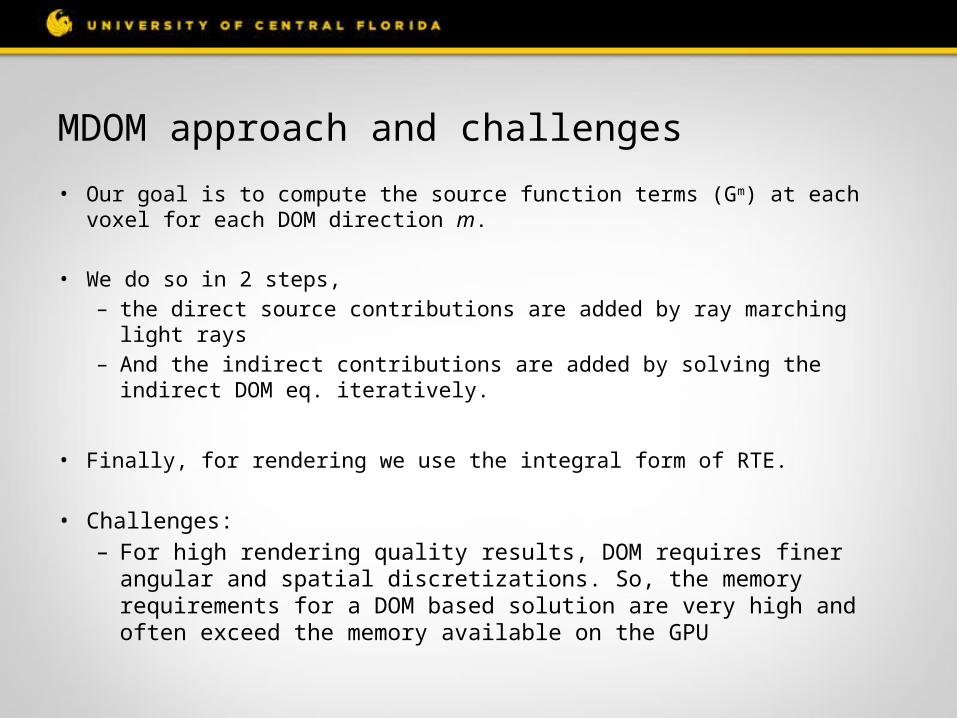
MDOM approach and challenges

• Our goal is to compute the source function terms (Gm) at each voxel for each DOM direction m.

• We do so in 2 steps, – the direct source contributions are added by ray marching light rays – And the indirect contributions are added by solving the indirect DOM eq.

iteratively.

• Finally, for rendering we use the integral form of RTE.

• Challenges:– For high rendering quality results, DOM requires finer angular and spatial

discretizations. So, the memory requirements for a DOM based solution are very high and often exceed the memory available on the GPU

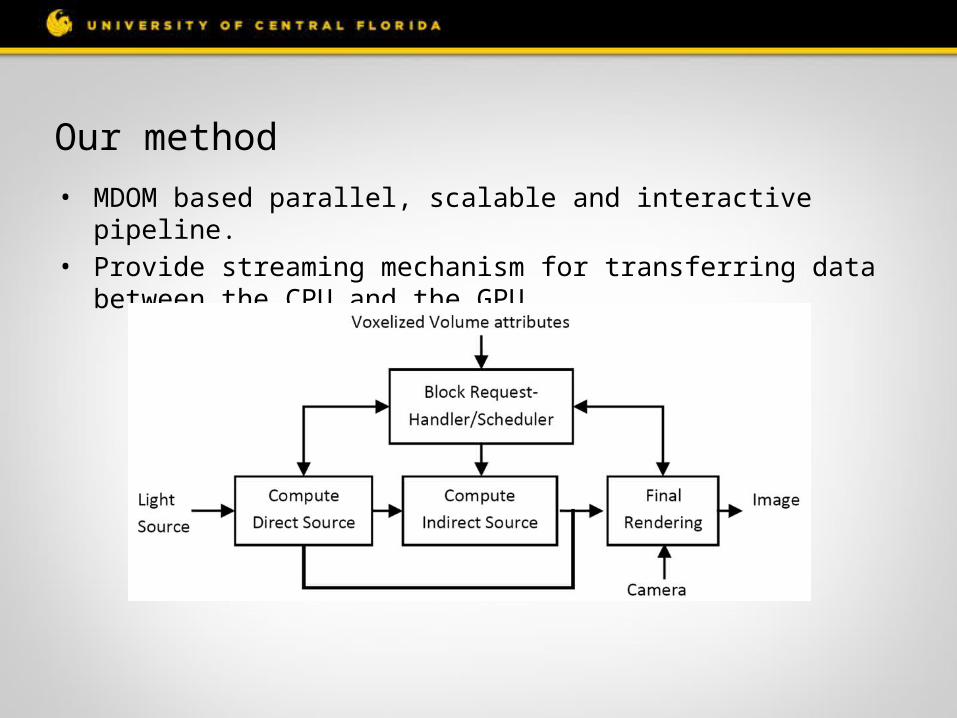
Our method

• MDOM based parallel, scalable and interactive pipeline.• Provide streaming mechanism for transferring data between the CPU and

the GPU

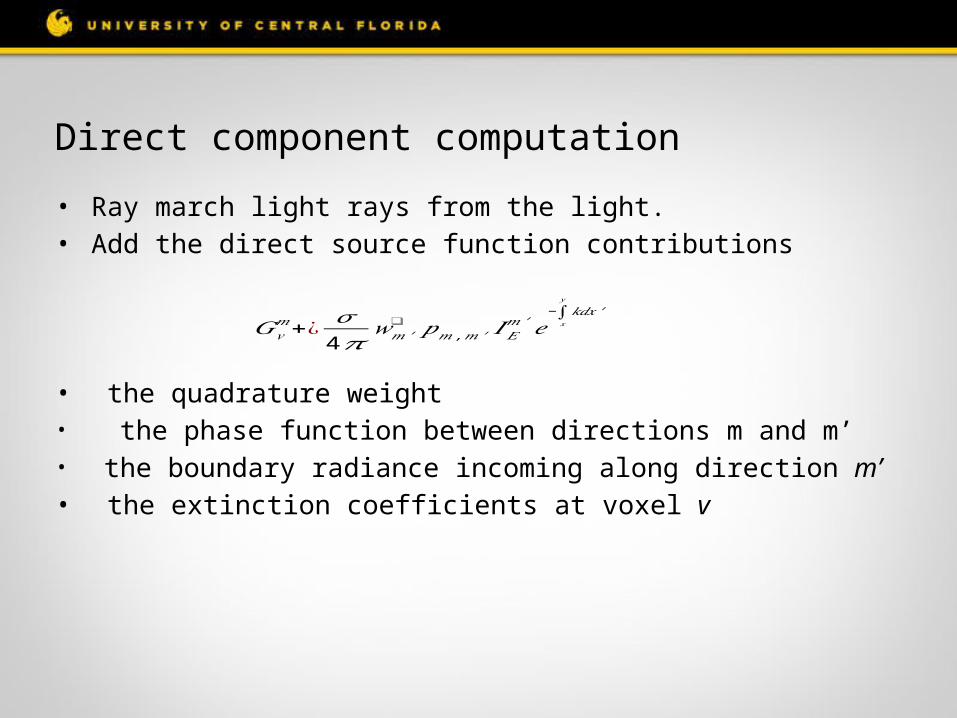
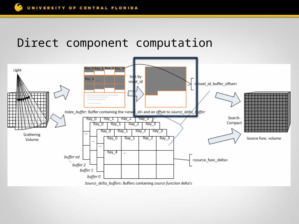
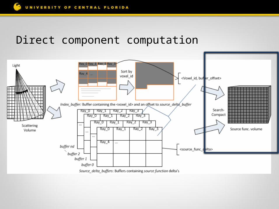
Direct component computation

• Ray march light rays from the light.• Add the direct source function contributions

• the quadrature weight• the phase function between directions m and m’• the boundary radiance incoming along direction m’ • the extinction coefficients at voxel v

𝐺𝑣𝑚+¿ 𝜎

4𝜋𝑤𝑚 ′

❑ 𝑝𝑚 ,𝑚 ′ 𝐼𝐸𝑚 ′ 𝑒

−∫𝑥

𝑦

𝑘𝑑𝑥 ′

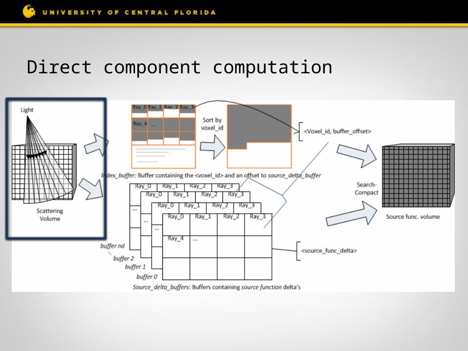
Direct component computation

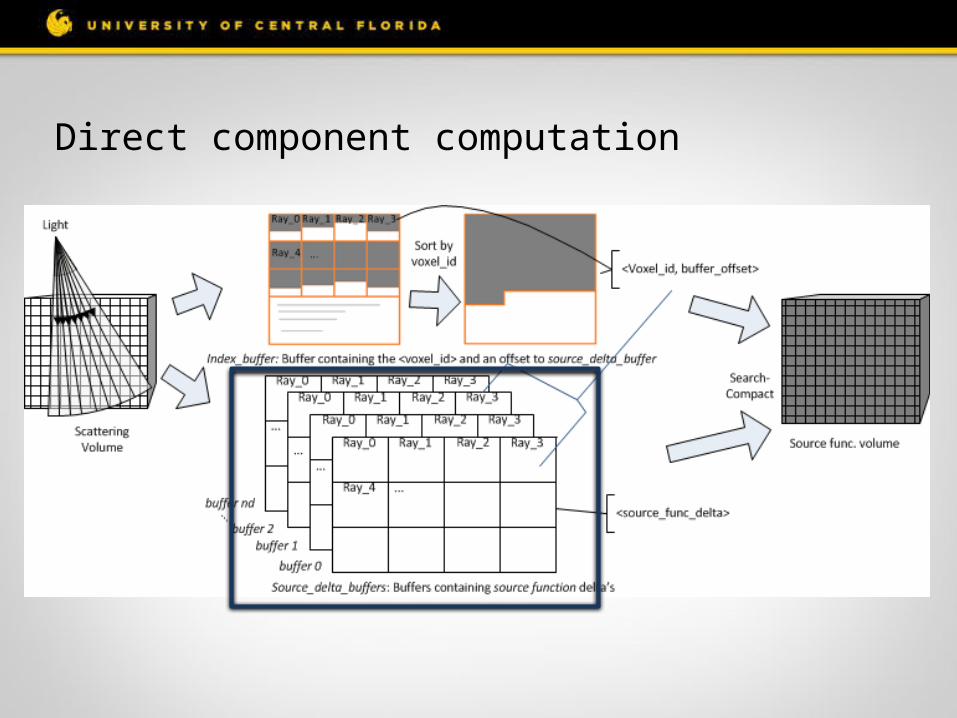
Direct component computation

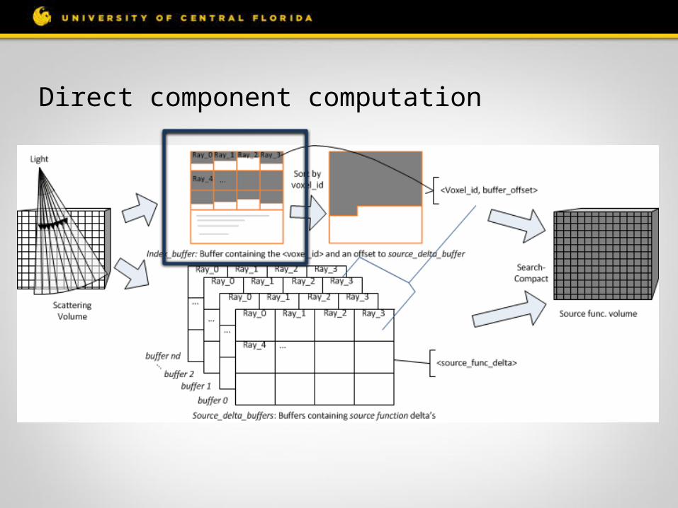
Direct component computation

Direct component computation

Direct component computation

Direct component computation

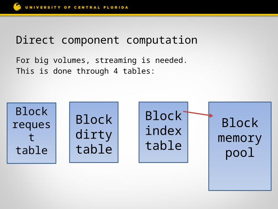
For big volumes, streaming is needed.This is done through 4 tables:

Block request

table

Block dirty table

Block indextable

Block memory

pool

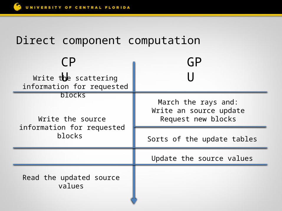
Direct component computation

GPUCPUWrite the scattering information for

requested blocks

March the rays and:Write an source update

Request new blocks

Sorts of the update tables

Write the source information for requested blocks

Update the source values

Read the updated source values

Indirect component computation

• Iterative solution to the DOM eq. for the diffuse/indirect component, where each iteration corresponds to an scattering event.

• During each iteration the scattering contributions from the last scattering iteration () are used as the source function for the current iteration.

• We iterate the indirect component computation until convergence:

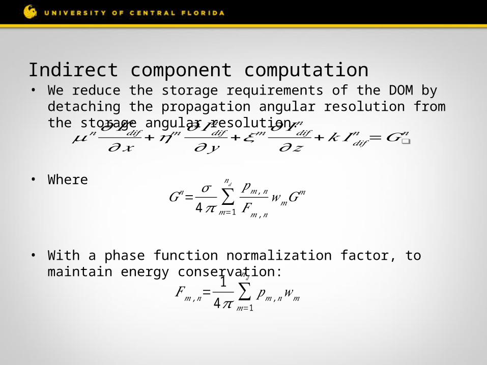
Indirect component computation• We reduce the storage requirements of the DOM by detaching the

propagation angular resolution from the storage angular resolution.

• Where

• With a phase function normalization factor, to maintain energy conservation:

𝜇𝑛 𝜕 𝐼𝑑𝑖𝑓𝑛

𝜕𝑥+𝜂𝑚 𝜕 𝐼𝑑𝑖𝑓

𝑛

𝜕 𝑦+𝜉𝑚 𝜕 𝐼𝑑𝑖𝑓

𝑛

𝜕 𝑧+𝑘 𝐼𝑑𝑖𝑓

𝑛 =𝐺❑𝑛

𝐺𝑛= 𝜎4𝜋 ∑

𝑚=1

𝑛𝑑 𝑝𝑚 ,𝑛

𝐹𝑚 ,𝑛

𝑤𝑚 𝐺𝑚

𝐹𝑚 ,𝑛=14𝜋 ∑

𝑚=1

𝑛𝑑

𝑝𝑚 ,𝑛𝑤𝑚

Indirect component computation

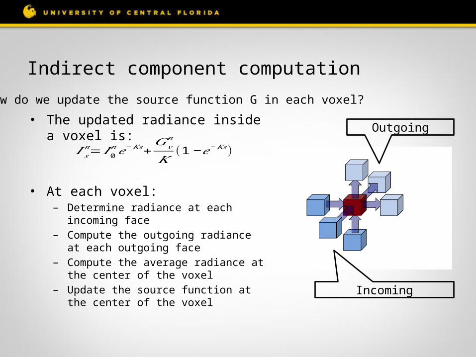
How do we update the source function G in each voxel?

Incoming

Outgoing• The updated radiance inside a voxel is:

• At each voxel:– Determine radiance at each incoming face– Compute the outgoing radiance at each

outgoing face– Compute the average radiance at the center of

the voxel– Update the source function at the center of

the voxel

𝐼 𝑠𝑛= 𝐼0

𝑛𝑒−𝐾𝑠+𝐺𝑣

𝑛

𝐾(1−𝑒−𝐾𝑠)

Indirect component computation

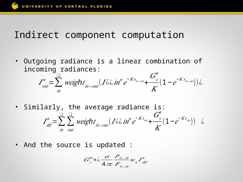
• Outgoing radiance is a linear combination of incoming radiances:

• Similarly, the average radiance is:

• And the source is updated :

𝐼𝑜𝑢𝑡𝑛 =∑

𝑖𝑛

❑

h𝑤𝑒𝑖𝑔 𝑡𝑖𝑛→𝑜𝑢𝑡( 𝐼¿¿ 𝑖𝑛𝑛𝑒−𝐾 𝑠𝑖𝑛→ 𝑜𝑢𝑡+𝐺𝑣

𝑛

𝐾(1−𝑒−𝐾 𝑠𝑖𝑛→𝑜𝑢𝑡))¿

𝐼𝑑𝑖𝑓𝑛 =∑

𝑖𝑛

❑

∑𝑜𝑢𝑡

❑

h𝑤𝑒𝑖𝑔 𝑡 𝑖𝑛→𝑜𝑢𝑡(𝐼 ¿¿ 𝑖𝑛𝑛𝑒−𝐾 𝑠𝑎𝑣𝑔+𝐺𝑣

𝑛

𝐾(1−𝑒−𝐾 𝑠𝑎𝑣𝑔))  ¿

𝐺𝑣𝑚+¿ 𝜎

4𝜋𝑝𝑛 ,𝑚

𝐹𝑛 ,𝑚

𝑤𝑛 𝐼𝑑𝑖𝑓𝑛

Indirect component computation

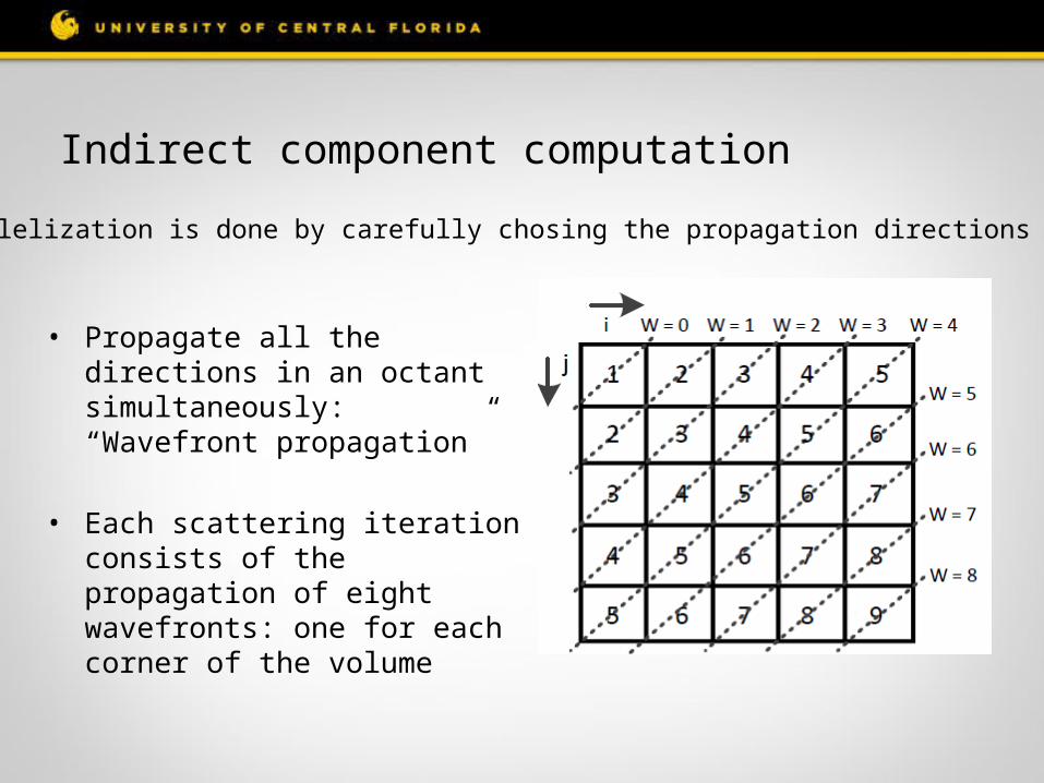
Parallelization is done by carefully chosing the propagation directions

• Propagate all the directions in an octant simultaneously: “Wavefront propagation”

• Each scattering iteration consists of the propagation of eight wavefronts: one for each corner of the volume

Indirect component computation

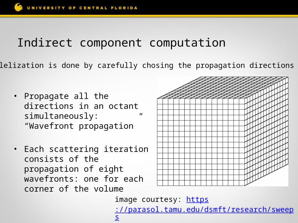
Parallelization is done by carefully chosing the propagation directions

• Propagate all the directions in an octant simultaneously: “Wavefront propagation”

• Each scattering iteration consists of the propagation of eight wavefronts: one for each corner of the volume

image courtesy: https://parasol.tamu.edu/dsmft/research/sweeps/

Indirect component computation

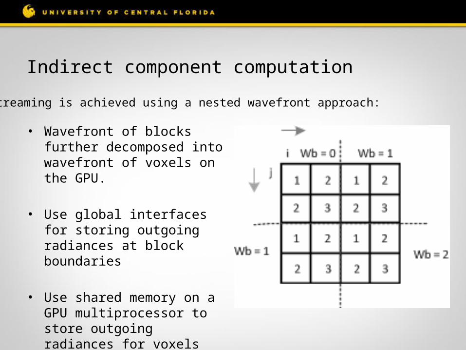
Streaming is achieved using a nested wavefront approach:

• Wavefront of blocks further decomposed into wavefront of voxels on the GPU.

• Use global interfaces for storing outgoing radiances at block boundaries

• Use shared memory on a GPU multiprocessor to store outgoing radiances for voxels not on block boundary

Visualization

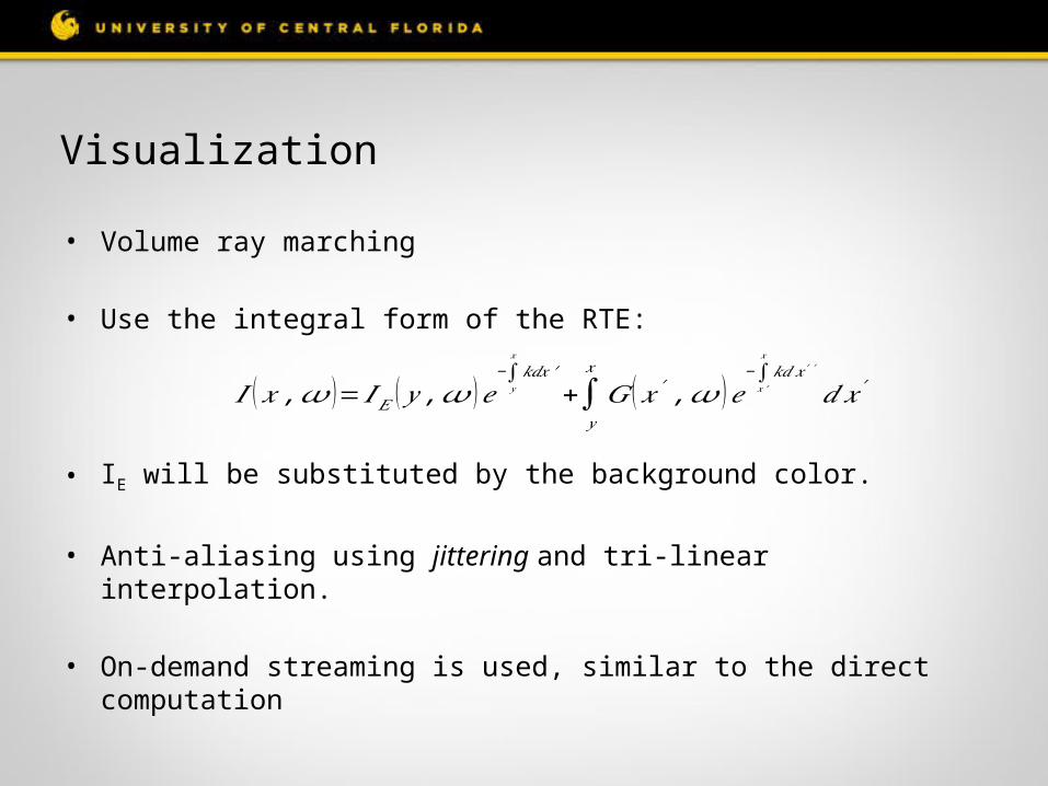
• Volume ray marching

• Use the integral form of the RTE:

• IE will be substituted by the background color.

• Anti-aliasing using jittering and tri-linear interpolation.

• On-demand streaming is used, similar to the direct computation

𝐼 (𝑥 ,𝜔 )=𝐼𝐸 (𝑦 ,𝜔 )𝑒−∫

𝑦

𝑥

𝑘𝑑𝑥 ′

+∫𝑦

𝑥

𝐺 (𝑥 ′ ,𝜔 )𝑒−∫

𝑥 ′

𝑥

𝑘𝑑 𝑥 ′ ′

𝑑𝑥′

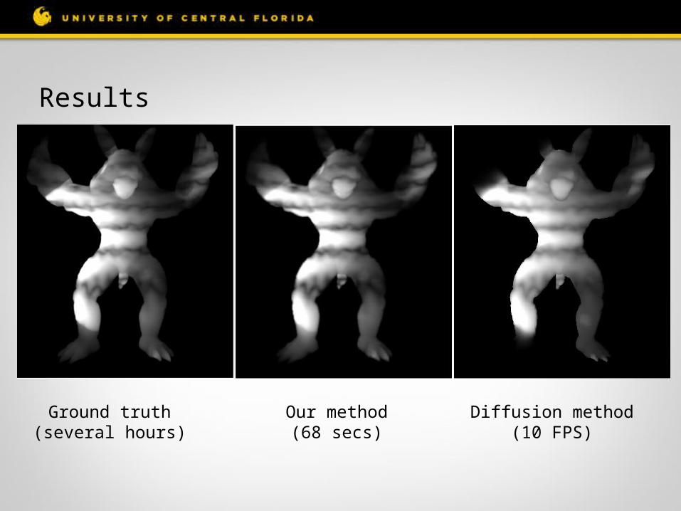
Results

Ground truth(several hours)

Our method(68 secs)

Diffusion method(10 FPS)

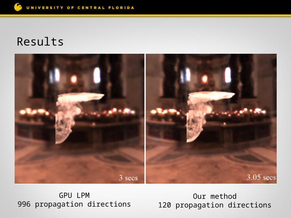
Results

GPU LPM996 propagation directions

Our method120 propagation directions

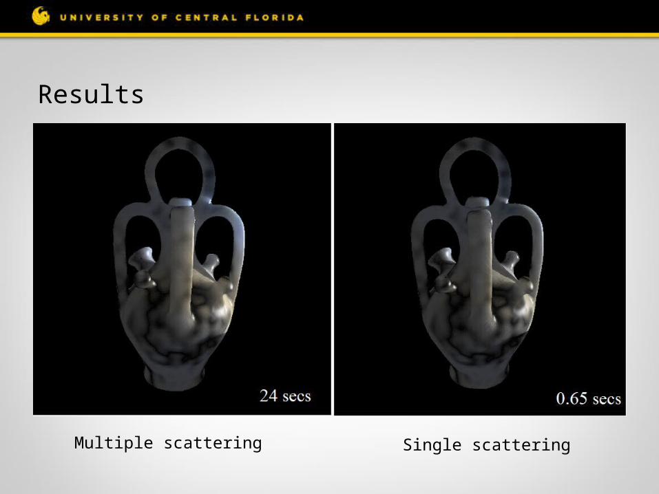
Results

Multiple scattering Single scattering

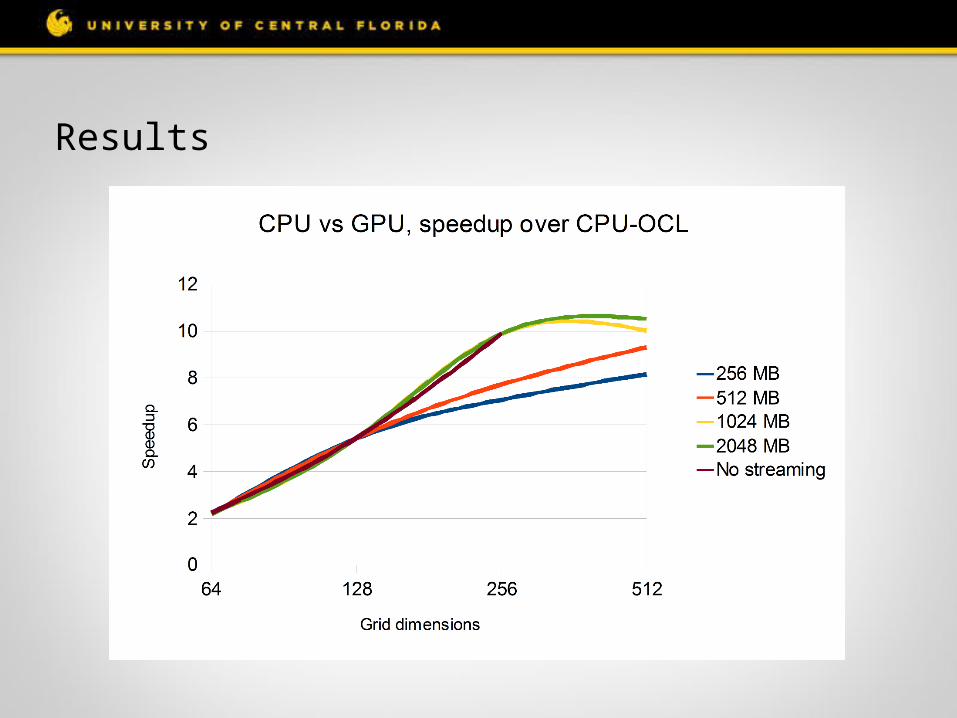
Results

Thank you