Parallel Matrix Multiplication - Cannon's Algorithm and 2 ...
48
Parallel Matrix Multiplication Cannon’s Algorithm and 2.5D Matrix Multiplication Charles and Dulac Thursday April 2, 2020
Transcript of Parallel Matrix Multiplication - Cannon's Algorithm and 2 ...

Parallel Matrix Multiplication
Cannon’s Algorithm and 2.5D Matrix Multiplication
Charles and Dulac
Thursday April 2, 2020
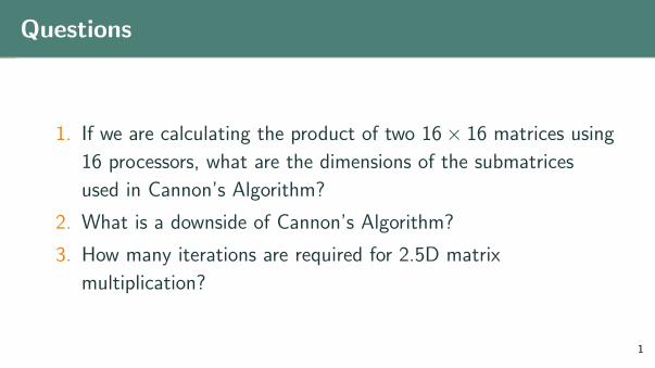
Questions
1. If we are calculating the product of two 16× 16 matrices using
16 processors, what are the dimensions of the submatrices
used in Cannon’s Algorithm?
2. What is a downside of Cannon’s Algorithm?
3. How many iterations are required for 2.5D matrix
multiplication?
1

Outline
Introductions
Parallelizing Matrix Multiplication
Cannon’s Algorithm
3D Matrix Multiplication
2.5D Matrix Multiplication
Summary
2

Introductions

Introduction: Liz Dulac
3

About Me: Liz Dulac
Major:
Physics
−→ [Applied] Mathematics (BS)
−→ Computer Science (BS)
Minor:
Fine Arts
−→ French
−→ Theatre (minor)
4

Hobbies: Theatre
5

Hobbies: Guard
6

The Bay State: Wicked Awesome
7

Amherst: Five College Consortium
8

The Bay State: Amherst
9
In Conclusion...
10

Introduction: MeiLi Charles
11

Maryville College
12

Hobbies: Cosplay
13

Meet my little friends
14
Parallelizing Matrix
Multiplication
Why Matrix Multiplication?
Applications
• Physics
• Graph theory
• Recurrence relations
• Tensors
15
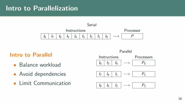
Intro to Parallelization
Serial
Instructions Processor
I8 I7 I6 I5 I4 I3 I2 I1 I0 −→ P
Intro to Parallel
• Balance workload
• Avoid dependencies
• Limit Communication
Parallel
Instructions Processors
I6 I3 I0 −→ P0
I7 I4 I1 −→ P1
I8 I5 I2 −→ P2
16
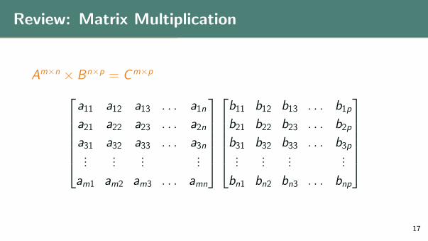
Review: Matrix Multiplication
Am×n × Bn×p = Cm×pa11 a12 a13 . . . a1na21 a22 a23 . . . a2na31 a32 a33 . . . a3n...
......
...
am1 am2 am3 . . . amn
b11 b12 b13 . . . b1pb21 b22 b23 . . . b2pb31 b32 b33 . . . b3p...
......
...
bn1 bn2 bn3 . . . bnp
17
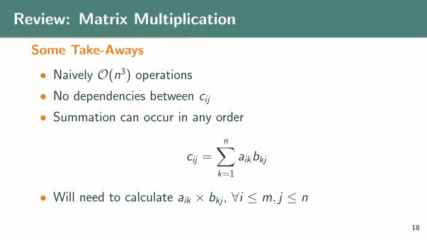
Review: Matrix Multiplication
Some Take-Aways
• Naively O(n3) operations• No dependencies between cij
• Summation can occur in any order
cij =n∑
k=1
aikbkj
• Will need to calculate aik × bkj , ∀i ≤ m, j ≤ n
18

Cannon’s Algorithm

Background
Cannon’s Algorithm
• Lynn Elliot Cannon
• Ph.D. Thesis, Montana State University,
14 July 1969
• A cellular computer to implement the
Kalman Filter Algorithm
19

Cannon’s Algorithm
Cannon’s Algorithm
• Each processor calculates
block of Cm×n
• Calculate one piece of dotproduct each iteration• Calculate index
k = (i + j + iter)(mod√p)
• Increment result by Aik × Bkj
P00 P01 P02 . . . P0√p
P10 P11 P12 . . . P1√p
P20 P21 P22 . . . P2√p
. . . . . . . . . . . . . . .
P√p0 P√
p1 P√p2 . . . P√
p√p
20

Cannon’s Algorithm: Example
Calculate: C 8×8 = A8×8 ∗ B8×8 using 16 processors.
• • • • • • • •• • • • • • • •• • • • • • • •• • • • • • • •• • • • • • • •• • • • • • • •• • • • • • • •• • • • • • • •
• • • • • • • •• • • • • • • •• • • • • • • •• • • • • • • •• • • • • • • •• • • • • • • •• • • • • • • •• • • • • • • •
21

Cannon’s Algorithm: Example
Processor Grid:
• 16 processors
=⇒ 4× 4 processor grid
P00 P01 P02 P03
P10 P11 P12 P13
P20 P21 P22 P23
P30 P31 P32 P33
22

Cannon’s Algorithm: Example
Processor Grid:
• 4× 4 processor grid
=⇒ 4× 4 block matrix dimensionsC00 C01 C02 C03
C10 C11 C12 C13
C20 C21 C22 C23
C30 C31 C32 C33
23
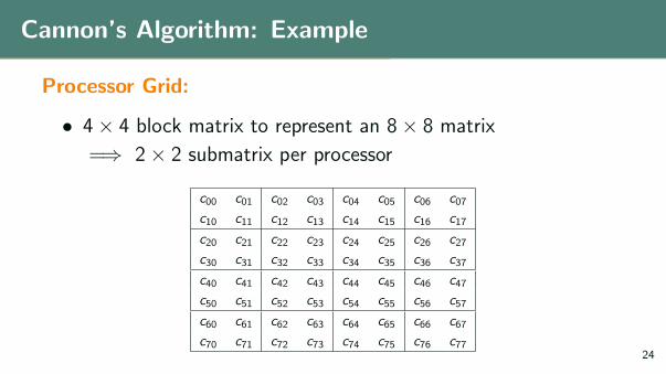
Cannon’s Algorithm: Example
Processor Grid:
• 4× 4 block matrix to represent an 8× 8 matrix
=⇒ 2× 2 submatrix per processor
c00 c01 c02 c03 c04 c05 c06 c07c10 c11 c12 c13 c14 c15 c16 c17
c20 c21 c22 c23 c24 c25 c26 c27c30 c31 c32 c33 c34 c35 c36 c37
c40 c41 c42 c43 c44 c45 c46 c47c50 c51 c52 c53 c54 c55 c56 c57
c60 c61 c62 c63 c64 c65 c66 c67c70 c71 c72 c73 c74 c75 c76 c77
24
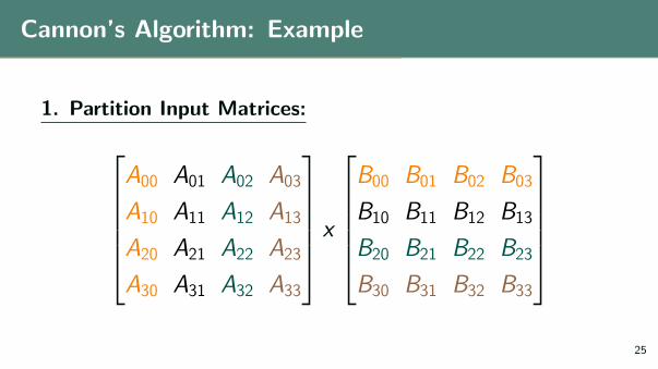
Cannon’s Algorithm: Example
1. Partition Input Matrices:A00 A01 A02 A03
A10 A11 A12 A13
A20 A21 A22 A23
A30 A31 A32 A33
x
B00 B01 B02 B03
B10 B11 B12 B13
B20 B21 B22 B23
B30 B31 B32 B33
25

Cannon’s Algorithm: Example
2. Pivot on Diagonals. Distribute to Processor Grid.
A00 A01 A02 A03
A11 A12 A13 A10
A22 A23 A20 A21
A33 A30 A31 A32
B00 B11 B22 B33
B10 B21 B32 B03
B20 B31 B02 B13
B30 B01 B12 B23
26

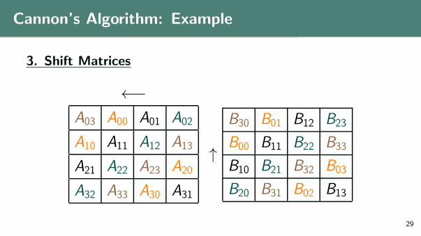
Cannon’s Algorithm: Example
3. Shift Matrices
←−A01 A02 A03 A00
A12 A13 A10 A11
A23 A20 A21 A22
A30 A31 A32 A33
↑
B10 B21 B32 B03
B20 B31 B02 B13
B30 B01 B12 B23
B00 B11 B22 B33
27

Cannon’s Algorithm: Example
3. Shift Matrices
←−A02 A03 A00 A01
A13 A10 A11 A12
A20 A21 A22 A23
A31 A32 A33 A30
↑
B20 B31 B02 B13
B30 B01 B12 B23
B00 B11 B22 B33
B10 B21 B32 B03
28
Cannon’s Algorithm: Example
3. Shift Matrices
←−A03 A00 A01 A02
A10 A11 A12 A13
A21 A22 A23 A20
A32 A33 A30 A31
↑
B30 B01 B12 B23
B00 B11 B22 B33
B10 B21 B32 B03
B20 B31 B02 B13
29

Cost
Time Space
O(n3/p) O(n2/p)
Note: redistributed matrices each of√p iterations
30

3D Matrix Multiplication

Cannon’s Algorithm −→ 3D
P P P P P
P P P P P
P P P P P
P P P P P
P P P P P
−→
P P P
P P P P
P P P P P
P P P P
P P P
Cannon (2D)
• n√p ×
n√p blocks
• √p Aij ∗ Bjk per processor
3D
• n3√p ×
n3√p blocks
• 1 Aij ∗ Bjk per processor
31

Cost
Time
• O(n3/p)Space
• O(n2/p2/3)
n2 mem/matrix copy ∗ 3√p copies /p processors
Communication Cost: only 1 iteration
32

What if we don’t QUITE have enough space for 3√p copies, but
would like to use the memory we do have?
33

2.5D Matrix Multiplication

Background
2.5D Matrix Multiplication
• Edgar Solomnik & James Demmel
• Communication-optimal parallel
2.5D matrix multiplication and LU
factorization algorithms
• Published in 2011
34

2.5D Matrix Multiplication
Goal:
• Take advantage of any extra memory to reduce amount of
communication
35

2.5D Matrix Multiplication
P P P P P P P P
P P P P P P P P P
P P P P P P P P P
P P P P P P P P P
P P P P P P P P P
P P P P P P P P P
P P P P P P P P P
P P P P P P P P P
P P P P P P P P
2.5D Copies
• Generalize to use
c copies
• c ∈ [1, 3√p]
36

Partitioning
Consider: square n × n matrices, p processors,
and c copies.
• pc processors per copy
•√
pc ×
√pc processor grid
• n√p/c× n√
p/cblocks
√pc
√pc
c11 c12 c13 . . . c1nc21 c22 c23 . . . c2nc31 c32 c33 . . . c3n...
......
...
cn1 cn2 cn3 . . . cnn
n
n
37
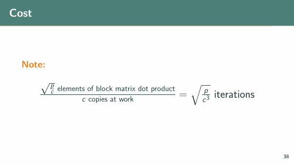
Cost
Note:
√pc elements of block matrix dot product
c copies at work =√
pc3
iterations
38

Summary

Summary
39

Questions?
40

Questions
1. If we are calculating the product of two 16× 16 matrices using
16 processors, what are the dimensions of the submatrices
used in Cannon’s Algorithm?
2. What is a downside of Cannon’s Algorithm?
3. How many iterations are required for 2.5D matrix
multiplication?
41