Parallel implementation of Apriori

algorithm and association of

mining rules using MPI Fall 2012

CSE 633- Parallel Algorithms

By,

Sujith Mohan Velliyattikuzhi

50027269

What is Apriori

• An efficient algorithm in data mining to find the

undiscovered relationships between different items.

• Operates on databases containing a set of

transactions with each transaction having a number

of item sets.

• Aims to find the set of “frequent item-sets” and

“association rules” between the items.

Frequent Item Sets

TID Items

1 Bread, Milk

2 Bread, Diaper, Beer, Eggs

3 Milk, Diaper, Beer, Coke

4 Bread, Milk, Diaper, Beer

5 Bread, Milk, Diaper, Coke

• An item set is a collection of one or more items. Eg {Bread,

Milk}

• Those items which occur more frequent.

• In other words, the item sets whose support is greater than the

given support.

Support and Support Count

• Support Count is the number of transactions

containing the itemsets. Eg – {Bread, Milk} = 3

• Support = Support Count/Total num of transactions

eg – {Bread, Milk} = 3/5 =0.6

• Frequent Item sets are those whose support is

greater than or equal to the specified support.

• It can be 1- itemset, 2-itemset… upto n-itemsets,

where n, is the total number of items.

Association rules

• Association rules is used for discovering interesting relationships among the items.

• Confidence of an association rule X-> Y = (# of transactions of X U Y ) /(# of transactions of X)

• An association rule is considered to be a strong association rule if its support and confidence are greater than the specified support and confidence.

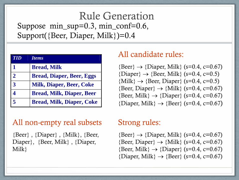
Rule Generation

TID Items

1 Bread, Milk

2 Bread, Diaper, Beer, Eggs

3 Milk, Diaper, Beer, Coke

4 Bread, Milk, Diaper, Beer

5 Bread, Milk, Diaper, Coke

All candidate rules:

{Beer} {Diaper, Milk} (s=0.4, c=0.67)

{Diaper} {Beer, Milk} (s=0.4, c=0.5)

{Milk} {Beer, Diaper} (s=0.4, c=0.5)

{Beer, Diaper} {Milk} (s=0.4, c=0.67)

{Beer, Milk} {Diaper} (s=0.4, c=0.67)

{Diaper, Milk} {Beer} (s=0.4, c=0.67)

Suppose min_sup=0.3, min_conf=0.6,

Support({Beer, Diaper, Milk})=0.4

Strong rules:

{Beer} {Diaper, Milk} (s=0.4, c=0.67)

{Beer, Diaper} {Milk} (s=0.4, c=0.67)

{Beer, Milk} {Diaper} (s=0.4, c=0.67)

{Diaper, Milk} {Beer} (s=0.4, c=0.67)

All non-empty real subsets

{Beer} , {Diaper} , {Milk}, {Beer,

Diaper}, {Beer, Milk} , {Diaper,

Milk}

The Apriori Algorithm

• Ck: Candidate itemset of size k

• Lk : frequent itemset of size k

• L1 = {frequent items};

• for (k = 1; Lk !=; k++) do • Candidate Generation: Ck+1 = candidates generated from Lk;

• Candidate Counting: for each transaction t in database do increment the count of all candidates in Ck+1 that are contained in t

• Lk+1 = candidates in Ck+1 with min_sup

• return k Lk;

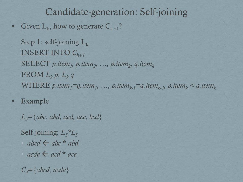
Candidate-generation: Self-joining

• Given Lk, how to generate Ck+1?

Step 1: self-joining Lk

INSERT INTO Ck+1

SELECT p.item1, p.item2, …, p.itemk, q.itemk

FROM Lk p, Lk q

WHERE p.item1=q.item1, …, p.itemk-1=q.itemk-1, p.itemk < q.itemk

• Example

L3={abc, abd, acd, ace, bcd}

Self-joining: L3*L3

• abcd abc * abd

• acde acd * ace

C4={abcd, acde}

Found to be

Infrequent

null

AB AC AD AE BC BD BE CD CE DE

A B C D E

ABC ABD ABE ACD ACE ADE BCD BCE BDE CDE

ABCD ABCE ABDE ACDE BCDE

ABCDE

Illustrating Apriori Principle null

AB AC AD AE BC BD BE CD CE DE

A B C D E

ABC ABD ABE ACD ACE ADE BCD BCE BDE CDE

ABCD ABCE ABDE ACDE BCDE

ABCDEPruned

Supersets

Level 0

Level 1

Output pattern of serial

implementation

• Number of transactions = 100 and different items = 200

Interesting patterns in the

output

• Output varies according to different inputs of

support and confidence and number of item sets

present.

• When the support is less, more time is taken to run

the program.

• As support increases, the time taken to run the

algorithm will be less and gradually comes to

constant after a point.

Challenges of apriori

algorithm

• More time is taken to generate output for low

support values.

• To discover a frequent pattern of size 100, about

2^100 candidates needed to generate.

• Multiple scans of database

• Solution ???? – Parallelize it.

Parallel implementation

• Divide the data sets.

• Each processor Pi will have its on data set Di

• Each processor Pi reads the values of the data set

from a large flat file.

• Each processor do calculation of count of item sets

in its own specific processing unit..

How it works

• Support and confidence are given as input to first

processor.

• First processor will broadcast the support and

confidence to every other processors.

• Each processor generates the first frequent item sets

from the input data.

• Then data is divided between different processors.

In subsequent passes

• Each processor Pi develops the complete Ck, using

the complete frequent itemset Lk-1 created at the end

of pass k-1

• Processor Pi develop local support counts for

candidates in Ck , using its local data partition.

• Then each processor Pi exchanges its local counts to

master processor to develop the global Ck counts.

Continued….

• Each processor Pi then computes Lk from Ck.

• Each processor Pi independently makes the decision

to terminate or continue to next pass.

• The decision will be identical as the processors have

all identical Lk.

Flow chart of parallel

implementation

Parallel rule generation

• Generating rules in parallel simply involves

partitioning the set of frequent item sets among the

processors.

• Each processor generates the rules using the below

algorithm

• If a rule Bread, Milk, Coffee->Diaper does not

satisfy the minimum confidence, then no need to

consider rules like Bread, Milk-> Coffee, Diaper.

MPI Commands used

• MPI_Comm_rank

• MPI_Bcast

• MPI_AllReduce

• Language used – C++

Test Cases

• Case 1 – To find the output pattern for different

values of support and constant number of

transactions

• Case 2 – To find the output pattern for different

number of transactions with same item sets.

• Case 3 – To find the output pattern for different item

sets with same number of transactions.

CASE 1

• Output value for different values of support.

• Both number of item sets and number of

transactions are kept constant.

• Various values of support from 40 to 70 are tested.

• Confidence is also kept constant at 50.

Output of parallel

implementation • Number of transactions =100, different number of items = 200.

• Confidence = 50

1 2 4 8 16 32 64 100 Freq.

Items

Assn

Element

s

40 184.815 139.554 69.596 36.438 19.628 12.244 9.578 7.882 1077 2528

45 16.1468 10.968 5.42 2.856 1.576 1.11 0.816 0.752 424 614

50 5.5649 3.762 1.866 0.98 0.552 0.346 0.318 0.282 174 138

55 0.9734 0.602 0.3 0.162 0.088 0.058 0.058 0.072 64 16

60 0.345 0.204 0.106 0.052 0.03 0.022 0.012 0.0216 36 4

65 0.1175 0.0616 0.031 0.015 0.008 0.014 0.016 0.0225 20 0

70 0.01932 0.01 0.005 0.002 0.001 0.0008 0.008 0.008 7 0

Time taken graph

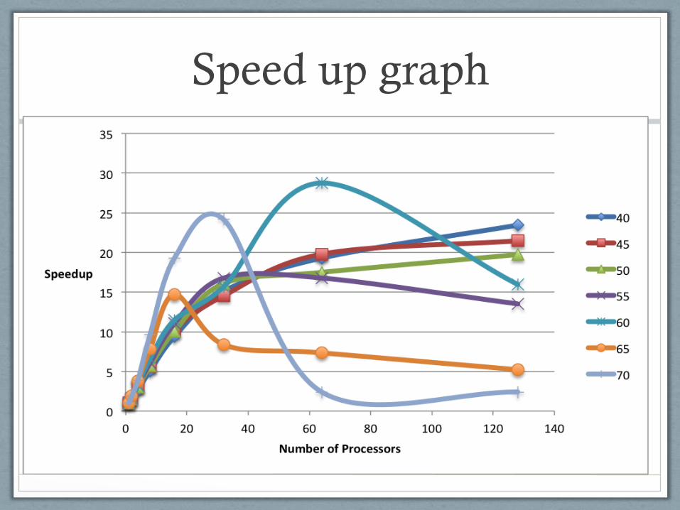
Speedup for parallel

implementation • Number of transactions =100, different number of items = 200.

• Confidence = 50

1 2 4 8 16 32 64 128

40 1 1.324 2.655 5.072 9.416 15.094 19.29 23.447

45 1 1.472 2.979 5.654 10.245 14.546 19.787 21.472

50 1 1.479 2.982 5.678 10.081 16.084 17.499 19.734

55 1 1.557 3.244 6.069 11.061 16.783 16.783 13.519

60 1 1.691 3.254 6.634 11.5 15.68 28.752 15.972

65 1 1.907 3.79 7.833 14.687 8.392 7.343 5.222

70 1 1.932 3.864 9.66 19.32 24.15 2.415 2.415

Speed up graph

Findings from case 1

• As the support increases, the time required to solve the problem will decrease.

• As number of processors increase, the time required to solve the problem will decrease and after some processors it becomes constant.

• In case of higher support, the time taken to solve the problem might increase when the number of processors. This is assumed to be due to the large number of communications happening, when compared to the time taken to solve the problem.

CASE 2

• Output for varying number of transactions

• Different transactions from 1000 to 64000 are taken.

• Support is kept at 55 and Confidence is kept at 50.

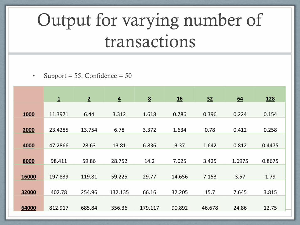
Output for varying number of

transactions

• Support = 55, Confidence = 50

1 2 4 8 16 32 64 128

1000 11.3971 6.44 3.312 1.618 0.786 0.396 0.224 0.154

2000 23.4285 13.754 6.78 3.372 1.634 0.78 0.412 0.258

4000 47.2866 28.63 13.81 6.836 3.37 1.642 0.812 0.4475

8000 98.411 59.86 28.752 14.2 7.025 3.425 1.6975 0.8675

16000 197.839 119.81 59.225 29.77 14.656 7.153 3.57 1.79

32000 402.78 254.96 132.135 66.16 32.205 15.7 7.645 3.815

64000 812.917 685.84 356.36 179.117 90.892 46.678 24.86 12.75

Time taken graph for different

number of transactions

Speed up table for varying

number of transactions

• Support = 55, Confidence = 50

1 2 4 8 16 32 64 128

1000 1 1.769 3.441 7.043 14.5 28.781 50.5879 74.007

2000 1 1.703 3.455 6.947 14.338 30.036 56.865 90.808

4000 1 1.652 3.424 6.917 14.032 28.798 58.234 105.668

8000 1 1.644 3.422 6.93 14.008 28.733 57.974 113.442

16000 1 1.651 3.34 6.645 13.498 27.658 55.417 110.524

32000 1 1.579 3.048 6.087 12.506 25.524 52.685 105.877

64000 1 1.185 2.28 4.53 8.943 17.415 32.69 63.758

Speed up graph for varying

number of transactions

Findings from case 2

• As the number of transactions increases, the time

taken to solve the problem will also increase.

• As the number of processors increases, the time

taken to solve the problem decreases and speed up

will also increase.

CASE 3

• Output for different number of item sets and with

same number of transactions

• Number of transactions is constant and kept at 1000

• Support = 70 and Confidence = 50

• Item sets having values between 200 and 800 are

tested.

Output for varying number of

item sets

• Support = 70, Confidence = 50, Number of transactions = 1000

1 2 4 8 16 32 64 128

200 0.1461 0.076 0.04 0.02 0.01 0.0075 0.008 0.01

400 1.2112 0.614 0.296 0.148 0.0729 0.038 0.03 0.02

600 2.086 1.05 0.525 0.265 0.135 0.065 0.045 0.03

800 21.2171 10.64 5.21 2.596 1.455 0.762 0.456 0.285

Time taken graph for different

item sets

Speed up table for varying

number of item sets

• Support = 70, Confidence = 50, Number of transactions = 1000

1 2 4 8 16 32 64 128

200 1 1.921 3.65 7.3 14.6 18.25 18.25 14.6

400 1 1.972 4.091 8.182 16.589 31.868 40.366 60.55

600 1 1.986 3.973 7.87 15.45 32.09 46.35 69.55

800 1 1.994 4.072 8.174 14.58 27.91 46.64 74.44

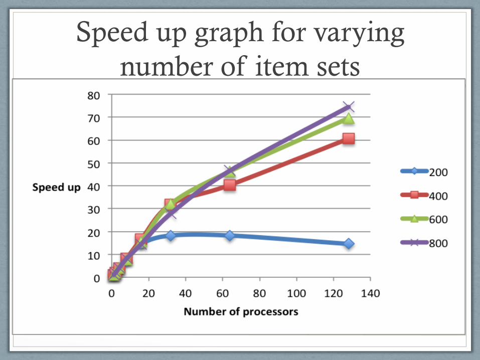
Speed up graph for varying

number of item sets

Findings from case 3

• As the number of item sets increases, the time taken

to run the program will increase.

• Since high value of support is used, the time taken to

run the program might increase when number of

processors increases.

• This is mainly because of the large amount of

communication happening in the program.

Conclusions

• Was able to identify the benefits of parallelizing.

• When number of processors was increased,

corresponding reduction in time taken was clearly

seen.

• The output depends on the size as well as the type of

input data.

Future Work

• To implement apriori algorithm using Open MP and

compare its performance with MPI implementation

of the same.

References

1. http://rakesh.agrawal-

family.com/papers/tkde96passoc_rj.pdf

2. http://www.cse.buffalo.edu/faculty/azhang/cse60

1/