University of Nebraska at OmahaDigitalCommons@UNO

Student Work

5-2012

Parallel Adaptive Algorithms for Sampling LargeScale NetworksKanimathi DuraisamyUniversity of Nebraska at Omaha

Follow this and additional works at: https://digitalcommons.unomaha.edu/studentwork

Part of the Computer Sciences Commons

This Thesis is brought to you for free and open access byDigitalCommons@UNO. It has been accepted for inclusion in StudentWork by an authorized administrator of DigitalCommons@UNO. Formore information, please contact unodigitalcommons@unomaha.edu.

Recommended CitationDuraisamy, Kanimathi, "Parallel Adaptive Algorithms for Sampling Large Scale Networks" (2012). Student Work. 2872.https://digitalcommons.unomaha.edu/studentwork/2872

Parallel Adaptive Algorithms for Sampling

Large Scale Networks

A Thesis Presented to the

Department of Computer Science and the Faculty of the Graduate College

University of Nebraska

In Partial Fulfillment of the Requirements for the Degree

Masters of Science

University of Nebraska at Omaha

By

Kanimathi Duraisamy

May, 2012

Supervisory Committee

Dr. Sanjukta Bhowmick, Chair Dr. Hesham Ali

Dr. Parvathi Chundi Dr. Dhundy Bastola

All rights reserved

INFORMATION TO ALL USERSThe quality of this reproduction is dependent on the quality of the copy submitted.

In the unlikely event that the author did not send a complete manuscriptand there are missing pages, these will be noted. Also, if material had to be removed,

a note will indicate the deletion.

All rights reserved. This edition of the work is protected againstunauthorized copying under Title 17, United States Code.

ProQuest LLC.789 East Eisenhower Parkway

P.O. Box 1346Ann Arbor, MI 48106 - 1346

UMI 1508621Copyright 2012 by ProQuest LLC.

UMI Number: 1508621

Parallel Adaptive Algorithms for Sampling Large Scale Networks

Kanimathi Duraisamy, MS

University of Nebraska at Omaha, 2012

Advisor: Dr.Sanjukta Bhowmick

Abstract

The study of real-world systems, represented as networks, has important

application in many disciplines including social sciences [1], bioinformatics [2] and

software engineering [3]. These networks are extremely large, and analyzing them is very

expensive. Our research work involves developing parallel graph sampling methods for

efficient analysis of gene correlation networks. Our sampling algorithms maintain

important structural and informational properties of large unstructured networks. We

focus on preserving the relative importance, based on combinatorial metrics, rather than

the exact measures. We use a special subgraph technique, based on finding triangles

called maximal chordal subgraphs, which maintains the highly connected portions of the

network while increasing the distance between less connected regions. Our results show

that even with significant reduction of the network we can obtain reliable subgraphs

which conserve most of the relevant combinatorial and functional properties.

Additionally, sampling reveals new functional properties which were previously

undiscovered in the original system.

Keywords: chordal graphs, parallel graph sampling, correlation networks, noise

reduction, cluster overlap, edge enrichment score

i

Acknowledgements

It gives me great pleasure in acknowledging the support and help of my advisor

Dr.Sanjukta Bhowmick who offered me invaluable assistance, encouragement, guidance

and support throughout my thesis work. One simply could not wish for a better,

friendlier and supportive mentor who could guide me through completion of this

research. I am heartily thankful to Dr.Hesham Ali, without his knowledge and assistance

this thesis would not have been successful. I am also grateful to Dr. Dhundy Bastola and

Dr.Parvathi Chundi for all their constructive comments and valuable suggestions for my

thesis work. I share the credit of my work with Ms. Kathryn Dempsey who helped me in

obtaining the biological functional units.

My deepest gratitude goes to my family especially to my sister and brother-in-

law, this research would have been simply impossible without their support and

encouragement. I really want to thank all my family members for all their motivation and

encouragement in all the areas of my life. I love to thank all my friends who where always

there and supported me through this thesis.

ii

Table of Contents

1. Introduction...................................................................................................................1

1.1 Outline of Thesis................................................................................................2

2. Background....................................................................................................................4

2.1 Graph Terminology............................................................................................4

2.2 Sampling............................................................................................................6

2.3 High Performance Computing..........................................................................8

2.4 Gene Correlation Networks..............................................................................8

3. Algorithm Description......... …...................................................................................10

3.1 Data Structure..................................................................................................12

3.2 Chordal Graph Based Sampling.......................................................................14

3.2.1 Parallel Algorithm with Communication..........................................15

3.2.2 Parallel Algorithm without Communication.....................................18

3.3 Random Walk Based Sampling.......................................................................19

4. Analysis of Results.......................................................................................................21

4.1 Analysis of Combinatorial Properties..............................................................21

4.2 Analysis of Functional Properties....................................................................26

4.2.1 Analysis of Different Ordering.........................................................30

4.2.2 Analysis of Quality of Clusters.........................................................34

4.3 Analysis of Parallel Results.............................................................................41

5. Conclusion....................................................................................................................44

References.........................................................................................................................45

iii

List of Figures

Figure 2.1: Example of Undirected Graph.........................................................................4

Figure 2.2: Visual representation of graphs and their associated sampled subgraphs.......7

Figure 3.1: CSR format for a network.............................................................................13

Figure 3.2: Original graph and it's maximal chordal subgraphs(sequential)...................14

Figure 3.3: Original graph and it's maximal chordal subgraphs(parallel)........................15

Figure 3.4: Visualization of networks for creatine mice dataset......................................16

Figure 3.5: Breakdown of execution time for obtaining QCS over different number of processors.......................................................................................................17 Figure 3.6: Gene expression networks of the hypothalamus of a mouse brain and their respective Chordal graph representations.......................................................19 Figure 4.1: Degree distribution and average clustering coefficient of middle aged mice dataset...........................................................................................................25 Figure 4.2: Degree distribution and average clustering coefficient of young mice dataset............................................................................................................25 Figure 4.3: Degree distribution and average clustering coefficient of creatine mice dataset............................................................................................................26

Figure 4.4: Degree distribution and average clustering coefficient of untreated mice dataset………………………………………………………………………26 Figure 4.5: Comparison of functional units of young mice dataset.................................27

Figure 4.6: Comparison of functional units of middle aged mice dataset.......................28

Figure 4.7: Comparison of functional units of creatine mice dataset..............................29

Figure 4.8: Comparison of functional units of untreated mice dataset............................30

Figure 4.9: Gene functionality of clusters for the young mice dataset with BFS ordering………………………………………………………………….....32 Figure 4.10: Gene functionality of clusters for the young mice dataset with RCM ordering.......................................................................................................33

iv

Figure 4.11: Example of how network sampling can positively or negatively affect the average edge enrichment score of a cluster by removing different sets of edge….........................................................................................................35 Figure 4.12: Example of how to identify the likely biologically meaningful cluster…...37 Figure 4.13: Node and edge overlap for original vs. sampled networks .........................38

Figure 4.14: Newly discovered nodes and edges for original vs. sampled networks......38

Figure 4.15: Sensitivity and specificity of filters for node and edge overlap...................39

Figure 4.16: Example of how filtering impacts a cluster..................................................41

Figure 4.17: Scalability of sampling algorithms for a young and creatine mice network42

Figure 4.18: Parallel results for creatine natural order filter.............................................43

v

List of Tables

Table 4.1: Comparison of combinatorial properties between the original network and chordal subgraphs………................................................................................23 Table 4.2: Comparison of combinatorial properties between the original network and random walk subgraphs..................................................................................24

1

Chapter 1

Introduction

A network is a set of vertices and edges and has proved to be a useful abstraction

for solving real world problems arising in systems of interacting entities. In a network

model vertices represent the entities and the edges represent interactions, flow of

information, degree of similarity or social relations between them. An advance in data

collection, storage and retrieval has led to a proliferation of very large networks.

However analyzing these networks, that is computing graph theoretic properties of the

network and then relating them to the functionalities of underlying system, is a

challenging task.

The underlying purpose of network analysis is to extract meaningful data from an

application. However for large scale networks (Facebook has 8 million users) analysis

process is both computation and memory intensive. Two popular techniques for reducing

the use of resources are (i) using high performance computing to divide data over

multiple processing units[4,5,6] (ii) sampling[7,8,9] that is extracting representative

subgraph that exhibits similar characteristics to the original larger network.

A more insidious problem concerns noise in networks. Real-world networks are

built using experimental (such as gene correlation networks) or subjective (census

reports, epidemic distribution) techniques. The fluctuations and bias inherent in these

methods would also be present in the form of small errors or noise within the network

models. Let us take the famous example Facebook. The facebook algorithm suggests that

you might know a person, because you have four mutual friends, which can be a good

2

predictor of direct relationship. But sometimes Facebook can get it wrong because that

person might be somebody whom you didn't met in your life. Such miscalculation occurs

because not all connections in the Facebook are not of equal importance. Assuming equal

importance to all edges is a form of noise. Once again selective sampling based on the

analysis objective can reduce the noise in networks.

In this thesis, we developed scalable parallel network sampling algorithms that

can filter out the noise, while preserving the important characteristics of the network. We

compared two sampling techniques that are random walk and maximal chordal subgraph

along with different permutations of the original network.

Our strategy is unique in that in contrast to other network filtering algorithms

which only compare structural properties, whereas we compare both structural and

functional properties. We validate our methods by using them to analyze gene correlation

networks arising in murine models. Reduction of noise provides additional insight to the

functional properties of the underlying application.

Our results show that chordal graph based sampling not only conserves clusters

that are present within the original networks, but by reducing noise can also help uncover

additional functional clusters that were previously not identifiable from the original

network. We extend our research to investigate how different orderings affect the results

of our sampling, and maintain the viability of resulting network structures. We show that

our network sampling filter is a much better approach compared with other sampling

filter like random walk.

3

1.1 Outline of Thesis:

This thesis is organized as follows. In Chapter 2, we provide brief overview and

recent work in graph sampling. In Chapter 3, we describe our implemented newly

developed parallel algorithm. In Chapter 4, we present our experimental results and

analysis which include comparing both combinatorial and functional properties of

original network and subnetworks. In Chapter 5, we discuss our concluding remarks and

present potential ideas for further research.

4

Chapter 2

Background

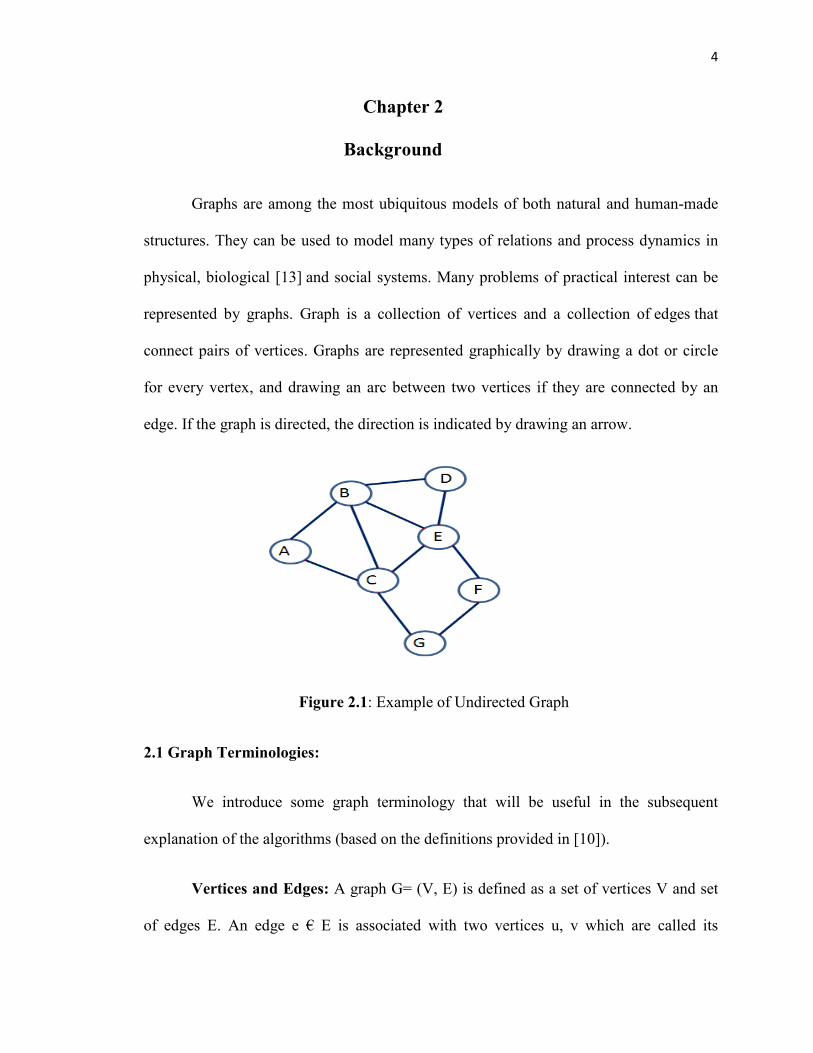
Graphs are among the most ubiquitous models of both natural and human-made

structures. They can be used to model many types of relations and process dynamics in

physical, biological [13] and social systems. Many problems of practical interest can be

represented by graphs. Graph is a collection of vertices and a collection of edges that

connect pairs of vertices. Graphs are represented graphically by drawing a dot or circle

for every vertex, and drawing an arc between two vertices if they are connected by an

edge. If the graph is directed, the direction is indicated by drawing an arrow.

Figure 2.1: Example of Undirected Graph

2.1 Graph Terminologies:

We introduce some graph terminology that will be useful in the subsequent

explanation of the algorithms (based on the definitions provided in [10]).

Vertices and Edges: A graph G= (V, E) is defined as a set of vertices V and set

of edges E. An edge e € E is associated with two vertices u, v which are called its

5

endpoints. A vertex u is said to be a neighbor of vertex v, if they are joined by an edge. In

Figure 2.1, there are total 7 vertices and 10 edges in the graph.

Cycle: A Path is an alternating sequence of vertices and edges, where subsequent

vertices are connected by an edge. A Cycle is a path where the initial and final vertices

are identical. In Figure 2.1, vertices (A, B, E, C, A) forms cycle.

Clique: A Clique is a set of vertices that are all connected to each other. In Figure

2.1, vertices (A, B, C) forms clique because everyone in the group is connected to each

other. Some other cliques are (B, E, C) and (B, E, D).

Degree: Degree of a vertex in a graph is the number of edges the vertex has with

the other vertices. The Degree of vertex v is denoted as deg(v). Vertices with high

degrees are called hubs. In Figure 2.1, Degree of vertices are, deg(A) = 2 , deg(B) = 4,

deg(C) = 4, deg(D) = 2, deg(E) = 4, deg(F) = 2 and deg(G) = 2.

Degree Distribution: Degree Distribution is the probability distribution of

degrees of the vertices over the network. Degree distribution is (d1, d2… dn-1), where dk is

the number of vertices with degree k. Degree Distribution for graph in Figure 2.1 is (0, 4,

0, 3, 0). Most scale free system like social and biological networks observe a power law

based distribution [29] that is there are many vertices with low degree and the number of

vertices exponentially go down as the degree increases.

Clustering Coefficient: Clustering Coefficient is a measure of degree to which

nodes in a graph tend to cluster together. It is calculated as the ratio of the edges between

the neighbors of a vertex to the total possible connection between them. The higher the

clustering coefficient it is more likely that a vertex is part of a dense module with closely

6

interconnected dependencies. In Figure 2.1, Clustering Coefficients values of vertex A =

1, vertex B = 0.5, vertex C = 0.3, vertex D = 1.0, vertex E = 0.3, vertex F = 0, vertex G =

0.

Core Number Distribution: Core Number of a vertex is defined as the largest

integer c such that the vertex exists in a graph where all degrees are greater than equal to

c. The higher the value, the better the clustering property should be maintained. In Figure

2.1, Core Number of all vertices is 2.

Chordal Graph: A Chordal Graph is a graph where the length of a cycle is be no

more than three.

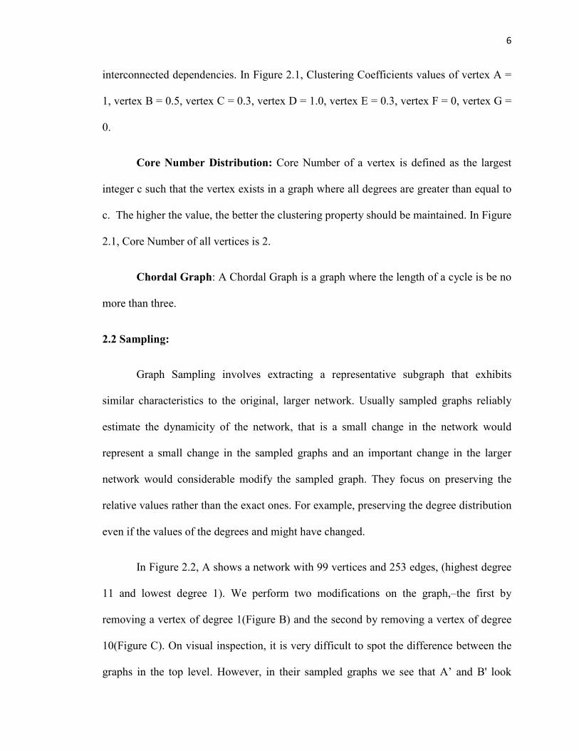
2.2 Sampling:

Graph Sampling involves extracting a representative subgraph that exhibits

similar characteristics to the original, larger network. Usually sampled graphs reliably

estimate the dynamicity of the network, that is a small change in the network would

represent a small change in the sampled graphs and an important change in the larger

network would considerable modify the sampled graph. They focus on preserving the

relative values rather than the exact ones. For example, preserving the degree distribution

even if the values of the degrees and might have changed.

In Figure 2.2, A shows a network with 99 vertices and 253 edges, (highest degree

11 and lowest degree 1). We perform two modifications on the graph,–the first by

removing a vertex of degree 1(Figure B) and the second by removing a vertex of degree

10(Figure C). On visual inspection, it is very difficult to spot the difference between the

graphs in the top level. However, in their sampled graphs we see that A’ and B' look

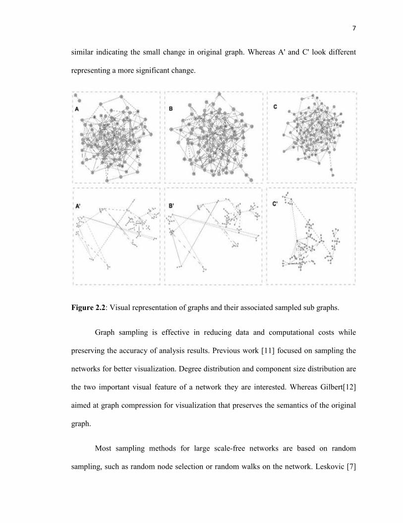
7

similar indicating the small change in original graph. Whereas A' and C' look different

representing a more significant change.

Figure 2.2: Visual representation of graphs and their associated sampled sub graphs.

Graph sampling is effective in reducing data and computational costs while

preserving the accuracy of analysis results. Previous work [11] focused on sampling the

networks for better visualization. Degree distribution and component size distribution are

the two important visual feature of a network they are interested. Whereas Gilbert[12]

aimed at graph compression for visualization that preserves the semantics of the original

graph.

Most sampling methods for large scale-free networks are based on random

sampling, such as random node selection or random walks on the network. Leskovic [7]

8

stated that random walks and forest fire are good at extracting samples from large

networks. They are interested in finding a general sampling method that would match a

full set of graph properties. A recent work [14] analyze the result of various sampling

algorithms using three different measures namely Degree, Clustering and Reach. Most of

the previous work concerned with constructing samples that match structural properties

of the original network.

A parallel version of random walks is based on starting multiple walks

simultaneously on different processors [15]. Parallel algorithms for obtaining spanning

trees such as breadth first trees, connected components and minimum spanning trees on

large-scale networks are also being investigated [4,5,6].However the spanning tree

methods focus more on graph traversal than sampling important regions.

Filtering noise for large networks is still a largely unaddressed problem Some

recent work has focused [16,17] on using machine learning techniques to detect noise in

biological networks and uses supervised learning to predict noise based on prior

information.

Our algorithm effectively select good representative samples of a large graph that

can filter out the noise, while preserving important characteristics of the network so that

sampled graphs can be used for more complicated experiments.

2.3 High Performance Computing:

With the increase in data and problem sizes, high performance computing has

become an essential tool for efficient implementation of large scale applications. In the

sequential programming, processes are run one after another in a succession fashion and

9

it's expensive. In high performance computing, we have multiple processes execute at the

same time and so we can complete time consuming operation in less time.

2.4 Gene Correlation Networks:

A correlation network is represented as a graph, where vertices represent genes

and edges represent the correlation between the expression levels of two genes. Gene

correlation networks are created based on the correlation between expression levels of

different genes as obtained from microarray data analysis. Different measurements of

correlation have been used to build these networks, such as the partial correlation

coefficient [19], the Spearman correlation coefficient [20] and more commonly, the

Pearson correlation coefficient [21].There are many methods for thresholding the

correlation network. The most straightforward involves removing edges with a low

correlation. In a larger network created using the Pearson correlation coefficient, we use a

threshold of ±0.70 to ±1.00 based on the fact that the coefficient of determination for

these correlations will be at least 0.49.

The degree distribution of correlation networks follows a power-law distribution

[22] that indicates a scale-free network structure. Adherence to this distribution indicates

that there are many nodes in the network that are poorly connected and a few nodes that

are very well connected; these nodes are known as "hubs”. A primary analytical

operation of correlation networks is identifying high density clusters of genes,

represented by tightly connected vertices in the network. Analyzing these networks is a

computationally expensive which creates the need for efficient sampling mechanisms.

Furthermore, correlation networks can have noise or unnecessary edges, which can

adversely impact the accuracy of the results.

10

Chapter 3

Algorithm Description

Graph sampling should represent the relevant features of the larger network

especially structural and informational properties that helps to improve the interpretation

of large networks. Moreover, sampling is effective in reducing computational and data

costs and also the sampled subgraph occupies less memory than original network. The

objective of our sampling algorithm is to maintain the highly connected subgraphs like

cliques from the original network while removing some of the associated noise. We

assume that the effect of noise is more likely to be prevalent in structures formed by

loosely connected vertices. Spanning subgraphs which includes all the vertices and some

edges of the graph such as Minimum Spanning Tree, Steiner Tree, Planar Tree, Random

Walk and Chordal Subgraphs possess many of the these properties to sample a graph

perfectly.

For a given graph/network, Minimum/Maximum Spanning Tree (MST) is a

subset of all edges that connects all nodes at minimum/maximum total weight without

cycles. The heaviest edge in any cycle cannot be in the minimal spanning tree. Moreover,

the lightest edge in any cut must be in the minimal spanning forest. so we cannot

guarantee that all the important functional properties would be retained in sampled graph.

In addition, all the cycles will be deleted in spanning tree which means it can't keep

densely connected regions.

11

Steiner Tree problem is superficially similar to the Minimum Spanning

Tree problem: given a set V of points (vertices), interconnect them by a network (graph)

of shortest length, where the length is the sum of the lengths of all edges. The difference

between the Steiner Tree problem and the Minimum Spanning Tree problem is that, in

the Steiner Tree problem, extra intermediate vertices and edges may be added to the

graph in order to reduce the length of the spanning tree. Adding more information to the

Steiner Tree distort the values present already present in network.

Planar Graph is a graph which can be drawn in the plane (e.g. on a piece of

paper) without any of the edges crossing over, that is, meeting at points other than

the vertices. Several important graph theoretic concepts were discovered by looking at

planar graphs. The notion of vertex coloring of graphs came from the four color

conjecture about planar graphs. Similarly, Hamiltonian paths and cycles were studied for

planar graphs. But if the original network has clique of 5 or a complete bipartite graph

with 3 nodes on each side, then subgraph will not be retained in sampled graphs. We

found it is difficult to retain almost all densely connected regions in planar graph.

In the recent years, many researchers have focused on random walk in graph

sampling area [7]. A Random Walk selects the next node at random from among the

neighbors of the current node. Random Walk has a good chance of finding densely

connected regions in large network. This motivated us to do some background research

on this area and write parallel code to extract a subgraph from the larger network. As

expected, sampled subgraphs find clusters from larger network. We went a step ahead

12

and analyze the quality of those clusters. Unfortunately, the sampled graph using Random

Walk did not retain the important biological properties.

Chordal Subgraph is a spanning subgraph of the network where there are no

cycles of length larger than three. This interesting family of graphs is not only good for

sampling, but Chordal Subgraphs preserve many topological features such as the number

of triangles, the number of cliques, and the lower bound on the number of colors. Choices

of edges to be retained in Chordal graphs are based on information content which

indicates that sampling based on Chordal graphs will retain important informational

properties of the network. Due to these properties of the Chordal graphs, they can be used

to construct efficient linear time algorithms for non-polynomial problems such as

minimum coloring and maximum cliques. It provides the approximation of the larger

graph to obtain near exact results with low computational cost and also the complexity of

finding Chordal Subgraph is O(|E|*max_deg)[18]. Retrieving Maximum Chordal

Subgraph from the given network is NP hard problem so we decided to go with Maximal

Chordal Subgraph based on the algorithm provided by Dearing et. al.[18] to maintain the

densely connected regions in the sampled subgraph.

3. 1 Data Structure:

Compressed row storage method [33] is a popular format for representing

elements of sparse matrices. The storing the non-zero elements of a sparse matrix into a

linear array is done by walking down each column or across each row in order, and

writing the non-zero elements to a linear array in the order they appear in the walk.

13

Graphs can be represented as an adjacency matrix where rows and columns are labeled

by graph vertices and value of adjacency matrix (Vi, Vj) is 1 if there is an edge between

vertex Vi and vertex Vj otherwise 0 . In this method all the information is stored into three

vectors as described below.

(a)Values: stores the non-zero values of a sparse matrix by walking down each column

and writing a non-zero values

(b) Columns: Value of Columns[i] is the number of the column of adjacency matrix that

contains the Values[i] element.

(c) Row Index: Value of Row Index[i] gives the index of the element of the Values array

of the first non-zero element in a row ‘i’ of adjacency matrix.

(a) (b)

(c)

Figure 3.1 CSR format for a network a) The original network of 5 vertices b) The sparse adjacency matrix corresponding to the network. c) The CSR format for the sparse matrix

14

3.2 Chordal Graph Based Sampling:

Our sampling technique for obtaining the maximal chordal subgraph is provided

by Dearing et. al. [18]. This method is based on growing the graph from a starting vertex

and adding edges as long as they maintain the chordal characteristics. Initially the chordal

subgraph consists of the starting vertex and its associated edges. In the subsequent steps,

the vertex with the maximum number of visited neighbors is selected. An edge from the

current selected vertex a, (a,b) is added to the chordal subgraph if the number of visited

neighbors of b is a subset of the number of visited neighbors of a. The complexity of this

algorithm is O(Ed) where E is the number of edges in the graph and d is the maximum

degree.

Figure 3.2: Original Graph (Left) and it maximal chordal subgraph(Right )

The sequential algorithm for finding MCS and indeed most of the sampling

methods assume that the original network is connected. However, many real-world

15

networks, such as our test suite of gene correlation networks have disconnected

components. Based on our initial tests, we discovered that a completely chordal subgraph

is a very strict restriction, and can disintegrate some clusters, that are almost, but not

exact, cliques. To counteract this effect we modified the algorithm to extract quasi-

chordal subgraphs, which can include few cycles of length greater than three. We believe

that more loosely coupled structures are potentially eliminated in quasi chordal subgraph

by including only border edges that are part of at least one triangle. In order to

accommodate large networks, we have developed and implemented a parallel algorithm

for extracting the maximal chordal subgraphs from the network. These subgraph

preserves most of the cliques and highly connected regions of the network which

increases the path lengths between loosely connected regions. We validate our algorithms

by applying them to analyze gene correlation networks.

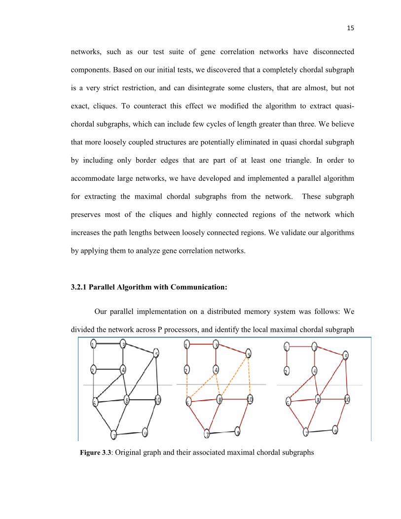
3.2.1 Parallel Algorithm with Communication:

Our parallel implementation on a distributed memory system was follows: We

divided the network across P processors, and identify the local maximal chordal subgraph

Figure 3.3: Original graph and their associated maximal chordal subgraphs

16

formed only of the edges whose endpoints lie completely within a processor. Next, we

identify the border edges whose endpoints lie across the partitions. For each pair of

processors we identified a receiver where the synchronization would take place. We

assign the processors as sender and receiver in such a way that computation load is

balanced across all processors. We sent the border edges to designated receiver

processors. The edges that lie across processors is included only if two

border edges with a common vertex combined with a previously marked chordal edge to

form a triangle. This implementation generated quasi-chordal subgraphs (QCS), since the

inclusion of border edges can sometimes increase the length of cycles by more than three.

Figure 3.4: Visualization of networks from the creatine treated mice. A: Original Network. B: QCS with 1 Partition: QCS with 2 Partitions. D: Left Figure: QCS with 4 Partitions. E: QCS with 8 Partitions. F: QCS with 16 Partitions.

Figure 3.4 shows the QCS generated from one of our sample networks. The

scalability of our parallel algorithm can be computed as follows; Let the number of edges

17

in the network be E, the maximum degree of the network be d and the number of

processors involved be p. The complexity of the sequential algorithm is given by Tseq(E)

= O(Ed). The parallel overhead Tover(E,p) consists of communicating the border nodes

from each processor, denoted by b, and subsequently checking, for each pair of border

nodes, if they form a triangle with a chordal edge. Assuming equal distribution of border

nodes, the total communication volume is O(bp) and the computation volume over all

processors is O(b2p). Therefore, Tover(E,p) = O(b2p). In order maintain isoefficiency,

Tseq(E)>=Tover(E,p), which implies E >=Cb2p/d, where C is a constant. The memory

required by to store the network is approximately O(E). Therefore, the scalability

function for this algorithm can be computed as (Cb2p)/(dp) = O(b2/d). Thus, the parallel

overhead increases with the number of border edges.

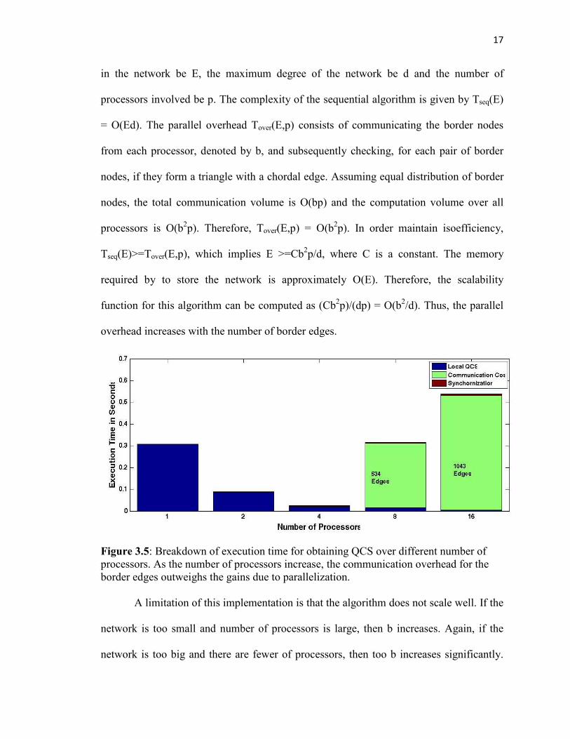
Figure 3.5: Breakdown of execution time for obtaining QCS over different number of processors. As the number of processors increase, the communication overhead for the border edges outweighs the gains due to parallelization. A limitation of this implementation is that the algorithm does not scale well. If the

network is too small and number of processors is large, then b increases. Again, if the

network is too big and there are fewer of processors, then too b increases significantly.

18

Additionally, depending on the distribution some processors might have more border

edges to analyze as compared to other processors.

Figure 3.5 shows the breakdown of the execution times of the different sections of

the algorithm over 1,2,4,8 and 16 processors. As can be seen from the figure the time to

compute the local QCS (blue blocks) gradually decreases over the number of processors.

However, the communication costs (border edges) keep increasing with the number of

processors, which finally leads to significant increase in the execution time.

3.2.2 Parallel Algorithm without Communication

Primary goal is to reduce the communication costs and maintain a better balance

of the workload.

In this version, graph is partitioned as before, and then chordal edges and border

edges are marked. Instead of sending the border edges to the receiver, we simply compare

them with the local chordal edges. Pair of border edges is included in the subgraph if they

form a triangle with already marked chordal edge. In Figure 1, edges (2, 6) and (4, 6) will

not be included in the top partition because (2, 4) is not a chordal edge. However in the

bottom partition (4, 6) and (4, 8) are included since (6, 8) is a chordal edges and so are (5,

8) and (5, 10). This implementation requires no communication and provides a more

equitable distribution of the workload. It is therefore more scalable than our earlier

algorithm.

Because multiple processors can work on the same border edge, it is likely that

some of the border edges will be represented twice in the final filtered subgraph. During

19

analysis, which is done sequentially, we have to remove these duplications. In the worst

case there can be as many as b duplications, where b is the number of border edges.

Figure 3.6: Gene expression network of the hypothalamus of a mouse brain with larger components highlighted in broken line boxes (A-D) and the respective chordal graph representations shown below (A’-D’). The chordal graphs preserve the structure but have significantly lower number of edges.

Our primary contribution is in developing a parallel sampling technique for large-

scale networks that not only extracts important combinatorial properties, but also

eliminates some of the inherent noise in the networks. Reduction of noise provides

additional insight to the functional properties of the underlying application. Figure 3.6

20

demonstrates how QCS based sampling can effectively select good representative

samples of a large graph.

3.3 Random Walk Based Sampling:

In order to compare the effectiveness of our method, we also implemented a

parallel random filtering method. The random walk was also designed as a variation on

graph traversal. At each vertex of degree d, one of its associated edges was selected with

probability 1/d. The graph traversal was completely random in that we did not maintain a

list of which edges or vertices have been visited, and a vertex could be visited multiple

times. The rationale for random walk is that tightly connected groups of vertices will

have a higher chance of being repeatedly selected and therefore cliques and other highly

connected regions would be preserved in the filtered graph. The traversal process is

continued iteratively until the number of times edges are selected is half the total number

of edges in the network.

The parallel random walk algorithm also divides the network across processors

and as in the case of the chordal graph based sampling, each processor finds its local

random walk based subgraph. Each border edge is associated with a binary random value,

and based on the value the edge is either included in the subgraph (e.g. for value 1) or not

(e.g. for value 0). However, the addition of the border edges is much simpler. This

algorithm is of course perfectly scalable as again no communication is required for the

border edges. The random walk filter would also require less execution time than the

chordal graph filter, because the choice of the next edge is much simpler.

21

Chapter 4

Analysis of Results

The datasets GSE5140 and GSE5078 for our experiments were obtained from

NCBIs Gene Expression Omnibus (GEO) website (http://www.ncbi.nlm.nih.gov/geo/)

and divided based on age/treatment [23, 24]. GSE5078 was divided into young mice

(YNG) and middle-aged (MID) mice data (2 months and 15 months respectively).

GSE5140 was divided into untreated middle-aged mice (UNT) and creatine-

supplemented middle-aged mice (CRE) datasets [24]. Both datasets were designed to

identify age-related changes in brain tissue from mouse models at different ages/states.

These Networks were created by pairwise computation of the Pearson correlation

coefficient for each possible pairing of the genes and thresholding was applied to

eliminate low correlation edges.

We obtained quasi-chordal subgraphs for these four networks, by the process

described in Section 3 on 1,2,4,8 and 16 processors on a distributed memory system

using MPI. The codes were executed on the University of Nebraska at Omaha's

Blackforest linux computing cluster, consisting of subclusters of Intel Pentium D, Dual-

core Opteron and 2 Quad-core AMD Opteron processors.

Our empirical results fall into three categories. The first involves analysis of

comparing the combinatorial properties of the networks and the subgraphs. The second

deals with functional units in the correlation networks and also detailed analysis of the

clusters obtained. The third deals with the parallel sampling algorithm their scalability

and effect on analysis of data.

22

4.1 Analysis of Combinatorial Properties:

Table 1 compares the combinatorial properties including reduction in edges,

degree distribution , clustering coefficients, number of vertices with high degrees (hubs)

and high core numbers using MatlabBGL library [25].The numbers in the parenthesis

denote the reduction percentages. The best values of edge reduction, hub and core

number retention are marked in bold.

As expected, the subgraphs have lower number of edges, the higher the number of

processors, the more the reduction. The percentage reduction is computed by 1-(Edges in

Subgraph/Edges in Original Network). The higher the number, the more the reduction.

Degree distribution is computed as number of vertices with degree d. Degree

distributions in the correlation networks follows the power law. We also compare the

average clustering coefficients per degree between the networks. The value of subgraphs

should be close to the original network. We compare how many of the same vertices

appear as hubs in both the original and the sub-networks. The percentage of common

hubs is computed as Common Vertices/Total Vertices in the Original Network. The

percentage for core numbers is computed as the ratio of the number of vertices grouped

together both in the subgraph and the original network by the total number of vertices in

the top 5 core number group of the original network. The higher the value, the better the

clustering property and sampling should be maintained. The reduction patterns are similar

within the same group, i.e. the GSE5078 or the GSE5140 networks, but changes across

groups. The mean clustering coefficients of all the subgraphs are very close to the

corresponding original network. For the smaller networks in GSE5078, the sampling

technique achieves high reductions from 27% to as much as 53%, while still maintaining

23

nearly 50% or more of the hubs and the core number grouping. For the larger networks in

GSE5140, the reduction is around 14% to 26%. The percentage of hubs retained is 50%

to 75%.

Combinatorial

Properties

Original

Network

Quasi-Chordal Subgraphs with

1 Partition 2 Partitions 4 Partitions 8 Partitions 16 Partitions

Middle-Aged Mice (GSE5078)(Vertices 5,549)

Number of Edges 7,178 5,206(27.4) 4,127(42.5) 3,878(45.9) 3,637(49.3) 3,362(53.1)

Mean Clust. Coeff. .46 .45 .31 .38 .44 .41

High degree vertices 144 83(57) 60(41) 77(53) 80(55) 92(63)

Core Numbers 50 30(60) 26(52) 26(52) 28(56) 44(88)

Young -Aged Mice (GSE5078)(Vertices 5,549)

Number of Edges 7,277 4,949(31.9) 4,269(41.3) 4,029(44.6) 3,657(49.7) 3,753(48.4)

Mean Clust. Coeff. .48 .39 .47 .40 .41 .41

High degree vertices 146 73(50) 106(72) 96(65) 86(58) 95(65)

Core Numbers 46 26(56) 25(54) 39(84) 36(78) 26(56)

Control Group (GSE5140)(Vertices 27,320)

Number of Edges 29,719 25,281(14.9) 22,284(25) 22,986(22.6) 22,272(25) 21,898(26.3)

Mean Clust. Coeff. .54 .47 .50 .49 .51 .52

High degree vertices 595 368(61) 335(56) 451(75) 430(72) 431(72)

Core Numbers 200 34(17) 37(18) 106(53) 112(56) 106(53)

Creatine Treated Mice(GSE5140)(Vertices 28,161)

Number of Edges 33,099 27,278(17.5) 23,867(27.8) 25,268(23.6) 24,719(25.3) 24,641(25.5)

Mean Clust. Coeff. .46 .45 .43 .45 .44 .48

High degree vertices 662 387(58) 360(54) 478(72) 494(74) 502(76)

Core Numbers 187 58(31) 45(24) 101(54) 98(52) 117(62)

Table 4.1: Comparison of combinatorial properties between original and Chordal subgraphs

24

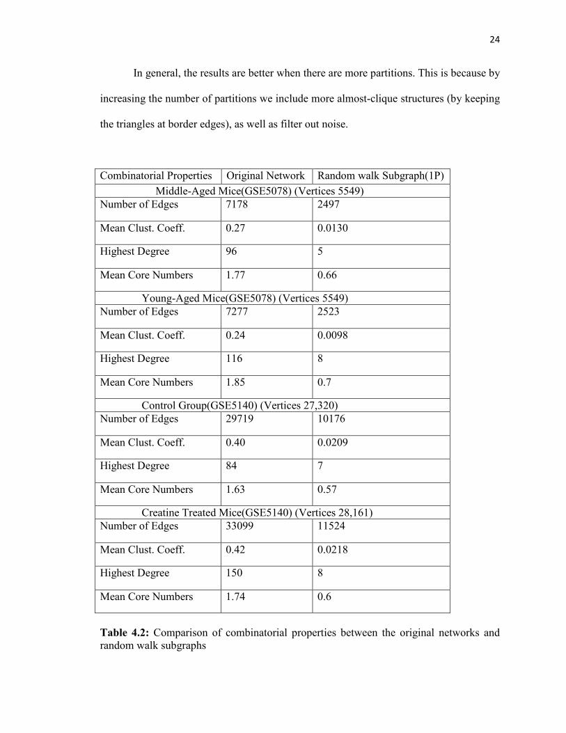
In general, the results are better when there are more partitions. This is because by

increasing the number of partitions we include more almost-clique structures (by keeping

the triangles at border edges), as well as filter out noise.

Combinatorial Properties Original Network Random walk Subgraph(1P) Middle-Aged Mice(GSE5078) (Vertices 5549) Number of Edges 7178 2497

Mean Clust. Coeff. 0.27 0.0130

Highest Degree 96 5

Mean Core Numbers 1.77 0.66

Young-Aged Mice(GSE5078) (Vertices 5549) Number of Edges 7277 2523

Mean Clust. Coeff. 0.24 0.0098

Highest Degree 116 8

Mean Core Numbers 1.85 0.7

Control Group(GSE5140) (Vertices 27,320) Number of Edges 29719 10176

Mean Clust. Coeff. 0.40 0.0209

Highest Degree 84 7

Mean Core Numbers 1.63 0.57

Creatine Treated Mice(GSE5140) (Vertices 28,161) Number of Edges 33099 11524

Mean Clust. Coeff. 0.42 0.0218

Highest Degree 150 8

Mean Core Numbers 1.74 0.6

Table 4.2: Comparison of combinatorial properties between the original networks and random walk subgraphs

25

From Table 4.2, we identified that random walk did not retain any combinatorial

properties and values are too low compared to chordal subgraph.

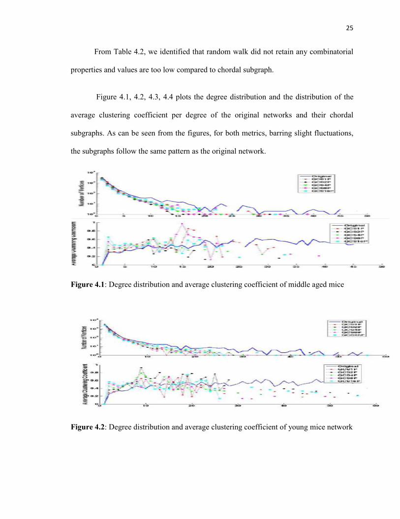
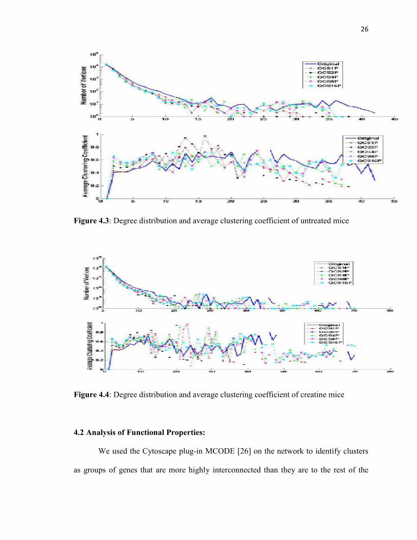
Figure 4.1, 4.2, 4.3, 4.4 plots the degree distribution and the distribution of the

average clustering coefficient per degree of the original networks and their chordal

subgraphs. As can be seen from the figures, for both metrics, barring slight fluctuations,

the subgraphs follow the same pattern as the original network.

Figure 4.1: Degree distribution and average clustering coefficient of middle aged mice

Figure 4.2: Degree distribution and average clustering coefficient of young mice network

26

Figure 4.3: Degree distribution and average clustering coefficient of untreated mice

Figure 4.4: Degree distribution and average clustering coefficient of creatine mice

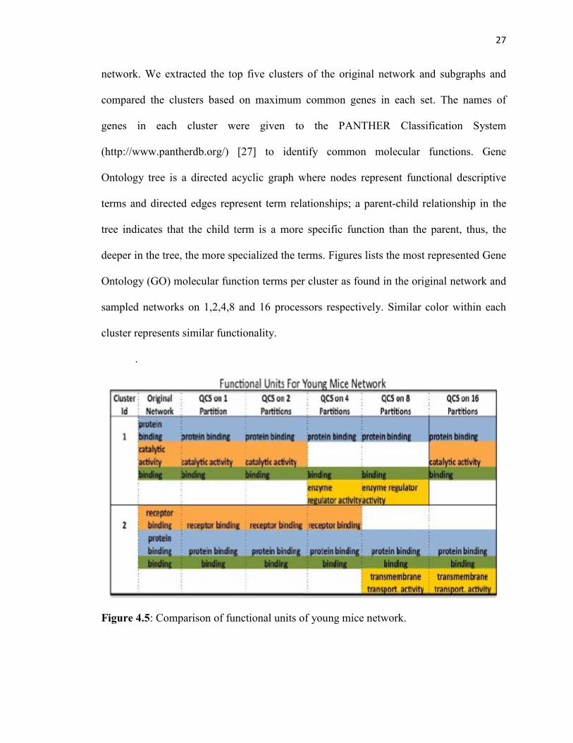
4.2 Analysis of Functional Properties:

We used the Cytoscape plug-in MCODE [26] on the network to identify clusters

as groups of genes that are more highly interconnected than they are to the rest of the

27

network. We extracted the top five clusters of the original network and subgraphs and

compared the clusters based on maximum common genes in each set. The names of

genes in each cluster were given to the PANTHER Classification System

(http://www.pantherdb.org/) [27] to identify common molecular functions. Gene

Ontology tree is a directed acyclic graph where nodes represent functional descriptive

terms and directed edges represent term relationships; a parent-child relationship in the

tree indicates that the child term is a more specific function than the parent, thus, the

deeper in the tree, the more specialized the terms. Figures lists the most represented Gene

Ontology (GO) molecular function terms per cluster as found in the original network and

sampled networks on 1,2,4,8 and 16 processors respectively. Similar color within each

cluster represents similar functionality.

.

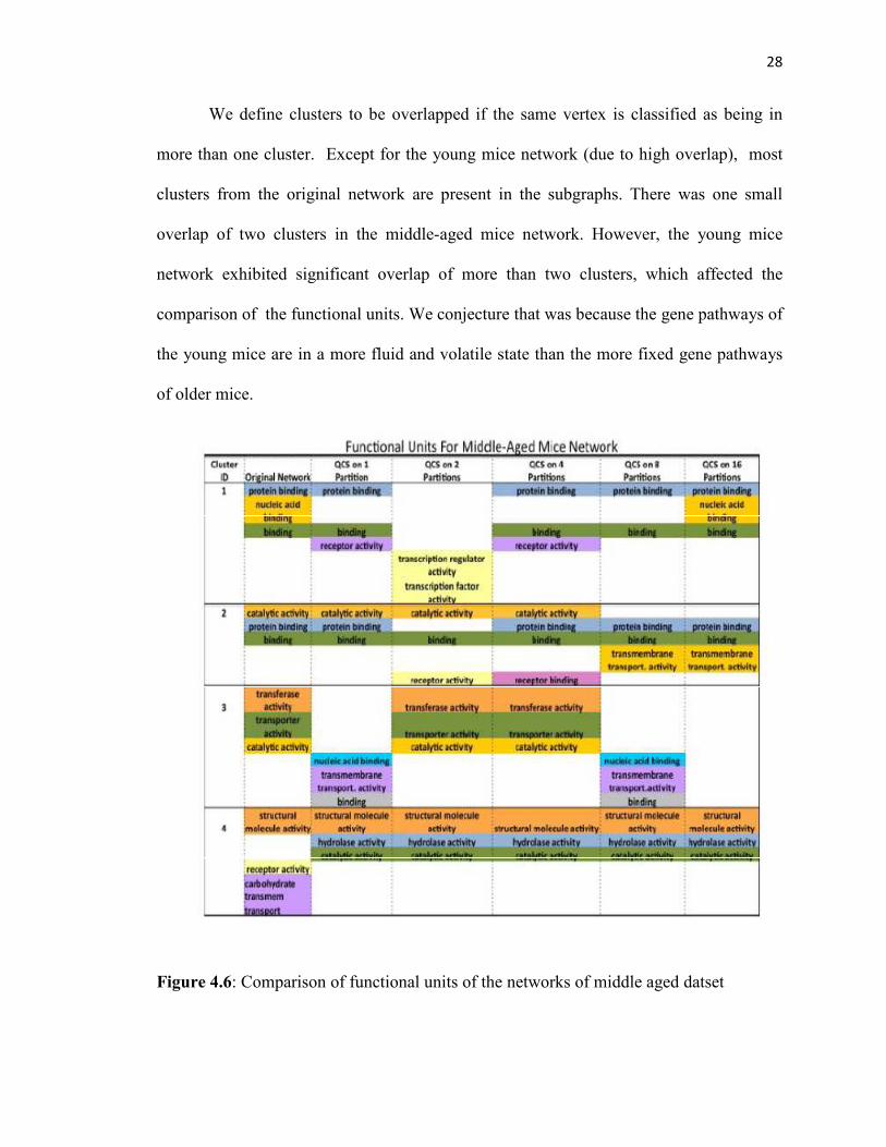
Figure 4.5: Comparison of functional units of young mice network.

28

We define clusters to be overlapped if the same vertex is classified as being in

more than one cluster. Except for the young mice network (due to high overlap), most

clusters from the original network are present in the subgraphs. There was one small

overlap of two clusters in the middle-aged mice network. However, the young mice

network exhibited significant overlap of more than two clusters, which affected the

comparison of the functional units. We conjecture that was because the gene pathways of

the young mice are in a more fluid and volatile state than the more fixed gene pathways

of older mice.

Figure 4.6: Comparison of functional units of the networks of middle aged datset

29

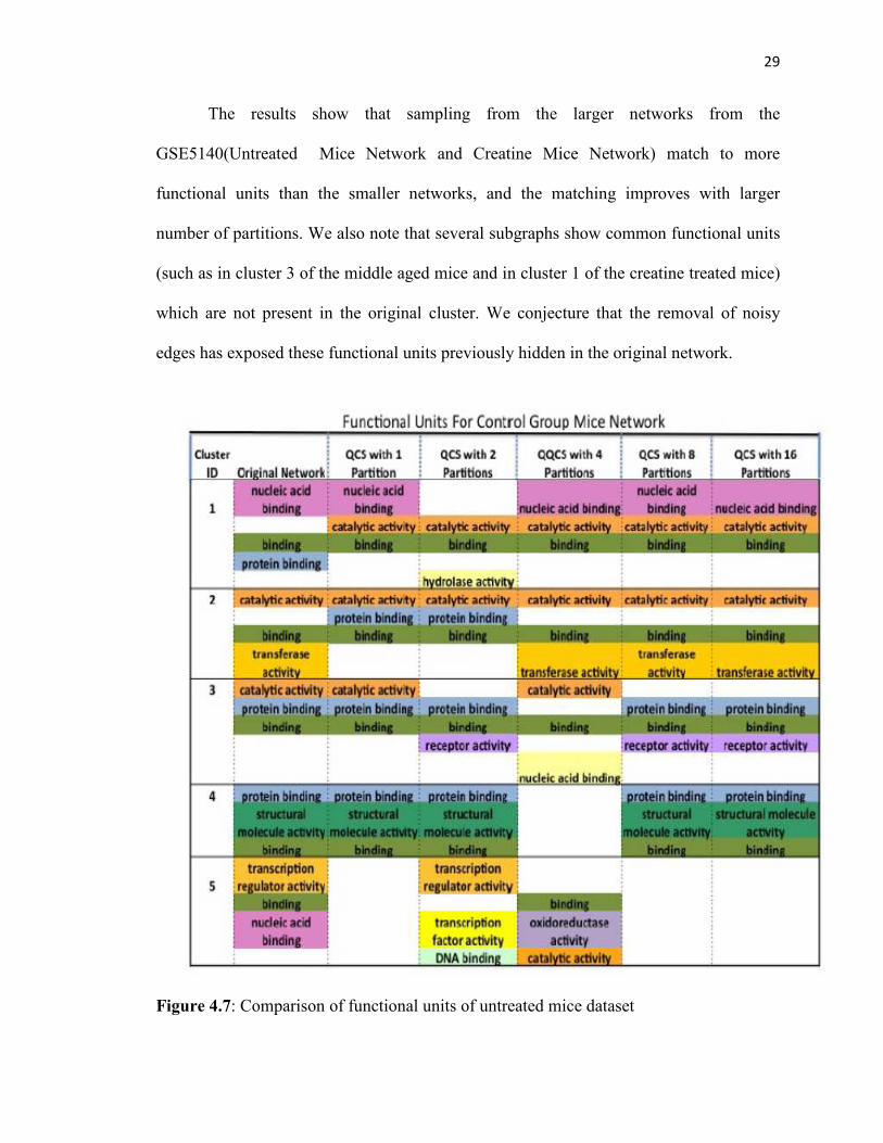
The results show that sampling from the larger networks from the

GSE5140(Untreated Mice Network and Creatine Mice Network) match to more

functional units than the smaller networks, and the matching improves with larger

number of partitions. We also note that several subgraphs show common functional units

(such as in cluster 3 of the middle aged mice and in cluster 1 of the creatine treated mice)

which are not present in the original cluster. We conjecture that the removal of noisy

edges has exposed these functional units previously hidden in the original network.

Figure 4.7: Comparison of functional units of untreated mice dataset

30

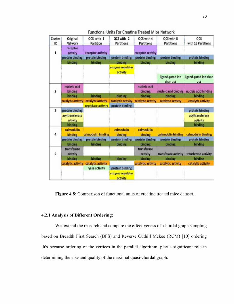
Figure 4.8: Comparison of functional units of creatine treated mice dataset.

4.2.1 Analysis of Different Ordering:

We extend the research and compare the effectiveness of chordal graph sampling

based on Breadth First Search (BFS) and Reverse Cuthill Mckee (RCM) [10] ordering

.It's because ordering of the vertices in the parallel algorithm, play a significant role in

determining the size and quality of the maximal quasi-chordal graph.

31

BFS ordering is based on a level by level traversal of the graph, where the level of

a vertex is its shortest distance from the starting vertex. BFS assures that the vertices in

the same connected graph component will be processed together.RCM ordering, in

addition to accessing connected components, ensures that closely connected groups of

vertices are placed together. RCM ordering is implemented by reversing the vertex order

obtained from a BFS search, with the constraint that the starting vertex is a peripheral

vertex [2].

Each column in the Figure 12 and 13 denotes clusters and corresponding

enrichment score found in the original network and through sampled networks on 1, 2, 4,

8, 16 and 32 processors respectively. Enrichment for a Gene Ontology term can be

described as the ratio of the number of genes in the cluster with the specified term (c) to

the number of genes in the cluster (n), divided by the ratio of the number of genes in the

entire genome with the specified term (C) to the total number of genes in the tested

genome (N). The formal equation to identify enrichment, then, is E = (c/n)/(C/N). The

higher the enrichment score, the better.

In the young mouse dataset, the original network had 2 of the top clusters

enriched in with GO terms associated with Development and Transport. Clusters

matching to these functionalities were also found in the sampling method using BFS

ordering (Figure 4.9). The BFS results identified the Development cluster (cluster 3) for

each number of partitions (1, 2, 4, 8, 16, and 32) whereas the Transport cluster (cluster 5)

was only identified on the sample using one processor. The BFS method also helped in

discovery of new clusters which were enriched in metabolism (cluster 1), development

(clusters 2 and 3), and transport (cluster 4).

32

In the case of RCM ordering (Figure 4.10), Metabolism enriched cluster (cluster

6) was preserved from the original network (for sampling in one processor and two

processors). New clusters identified were enriched in transport (cluster 2), metabolism

(cluster 1 and 3), and development (cluster 4). Compared to the BFS results (Figure 2),

these results were more functionally specific, suggesting that RCM may retain knowledge

better than BFS.

Figure 4.9: The gene functionality of clusters for the young mouse network with BFS ordering. Enrichment scores are colored from low (green) to high (red). Spaces with no enrichment means that for that number of partitions, there was no cluster found for that partition. Number of conserved clusters: 1. Number of clusters with additional genes: 1. Number of new clusters in sampled networks: 3.

33

Our results indicate that RCM had more matches to original GO clusters identified,

indicating that lowering the bandwidth of the corresponding matrix can help in obtaining

more clustered regions.

Figure 4.10: The gene functionality of clusters for the young mouse network with RCM ordering. Enrichment scores are colored from low (green) to high (red). Spaces with no enrichment means that for that number of partitions, there was no cluster found for that partition. Number of conserved clusters: 1. Number of new clusters in sampled networks: 6.

34

Additionally, both methods performed exceptionally at identifying novel clusters

within networks, which indicates that sampling based on identifying quasi chordal

subgraphs can indeed eliminate poorly connected edges, which form noise in the

network. RCM method had higher conservation of novel cluster identification than BFS

across number of partitions, suggesting that it may be more stable than the BFS method.

4.2.2 Analysis of Quality of Clusters:

Resulting cluster of both original network and sampled subgraphs are annotated

and scored and ranked according to true biological networks. All clusters from original

networks are compared to all clusters from sampled networks based on the following

metrics: (i) node overlap, (ii) edge overlap, (iii) biological relevance of clusters in the

original versus the sampled networks, (iv) number of known (found in the original

network) and new (not found in the original network) clusters identified.

We define some terms that is useful in understanding the subsequent explanation

of analysis of clusters.

Cluster Annotation and Scoring: For each edge e connecting nodes n1 and n2 in

some cluster C, the terms associated with genes represented by nodes n1 and n2 are

identified and mapped onto the GO biological process tree. Then the deepest common

parent/ancestor (DCP) of nodes n1 and n2 is identified and used to annotate edge e.

Scoring is performed using a measure of DCP depth (distance from the ROOT node to

the DCP) and term breadth ( length of the shortest path from term 1 and term 2) where

the final score of edge e is equal to DCP depth – term breadth[28]. Clusters are scored by

taking the average edge enrichment score (AEES) over all edges in the cluster and

35

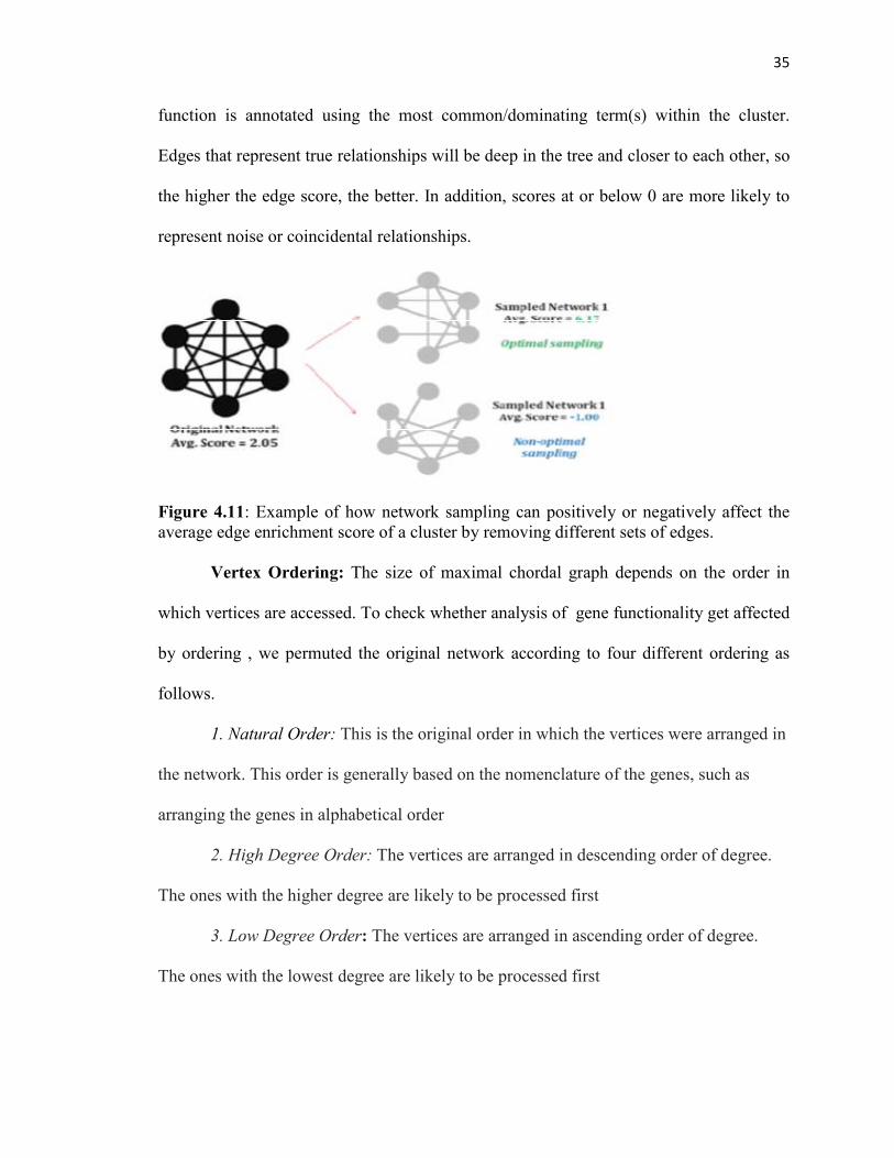
function is annotated using the most common/dominating term(s) within the cluster.

Edges that represent true relationships will be deep in the tree and closer to each other, so

the higher the edge score, the better. In addition, scores at or below 0 are more likely to

represent noise or coincidental relationships.

Figure 4.11: Example of how network sampling can positively or negatively affect the average edge enrichment score of a cluster by removing different sets of edges. Vertex Ordering: The size of maximal chordal graph depends on the order in

which vertices are accessed. To check whether analysis of gene functionality get affected

by ordering , we permuted the original network according to four different ordering as

follows.

1. Natural Order: This is the original order in which the vertices were arranged in

the network. This order is generally based on the nomenclature of the genes, such as

arranging the genes in alphabetical order

2. High Degree Order: The vertices are arranged in descending order of degree.

The ones with the higher degree are likely to be processed first

3. Low Degree Order: The vertices are arranged in ascending order of degree.

The ones with the lowest degree are likely to be processed first

36

4. Reverse Cut hill McKee (RCM Order): This ordering ensures that closely

connected group of vertices are placed together.

Cluster Overlap: We use the following measures to define sensitivity and specificity of

our filters as follows.

1. High AEES, High overlap (True Positive TP): Clusters that have a high AEES

and have a high (>50%) node or edge overlap indicates clusters that were found in the

original network and the sampled network, and the cluster has biological meaning.

2. Low AEES, High overlap (False Positive FP): Clusters that have a low AEES

and have a high (>50%) node or edge overlap indicates clusters that were found in the

original network and the sampled network, but the cluster likely has no biological

meaning.

3. High AEES, Low overlap (False Negative FN): Clusters that have a high AEES

and have a low (<50%) node or edge overlap indicates clusters that were not found in the

original network but were present in the sampled network, and have biological meaning.

These clusters tend to be small and less dense and are only uncovered when noise is

removed; hence they are hidden in the original network.

4. Low AEES, Low overlap (True Negative TN): Clusters that have a low AEES

and have a low (<50%) node or edge overlap indicates clusters that were not found in the

original network but were present in the sampled network, and likely have no biological

meaning.

By dividing the graph into equal quadrants, we can identify TP, FP, FN and TN

counts in figure 4.12.

37

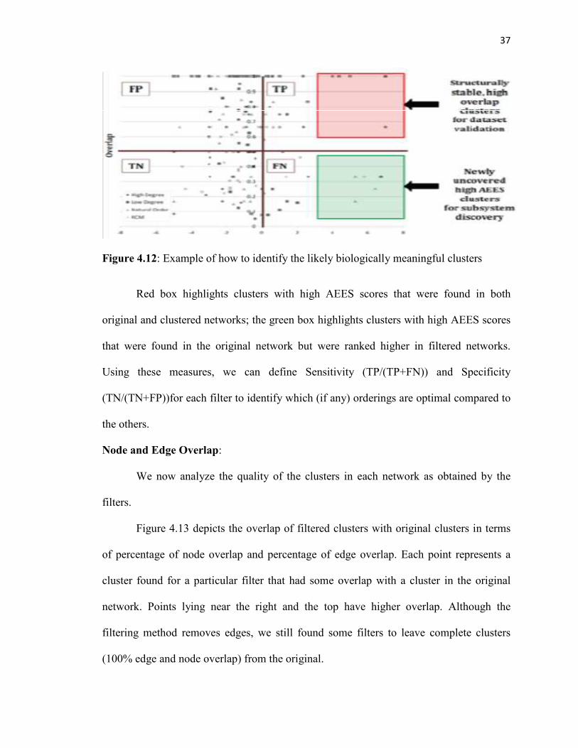
Figure 4.12: Example of how to identify the likely biologically meaningful clusters

Red box highlights clusters with high AEES scores that were found in both

original and clustered networks; the green box highlights clusters with high AEES scores

that were found in the original network but were ranked higher in filtered networks.

Using these measures, we can define Sensitivity (TP/(TP+FN)) and Specificity

(TN/(TN+FP))for each filter to identify which (if any) orderings are optimal compared to

the others.

Node and Edge Overlap:

We now analyze the quality of the clusters in each network as obtained by the

filters.

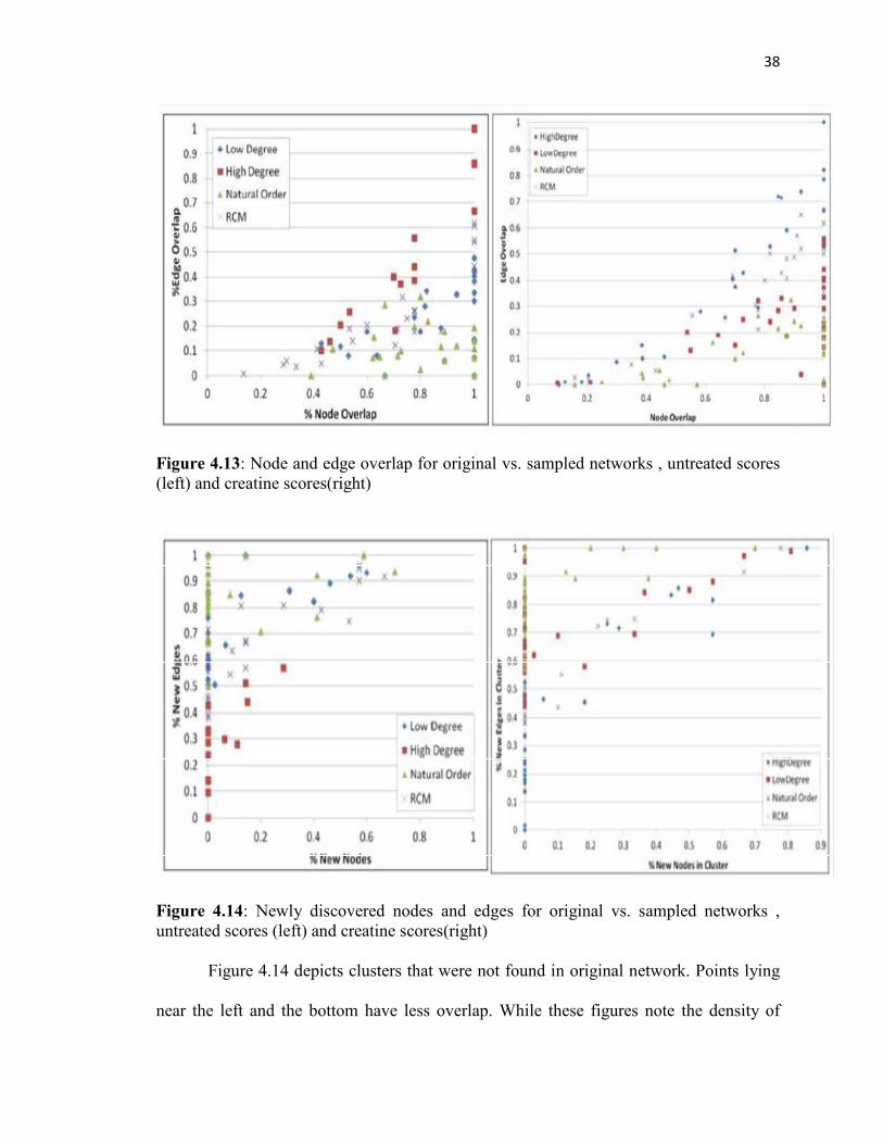
Figure 4.13 depicts the overlap of filtered clusters with original clusters in terms

of percentage of node overlap and percentage of edge overlap. Each point represents a

cluster found for a particular filter that had some overlap with a cluster in the original

network. Points lying near the right and the top have higher overlap. Although the

filtering method removes edges, we still found some filters to leave complete clusters

(100% edge and node overlap) from the original.

38

Figure 4.13: Node and edge overlap for original vs. sampled networks , untreated scores (left) and creatine scores(right)

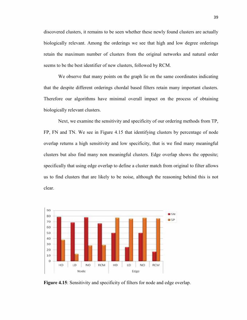
Figure 4.14: Newly discovered nodes and edges for original vs. sampled networks , untreated scores (left) and creatine scores(right)

Figure 4.14 depicts clusters that were not found in original network. Points lying

near the left and the bottom have less overlap. While these figures note the density of

39

discovered clusters, it remains to be seen whether these newly found clusters are actually

biologically relevant. Among the orderings we see that high and low degree orderings

retain the maximum number of clusters from the original networks and natural order

seems to be the best identifier of new clusters, followed by RCM.

We observe that many points on the graph lie on the same coordinates indicating

that the despite different orderings chordal based filters retain many important clusters.

Therefore our algorithms have minimal overall impact on the process of obtaining

biologically relevant clusters.

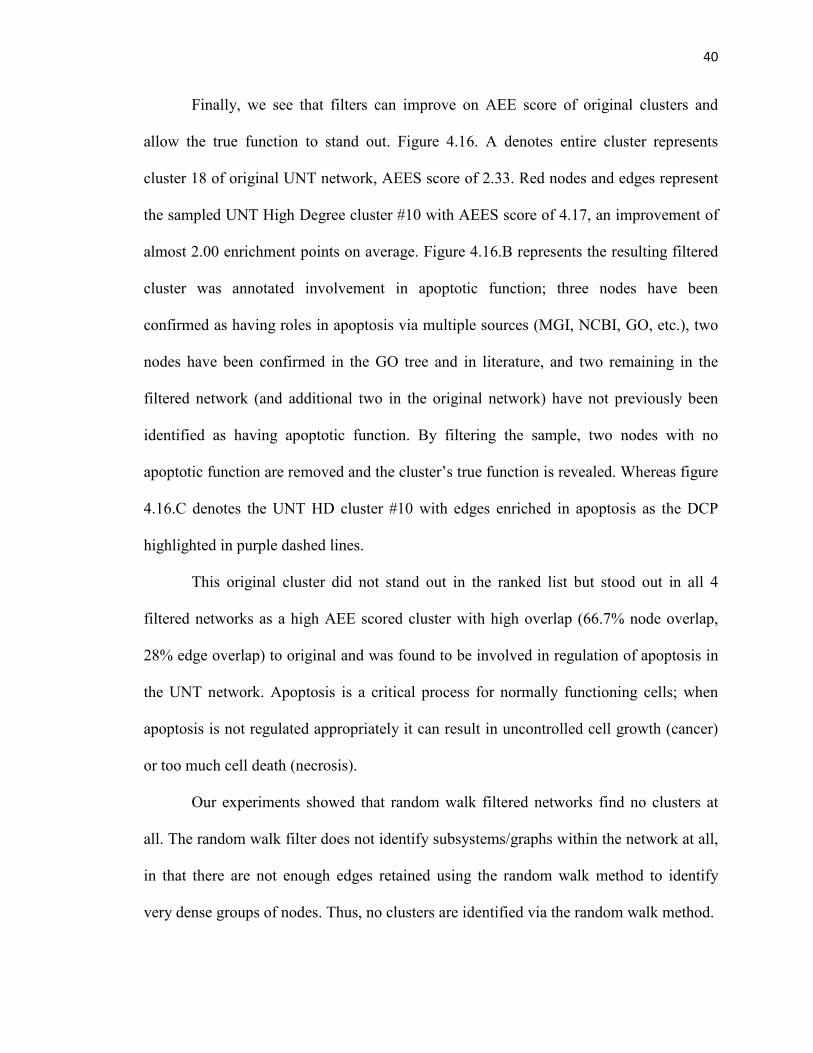
Next, we examine the sensitivity and specificity of our ordering methods from TP,

FP, FN and TN. We see in Figure 4.15 that identifying clusters by percentage of node

overlap returns a high sensitivity and low specificity, that is we find many meaningful

clusters but also find many non meaningful clusters. Edge overlap shows the opposite;

specifically that using edge overlap to define a cluster match from original to filter allows

us to find clusters that are likely to be noise, although the reasoning behind this is not

clear.

Figure 4.15: Sensitivity and specificity of filters for node and edge overlap.

40

Finally, we see that filters can improve on AEE score of original clusters and

allow the true function to stand out. Figure 4.16. A denotes entire cluster represents

cluster 18 of original UNT network, AEES score of 2.33. Red nodes and edges represent

the sampled UNT High Degree cluster #10 with AEES score of 4.17, an improvement of

almost 2.00 enrichment points on average. Figure 4.16.B represents the resulting filtered

cluster was annotated involvement in apoptotic function; three nodes have been

confirmed as having roles in apoptosis via multiple sources (MGI, NCBI, GO, etc.), two

nodes have been confirmed in the GO tree and in literature, and two remaining in the

filtered network (and additional two in the original network) have not previously been

identified as having apoptotic function. By filtering the sample, two nodes with no

apoptotic function are removed and the cluster’s true function is revealed. Whereas figure

4.16.C denotes the UNT HD cluster #10 with edges enriched in apoptosis as the DCP

highlighted in purple dashed lines.

This original cluster did not stand out in the ranked list but stood out in all 4

filtered networks as a high AEE scored cluster with high overlap (66.7% node overlap,

28% edge overlap) to original and was found to be involved in regulation of apoptosis in

the UNT network. Apoptosis is a critical process for normally functioning cells; when

apoptosis is not regulated appropriately it can result in uncontrolled cell growth (cancer)

or too much cell death (necrosis).

Our experiments showed that random walk filtered networks find no clusters at

all. The random walk filter does not identify subsystems/graphs within the network at all,

in that there are not enough edges retained using the random walk method to identify

very dense groups of nodes. Thus, no clusters are identified via the random walk method.

41

Figure 4.16: Example of how filtering impacts a cluster.

4.3 Analysis of Parallel Results:

We demonstrate the scalability of our parallel chordal graph based sampling

algorithm. Our experiments were performed on the Firefly Cluster at the Holland

Computing Center. Firefly is a Linux-based system comprising of AMD quad- and dual-

core processors. Our implementation was based on a distributed memory approach using

MPI. We compared the scalability of the following three sampling algorithms: (i) chordal

42

graph based sampling using communication, (ii) chordal graph based sampling without

communication, and (iii) random walk.

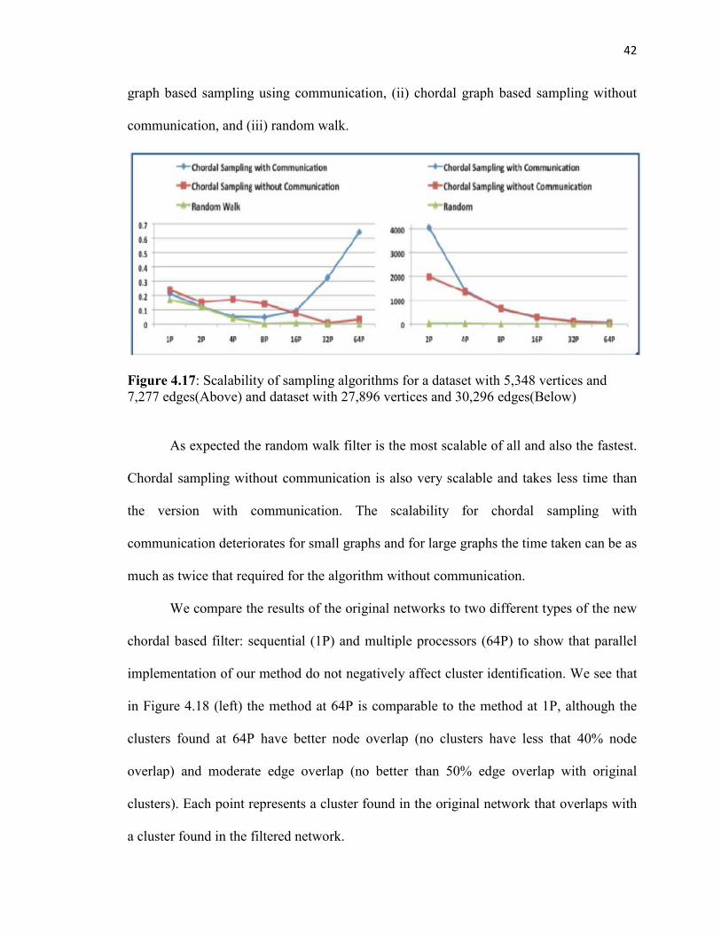
Figure 4.17: Scalability of sampling algorithms for a dataset with 5,348 vertices and 7,277 edges(Above) and dataset with 27,896 vertices and 30,296 edges(Below)

As expected the random walk filter is the most scalable of all and also the fastest.

Chordal sampling without communication is also very scalable and takes less time than

the version with communication. The scalability for chordal sampling with

communication deteriorates for small graphs and for large graphs the time taken can be as

much as twice that required for the algorithm without communication.

We compare the results of the original networks to two different types of the new

chordal based filter: sequential (1P) and multiple processors (64P) to show that parallel

implementation of our method do not negatively affect cluster identification. We see that

in Figure 4.18 (left) the method at 64P is comparable to the method at 1P, although the

clusters found at 64P have better node overlap (no clusters have less that 40% node

overlap) and moderate edge overlap (no better than 50% edge overlap with original

clusters). Each point represents a cluster found in the original network that overlaps with

a cluster found in the filtered network.

43

Figure 4.18: Parallel results for Creatine Natural Order filter.

Figure 4.18(Right) represents Clusters with AEES scores >3.0 found in original,

1P and 64P networks. The average depth is the AEES score, and Max Score represents

the deepest term represented in the cluster.

44

Chapter 5

Conclusion

We developed and implemented a scalable parallel graph sampling algorithms

based on extracting the maximal chordal subgraphs from large networks. We showed that

our sampled subgraphs retain most of the combinatorial and functional properties of the

original network. We present the detailed analysis of clusters obtained by comparing the

random filter method and also chordal graph with different permutations of network. Our

analysis show that maximal chordal subgraphs will maintain or improve upon the

biological information contained within the highly dense subgraphs. Reported results also

show that our parallel implementation is scalable and the analysis results are not

significantly affected by data distribution and ordering of vertices. Thus, our method tries

to find the best description of the network being analyzed, no matter what kind of

network.

As a part of future work, we can investigate the impact of implementing other

methods for reducing noise in the network, such as identifying Steiner trees or

Hypergraph and also continue the network sampling on weighted networks and on

dynamic evolving networks.

45

References:

[1] J. C. Miller and J. M. Hyman. Effective vaccination strategies for realistic social

networks. Physica A.386,780-785(2007).

[2] K. Voevodski, S. H. Teng, and Y. Xia. Finding local communities in protein networks

BMC Bioinformatics,10, 297(2009).

[3] R. Yokomori, H. Siy, M. Noro, and K. Inoue. Assessing the Impact of Framework

Changes Using Component Ranking. International Conference on Software Maintenance.

ICSM '09.2009.

[4] D. A. Bader, G. Cong. A Fast, Parallel Spanning Tree Algorithm for Symmetric

Multiprocessors.18th International Parallel and Distributed Processing Symposium.

IPDPS'04.

[5] G. Cong, G. Almasi, V. Saraswat. A Fast PGAS Implementation of Distributed Graph

Algorithms. Proceedings of the 2010 ACM/IEEE International Conference for High

Performance Computing, Networking, Storage and Analysis, SC’10. 2010.

[6] V. Agarwal, F. Petrini, D. Pasetto and D. A. Bader. Scalable Graph Exploration on

Multicore Processors. Proceedings of the 2010 ACM/IEEE International Conference for

High Performance Computing, Networking, Storage and Analysis. SC’10. 2010.

[7] J. Leskovec and C. Faloutsos. Sampling from large graphs. Proceedings of the 12th

ACM SIGKDD international conference on Knowledge discovery and data mining,

KDD’06. 2006.

[8] V. Krishnamurthy, M. Faloutsos, J.-H. Chrobak, M. Cui, L. Lao, and A. G. Percus.

Sampling large internet topologies for simulation purposes. Computer Networks 51,

2007, 4284–4302.

46

[9] J. Leskovec, J. Kleinberg, C. Faloutsos. Graphs over time: densification laws,

shrinking diameters and possible explanations. Proceedings of the eleventh ACM

SIGKDD international conference on Knowledge discovery in data mining, KDD’05.

2005.

[10] J. L. Gross, J. Yellen. Handbook of Graph Theory and Applications, CRC Press,

2004.

[11] D.rafiei ,s.curial ,Effectively Visualizing Large Networks Through Sampling, In

Visualization,2005

[12] A.Gilbert, K. Levchenko ,Compressing Network Graphs, In LinkKDD,2004

[13] Mashaghi.A et al, Investigation of a Protein Complex Network, European Physical

Journal,B41(1):113-121

[14]Arun.S.Maiya and Tanya.Y.Berger Wolf. Benefits of Bias: Towards better

Characterization of network sampling.Proceedings of KDD'11.2011

[15] A. Rasti, M. Torkjazi, R. Rejaie, N. Duffield, W. Willinger, D. Stutzbach,

Respondent-driven sampling for characterizing unstructured overlays, INFOCOM 2009.

pp. 2701–2705.

[16] A. Miranda, L. Garcia, A. Carvalho, and A. Lorena, Use of classification algorithms

in noise detection and elimination. Hybrid Artificial Intelligence Systems, Lecture Notes

in Computer Science, 5572. 2009, pp. 417–424.

47

[17] G. L. Libralon, A. Carvalho, and A. C. Lorena, Preprocessing for noise detection in

gene expression classification data. Journal of the Brazilian Computer Society 15.2009, 3

–11.

[18] P. M. Dearing, D. R. Shier and D. D. Warner, Maximal Chordal Subgraphs, Discrete

Applied Mathematics.20, 3,1988. 181-190.

[19] N. S. Watson-Haigh, H. N. Kadarmideen, A. Reverter, Pcit: An r package for

weighted gene co-expression networks based on partial correlation and information

theory approaches, Bioinformatics(Oxford, England) 26 (3) (2010) 411–413.

[20] W. J. Ewens, G. R. Grant, Statistical methods in bioinformatics (Second Edition

ed.), New York, NY: Springer, 2005.

[21] M. Mutwil, U. B., S. M., A. Loraine, O. Ebenhoh, S. Persson, Assembly of an

interactive correlation network for the arabidopsis genome using a novel heuristic

clustering algorithm, Plant Physiology 152 (1) (2010) 29–43.

[22] A. L. Barabasi, Z. N. Oltvai, Network biology: Understanding the cell’s functional

organization, Nature Reviews.Genetics 5 (2) (2004) 101–113.

[23] Verbitsky, M, Yonan, AL, Malleret, G, Kandel, ER, Gilliam, T C, & Pavlidis, P.

(2004). Altered hippocampal transcript profile accompanies an age-related spatial

memory deficit in mice. Learning & Memory (Cold Spring Harbor, N.Y.), 11(3), 253-

260.

[24] Bender A, Beckers J, Schneider I, Hölter SM et al. Creatine improves health and

survival of mice. Neurobiol Aging 2008 Sep;29(9):1404-11. PMID: 17416441.

[25] MatlabBGL Library(http://www.stanford.edu/dgleich/programs/matlab bgl/).

48

[26] G. D. Bader, C.W. Hogue, An automated method for finding molecular complexes

in large protein interaction networks, BMC Bioinformatics 4 (2).

[27] P. Thomas, M. J. Canpbell, A. Kejariwal, M. Huaiyu, B. Karlak, R. Daverman, K.

Diemer, A. Muruganujan, N. A., Panther: a library of protein families and subfamilies

indexed by function, Genome Res. 13 (2003) 2129–2141.

[28] Dempsey, K, Thapa, I, Bastola, D, and Ali, H. (2011) Identifying Modular Function

via Edge Annotation in Gene Correlation Networks using Gene Ontology Search. 2011

BIBM Workshop on Data Mining for Biomarker Discovery: November 2011. Atlanta,

GA

[29] A.Barabasi ,R.Alber ,”Emergence of scaling in random networks”,1999

[30] K. Dempsey, K. Duraisamy, H. Ali, S. Bhowmick, A parallel graph sampling

algorithm for analyzing gene correlation networks. International Conference in

Computational Science 2011. ICCS’11. 2011.

[31] K. Duraisamy, K.Dempsey, H. Ali, S. Bhowmick, A noise reducing sampling

approach for uncovering critical properties in large scale biological networks. The 2011

International Conference on High Performance Computing & Simulation. HPCS’11.

[32] K.Dempsey, K.Duraisamy, S.Bhowmick, H.Ali, The Developement of Parallel

Adaptive Sampling Algorithms for Analyzing Biological Networks . The 2012

International Workshop on High Performance Computational Biology.HICOMB'12.

[33] Y. Saad, “Iterative Methods for Sparse Linear Systems”, PWS Publishing Company,

1995