Paradis BeginnersR En
76
R for Beginners Emmanuel Paradis Institut des Sciences de l’ ´ Evolution Universit´ e Montpellier II F-34095 Montpellier c´ edex 05 France E-mail: [email protected]
description
R-statistics
Transcript of Paradis BeginnersR En

R for Beginners
Emmanuel Paradis
Institut des Sciences de l’EvolutionUniversite Montpellier II
F-34095 Montpellier cedex 05France
E-mail: [email protected]

I thank Julien Claude, Christophe Declercq, Elodie Gazave, Friedrich Leisch,Louis Luangkesron, Francois Pinard, and Mathieu Ros for their comments andsuggestions on earlier versions of this document. I am also grateful to all themembers of the R Development Core Team for their considerable efforts indeveloping R and animating the discussion list ‘rhelp’. Thanks also to theR users whose questions or comments helped me to write “R for Beginners”.Special thanks to Jorge Ahumada for the Spanish translation.
c© 2002, 2005, Emmanuel Paradis (12th September 2005)
Permission is granted to make and distribute copies, either in part or infull and in any language, of this document on any support provided the abovecopyright notice is included in all copies. Permission is granted to translatethis document, either in part or in full, in any language provided the abovecopyright notice is included.

Contents
1 Preamble 1
2 A few concepts before starting 32.1 How R works . . . . . . . . . . . . . . . . . . . . . . . . . . . . 32.2 Creating, listing and deleting the objects in memory . . . . . . 52.3 The on-line help . . . . . . . . . . . . . . . . . . . . . . . . . . 7
3 Data with R 93.1 Objects . . . . . . . . . . . . . . . . . . . . . . . . . . . . . . . 93.2 Reading data in a file . . . . . . . . . . . . . . . . . . . . . . . 113.3 Saving data . . . . . . . . . . . . . . . . . . . . . . . . . . . . . 143.4 Generating data . . . . . . . . . . . . . . . . . . . . . . . . . . 15
3.4.1 Regular sequences . . . . . . . . . . . . . . . . . . . . . 153.4.2 Random sequences . . . . . . . . . . . . . . . . . . . . . 17
3.5 Manipulating objects . . . . . . . . . . . . . . . . . . . . . . . . 183.5.1 Creating objects . . . . . . . . . . . . . . . . . . . . . . 183.5.2 Converting objects . . . . . . . . . . . . . . . . . . . . . 233.5.3 Operators . . . . . . . . . . . . . . . . . . . . . . . . . . 253.5.4 Accessing the values of an object: the indexing system . 263.5.5 Accessing the values of an object with names . . . . . . 293.5.6 The data editor . . . . . . . . . . . . . . . . . . . . . . . 313.5.7 Arithmetics and simple functions . . . . . . . . . . . . . 313.5.8 Matrix computation . . . . . . . . . . . . . . . . . . . . 33
4 Graphics with R 364.1 Managing graphics . . . . . . . . . . . . . . . . . . . . . . . . . 36
4.1.1 Opening several graphical devices . . . . . . . . . . . . . 364.1.2 Partitioning a graphic . . . . . . . . . . . . . . . . . . . 37
4.2 Graphical functions . . . . . . . . . . . . . . . . . . . . . . . . . 404.3 Low-level plotting commands . . . . . . . . . . . . . . . . . . . 414.4 Graphical parameters . . . . . . . . . . . . . . . . . . . . . . . 434.5 A practical example . . . . . . . . . . . . . . . . . . . . . . . . 444.6 The grid and lattice packages . . . . . . . . . . . . . . . . . . . 48
5 Statistical analyses with R 555.1 A simple example of analysis of variance . . . . . . . . . . . . . 555.2 Formulae . . . . . . . . . . . . . . . . . . . . . . . . . . . . . . 565.3 Generic functions . . . . . . . . . . . . . . . . . . . . . . . . . . 585.4 Packages . . . . . . . . . . . . . . . . . . . . . . . . . . . . . . . 61

6 Programming with R in pratice 646.1 Loops and vectorization . . . . . . . . . . . . . . . . . . . . . . 646.2 Writing a program in R . . . . . . . . . . . . . . . . . . . . . . 666.3 Writing your own functions . . . . . . . . . . . . . . . . . . . . 67
7 Literature on R 71

1 Preamble
The goal of the present document is to give a starting point for people newlyinterested in R. I chose to emphasize on the understanding of how R works,with the aim of a beginner, rather than expert, use. Given that the possibilitiesoffered by R are vast, it is useful to a beginner to get some notions andconcepts in order to progress easily. I tried to simplify the explanations asmuch as I could to make them understandable by all, while giving usefuldetails, sometimes with tables.
R is a system for statistical analyses and graphics created by Ross Ihakaand Robert Gentleman1. R is both a software and a language considered as adialect of the S language created by the AT&T Bell Laboratories. S is availableas the software S-PLUS commercialized by Insightful2. There are importantdifferences in the designs of R and of S: those who want to know more on thispoint can read the paper by Ihaka & Gentleman (1996) or the R-FAQ3, a copyof which is also distributed with R.
R is freely distributed under the terms of the GNU General Public Licence4;its development and distribution are carried out by several statisticians knownas the R Development Core Team.
R is available in several forms: the sources (written mainly in C andsome routines in Fortran), essentially for Unix and Linux machines, or somepre-compiled binaries for Windows, Linux, and Macintosh. The files neededto install R, either from the sources or from the pre-compiled binaries, aredistributed from the internet site of the Comprehensive R Archive Network(CRAN)5 where the instructions for the installation are also available. Re-garding the distributions of Linux (Debian, . . . ), the binaries are generallyavailable for the most recent versions; look at the CRAN site if necessary.
R has many functions for statistical analyses and graphics; the latter arevisualized immediately in their own window and can be saved in various for-mats (jpg, png, bmp, ps, pdf, emf, pictex, xfig; the available formats maydepend on the operating system). The results from a statistical analysis aredisplayed on the screen, some intermediate results (P-values, regression coef-ficients, residuals, . . . ) can be saved, written in a file, or used in subsequentanalyses.
The R language allows the user, for instance, to program loops to suc-cessively analyse several data sets. It is also possible to combine in a singleprogram different statistical functions to perform more complex analyses. The
1Ihaka R. & Gentleman R. 1996. R: a language for data analysis and graphics. Journal
of Computational and Graphical Statistics 5: 299–314.2See http://www.insightful.com/products/splus/default.asp for more information3http://cran.r-project.org/doc/FAQ/R-FAQ.html4For more information: http://www.gnu.org/5http://cran.r-project.org/
1

R users may benefit from a large number of programs written for S and avail-able on the internet6, most of these programs can be used directly with R.
At first, R could seem too complex for a non-specialist. This may notbe true actually. In fact, a prominent feature of R is its flexibility. Whereasa classical software displays immediately the results of an analysis, R storesthese results in an “object”, so that an analysis can be done with no resultdisplayed. The user may be surprised by this, but such a feature is very useful.Indeed, the user can extract only the part of the results which is of interest.For example, if one runs a series of 20 regressions and wants to compare thedifferent regression coefficients, R can display only the estimated coefficients:thus the results may take a single line, whereas a classical software could wellopen 20 results windows. We will see other examples illustrating the flexibilityof a system such as R compared to traditional softwares.
6For example: http://stat.cmu.edu/S/
2

2 A few concepts before starting
Once R is installed on your computer, the software is executed by launchingthe corresponding executable. The prompt, by default ‘>’, indicates that Ris waiting for your commands. Under Windows using the program Rgui.exe,some commands (accessing the on-line help, opening files, . . . ) can be executedvia the pull-down menus. At this stage, a new user is likely to wonder “Whatdo I do now?” It is indeed very useful to have a few ideas on how R workswhen it is used for the first time, and this is what we will see now.
We shall see first briefly how R works. Then, I will describe the “assign”operator which allows creating objects, how to manage objects in memory,and finally how to use the on-line help which is very useful when running R.
2.1 How R works
The fact that R is a language may deter some users who think “I can’t pro-gram”. This should not be the case for two reasons. First, R is an interpretedlanguage, not a compiled one, meaning that all commands typed on the key-board are directly executed without requiring to build a complete programlike in most computer languages (C, Fortran, Pascal, . . . ).
Second, R’s syntax is very simple and intuitive. For instance, a linearregression can be done with the command lm(y ~ x) which means “fittinga linear model with y as response and x as predictor”. In R, in order tobe executed, a function always needs to be written with parentheses, evenif there is nothing within them (e.g., ls()). If one just types the name of afunction without parentheses, R will display the content of the function. In thisdocument, the names of the functions are generally written with parentheses inorder to distinguish them from other objects, unless the text indicates clearlyso.
When R is running, variables, data, functions, results, etc, are stored inthe active memory of the computer in the form of objects which have a name.The user can do actions on these objects with operators (arithmetic, logical,comparison, . . . ) and functions (which are themselves objects). The use ofoperators is relatively intuitive, we will see the details later (p. 25). An Rfunction may be sketched as follows:
arguments −→
options −→
function
↑default arguments
=⇒result
The arguments can be objects (“data”, formulae, expressions, . . . ), some
3

of which could be defined by default in the function; these default values maybe modified by the user by specifying options. An R function may require noargument: either all arguments are defined by default (and their values can bemodified with the options), or no argument has been defined in the function.We will see later in more details how to use and build functions (p. 67). Thepresent description is sufficient for the moment to understand how R works.
All the actions of R are done on objects stored in the active memory ofthe computer: no temporary files are used (Fig. 1). The readings and writingsof files are used for input and output of data and results (graphics, . . . ). Theuser executes the functions via some commands. The results are displayeddirectly on the screen, stored in an object, or written on the disk (particularlyfor graphics). Since the results are themselves objects, they can be consideredas data and analysed as such. Data files can be read from the local disk orfrom a remote server through internet.
functions and operators
?
“data” objects
?6
����)XXXXXXXz
“results” objects
.../library/base/
/stast/
/graphics/
...
library offunctions
�
datafiles
� -
internet�
PS JPEG . . .
keyboardmouse
-commands
screen
Active memory Hard disk
Figure 1: A schematic view of how R works.
The functions available to the user are stored in a library localised onthe disk in a directory called R HOME/library (R HOME is the directorywhere R is installed). This directory contains packages of functions, which arethemselves structured in directories. The package named base is in a way thecore of R and contains the basic functions of the language, particularly, forreading and manipulating data. Each package has a directory called R witha file named like the package (for instance, for the package base, this is thefile R HOME/library/base/R/base). This file contains all the functions of thepackage.
One of the simplest commands is to type the name of an object to displayits content. For instance, if an object n contents the value 10:
> n
[1] 10
4

The digit 1 within brackets indicates that the display starts at the firstelement of n. This command is an implicit use of the function print and theabove example is similar to print(n) (in some situations, the function print
must be used explicitly, such as within a function or a loop).The name of an object must start with a letter (A–Z and a–z) and can
include letters, digits (0–9), dots (.), and underscores ( ). R discriminatesbetween uppercase letters and lowercase ones in the names of the objects, sothat x and X can name two distinct objects (even under Windows).
2.2 Creating, listing and deleting the objects in memory
An object can be created with the “assign” operator which is written as anarrow with a minus sign and a bracket; this symbol can be oriented left-to-rightor the reverse:
> n <- 15
> n
[1] 15
> 5 -> n
> n
[1] 5
> x <- 1
> X <- 10
> x
[1] 1
> X
[1] 10
If the object already exists, its previous value is erased (the modificationaffects only the objects in the active memory, not the data on the disk). Thevalue assigned this way may be the result of an operation and/or a function:
> n <- 10 + 2
> n
[1] 12
> n <- 3 + rnorm(1)
> n
[1] 2.208807
The function rnorm(1) generates a normal random variate with mean zeroand variance unity (p. 17). Note that you can simply type an expressionwithout assigning its value to an object, the result is thus displayed on thescreen but is not stored in memory:
> (10 + 2) * 5
[1] 60
5

The assignment will be omitted in the examples if not necessary for un-derstanding.
The function ls lists simply the objects in memory: only the names of theobjects are displayed.
> name <- "Carmen"; n1 <- 10; n2 <- 100; m <- 0.5
> ls()
[1] "m" "n1" "n2" "name"
Note the use of the semi-colon to separate distinct commands on the sameline. If we want to list only the objects which contain a given character intheir name, the option pattern (which can be abbreviated with pat) can beused:
> ls(pat = "m")
[1] "m" "name"
To restrict the list of objects whose names start with this character:
> ls(pat = "^m")
[1] "m"
The function ls.str displays some details on the objects in memory:
> ls.str()
m : num 0.5
n1 : num 10
n2 : num 100
name : chr "Carmen"
The option pattern can be used in the same way as with ls. Anotheruseful option of ls.str is max.level which specifies the level of detail for thedisplay of composite objects. By default, ls.str displays the details of allobjects in memory, included the columns of data frames, matrices and lists,which can result in a very long display. We can avoid to display all thesedetails with the option max.level = -1:
> M <- data.frame(n1, n2, m)
> ls.str(pat = "M")
M : ‘data.frame’: 1 obs. of 3 variables:
$ n1: num 10
$ n2: num 100
$ m : num 0.5
> ls.str(pat="M", max.level=-1)
M : ‘data.frame’: 1 obs. of 3 variables:
To delete objects in memory, we use the function rm: rm(x) deletes theobject x, rm(x,y) deletes both the objects x et y, rm(list=ls()) deletes allthe objects in memory; the same options mentioned for the function ls() canthen be used to delete selectively some objects: rm(list=ls(pat="^m")).
6

2.3 The on-line help
The on-line help of R gives very useful information on how to use the functions.Help is available directly for a given function, for instance:
> ?lm
will display, within R, the help page for the function lm() (linear model). Thecommands help(lm) and help("lm") have the same effect. The last one mustbe used to access help with non-conventional characters:
> ?*
Error: syntax error
> help("*")
Arithmetic package:base R Documentation
Arithmetic Operators
...
Calling help opens a page (this depends on the operating system) withgeneral information on the first line such as the name of the package whereis (are) the documented function(s) or operators. Then comes a title followedby sections which give detailed information.
Description: brief description.
Usage: for a function, gives the name with all its arguments and the possibleoptions (with the corresponding default values); for an operator givesthe typical use.
Arguments: for a function, details each of its arguments.
Details: detailed description.
Value: if applicable, the type of object returned by the function or the oper-ator.
See Also: other help pages close or similar to the present one.
Examples: some examples which can generally be executed without openingthe help with the function example.
For beginners, it is good to look at the section Examples. Generally, itis useful to read carefully the section Arguments. Other sections may beencountered, such as Note, References or Author(s).
By default, the function help only searches in the packages which areloaded in memory. The option try.all.packages, which default is FALSE,allows to search in all packages if its value is TRUE:
7
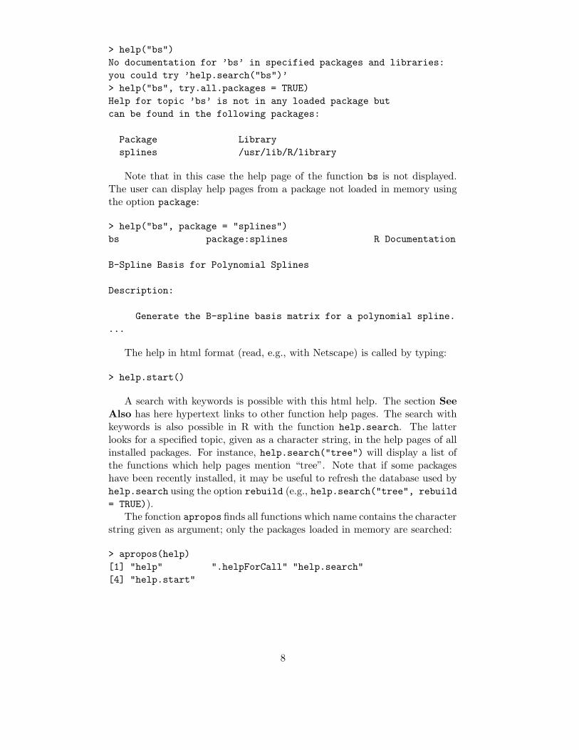
> help("bs")
No documentation for ’bs’ in specified packages and libraries:
you could try ’help.search("bs")’
> help("bs", try.all.packages = TRUE)
Help for topic ’bs’ is not in any loaded package but
can be found in the following packages:
Package Library
splines /usr/lib/R/library
Note that in this case the help page of the function bs is not displayed.The user can display help pages from a package not loaded in memory usingthe option package:
> help("bs", package = "splines")
bs package:splines R Documentation
B-Spline Basis for Polynomial Splines
Description:
Generate the B-spline basis matrix for a polynomial spline.
...
The help in html format (read, e.g., with Netscape) is called by typing:
> help.start()
A search with keywords is possible with this html help. The section SeeAlso has here hypertext links to other function help pages. The search withkeywords is also possible in R with the function help.search. The latterlooks for a specified topic, given as a character string, in the help pages of allinstalled packages. For instance, help.search("tree") will display a list ofthe functions which help pages mention “tree”. Note that if some packageshave been recently installed, it may be useful to refresh the database used byhelp.search using the option rebuild (e.g., help.search("tree", rebuild
= TRUE)).The fonction apropos finds all functions which name contains the character
string given as argument; only the packages loaded in memory are searched:
> apropos(help)
[1] "help" ".helpForCall" "help.search"
[4] "help.start"
8

3 Data with R
3.1 Objects
We have seen that R works with objects which are, of course, characterized bytheir names and their content, but also by attributes which specify the kind ofdata represented by an object. In order to understand the usefulness of theseattributes, consider a variable that takes the value 1, 2, or 3: such a variablecould be an integer variable (for instance, the number of eggs in a nest), orthe coding of a categorical variable (for instance, sex in some populations ofcrustaceans: male, female, or hermaphrodite).
It is clear that the statistical analysis of this variable will not be the same inboth cases: with R, the attributes of the object give the necessary information.More technically, and more generally, the action of a function on an objectdepends on the attributes of the latter.
All objects have two intrinsic attributes: mode and length. The modeis the basic type of the elements of the object; there are four main modes:numeric, character, complex7, and logical (FALSE or TRUE). Other modes existbut they do not represent data, for instance function or expression. The lengthis the number of elements of the object. To display the mode and the lengthof an object, one can use the functions mode and length, respectively:
> x <- 1
> mode(x)
[1] "numeric"
> length(x)
[1] 1
> A <- "Gomphotherium"; compar <- TRUE; z <- 1i
> mode(A); mode(compar); mode(z)
[1] "character"
[1] "logical"
[1] "complex"
Whatever the mode, missing data are represented by NA (not available).A very large numeric value can be specified with an exponential notation:
> N <- 2.1e23
> N
[1] 2.1e+23
R correctly represents non-finite numeric values, such as ±∞ with Inf and-Inf, or values which are not numbers with NaN (not a number).
7The mode complex will not be discussed in this document.
9

> x <- 5/0
> x
[1] Inf
> exp(x)
[1] Inf
> exp(-x)
[1] 0
> x - x
[1] NaN
A value of mode character is input with double quotes ". It is possibleto include this latter character in the value if it follows a backslash \. Thetwo charaters altogether \" will be treated in a specific way by some functionssuch as cat for display on screen, or write.table to write on the disk (p. 14,the option qmethod of this function).
> x <- "Double quotes \" delimitate R’s strings."
> x
[1] "Double quotes \" delimitate R’s strings."
> cat(x)
Double quotes " delimitate R’s strings.
Alternatively, variables of mode character can be delimited with singlequotes (’); in this case it is not necessary to escape double quotes with back-slashes (but single quotes must be!):
> x <- ’Double quotes " delimitate R\’s strings.’
> x
[1] "Double quotes \" delimitate R’s strings."
The following table gives an overview of the type of objects representingdata.
object modes several modespossible in thesame object?
vector numeric, character, complex or logical Nofactor numeric or character Noarray numeric, character, complex or logical Nomatrix numeric, character, complex or logical Nodata frame numeric, character, complex or logical Yests numeric, character, complex or logical Nolist numeric, character, complex, logical, Yes
function, expression, . . .
10
A vector is a variable in the commonly admitted meaning. A factor is acategorical variable. An array is a table with k dimensions, a matrix beinga particular case of array with k = 2. Note that the elements of an arrayor of a matrix are all of the same mode. A data frame is a table composedwith one or several vectors and/or factors all of the same length but possiblyof different modes. A ‘ts’ is a time series data set and so contains additionalattributes such as frequency and dates. Finally, a list can contain any type ofobject, included lists!
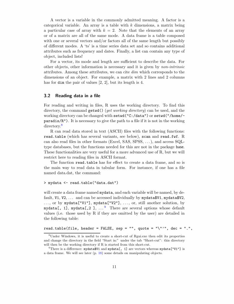
For a vector, its mode and length are sufficient to describe the data. Forother objects, other information is necessary and it is given by non-intrinsicattributes. Among these attributes, we can cite dim which corresponds to thedimensions of an object. For example, a matrix with 2 lines and 2 columnshas for dim the pair of values [2, 2], but its length is 4.
3.2 Reading data in a file
For reading and writing in files, R uses the working directory. To find thisdirectory, the command getwd() (get working directory) can be used, and theworking directory can be changed with setwd("C:/data") or setwd("/home/-paradis/R"). It is necessary to give the path to a file if it is not in the workingdirectory.8
R can read data stored in text (ASCII) files with the following functions:read.table (which has several variants, see below), scan and read.fwf. Rcan also read files in other formats (Excel, SAS, SPSS, . . . ), and access SQL-type databases, but the functions needed for this are not in the package base.These functionalities are very useful for a more advanced use of R, but we willrestrict here to reading files in ASCII format.
The function read.table has for effect to create a data frame, and so isthe main way to read data in tabular form. For instance, if one has a filenamed data.dat, the command:
> mydata <- read.table("data.dat")
will create a data frame named mydata, and each variable will be named, by de-fault, V1, V2, . . . and can be accessed individually by mydata$V1, mydata$V2,. . . , or by mydata["V1"], mydata["V2"], . . . , or, still another solution, bymydata[, 1], mydata[,2 ], . . . 9 There are several options whose defaultvalues (i.e. those used by R if they are omitted by the user) are detailed inthe following table:
read.table(file, header = FALSE, sep = "", quote = "\"’", dec = ".",
8Under Windows, it is useful to create a short-cut of Rgui.exe then edit its propertiesand change the directory in the field “Start in:” under the tab “Short-cut”: this directorywill then be the working directory if R is started from this short-cut.
9There is a difference: mydata$V1 and mydata[, 1] are vectors whereas mydata["V1"] isa data frame. We will see later (p. 18) some details on manipulating objects.
11
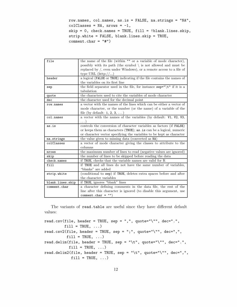
row.names, col.names, as.is = FALSE, na.strings = "NA",
colClasses = NA, nrows = -1,
skip = 0, check.names = TRUE, fill = !blank.lines.skip,
strip.white = FALSE, blank.lines.skip = TRUE,
comment.char = "#")
file the name of the file (within "" or a variable of mode character),possibly with its path (the symbol \ is not allowed and must bereplaced by /, even under Windows), or a remote access to a file oftype URL (http://...)
header a logical (FALSE or TRUE) indicating if the file contains the names ofthe variables on its first line
sep the field separator used in the file, for instance sep="\t" if it is atabulation
quote the characters used to cite the variables of mode character
dec the character used for the decimal point
row.names a vector with the names of the lines which can be either a vector ofmode character, or the number (or the name) of a variable of thefile (by default: 1, 2, 3, . . . )
col.names a vector with the names of the variables (by default: V1, V2, V3,. . . )
as.is controls the conversion of character variables as factors (if FALSE)or keeps them as characters (TRUE); as.is can be a logical, numericor character vector specifying the variables to be kept as character
na.strings the value given to missing data (converted as NA)
colClasses a vector of mode character giving the classes to attribute to thecolumns
nrows the maximum number of lines to read (negative values are ignored)
skip the number of lines to be skipped before reading the data
check.names if TRUE, checks that the variable names are valid for R
fill if TRUE and all lines do not have the same number of variables,“blanks” are added
strip.white (conditional to sep) if TRUE, deletes extra spaces before and afterthe character variables
blank.lines.skip if TRUE, ignores “blank” lines
comment.char a character defining comments in the data file, the rest of theline after this character is ignored (to disable this argument, usecomment.char = "")
The variants of read.table are useful since they have different defaultvalues:
read.csv(file, header = TRUE, sep = ",", quote="\"", dec=".",
fill = TRUE, ...)
read.csv2(file, header = TRUE, sep = ";", quote="\"", dec=",",
fill = TRUE, ...)
read.delim(file, header = TRUE, sep = "\t", quote="\"", dec=".",
fill = TRUE, ...)
read.delim2(file, header = TRUE, sep = "\t", quote="\"", dec=",",
fill = TRUE, ...)
12

The function scan is more flexible than read.table. A difference is thatit is possible to specify the mode of the variables, for example:
> mydata <- scan("data.dat", what = list("", 0, 0))
reads in the file data.dat three variables, the first is of mode character and thenext two are of mode numeric. Another important distinction is that scan()can be used to create different objects, vectors, matrices, data frames, lists,. . . In the above example, mydata is a list of three vectors. By default, that isif what is omitted, scan() creates a numeric vector. If the data read do notcorrespond to the mode(s) expected (either by default, or specified by what),an error message is returned. The options are the followings.
scan(file = "", what = double(0), nmax = -1, n = -1, sep = "",
quote = if (sep=="\n") "" else "’\"", dec = ".",
skip = 0, nlines = 0, na.strings = "NA",
flush = FALSE, fill = FALSE, strip.white = FALSE, quiet = FALSE,
blank.lines.skip = TRUE, multi.line = TRUE, comment.char = "",
allowEscapes = TRUE)
file the name of the file (within ""), possibly with its path (the symbol\ is not allowed and must be replaced by /, even under Windows),or a remote access to a file of type URL (http://...); if file="", thedata are entered with the keyboard (the entree is terminated by ablank line)
what specifies the mode(s) of the data (numeric by default)
nmax the number of data to read, or, if what is a list, the number of linesto read (by default, scan reads the data up to the end of file)
n the number of data to read (by default, no limit)
sep the field separator used in the file
quote the characters used to cite the variables of mode character
dec the character used for the decimal point
skip the number of lines to be skipped before reading the data
nlines the number of lines to read
na.string the value given to missing data (converted as NA)
flush a logical, if TRUE, scan goes to the next line once the number ofcolumns has been reached (allows the user to add comments in thedata file)
fill if TRUE and all lines do not have the same number of variables,“blanks” are added
strip.white (conditional to sep) if TRUE, deletes extra spaces before and afterthe character variables
quiet a logical, if FALSE, scan displays a line showing which fields havebeen read
blank.lines.skip if TRUE, ignores blank lines
multi.line if what is a list, specifies if the variables of the same individual areon a single line in the file (FALSE)
comment.char a character defining comments in the data file, the rest of the lineafter this character is ignored (the default is to have this disabled)
allowEscapes specifies whether C-style escapes (e.g., ‘\t’) be processed (the de-fault) or read as verbatim
13

The function read.fwf can be used to read in a file some data in fixedwidth format :
read.fwf(file, widths, header = FALSE, sep = "\t",
as.is = FALSE, skip = 0, row.names, col.names,
n = -1, buffersize = 2000, ...)
The options are the same than for read.table() ex-cept widths which specifies the width of the fields(buffersize is the maximum number of lines read si-multaneously). For example, if a file named data.txt hasthe data indicated on the right, one can read the datawith the following command:
A1.501.2
A1.551.3
B1.601.4
B1.651.5
C1.701.6
C1.751.7
> mydata <- read.fwf("data.txt", widths=c(1, 4, 3))
> mydata
V1 V2 V3
1 A 1.50 1.2
2 A 1.55 1.3
3 B 1.60 1.4
4 B 1.65 1.5
5 C 1.70 1.6
6 C 1.75 1.7
3.3 Saving data
The function write.tablewrites in a file an object, typically a data frame butthis could well be another kind of object (vector, matrix, . . . ). The argumentsand options are:
write.table(x, file = "", append = FALSE, quote = TRUE, sep = " ",
eol = "\n", na = "NA", dec = ".", row.names = TRUE,
col.names = TRUE, qmethod = c("escape", "double"))
x the name of the object to be written
file the name of the file (by default the object is displayed on the screen)
append if TRUE adds the data without erasing those possibly existing in the file
quote a logical or a numeric vector: if TRUE the variables of mode character andthe factors are written within "", otherwise the numeric vector indicatesthe numbers of the variables to write within "" (in both cases the namesof the variables are written within "" but not if quote = FALSE)
sep the field separator used in the file
eol the character to be used at the end of each line ("\n" is a carriage-return)
na the character to be used for missing data
dec the character used for the decimal point
row.names a logical indicating whether the names of the lines are written in the file
col.names id. for the names of the columns
qmethod specifies, if quote=TRUE, how double quotes " included in variables of modecharacter are treated: if "escape" (or "e", the default) each " is replacedby \", if "d" each " is replaced by ""
14

To write in a simpler way an object in a file, the command write(x,
file="data.txt") can be used, where x is the name of the object (whichcan be a vector, a matrix, or an array). There are two options: nc (or ncol)which defines the number of columns in the file (by default nc=1 if x is of modecharacter, nc=5 for the other modes), and append (a logical) to add the datawithout deleting those possibly already in the file (TRUE) or deleting them ifthe file already exists (FALSE, the default).
To record a group of objects of any type, we can use the command save(x,
y, z, file= "xyz.RData"). To ease the transfert of data between differ-ent machines, the option ascii = TRUE can be used. The data (which arenow called a workspace in R’s jargon) can be loaded later in memory withload("xyz.RData"). The function save.image() is a short-cut for save(list=ls(all=TRUE), file=".RData").
3.4 Generating data
3.4.1 Regular sequences
A regular sequence of integers, for example from 1 to 30, can be generatedwith:
> x <- 1:30
The resulting vector x has 30 elements. The operator ‘:’ has priority on thearithmetic operators within an expression:
> 1:10-1
[1] 0 1 2 3 4 5 6 7 8 9
> 1:(10-1)
[1] 1 2 3 4 5 6 7 8 9
The function seq can generate sequences of real numbers as follows:
> seq(1, 5, 0.5)
[1] 1.0 1.5 2.0 2.5 3.0 3.5 4.0 4.5 5.0
where the first number indicates the beginning of the sequence, the second onethe end, and the third one the increment to be used to generate the sequence.One can use also:
> seq(length=9, from=1, to=5)
[1] 1.0 1.5 2.0 2.5 3.0 3.5 4.0 4.5 5.0
One can also type directly the values using the function c:
> c(1, 1.5, 2, 2.5, 3, 3.5, 4, 4.5, 5)
[1] 1.0 1.5 2.0 2.5 3.0 3.5 4.0 4.5 5.0
15

It is also possible, if one wants to enter some data on the keyboard, to usethe function scan with simply the default options:
> z <- scan()
1: 1.0 1.5 2.0 2.5 3.0 3.5 4.0 4.5 5.0
10:
Read 9 items
> z
[1] 1.0 1.5 2.0 2.5 3.0 3.5 4.0 4.5 5.0
The function rep creates a vector with all its elements identical:
> rep(1, 30)
[1] 1 1 1 1 1 1 1 1 1 1 1 1 1 1 1 1 1 1 1 1 1 1 1 1 1 1 1 1 1 1
The function sequence creates a series of sequences of integers each endingby the numbers given as arguments:
> sequence(4:5)
[1] 1 2 3 4 1 2 3 4 5
> sequence(c(10,5))
[1] 1 2 3 4 5 6 7 8 9 10 1 2 3 4 5
The function gl (generate levels) is very useful because it generates regularseries of factors. The usage of this fonction is gl(k, n) where k is the numberof levels (or classes), and n is the number of replications in each level. Twooptions may be used: length to specify the number of data produced, andlabels to specify the names of the levels of the factor. Examples:
> gl(3, 5)
[1] 1 1 1 1 1 2 2 2 2 2 3 3 3 3 3
Levels: 1 2 3
> gl(3, 5, length=30)
[1] 1 1 1 1 1 2 2 2 2 2 3 3 3 3 3 1 1 1 1 1 2 2 2 2 2 3 3 3 3 3
Levels: 1 2 3
> gl(2, 6, label=c("Male", "Female"))
[1] Male Male Male Male Male Male
[7] Female Female Female Female Female Female
Levels: Male Female
> gl(2, 10)
[1] 1 1 1 1 1 1 1 1 1 1 2 2 2 2 2 2 2 2 2 2
Levels: 1 2
> gl(2, 1, length=20)
[1] 1 2 1 2 1 2 1 2 1 2 1 2 1 2 1 2 1 2 1 2
Levels: 1 2
> gl(2, 2, length=20)
[1] 1 1 2 2 1 1 2 2 1 1 2 2 1 1 2 2 1 1 2 2
Levels: 1 2
16

Finally, expand.grid() creates a data frame with all combinations of vec-tors or factors given as arguments:
> expand.grid(h=c(60,80), w=c(100, 300), sex=c("Male", "Female"))
h w sex
1 60 100 Male
2 80 100 Male
3 60 300 Male
4 80 300 Male
5 60 100 Female
6 80 100 Female
7 60 300 Female
8 80 300 Female
3.4.2 Random sequences
law function
Gaussian (normal) rnorm(n, mean=0, sd=1)
exponential rexp(n, rate=1)
gamma rgamma(n, shape, scale=1)
Poisson rpois(n, lambda)
Weibull rweibull(n, shape, scale=1)
Cauchy rcauchy(n, location=0, scale=1)
beta rbeta(n, shape1, shape2)
‘Student’ (t) rt(n, df)
Fisher–Snedecor (F ) rf(n, df1, df2)
Pearson (χ2) rchisq(n, df)
binomial rbinom(n, size, prob)
multinomial rmultinom(n, size, prob)
geometric rgeom(n, prob)
hypergeometric rhyper(nn, m, n, k)
logistic rlogis(n, location=0, scale=1)
lognormal rlnorm(n, meanlog=0, sdlog=1)
negative binomial rnbinom(n, size, prob)
uniform runif(n, min=0, max=1)
Wilcoxon’s statistics rwilcox(nn, m, n), rsignrank(nn, n)
It is useful in statistics to be able to generate random data, and R cando it for a large number of probability density functions. These functions areof the form rfunc(n, p1, p2, ...), where func indicates the probabilitydistribution, n the number of data generated, and p1, p2, . . . are the values ofthe parameters of the distribution. The above table gives the details for eachdistribution, and the possible default values (if none default value is indicated,this means that the parameter must be specified by the user).
Most of these functions have counterparts obtained by replacing the letterr with d, p or q to get, respectively, the probability density (dfunc(x, ...)),
17

the cumulative probability density (pfunc(x, ...)), and the value of quantile(qfunc(p, ...), with 0 < p < 1). The last two series of functions can beused to find critical values or P -values of statistical tests. For instance, thecritical values for a two-tailed test following a normal distribution at the 5%threshold are:
> qnorm(0.025)
[1] -1.959964
> qnorm(0.975)
[1] 1.959964
For the one-tailed version of the same test, either qnorm(0.05) or 1 -
qnorm(0.95) will be used depending on the form of the alternative hypothesis.The P -value of a test, say χ2 = 3.84 with df = 1, is:
> 1 - pchisq(3.84, 1)
[1] 0.05004352
3.5 Manipulating objects
3.5.1 Creating objects
We have seen previously different ways to create objects using the assign op-erator; the mode and the type of objects so created are generally determinedimplicitly. It is possible to create an object and specifying its mode, length,type, etc. This approach is interesting in the perspective of manipulating ob-jects. One can, for instance, create an ‘empty’ object and then modify itselements successively which is more efficient than putting all its elements to-gether with c(). The indexing system could be used here, as we will see later(p. 26).
It can also be very convenient to create objects from others. For example,if one wants to fit a series of models, it is simple to put the formulae in a list,and then to extract the elements successively to insert them in the functionlm.
At this stage of our learning of R, the interest in learning the followingfunctionalities is not only practical but also didactic. The explicit constructionof objects gives a better understanding of their structure, and allows us to gofurther in some notions previously mentioned.
Vector. The function vector, which has two arguments mode and length,creates a vector which elements have a value depending on the modespecified as argument: 0 if numeric, FALSE if logical, or "" if charac-ter. The following functions have exactly the same effect and have forsingle argument the length of the vector: numeric(), logical(), andcharacter().
18

Factor. A factor includes not only the values of the corresponding categoricalvariable, but also the different possible levels of that variable (even if theyare not present in the data). The function factor creates a factor withthe following options:
factor(x, levels = sort(unique(x), na.last = TRUE),
labels = levels, exclude = NA, ordered = is.ordered(x))
levels specifies the possible levels of the factor (by default the uniquevalues of the vector x), labels defines the names of the levels, excludethe values of x to exclude from the levels, and ordered is a logicalargument specifying whether the levels of the factor are ordered. Recallthat x is of mode numeric or character. Some examples follow.
> factor(1:3)
[1] 1 2 3
Levels: 1 2 3
> factor(1:3, levels=1:5)
[1] 1 2 3
Levels: 1 2 3 4 5
> factor(1:3, labels=c("A", "B", "C"))
[1] A B C
Levels: A B C
> factor(1:5, exclude=4)
[1] 1 2 3 NA 5
Levels: 1 2 3 5
The function levels extracts the possible levels of a factor:
> ff <- factor(c(2, 4), levels=2:5)
> ff
[1] 2 4
Levels: 2 3 4 5
> levels(ff)
[1] "2" "3" "4" "5"
Matrix. A matrix is actually a vector with an additional attribute (dim)which is itself a numeric vector with length 2, and defines the numbersof rows and columns of the matrix. A matrix can be created with thefunction matrix:
matrix(data = NA, nrow = 1, ncol = 1, byrow = FALSE,
dimnames = NULL)
19

The option byrow indicates whether the values given by data must fillsuccessively the columns (the default) or the rows (if TRUE). The optiondimnames allows to give names to the rows and columns.
> matrix(data=5, nr=2, nc=2)
[,1] [,2]
[1,] 5 5
[2,] 5 5
> matrix(1:6, 2, 3)
[,1] [,2] [,3]
[1,] 1 3 5
[2,] 2 4 6
> matrix(1:6, 2, 3, byrow=TRUE)
[,1] [,2] [,3]
[1,] 1 2 3
[2,] 4 5 6
Another way to create a matrix is to give the appropriate values to thedim attribute (which is initially NULL):
> x <- 1:15
> x
[1] 1 2 3 4 5 6 7 8 9 10 11 12 13 14 15
> dim(x)
NULL
> dim(x) <- c(5, 3)
> x
[,1] [,2] [,3]
[1,] 1 6 11
[2,] 2 7 12
[3,] 3 8 13
[4,] 4 9 14
[5,] 5 10 15
Data frame. We have seen that a data frame is created implicitly by thefunction read.table; it is also possible to create a data frame with thefunction data.frame. The vectors so included in the data frame mustbe of the same length, or if one of the them is shorter, it is “recycled” awhole number of times:
> x <- 1:4; n <- 10; M <- c(10, 35); y <- 2:4
> data.frame(x, n)
x n
1 1 10
2 2 10
20

3 3 10
4 4 10
> data.frame(x, M)
x M
1 1 10
2 2 35
3 3 10
4 4 35
> data.frame(x, y)
Error in data.frame(x, y) :
arguments imply differing number of rows: 4, 3
If a factor is included in a data frame, it must be of the same length thanthe vector(s). It is possible to change the names of the columns with,for instance, data.frame(A1=x, A2=n). One can also give names to therows with the option row.names which must be, of course, a vector ofmode character and of length equal to the number of lines of the dataframe. Finally, note that data frames have an attribute dim similarly tomatrices.
List. A list is created in a way similar to data frames with the function list.There is no constraint on the objects that can be included. In contrastto data.frame(), the names of the objects are not taken by default;taking the vectors x and y of the previous example:
> L1 <- list(x, y); L2 <- list(A=x, B=y)
> L1
[[1]]
[1] 1 2 3 4
[[2]]
[1] 2 3 4
> L2
$A
[1] 1 2 3 4
$B
[1] 2 3 4
> names(L1)
NULL
> names(L2)
[1] "A" "B"
Time-series. The function ts creates an object of class "ts" from a vector(single time-series) or a matrix (multivariate time-series), and some op-
21

tions which characterize the series. The options, with the default values,are:
ts(data = NA, start = 1, end = numeric(0), frequency = 1,
deltat = 1, ts.eps = getOption("ts.eps"), class, names)
data a vector or a matrixstart the time of the first observation, either a number, or a
vector of two integers (see the examples below)end the time of the last observation specified in the same way
than start
frequency the number of observations per time unitdeltat the fraction of the sampling period between successive
observations (ex. 1/12 for monthly data); only one offrequency or deltat must be given
ts.eps tolerance for the comparison of series. The frequenciesare considered equal if their difference is less than ts.eps
class class to give to the object; the default is "ts" for a singleseries, and c("mts", "ts") for a multivariate series
names a vector of mode character with the names of the individ-ual series in the case of a multivariate series; by defaultthe names of the columns of data, or Series 1, Series2, . . .
A few examples of time-series created with ts:
> ts(1:10, start = 1959)
Time Series:
Start = 1959
End = 1968
Frequency = 1
[1] 1 2 3 4 5 6 7 8 9 10
> ts(1:47, frequency = 12, start = c(1959, 2))
Jan Feb Mar Apr May Jun Jul Aug Sep Oct Nov Dec
1959 1 2 3 4 5 6 7 8 9 10 11
1960 12 13 14 15 16 17 18 19 20 21 22 23
1961 24 25 26 27 28 29 30 31 32 33 34 35
1962 36 37 38 39 40 41 42 43 44 45 46 47
> ts(1:10, frequency = 4, start = c(1959, 2))
Qtr1 Qtr2 Qtr3 Qtr4
1959 1 2 3
1960 4 5 6 7
1961 8 9 10
> ts(matrix(rpois(36, 5), 12, 3), start=c(1961, 1), frequency=12)
Series 1 Series 2 Series 3
22

Jan 1961 8 5 4
Feb 1961 6 6 9
Mar 1961 2 3 3
Apr 1961 8 5 4
May 1961 4 9 3
Jun 1961 4 6 13
Jul 1961 4 2 6
Aug 1961 11 6 4
Sep 1961 6 5 7
Oct 1961 6 5 7
Nov 1961 5 5 7
Dec 1961 8 5 2
Expression. The objects of mode expression have a fundamental role in R.An expression is a series of characters which makes sense for R. All validcommands are expressions. When a command is typed directly on thekeyboard, it is then evaluated by R and executed if it is valid. In manycircumstances, it is useful to construct an expression without evaluatingit: this is what the function expression is made for. It is, of course,possible to evaluate the expression subsequently with eval().
> x <- 3; y <- 2.5; z <- 1
> exp1 <- expression(x / (y + exp(z)))
> exp1
expression(x/(y + exp(z)))
> eval(exp1)
[1] 0.5749019
Expressions can be used, among other things, to include equations ingraphs (p. 42). An expression can be created from a variable of modecharacter. Some functions take expressions as arguments, for example D
which returns partial derivatives:
> D(exp1, "x")
1/(y + exp(z))
> D(exp1, "y")
-x/(y + exp(z))^2
> D(exp1, "z")
-x * exp(z)/(y + exp(z))^2
3.5.2 Converting objects
The reader has surely realized that the differences between some types ofobjects are small; it is thus logical that it is possible to convert an object froma type to another by changing some of its attributes. Such a conversion will bedone with a function of the type as.something . R (version 2.1.0) has, in the
23

packages base and utils, 98 of such functions, so we will not go in the deepestdetails here.
The result of a conversion depends obviously of the attributes of the con-verted object. Genrally, conversion follows intuitive rules. For the conversionof modes, the following table summarizes the situation.
Conversion to Function Rules
numeric as.numeric FALSE → 0TRUE → 1
"1", "2", . . . → 1, 2, . . ."A", . . . → NA
logical as.logical 0 → FALSE
other numbers → TRUE
"FALSE", "F" → FALSE
"TRUE", "T" → TRUE
other characters → NA
character as.character 1, 2, . . . → "1", "2", . . .FALSE → "FALSE"
TRUE → "TRUE"
There are functions to convert the types of objects (as.matrix, as.ts,as.data.frame, as.expression, . . . ). These functions will affect attributesother than the modes during the conversion. The results are, again, generallyintuitive. A situation frequently encountered is the conversion of factors intonumeric values. In this case, R does the conversion with the numeric codingof the levels of the factor:
> fac <- factor(c(1, 10))
> fac
[1] 1 10
Levels: 1 10
> as.numeric(fac)
[1] 1 2
This makes sense when considering a factor of mode character:
> fac2 <- factor(c("Male", "Female"))
> fac2
[1] Male Female
Levels: Female Male
> as.numeric(fac2)
[1] 2 1
Note that the result is not NA as may have been expected from the tableabove.
24

To convert a factor of mode numeric into a numeric vector but keeping thelevels as they are originally specified, one must first convert into character,then into numeric.
> as.numeric(as.character(fac))
[1] 1 10
This procedure is very useful if in a file a numeric variable has also non-numeric values. We have seen that read.table() in such a situation will, bydefault, read this column as a factor.
3.5.3 Operators
We have seen previously that there are three main types of operators in R10.Here is the list.
Operators
Arithmetic Comparison Logical
+ addition < lesser than ! x logical NOT- subtraction > greater than x & y logical AND* multiplication <= lesser than or equal to x && y id./ division >= greater than or equal to x | y logical OR^ power == equal x || y id.%% modulo != different xor(x, y) exclusive OR%/% integer division
The arithmetic and comparison operators act on two elements (x + y, a< b). The arithmetic operators act not only on variables of mode numeric orcomplex, but also on logical variables; in this latter case, the logical valuesare coerced into numeric. The comparison operators may be applied to anymode: they return one or several logical values.
The logical operators are applied to one (!) or two objects of mode logical,and return one (or several) logical values. The operators “AND” and “OR”exist in two forms: the single one operates on each elements of the objects andreturns as many logical values as comparisons done; the double one operateson the first element of the objects.
It is necessary to use the operator “AND” to specify an inequality of thetype 0 < x < 1 which will be coded with: 0 < x & x < 1. The expression 0
< x < 1 is valid, but will not return the expected result: since both operatorsare the same, they are executed successively from left to right. The comparison0 < x is first done and returns a logical value which is then compared to 1(TRUE or FALSE < 1): in this situation, the logical value is implicitly coercedinto numeric (1 or 0 < 1).
10The following characters are also operators for R: $, @, [, [[, :, ?, <-, <<-, =, ::. Atable of operators describing precedence rules can be found with ?Syntax.
25

> x <- 0.5
> 0 < x < 1
[1] FALSE
The comparison operators operate on each element of the two objectsbeing compared (recycling the values of the shortest one if necessary), andthus returns an object of the same size. To compare ‘wholly’ two objects, twofunctions are available: identical and all.equal.
> x <- 1:3; y <- 1:3
> x == y
[1] TRUE TRUE TRUE
> identical(x, y)
[1] TRUE
> all.equal(x, y)
[1] TRUE
identical compares the internal representation of the data and returnsTRUE if the objects are strictly identical, and FALSE otherwise. all.equal
compares the “near equality” of two objects, and returns TRUE or display asummary of the differences. The latter function takes the approximation ofthe computing process into account when comparing numeric values. Thecomparison of numeric values on a computer is sometimes surprising!
> 0.9 == (1 - 0.1)
[1] TRUE
> identical(0.9, 1 - 0.1)
[1] TRUE
> all.equal(0.9, 1 - 0.1)
[1] TRUE
> 0.9 == (1.1 - 0.2)
[1] FALSE
> identical(0.9, 1.1 - 0.2)
[1] FALSE
> all.equal(0.9, 1.1 - 0.2)
[1] TRUE
> all.equal(0.9, 1.1 - 0.2, tolerance = 1e-16)
[1] "Mean relative difference: 1.233581e-16"
3.5.4 Accessing the values of an object: the indexing system
The indexing system is an efficient and flexible way to access selectively theelements of an object; it can be either numeric or logical. To access, forexample, the third value of a vector x, we just type x[3] which can be usedeither to extract or to change this value:
> x <- 1:5
26

> x[3]
[1] 3
> x[3] <- 20
> x
[1] 1 2 20 4 5
The index itself can be a vector of mode numeric:
> i <- c(1, 3)
> x[i]
[1] 1 20
If x is a matrix or a data frame, the value of the ith line and j th columnis accessed with x[i, j]. To access all values of a given row or column, onehas simply to omit the appropriate index (without forgetting the comma!):
> x <- matrix(1:6, 2, 3)
> x
[,1] [,2] [,3]
[1,] 1 3 5
[2,] 2 4 6
> x[, 3] <- 21:22
> x
[,1] [,2] [,3]
[1,] 1 3 21
[2,] 2 4 22
> x[, 3]
[1] 21 22
You have certainly noticed that the last result is a vector and not a matrix.The default behaviour of R is to return an object of the lowest dimensionpossible. This can be altered with the option drop which default is TRUE:
> x[, 3, drop = FALSE]
[,1]
[1,] 21
[2,] 22
This indexing system is easily generalized to arrays, with as many indicesas the number of dimensions of the array (for example, a three dimensionalarray: x[i, j, k], x[, , 3], x[, , 3, drop = FALSE], and so on). It maybe useful to keep in mind that indexing is made with square brackets, whileparentheses are used for the arguments of a function:
> x(1)
Error: couldn’t find function "x"
27

Indexing can also be used to suppress one or several rows or columnsusing negative values. For example, x[-1, ] will suppress the first row, whilex[-c(1, 15), ] will do the same for the 1st and 15th rows. Using the matrixdefined above:
> x[, -1]
[,1] [,2]
[1,] 3 21
[2,] 4 22
> x[, -(1:2)]
[1] 21 22
> x[, -(1:2), drop = FALSE]
[,1]
[1,] 21
[2,] 22
For vectors, matrices and arrays, it is possible to access the values of anelement with a comparison expression as the index:
> x <- 1:10
> x[x >= 5] <- 20
> x
[1] 1 2 3 4 20 20 20 20 20 20
> x[x == 1] <- 25
> x
[1] 25 2 3 4 20 20 20 20 20 20
A practical use of the logical indexing is, for instance, the possibility toselect the even elements of an integer variable:
> x <- rpois(40, lambda=5)
> x
[1] 5 9 4 7 7 6 4 5 11 3 5 7 1 5 3 9 2 2 5 2
[21] 4 6 6 5 4 5 3 4 3 3 3 7 7 3 8 1 4 2 1 4
> x[x %% 2 == 0]
[1] 4 6 4 2 2 2 4 6 6 4 4 8 4 2 4
Thus, this indexing system uses the logical values returned, in the aboveexamples, by comparison operators. These logical values can be computedbeforehand, they then will be recycled if necessary:
> x <- 1:40
> s <- c(FALSE, TRUE)
> x[s]
[1] 2 4 6 8 10 12 14 16 18 20 22 24 26 28 30 32 34 36 38 40
28

Logical indexing can also be used with data frames, but with caution sincedifferent columns of the data drame may be of different modes.
For lists, accessing the different elements (which can be any kind of object)is done either with single or with double square brackets: the difference isthat with single brackets a list is returned, whereas double brackets extract theobject from the list. The result can then be itself indexed as previously seen forvectors, matrices, etc. For instance, if the third object of a list is a vector, itsith value can be accessed using my.list[[3]][i], if it is a three dimensionalarray using my.list[[3]][i, j, k], and so on. Another difference is thatmy.list[1:2] will return a list with the first and second elements of theoriginal list, whereas my.list[[1:2]] will no not give the expected result.
3.5.5 Accessing the values of an object with names
The names are labels of the elements of an object, and thus of mode charac-ter. They are generally optional attributes. There are several kinds of names(names, colnames, rownames, dimnames).
The names of a vector are stored in a vector of the same length of theobject, and can be accessed with the function names.
> x <- 1:3
> names(x)
NULL
> names(x) <- c("a", "b", "c")
> x
a b c
1 2 3
> names(x)
[1] "a" "b" "c"
> names(x) <- NULL
> x
[1] 1 2 3
For matrices and data frames, colnames and rownames are labels of thecolumns and rows, respectively. They can be accessed either with their re-spective functions, or with dimnames which returns a list with both vectors.
> X <- matrix(1:4, 2)
> rownames(X) <- c("a", "b")
> colnames(X) <- c("c", "d")
> X
c d
a 1 3
b 2 4
> dimnames(X)
[[1]]
[1] "a" "b"
29

[[2]]
[1] "c" "d"
For arrays, the names of the dimensions can be accessed with dimnames:
> A <- array(1:8, dim = c(2, 2, 2))
> A
, , 1
[,1] [,2]
[1,] 1 3
[2,] 2 4
, , 2
[,1] [,2]
[1,] 5 7
[2,] 6 8
> dimnames(A) <- list(c("a", "b"), c("c", "d"), c("e", "f"))
> A
, , e
c d
a 1 3
b 2 4
, , f
c d
a 5 7
b 6 8
If the elements of an object have names, they can be extracted by usingthem as indices. Actually, this should be termed ‘subsetting’ rather than‘extraction’ since the attributes of the original object are kept. For instance,if a data frame DF contains the variables x, y, and z, the command DF["x"]
will return a data frame with just x; DF[c("x", "y")] will return a dataframe with both variables. This works with lists as well if the elements in thelist have names.
As the reader surely realizes, the index used here is a vector of modecharacter. Like the numeric or logical vectors seen above, this vector can bedefined beforehand and then used for the extraction.
To extract a vector or a factor from a data frame, on can use the operator$ (e.g., DF$x). This also works with lists.
30

3.5.6 The data editor
It is possible to use a graphical spreadsheet-like editor to edit a “data” object.For example, if X is a matrix, the command data.entry(X)will open a graphiceditor and one will be able to modify some values by clicking on the appropriatecells, or to add new columns or rows.
The function data.entry modifies directly the object given as argumentwithout needing to assign its result. On the other hand, the function de
returns a list with the objects given as arguments and possibly modified. Thisresult is displayed on the screen by default, but, as for most functions, can beassigned to an object.
The details of using the data editor depend on the operating system.
3.5.7 Arithmetics and simple functions
There are numerous functions in R to manipulate data. We have already seenthe simplest one, c which concatenates the objects listed in parentheses. Forexample:
> c(1:5, seq(10, 11, 0.2))
[1] 1.0 2.0 3.0 4.0 5.0 10.0 10.2 10.4 10.6 10.8 11.0
Vectors can be manipulated with classical arithmetic expressions:
> x <- 1:4
> y <- rep(1, 4)
> z <- x + y
> z
[1] 2 3 4 5
Vectors of different lengths can be added; in this case, the shortest vectoris recycled. Examples:
> x <- 1:4
> y <- 1:2
> z <- x + y
> z
[1] 2 4 4 6
> x <- 1:3
> y <- 1:2
> z <- x + y
Warning message:
longer object length
is not a multiple of shorter object length in: x + y
> z
[1] 2 4 4
31

Note that R returned a warning message and not an error message, thusthe operation has been performed. If we want to add (or multiply) the samevalue to all the elements of a vector:
> x <- 1:4
> a <- 10
> z <- a * x
> z
[1] 10 20 30 40
The functions available in R for manipulating data are too many to belisted here. One can find all the basic mathematical functions (log, exp,log10, log2, sin, cos, tan, asin, acos, atan, abs, sqrt, . . . ), special func-tions (gamma, digamma, beta, besselI, . . . ), as well as diverse functions usefulin statistics. Some of these functions are listed in the following table.
sum(x) sum of the elements of x
prod(x) product of the elements of x
max(x) maximum of the elements of x
min(x) minimum of the elements of x
which.max(x) returns the index of the greatest element of x
which.min(x) returns the index of the smallest element of x
range(x) id. than c(min(x), max(x))
length(x) number of elements in x
mean(x) mean of the elements of x
median(x) median of the elements of x
var(x) or cov(x) variance of the elements of x (calculated on n − 1); if x isa matrix or a data frame, the variance-covariance matrix iscalculated
cor(x) correlation matrix of x if it is a matrix or a data frame (1 if xis a vector)
var(x, y) or cov(x, y) covariance between x and y, or between the columns of x andthose of y if they are matrices or data frames
cor(x, y) linear correlation between x and y, or correlation matrix if theyare matrices or data frames
These functions return a single value (thus a vector of length one), exceptrange which returns a vector of length two, and var, cov, and cor which mayreturn a matrix. The following functions return more complex results.
round(x, n) rounds the elements of x to n decimals
rev(x) reverses the elements of x
sort(x) sorts the elements of x in increasing order; to sort in decreasing order:rev(sort(x))
rank(x) ranks of the elements of x
32

log(x, base) computes the logarithm of x with base base
scale(x) if x is a matrix, centers and reduces the data; to center only usethe option center=FALSE, to reduce only scale=FALSE (by defaultcenter=TRUE, scale=TRUE)
pmin(x,y,...) a vector which ith element is the minimum of x[i], y[i], . . .
pmax(x,y,...) id. for the maximum
cumsum(x) a vector which ith element is the sum from x[1] to x[i]
cumprod(x) id. for the product
cummin(x) id. for the minimum
cummax(x) id. for the maximum
match(x, y) returns a vector of the same length than x with the elements of x
which are in y (NA otherwise)
which(x == a) returns a vector of the indices of x if the comparison operation istrue (TRUE), in this example the values of i for which x[i] == a (theargument of this function must be a variable of mode logical)
choose(n, k) computes the combinations of k events among n repetitions = n!/[(n−k)!k!]
na.omit(x) suppresses the observations with missing data (NA) (suppresses thecorresponding line if x is a matrix or a data frame)
na.fail(x) returns an error message if x contains at least one NA
unique(x) if x is a vector or a data frame, returns a similar object but with theduplicate elements suppressed
table(x) returns a table with the numbers of the differents values of x (typicallyfor integers or factors)
table(x, y) contingency table of x and y
subset(x, ...) returns a selection of x with respect to criteria (..., typically com-parisons: x$V1 < 10); if x is a data frame, the option select givesthe variables to be kept (or dropped using a minus sign)
sample(x, size) resample randomly and without replacement size elements in thevector x, the option replace = TRUE allows to resample with replace-ment
3.5.8 Matrix computation
R has facilities for matrix computation and manipulation. The functionsrbind and cbind bind matrices with respect to the lines or the columns,respectively:
> m1 <- matrix(1, nr = 2, nc = 2)
> m2 <- matrix(2, nr = 2, nc = 2)
> rbind(m1, m2)
[,1] [,2]
[1,] 1 1
[2,] 1 1
[3,] 2 2
[4,] 2 2
> cbind(m1, m2)
[,1] [,2] [,3] [,4]
33

[1,] 1 1 2 2
[2,] 1 1 2 2
The operator for the product of two matrices is ‘%*%’. For example, con-sidering the two matrices m1 and m2 above:
> rbind(m1, m2) %*% cbind(m1, m2)
[,1] [,2] [,3] [,4]
[1,] 2 2 4 4
[2,] 2 2 4 4
[3,] 4 4 8 8
[4,] 4 4 8 8
> cbind(m1, m2) %*% rbind(m1, m2)
[,1] [,2]
[1,] 10 10
[2,] 10 10
The transposition of a matrix is done with the function t; this functionworks also with a data frame.
The function diag can be used to extract or modify the diagonal of amatrix, or to build a diagonal matrix.
> diag(m1)
[1] 1 1
> diag(rbind(m1, m2) %*% cbind(m1, m2))
[1] 2 2 8 8
> diag(m1) <- 10
> m1
[,1] [,2]
[1,] 10 1
[2,] 1 10
> diag(3)
[,1] [,2] [,3]
[1,] 1 0 0
[2,] 0 1 0
[3,] 0 0 1
> v <- c(10, 20, 30)
> diag(v)
[,1] [,2] [,3]
[1,] 10 0 0
[2,] 0 20 0
[3,] 0 0 30
> diag(2.1, nr = 3, nc = 5)
[,1] [,2] [,3] [,4] [,5]
[1,] 2.1 0.0 0.0 0 0
[2,] 0.0 2.1 0.0 0 0
[3,] 0.0 0.0 2.1 0 0
34

R has also some special functions for matrix computation. We can citehere solve for inverting a matrix, qr for decomposition, eigen for computingeigenvalues and eigenvectors, and svd for singular value decomposition.
35

4 Graphics with R
R offers a remarkable variety of graphics. To get an idea, one can typedemo(graphics) or demo(persp). It is not possible to detail here the pos-sibilities of R in terms of graphics, particularly since each graphical functionhas a large number of options making the production of graphics very flexible.
The way graphical functions work deviates substantially from the schemesketched at the beginning of this document. Particularly, the result of a graph-ical function cannot be assigned to an object11 but is sent to a graphical device.A graphical device is a graphical window or a file.
There are two kinds of graphical functions: the high-level plotting func-tions which create a new graph, and the low-level plotting functions whichadd elements to an existing graph. The graphs are produced with respect tographical parameters which are defined by default and can be modified withthe function par.
We will see in a first time how to manage graphics and graphical devices;we will then somehow detail the graphical functions and parameters. We willsee a practical example of the use of these functionalities in producing graphs.Finally, we will see the packages grid and lattice whose functioning is differentfrom the one summarized above.
4.1 Managing graphics
4.1.1 Opening several graphical devices
When a graphical function is executed, if no graphical device is open, R opens agraphical window and displays the graph. A graphical device may be open withan appropriate function. The list of available graphical devices depends on theoperating system. The graphical windows are called X11 under Unix/Linuxand windows under Windows. In all cases, one can open a graphical windowwith the command x11() which also works under Windows because of an aliastowards the command windows(). A graphical device which is a file will beopen with a function depending on the format: postscript(), pdf(), png(),. . . The list of available graphical devices can be found with ?device.
The last open device becomes the active graphical device on which allsubsequent graphs are displayed. The function dev.list() displays the listof open devices:
> x11(); x11(); pdf()
> dev.list()
11There are a few remarkable exceptions: hist() and barplot() produce also numericresults as lists or matrices.
36

X11 X11 pdf
2 3 4
The figures displayed are the device numbers which must be used to changethe active device. To know what is the active device:
> dev.cur()
4
and to change the active device:
> dev.set(3)
X11
3
The function dev.off() closes a device: by default the active device isclosed, otherwise this is the one which number is given as argument to thefunction. R then displays the number of the new active device:
> dev.off(2)
X11
3
> dev.off()
4
Two specific features of the Windows version of R are worth mentioning:a Windows Metafile device can be open with the function win.metafile, anda menu “History” displayed when the graphical window is selected allowingrecording of all graphs drawn during a session (by default, the recording systemis off, the user switches it on by clicking on “Recording” in this menu).
4.1.2 Partitioning a graphic
The function split.screen partitions the active graphical device. For exam-ple:
> split.screen(c(1, 2))
divides the device into two parts which can be selected with screen(1) orscreen(2); erase.screen() deletes the last drawn graph. A part of thedevice can itself be divided with split.screen() leading to the possibility tomake complex arrangements.
These functions are incompatible with others (such as layout or coplot)and must not be used with multiple graphical devices. Their use should belimited, for instance, to graphical exploration of data.
The function layout partitions the active graphic window in several partswhere the graphs will be displayed successively. Its main argument is a ma-trix with integer numbers indicating the numbers of the “sub-windows”. Forexample, to divide the device into four equal parts:
37

> layout(matrix(1:4, 2, 2))
It is of course possible to create this matrix previously allowing to bettervisualize how the device is divided:
> mat <- matrix(1:4, 2, 2)
> mat
[,1] [,2]
[1,] 1 3
[2,] 2 4
> layout(mat)
To actually visualize the partition created, one can use the function layout.show
with the number of sub-windows as argument (here 4). In this example, wewill have:
> layout.show(4)
1
2
3
4
The following examples show some of the possibilities offered by layout().
> layout(matrix(1:6, 3, 2))
> layout.show(6)
1
2
3
4
5
6
> layout(matrix(1:6, 2, 3))
> layout.show(6)
1
2
3
4
5
6
> m <- matrix(c(1:3, 3), 2, 2)
> layout(m)
> layout.show(3)
1
2
3
In all these examples, we have not used the option byrow of matrix(), thesub-windows are thus numbered column-wise; one can just specify matrix(...,
byrow=TRUE) so that the sub-windows are numbered row-wise. The numbers
38

in the matrix may also be given in any order, for example, matrix(c(2, 1,
4, 3), 2, 2).By default, layout() partitions the device with regular heights and widths:
this can be modified with the options widths and heights. These dimensionsare given relatively12. Examples:
> m <- matrix(1:4, 2, 2)
> layout(m, widths=c(1, 3),
heights=c(3, 1))
> layout.show(4)
1
2
3
4
> m <- matrix(c(1,1,2,1),2,2)
> layout(m, widths=c(2, 1),
heights=c(1, 2))
> layout.show(2)
1
2
Finally, the numbers in the matrix can include zeros giving the possibilityto make complex (or even esoterical) partitions.
> m <- matrix(0:3, 2, 2)
> layout(m, c(1, 3), c(1, 3))
> layout.show(3)1
2
3
> m <- matrix(scan(), 5, 5)
1: 0 0 3 3 3 1 1 3 3 3
11: 0 0 3 3 3 0 2 2 0 5
21: 4 2 2 0 5
26:
Read 25 items
> layout(m)
> layout.show(5)
1
2
3
4
5
12They can be given in centimetres, see ?layout.
39

4.2 Graphical functions
Here is an overview of the high-level graphical functions in R.
plot(x) plot of the values of x (on the y-axis) ordered on the x-axis
plot(x, y) bivariate plot of x (on the x-axis) and y (on the y-axis)
sunflowerplot(x,
y)
id. but the points with similar coordinates are drawn as a flowerwhich petal number represents the number of points
pie(x) circular pie-chart
boxplot(x) “box-and-whiskers” plot
stripchart(x) plot of the values of x on a line (an alternative to boxplot() forsmall sample sizes)
coplot(x~y | z) bivariate plot of x and y for each value (or interval of values) ofz
interaction.plot
(f1, f2, y)
if f1 and f2 are factors, plots the means of y (on the y-axis) withrespect to the values of f1 (on the x-axis) and of f2 (differentcurves); the option fun allows to choose the summary statisticof y (by default fun=mean)
matplot(x,y) bivariate plot of the first column of x vs. the first one of y, thesecond one of x vs. the second one of y, etc.
dotchart(x) if x is a data frame, plots a Cleveland dot plot (stacked plotsline-by-line and column-by-column)
fourfoldplot(x) visualizes, with quarters of circles, the association between twodichotomous variables for different populations (x must be anarray with dim=c(2, 2, k), or a matrix with dim=c(2, 2) ifk = 1)
assocplot(x) Cohen–Friendly graph showing the deviations from indepen-dence of rows and columns in a two dimensional contingencytable
mosaicplot(x) ‘mosaic’ graph of the residuals from a log-linear regression of acontingency table
pairs(x) if x is a matrix or a data frame, draws all possible bivariate plotsbetween the columns of x
plot.ts(x) if x is an object of class "ts", plot of x with respect to time, xmay be multivariate but the series must have the same frequencyand dates
ts.plot(x) id. but if x is multivariate the series may have different datesand must have the same frequency
hist(x) histogram of the frequencies of x
barplot(x) histogram of the values of x
qqnorm(x) quantiles of x with respect to the values expected under a normallaw
qqplot(x, y) quantiles of y with respect to the quantiles of x
contour(x, y, z) contour plot (data are interpolated to draw the curves), x
and y must be vectors and z must be a matrix so thatdim(z)=c(length(x), length(y)) (x and y may be omitted)
filled.contour (x,
y, z)
id. but the areas between the contours are coloured, and a legendof the colours is drawn as well
image(x, y, z) id. but the actual data are represented with colours
persp(x, y, z) id. but in perspective
stars(x) if x is a matrix or a data frame, draws a graph with segmentsor a star where each row of x is represented by a star and thecolumns are the lengths of the segments
40
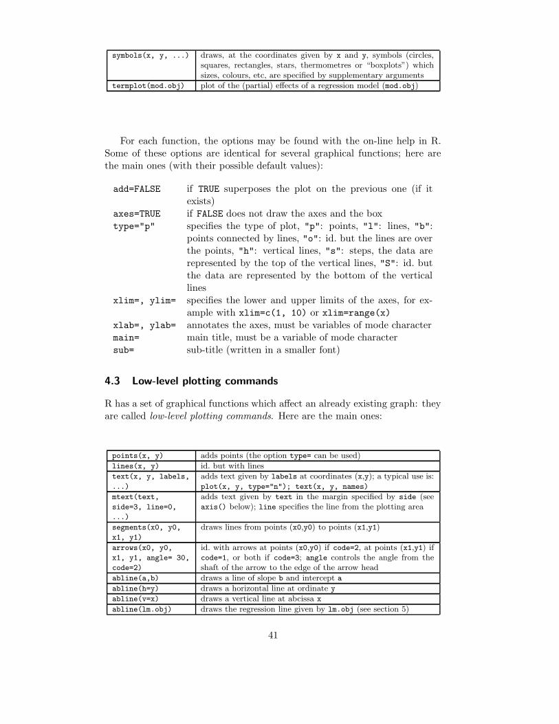
symbols(x, y, ...) draws, at the coordinates given by x and y, symbols (circles,squares, rectangles, stars, thermometres or “boxplots”) whichsizes, colours, etc, are specified by supplementary arguments
termplot(mod.obj) plot of the (partial) effects of a regression model (mod.obj)
For each function, the options may be found with the on-line help in R.Some of these options are identical for several graphical functions; here arethe main ones (with their possible default values):
add=FALSE if TRUE superposes the plot on the previous one (if itexists)
axes=TRUE if FALSE does not draw the axes and the boxtype="p" specifies the type of plot, "p": points, "l": lines, "b":
points connected by lines, "o": id. but the lines are overthe points, "h": vertical lines, "s": steps, the data arerepresented by the top of the vertical lines, "S": id. butthe data are represented by the bottom of the verticallines
xlim=, ylim= specifies the lower and upper limits of the axes, for ex-ample with xlim=c(1, 10) or xlim=range(x)
xlab=, ylab= annotates the axes, must be variables of mode charactermain= main title, must be a variable of mode charactersub= sub-title (written in a smaller font)
4.3 Low-level plotting commands
R has a set of graphical functions which affect an already existing graph: theyare called low-level plotting commands. Here are the main ones:
points(x, y) adds points (the option type= can be used)
lines(x, y) id. but with lines
text(x, y, labels,
...)
adds text given by labels at coordinates (x,y); a typical use is:plot(x, y, type="n"); text(x, y, names)
mtext(text,
side=3, line=0,
...)
adds text given by text in the margin specified by side (seeaxis() below); line specifies the line from the plotting area
segments(x0, y0,
x1, y1)
draws lines from points (x0,y0) to points (x1,y1)
arrows(x0, y0,
x1, y1, angle= 30,
code=2)
id. with arrows at points (x0,y0) if code=2, at points (x1,y1) ifcode=1, or both if code=3; angle controls the angle from theshaft of the arrow to the edge of the arrow head
abline(a,b) draws a line of slope b and intercept a
abline(h=y) draws a horizontal line at ordinate y
abline(v=x) draws a vertical line at abcissa x
abline(lm.obj) draws the regression line given by lm.obj (see section 5)
41

rect(x1, y1, x2,
y2)
draws a rectangle which left, right, bottom, and top limits arex1, x2, y1, and y2, respectively
polygon(x, y) draws a polygon linking the points with coordinates given by x
and y
legend(x, y,
legend)
adds the legend at the point (x,y) with the symbols given bylegend
title() adds a title and optionally a sub-title
axis(side, vect) adds an axis at the bottom (side=1), on the left (2), at the top(3), or on the right (4); vect (optional) gives the abcissa (orordinates) where tick-marks are drawn
box() adds a box around the current plot
rug(x) draws the data x on the x-axis as small vertical lines
locator(n,
type="n", ...)
returns the coordinates (x, y) after the user has clicked n timeson the plot with the mouse; also draws symbols (type="p") orlines (type="l") with respect to optional graphic parameters(...); by default nothing is drawn (type="n")
Note the possibility to add mathematical expressions on a plot with text(x,
y, expression(...)), where the function expression transforms its argu-ment in a mathematical equation. For example,
> text(x, y, expression(p == over(1, 1+e^-(beta*x+alpha))))
will display, on the plot, the following equation at the point of coordinates(x, y):
p =1
1 + e−(βx+α)
To include in an expression a variable we can use the functions substituteand as.expression; for example to include a value of R2 (previously com-puted and stored in an object named Rsquared):
> text(x, y, as.expression(substitute(R^2==r, list(r=Rsquared))))
will display on the plot at the point of coordinates (x, y):
R2 = 0.9856298
To display only three decimals, we can modify the code as follows:
> text(x, y, as.expression(substitute(R^2==r,
+ list(r=round(Rsquared, 3)))))
will display:
R2 = 0.986
Finally, to write the R in italics:
> text(x, y, as.expression(substitute(italic(R)^2==r,
+ list(r=round(Rsquared, 3)))))
R2 = 0.986
42

4.4 Graphical parameters
In addition to low-level plotting commands, the presentation of graphics canbe improved with graphical parameters. They can be used either as optionsof graphic functions (but it does not work for all), or with the function par tochange permanently the graphical parameters, i.e. the subsequent plots willbe drawn with respect to the parameters specified by the user. For instance,the following command:
> par(bg="yellow")
will result in all subsequent plots drawn with a yellow background. Thereare 73 graphical parameters, some of them have very similar functions. Theexhaustive list of these parameters can be read with ?par; I will limit thefollowing table to the most usual ones.
adj controls text justification with respect to the left border of the text so that0 is left-justified, 0.5 is centred, 1 is right-justified, values > 1 move the textfurther to the left, and negative values further to the right; if two values aregiven (e.g., c(0, 0)) the second one controls vertical justification with respectto the text baseline
bg specifies the colour of the background (e.g., bg="red", bg="blue"; the list ofthe 657 available colours is displayed with colors())
bty controls the type of box drawn around the plot, allowed values are: "o","l", "7", "c", "u" ou "]" (the box looks like the corresponding character); ifbty="n" the box is not drawn
cex a value controlling the size of texts and symbols with respect to the default; thefollowing parameters have the same control for numbers on the axes, cex.axis,the axis labels, cex.lab, the title, cex.main, and the sub-title, cex.sub
col controls the colour of symbols; as for cex there are: col.axis, col.lab,col.main, col.sub
font an integer which controls the style of text (1: normal, 2: italics, 3: bold, 4:bold italics); as for cex there are: font.axis, font.lab, font.main, font.sub
las an integer which controls the orientation of the axis labels (0: parallel to theaxes, 1: horizontal, 2: perpendicular to the axes, 3: vertical)
lty controls the type of lines, can be an integer (1: solid, 2: dashed, 3: dotted,4: dotdash, 5: longdash, 6: twodash), or a string of up to eight characters(between "0" and "9") which specifies alternatively the length, in points orpixels, of the drawn elements and the blanks, for example lty="44" will havethe same effet than lty=2
lwd a numeric which controls the width of lines
mar a vector of 4 numeric values which control the space between the axes and theborder of the graph of the form c(bottom, left, top, right), the defaultvalues are c(5.1, 4.1, 4.1, 2.1)
mfcol a vector of the form c(nr,nc) which partitions the graphic window as a ma-trix of nr lines and nc columns, the plots are then drawn in columns (seesection 4.1.2)
mfrow id. but the plots are then drawn in line (see section 4.1.2)
pch controls the type of symbol, either an integer between 1 and 25, or any singlecharacter within "" (Fig. 2)
ps an integer which controls the size in points of texts and symbols
43

* ? X a
1 2 3 4 5 6 7 8 9 10
11 12 13 14 15 16 17 18 19 20
21 22 23 24 25 "*" "?" "." "X" "a"
Figure 2: The plotting symbols in R (pch=1:25). The colours were obtainedwith the options col="blue", bg="yellow", the second option has an effectonly for the symbols 21–25. Any character can be used (pch="*", "?", ".",. . . ).
pty a character which specifies the type of the plotting region, "s": square, "m":maximal
tck a value which specifies the length of tick-marks on the axes as a fraction ofthe smallest of the width or height of the plot; if tck=1 a grid is drawn
tcl id. but as a fraction of the height of a line of text (by default tcl=-0.5)
xaxt if xaxt="n" the x-axis is set but not drawn (useful in conjunction withaxis(side=1, ...))
yaxt if yaxt="n" the y-axis is set but not drawn (useful in conjunction withaxis(side=2, ...))
4.5 A practical example
In order to illustrate R’s graphical functionalities, let us consider a simpleexample of a bivariate graph of 10 pairs of random variates. These valueswere generated with:
> x <- rnorm(10)
> y <- rnorm(10)
The wanted graph will be obtained with plot(); one will type the command:
> plot(x, y)
and the graph will be plotted on the active graphical device. The resultis shown on Fig. 3. By default, R makes graphs in an “intelligent” way:
44

−0.5 0.0 0.5 1.0−
1.0
−0.
50.
00.
5
x
y
Figure 3: The function plot used without options.
the spaces between tick-marks on the axes, the placement of labels, etc, arecalculated so that the resulting graph is as intelligible as possible.
The user may, nevertheless, change the way a graph is presented, for in-stance, to conform to a pre-defined editorial style, or to give it a personaltouch for a talk. The simplest way to change the presentation of a graph is toadd options which will modify the default arguments. In our example, we canmodify significantly the figure in the following way:
plot(x, y, xlab="Ten random values", ylab="Ten other values",
xlim=c(-2, 2), ylim=c(-2, 2), pch=22, col="red",
bg="yellow", bty="l", tcl=0.4,
main="How to customize a plot with R", las=1, cex=1.5)
The result is on Fig. 4. Let us detail each of the used options. First,xlab and ylab change the axis labels which, by default, were the names of thevariables. Then, xlim and ylim allow us to define the limits on both axes13.The graphical parameter pch is used here as an option: pch=22 specifies asquare which contour and background colours may be different and are givenby, respectively, col and bg. The table of graphical parameters gives themeaning of the modifications done by bty, tcl, las and cex. Finally, a titleis added with the option main.
The graphical parameters and the low-level plotting functions allow us togo further in the presentation of a graph. As we have seen previously, somegraphical parameters cannot be passed as arguments to a function like plot.
13By default, R adds 4% on each side of the axis limit. This behaviour may be altered bysetting the graphical parameters xaxs="i" and yaxs="i" (they can be passed as options toplot()).
45

−2 −1 0 1 2
−2
−1
0
1
2
How to customize a plot with R
Ten random values
Ten
oth
er v
alue
s
Figure 4: The function plot used with options.
We will now modify some of these parameters with par(), it is thus necessaryto type several commands. When the graphical parameters are changed, itis useful to save their initial values beforehand to be able to restore themafterwards. Here are the commands used to obtain Fig. 5.
opar <- par()
par(bg="lightyellow", col.axis="blue", mar=c(4, 4, 2.5, 0.25))
plot(x, y, xlab="Ten random values", ylab="Ten other values",
xlim=c(-2, 2), ylim=c(-2, 2), pch=22, col="red", bg="yellow",
bty="l", tcl=-.25, las=1, cex=1.5)
title("How to customize a plot with R (bis)", font.main=3, adj=1)
par(opar)
Let us detail the actions resulting from these commands. First, the defaultgraphical parameters are copied in a list called here opar. Three parameterswill be then modified: bg for the colour of the background, col.axis for thecolour of the numbers on the axes, and mar for the sizes of the margins aroundthe plotting region. The graph is drawn in a nearly similar way to Fig. 4. Themodifications of the margins allowed to use the space around the plotting area.The title here is added with the low-level plotting function title which allowsto give some parameters as arguments without altering the rest of the graph.Finally, the initial graphical parameters are restored with the last command.
Now, total control! On Fig. 5, R still determines a few things such asthe number of tick marks on the axes, or the space between the title and theplotting area. We will see now how to totally control the presentation of thegraph. The approach used here is to plot a “blank” graph with plot(...,
type="n"), then to add points, axes, labels, etc, with low-level plotting func-
46

−2 −1 0 1 2
−2
−1
0
1
2
Ten random values
Ten
oth
er v
alue
s
How to customize a plot with R (bis)
Figure 5: The functions par, plot and title.
tions. We will fancy a few arrangements such as changing the colour of theplotting area. The commands follow, and the resulting graph is on Fig. 6.
opar <- par()
par(bg="lightgray", mar=c(2.5, 1.5, 2.5, 0.25))
plot(x, y, type="n", xlab="", ylab="", xlim=c(-2, 2),
ylim=c(-2, 2), xaxt="n", yaxt="n")
rect(-3, -3, 3, 3, col="cornsilk")
points(x, y, pch=10, col="red", cex=2)
axis(side=1, c(-2, 0, 2), tcl=-0.2, labels=FALSE)
axis(side=2, -1:1, tcl=-0.2, labels=FALSE)
title("How to customize a plot with R (ter)",
font.main=4, adj=1, cex.main=1)
mtext("Ten random values", side=1, line=1, at=1, cex=0.9, font=3)
mtext("Ten other values", line=0.5, at=-1.8, cex=0.9, font=3)
mtext(c(-2, 0, 2), side=1, las=1, at=c(-2, 0, 2), line=0.3,
col="blue", cex=0.9)
mtext(-1:1, side=2, las=1, at=-1:1, line=0.2, col="blue", cex=0.9)
par(opar)
Like before, the default graphical parameters are saved, and the colourof the background and the margins are modified. The graph is then drawnwith type="n" to not plot the points, xlab="", ylab="" to not write theaxis labels, and xaxt="n", yaxt="n" to not draw the axes. This results indrawing only the box around the plotting area, and defining the axes withrespect to xlim et ylim. Note that we could have used the option axes=FALSE
but in this case neither the axes, nor the box would have been drawn.
47

How to customize a plot with R (ter)
Ten random values
Ten other values
−2 0 2
−1
0
1
Figure 6: A “hand-made” graph.
The elements are then added in the plotting region so defined with somelow-level plotting functions. Before adding the points, the colour inside theplotting area is changed with rect(): the size of the rectangle are chosen sothat it is substantially larger than the plotting area.
The points are plotted with points(); a new symbol was used. The axesare added with axis(): the vector given as second argument specifies thecoordinates of the tick-marks. The option labels=FALSE specifies that noannotation must be written with the tick-marks. This option also accepts avector of mode character, for example labels=c("A", "B", "C").
The title is added with title(), but the font is slightly changed. Theannotations on the axes are written with mtext() (marginal text). The firstargument of this function is a vector of mode character giving the text to bewritten. The option line indicates the distance from the plotting area (bydefault line=0), and at the coordinnate. The second call to mtext() usesthe default value of side (3). The two other calls to mtext() pass a numericvector as first argument: this will be converted into character.
4.6 The grid and lattice packages
The packages grid and lattice implement the grid and lattice systems. Grid isa new graphical mode with its own system of graphical parameters which aredistinct from those seen above. The two main distinctions of grid comparedto the base graphics are:
• a more flexible way to split graphical devices using viewports which couldbe overpalling (graphical objects may even be shared among distinctviewports, e.g., arrows);
48

• graphical objects (grob) may be modified or removed from a graph with-out requiring the re-draw all the graph (as must be done with basegraphics).
Grid graphics cannot usually be combined or mixed with base graphics(the gridBase package must be used to do this). However, it is possible to useboth graphical modes in the same session on the same graphical device.
Lattice is essentially the implementation in R of the Trellis graphics ofS-PLUS. Trellis is an approach for visualizing multivariate data which is par-ticularly appropriate for the exploration of relations or interactions amongvariables14. The main idea behind lattice (and Trellis as well) is that of con-ditional multiple graphs: a bivariate graph will be split in several graphs withrespect to the values of a third variable. The function coplot uses a similarapproach, but lattice offers much wider functionalities. Lattice uses the gridgraphical mode.
Most functions in lattice take a formula as their main argument15, forexample y ~ x. The formula y ~ x | z means that the graph of y withrespect to x will be plotted as several graphs with respect to the values of z.
The following table gives the main functions in lattice. The formula givenas argument is the typical necessary formula, but all these functions accepta conditional formula (y ~ x | z) as main argument; in the latter case, amultiple graph, with respect to the values of z, is plotted as will be seen inthe examples below.
barchart(y ~ x) histogram of the values of y with respect to those of x
bwplot(y ~ x) “box-and-whiskers” plot
densityplot(~ x) density functions plot
dotplot(y ~ x) Cleveland dot plot (stacked plots line-by-line andcolumn-by-column)
histogram(~ x) histogram of the frequencies of x
qqmath(~ x) quantiles of x with respect to the values expected undera theoretical distribution
stripplot(y ~ x) single dimension plot, x must be numeric, y may be afactor
qq(y ~ x) quantiles to compare two distributions, x must be nu-meric, y may be numeric, character, or factor but musthave two ‘levels’
xyplot(y ~ x) bivariate plots (with many functionalities)
levelplot(z ~ x*y)
contourplot(z ~ x*y)
coloured plot of the values of z at the coordinates givenby x and y (x, y and z are all of the same length)
cloud(z ~ x*y) 3-D perspective plot (points)
wireframe(z ~ x*y) id. (surface)
splom(~ x) matrix of bivariate plots
parallel(~ x) parallel coordinates plot
Let us see now some examples in order to illustrate a few aspects of lattice.The package must be loaded in memory with the command library(lattice)
14http://cm.bell-labs.com/cm/ms/departments/sia/project/trellis/index.html15plot() also accepts a formula as its main argument: if x and y are two vectors of the
same length, plot(y ~ x) and plot(x, y) will give identical graphs.
49

x
Den
sity
0
0.1
0.2
0.3
0.4
0.5
0.6
−4 −2 0 2 4
n = 5 n = 10
−4 −2 0 2 4
n = 15
n = 20 n = 25
0
0.1
0.2
0.3
0.4
0.5
0.6
n = 300
0.1
0.2
0.3
0.4
0.5
0.6
n = 35 n = 40
−4 −2 0 2 4
n = 45
Figure 7: The function densityplot.
so that the functions can be accessed.Let us start with the graphs of density functions. Such graphs can be
done simply with densityplot(~ x) which will plot a curve of the empiricaldensity function with the points corresponding to the observations on the x-axis (similarly to rug()). Our example will be slightly more complicated withthe superposition, on each plot, of the curves of empirical density and thosepredicted from a normal law. It is necessary to use the argument panel whichdefines what is drawn on each plot. The commands are:
n <- seq(5, 45, 5)
x <- rnorm(sum(n))
y <- factor(rep(n, n), labels=paste("n =", n))
densityplot(~ x | y,
panel = function(x, ...) {
panel.densityplot(x, col="DarkOliveGreen", ...)
panel.mathdensity(dmath=dnorm,
args=list(mean=mean(x), sd=sd(x)),
col="darkblue")
})
The first three lines of command generate a random sample of independentnormal variates which is split in sub-samples of size equal to 5, 10, 15, . . . , and45. Then comes the call to densityplot producing a plot for each sub-sample.panel takes as argument a function. In our example, we have defined a func-tion which calls two functions pre-defined in lattice: panel.densityplot todraw the empirical density function, and panel.mathdensity to draw the den-sity function predicted from a normal law. The function panel.densityplot
is called by default if no argument is given to panel: the command densityplot
50

long
lat
−40
−35
−30
−25
−20
−15
−10
165 170 175 180 185
40−112 112−184
165 170 175 180 185
184−256
256−328 328−400
−40
−35
−30
−25
−20
−15
−10400−472
−40
−35
−30
−25
−20
−15
−10472−544 544−616
165 170 175 180 185
616−688
Figure 8: The function xyplot with the data “quakes”.
(~ x | y) would have resulted in the same graph than Fig. 7 but without theblue curves.
The next examples are taken, more or less modified, from the help pagesof lattice, and use some data sets available in R: the locations of 1000 seismicevents near the Fiji Islands, and some flower measurements made on threespecies of iris.
Fig. 8 shows the geographic locations of the seismic events with respect todepth. The commands necessary for this graph are:
data(quakes)
mini <- min(quakes$depth)
maxi <- max(quakes$depth)
int <- ceiling((maxi - mini)/9)
inf <- seq(mini, maxi, int)
quakes$depth.cat <- factor(floor(((quakes$depth - mini) / int)),
labels=paste(inf, inf + int, sep="-"))
xyplot(lat ~ long | depth.cat, data = quakes)
The first command loads the data quakes in memory. The five next com-mands create a factor by dividing the depth (variable depth) in nine equally-ranged intervals: the levels of this factor are labelled with the lower and upperbounds of these intervals. It then suffices to call the function xyplot with theappropriate formula and an argument data indicating where xyplot must lookfor the variables16.
With the data iris, the overlap among the different species is sufficientlysmall so they can be plotted on the figure (Fig. 9). The commands are:
16plot() cannot take an argument data, the location of the variables must be givenexplicitly, for example plot(quakes$long ~ quakes$lat).
51

Petal.Width
Pet
al.L
engt
hooooo
o
ooo
o oo
o
oo
oo
o
oo
oo
o
oo
o ooooo
oooo
oo
ooo
ooo
o
o
ooooo
oo
o
o
oo
o
o
o
o
o
oo
o
o
oo
o
o
o
o
o
oo
oo
oo
o
o
oo
o
o
o oo
o
oo
oo
o
o
oo oo
o
o
o
o
o
oo
o
o
o
o
o
oo
o
oo
oo
oo
o
o
o
o
o
o
o
oo
oo
o
o
o
o
o
o
oo
o
oo
oo
oo
oo
oo
o
1
2
3
4
5
6
7
0 0.5 1 1.5 2 2.5
setosaversicolorvirginica
Figure 9: The function xyplot with the data “iris”.
data(iris)
xyplot(
Petal.Length ~ Petal.Width, data = iris, groups=Species,
panel = panel.superpose,
type = c("p", "smooth"), span=.75,
auto.key = list(x = 0.15, y = 0.85)
)
The call to the function xyplot is here a bit more complex than in theprevious example and uses several options that we will detail. The optiongroups, as suggested by its name, defines groups that will be used by theother options. We have already seen the option panel which defines how thedifferent groups will be represented on the graph: we use here a pre-definedfunction panel.superpose in order to superpose the groups on the same plot.No option is passed to panel.superpose, the default colours will be used todistinguish the groups. The option type, like in plot(), specifies how thedata are represented, but here we can give several arguments as a vector:"p" to draw points and "smooth" to draw a smooth curve which degree ofsmoothness is specified by span. The option auto.key adds a legend to thegraph: it is only necessary to give, as a list, the coordinates where the legendis to be plotted. Note that here these coordinates are relative to the size ofthe plot (i.e. in [0, 1]).
We will see now the function splom with the same data on iris. Thefollowing commands were used to produce Fig. 10:
splom(
~iris[1:4], groups = Species, data = iris, xlab = "",
panel = panel.superpose,
52

Sepal.Length
5
5
6
6
7
78 8
oo ooo
o
oo
oo
o
ooo
o oo
o
o
oo
oo
ooo ooo
oo
o oo
ooo
oo
ooo o
o oo
oo
oo
o
oo
o
o
o
o
o
o
oo
oo oo
o
ooo
oooo o
ooo o
oooooo
o
o
oo
ooo
oo
o
o ooo
o
o
oo
o
oo
o
o
o
oo
ooo
o o
oo
oo
o
o
o
o
oo
o
o oo
ooo
ooo
o
ooo
ooo
o
oooo o
oo
oooooo
oo
ooo
ooo
oooo
o
oo
oo
oooooo
oo
ooo
ooo
oo
oooo
oooo
o
oo
o
oo
o
o
o
o
o
o
oo
oo oo
o
ooo
ooo oo
oooo
oooo
o o
o
o
oo
ooo
oo
o
oooo
o
o
oo
o
oo
o
o
o
oo
ooo
oo
oo
oo
o
o
o
o
ooo
ooo
ooo
oo o
o
ooo
ooo
o
ooooooo
ooooo
o
oo
ooo
ooo
o oo
o
o
oo
oo
ooo ooooo
ooo
ooo
oo
oooo
ooo
oo
oo
o
oo
o
o
o
o
o
o
oo
oo oo
o
ooo
ooo oo
ooo o
oooo
o o
o
o
oo
ooo
oo
o
oooo
o
o
oo
o
o o
o
o
o
oo
ooo
o o
oo
oo
o
o
o
o
oo
o
ooo
o oo
ooo
o
ooo
o oo
o
o oooo
oo
o
ooo
oo
o o
oo
oo
oo
o
o
o
ooo
ooooo
o
ooooo
o
o o
oooo
o
oo
o
ooo
o
o
o
o
o oo o
o
oo
o
o
oo
o
o
o
oooo
o
oo
o
oo
o ooo
ooo
oooo
o
oo
o
o
oo
o
oo
ooo o
oo
o
oooo o
o
o
o
o
o
oo
oo
oo
o
o
o
o
o oo
o o
oo
oo
o
o
ooo
o
ooo ooo
o
ooo
o
o
o
oSepal.Width
22
2.5
2.5
3
3
3.5
3.54
44.5
4.5
o
ooo
oo
oo
oo
oo
oo
o
o
o
ooo
ooooo
o
oooooo
oo
oooo
o
oo
o
ooo
o
o
o
o
o ooo
o
oo
o
o
oo
o
o
o
oooo
o
oo
o
oo
oooooo
oooo o
o
oo
o
o
oo
o
oo
oooo
oo
o
oooo o
o
o
o
o
o
oo
oo
oo
o
o
o
o
o oo
oo
oo
ooo
o
ooo
o
ooo ooo
o
ooo
o
o
o
o
o
ooo
oo
oo
oo
oo
oo
o
o
o
ooo
ooooo
o
ooooo
o
oo
oooo
o
oo
o
oo
o
o
o
o
o
o ooo
o
oo
o
o
oo
o
o
o
oooo
o
oo
o
oo
oooo
oooooo o
o
oo
o
o
oo
o
oo
oooo
oo
o
ooo oo
o
o
o
o
o
oo
oo
oo
o
o
o
o
ooo
oo
oo
oo
o
o
ooo
o
ooo o oo
o
o oo
o
o
o
o
oooo o oo oo o oooo oooo oo ooo
oooooooo oo ooo ooo oooo ooo oo oo
ooo
ooo o
o
oo
ooo
o
ooo
oo
o
oo
oooo
ooo
ooo o
oo o ooooo o
oo
ooo o
o
o
o
oooo
o
o
oo o
ooo
oo oo
oo
oo
o
o
oo o
ooo oo oo
oo
ooo
ooooo
ooooooo
oo oo o oooo o oooo o ooo ooo oo
ooo ooooo o oooo ooo ooo o o oo oo oo
ooo
ooo o
o
oo
ooo
o
ooo
oo
o
oo
o ooo
o oo
ooo o
oo ooo oo
o oo
o
o ooo
o
o
o
ooooo
o
oo o
oo oo o oo
oo
oo
o
o
ooo
o oo oo ooo
oo
ooooooooo
oo o oo
Petal.Length
11
2
2
3
3
4
4
4
4
5
56
67 7
ooooooooooooooo oooooo o
oooo ooooo oooooooooooo oo
ooooo
ooo
ooo o
o
oo
ooo
o
ooo
oo
o
oo
ooooo oo
ooo o
ooooooo
o oo
o
oooo
o
o
o
ooo oo
o
oo o
oo oo ooo
oo
oo
o
o
ooo
oooo ooo
oo
ooo
oo o
ooo oooo oo
oooo ooo oo o oooo o
ooo oo oo
oo
ooo
ooooo
o ooo ooo oooo
ooo oo oo
oo oo
oo
o
ooo
o
o
o
oo oo
o
o
o
o
oo
o oooo
o
oooo
oo o ooooo
oo
oooo o
oo
o
oo
o
o o
o oo
o
oooo
o o
o
oo
o
oo o
oo
oooo
oo o
o
oo
oo
ooo
oo
o
ooo
ooo
o
oo oo ooooo o oooo o
ooo oooo
ooooooooo
ooooo ooo ooo o
ooo oo oo
oooo
oo
o
ooo
o
o
o
oo oo
o
o
o
o
oo
ooooo
o
oooo
o o ooo ooo
oo
oo ooo
oo
o
oo
o
oo
o oo
o
oooo
o o
o
oo
o
ooo
oo
oo oo
oo oo
oo
o o
ooooo
o
oo
o
o oo
o
ooooooooooooooo
ooooooo
oooo
oooooooooooooo
ooo
ooooooo
oooo
ooo
ooo
o
o
o
oo oo
o
o
o
o
oo
ooooo
o
oooo
ooooooooo
oo
oooooo
o
oo
o
o o
o oo
o
oooo
oo
o
oo
o
oo oo
oooo
o
ooo
o
o o
oo
ooooo
o
oo
o
ooo
o
Petal.Width
00
0.50.5
1
1
1.5
1.5
2
22.5 2.5
Setosa Versicolor Virginica
Figure 10: The function splom with the data “iris” (1).
auto.key = list(columns = 3)
)
The main argument is this time a matrix (the four first columns of iris).The result is the set of possible bivariate plots among the columns of thematrix, like the standard function pairs. By default, splom adds the text“Scatter Plot Matrix” under the x-axis: to avoid this, the option xlab=""
was used. The other options are similar to the previous example, except thatcolumns = 3 for auto.key was specified so the legend is displayed in threecolumns.
Fig. 10 could have been done with pairs(), but this latter function cannotmake conditional graphs like on Fig. 11. The code used is relatively simple:
splom(~iris[1:3] | Species, data = iris, pscales = 0,
varnames = c("Sepal\nLength", "Sepal\nWidth", "Petal\nLength"))
The sub-graphs being relatively small, we added two options to improvethe legibility of the figure: pscales = 0 removes the tick-marks on the axes(all sub-graphs are drawn on the same scales), and the names of the variableswere re-defined to display them on two lines ("\n" codes for a line break in acharacter string).
The last example uses the method of parallel coordinates for the ex-ploratory analysis of multivariate data. The variables are arranged on anaxis (e.g., the y-axis), and the observed values are plotted on the other axis(the variables are scaled similarly, e.g., by standardizing them). The differentvalues of the same individual are joined by a line. With the data iris, Fig. 12is obtained with the following code:
parallel(~iris[, 1:4] | Species, data = iris, layout = c(3, 1))
53

Scatter Plot Matrix
SepalLength
SepalWidth
PetalLength
setosa
SepalLength
SepalWidth
PetalLength
versicolor
SepalLength
SepalWidth
PetalLength
virginica
Figure 11: The function splom with the data “iris” (2).
Sepal.Length
Sepal.Width
Petal.Length
Petal.Width
Min Max
setosa versicolor
Min Max
Min Max
virginica
Figure 12: The function parallel with the data “iris”.
54

5 Statistical analyses with R
Even more than for graphics, it is impossible here to go in the details of thepossibilities offered by R with respect to statistical analyses. My goal here isto give some landmarks with the aim to have an idea of the features of R toperform data analyses.
The package stats contains functions for a wide range of basic statisti-cal analyses: classical tests, linear models (including least-squares regression,generalized linear models, and analysis of variance), distributions, summarystatistics, hierarchical clustering, time-series analysis, nonlinear least squares,and multivariate analysis. Other statistical methods are available in a largenumber of packages. Some of them are distributed with a base installationof R and are labelled recommanded, and many other packages are contributedand must be installed by the user.
We will start with a simple example which requires no other package thanstats in order to introduce the general approach to data analysis in R. Then,we will detail some notions, formulae and generic functions, which are usefulwhatever the type of analysis performed. We will conclude with an overviewon packages.
5.1 A simple example of analysis of variance
The function for the analysis of variance in stats is aov. In order to try it, letus take a data set distributed with R: InsectSprays. Six insecticides weretested in field conditions, the observed response was the number of insects.Each insecticide was tested 12 times, thus there are 72 observations. We willnot consider here the graphical exploration of the data, but will focus on asimple analysis of variance of the response with respect to the insecticide. Afterloading the data in memory with the function data, the analysis is performedafter a square-root transformation of the response:
> data(InsectSprays)
> aov.spray <- aov(sqrt(count) ~ spray, data = InsectSprays)
The main (and mandatory) argument of aov is a formula which specifiesthe response on the left-hand side of the tilde symbol ~ and the predictoron the right-hand side. The option data = InsectSprays specifies that thevariables must be found in the data frame InsectSprays. This syntax isequivalent to:
> aov.spray <- aov(sqrt(InsectSprays$count) ~ InsectSprays$spray)
or still (if we know the column numbers of the variables):
55

> aov.spray <- aov(sqrt(InsectSprays[, 1]) ~ InsectSprays[, 2])
The first syntax is to be preferred since it is clearer.The results are not displayed since they are assigned to an object called
aov.spray. We will then used some functions to extract the results, for exam-ple print to display a brief summary of the analysis (mostly the estimated pa-rameters) and summary to display more details (included the statistical tests):
> aov.spray
Call:
aov(formula = sqrt(count) ~ spray, data = InsectSprays)
Terms:
spray Residuals
Sum of Squares 88.43787 26.05798
Deg. of Freedom 5 66
Residual standard error: 0.6283453
Estimated effects may be unbalanced
> summary(aov.spray)
Df Sum Sq Mean Sq F value Pr(>F)
spray 5 88.438 17.688 44.799 < 2.2e-16 ***
Residuals 66 26.058 0.395
---
Signif. codes: 0 ‘***’ 0.001 ‘**’ 0.01 ‘*’ 0.05 ‘.’ 0.1 ‘ ’ 1
We may remind that typing the name of the object as a command is similarto the command print(aov.spray). A graphical representation of the resultscan be done with plot() or termplot(). Before typing plot(aov.spray) wewill divide the graphics into four parts so that the four diagnostics plots willbe done on the same graph. The commands are:
> opar <- par()
> par(mfcol = c(2, 2))
> plot(aov.spray)
> par(opar)
> termplot(aov.spray, se=TRUE, partial.resid=TRUE, rug=TRUE)
and the resulting graphics are on Figs. 13 and 14.
5.2 Formulae
Formulae are a key element in statistical analyses with R: the notation usedis the same for (almost) all functions. A formula is typically of the form y
~ model where y is the analysed response and model is a set of terms forwhich some parameters are to be estimated. These terms are separated witharithmetic symbols but they have here a particular meaning.
56

1.5 2.5 3.5
−1.
50.
01.
0
Fitted values
Res
idua
ls
Residuals vs Fitted27 39
25
−2 −1 0 1 2−
20
12
Theoretical Quantiles
Sta
ndar
dize
d re
sidu
als Normal Q−Q plot
2739
25
1.5 2.5 3.5
0.0
0.5
1.0
1.5
Fitted values
Sta
ndar
dize
d re
sidu
als Scale−Location plot
27 3925
0 20 40 60
0.00
0.04
0.08
Obs. number
Coo
k’s
dist
ance
Cook’s distance plot27
3925
Figure 13: Graphical representation of the results from the function aov withplot().
a+b additive effects of a and of bX if X is a matrix, this specifies an additive effect of each of
its columns, i.e. X[,1]+X[,2]+...+X[,ncol(X)]; someof the columns may be selected with numeric indices (e.g.,X[,2:4])
a:b interactive effect between a and b
a*b additive and interactive effects (identical to a+b+a:b)poly(a, n) polynomials of a up to degree n
^n includes all interactions up to level n, i.e. (a+b+c)^2 isidentical to a+b+c+a:b+a:c+b:c
b %in% a the effects of b are nested in a (identical to a+a:b, ora/b)
-b removes the effect of b, for example: (a+b+c)^2-a:b isidentical to a+b+c+a:c+b:c
-1 y~x-1 is a regression through the origin (id. for y~x+0 or0+y~x)
1 y~1 fits a model with no effects (only the intercept)offset(...) adds an effect to the model without estimating any pa-
rameter (e.g., offset(3*x))
We see that the arithmetic operators of R have in a formula a differentmeaning than they have in expressions. For example, the formula y~x1+x2
defines the model y = β1x1 + β2x2 + α, and not (if the operator + would haveits usual meaning) y = β(x1 + x2) + α. To include arithmetic operations in aformula, we can use the function I: the formula y~I(x1+x2) defines the modely = β(x1 + x2) + α. Similarly, to define the model y = β1x + β2x
2 + α, wewill use the formula y ~ poly(x, 2) (and not y ~ x + x^2). However, it is
57

0 1 2 3 4 5 6−
3−
2−
10
12
spray
Par
tial f
or s
pray
Figure 14: Graphical representation of the results from the function aov withtermplot().
possible to include a function in a formula in order to transform a variable asseen above with the insect sprays analysis of variance.
For analyses of variance, aov() accepts a particular syntax to define ran-dom effects. For instance, y ~ a + Error(b) means the additive effects ofthe fixed term a and the random one b.
5.3 Generic functions
We remember that R’s functions act with respect to the attributes of theobjects possibly passed as arguments. The class is an attribute deserving someattention here. It is very common that the R statistical functions return anobject of class with the same name (e.g., aov returns an object of class "aov",lm returns one of class "lm"). The functions that we can use subsequently toextract the results will act specifically with respect to the class of the object.These functions are called generic.
For instance, the function which is most often used to extract results fromanalyses is summary which displays detailed results. Whether the object givenas argument is of class "lm" (linear model) or "aov" (analysis of variance),it sounds obvious that the information to display will not be the same. Theadvantage of generic functions is that the syntax is the same in all cases.
An object containing the results of an analysis is generally a list, and theway it is displayed is determined by its class. We have already seen this notionthat the action of a function depends on the kind of object given as argument.It is a general feature of R17. The following table gives the main generic func-
17There are more than 100 generic functions in R.
58

tions which can be used to extract information from objects resulting from ananalysis. The typical usage of these functions is:
> mod <- lm(y ~ x)
> df.residual(mod)
[1] 8
print returns a brief summary
summary returns a detailed summary
df.residual returns the number of residual degrees of freedom
coef returns the estimated coefficients (sometimes with their standard-errors)
residuals returns the residuals
deviance returns the deviance
fitted returns the fitted values
logLik computes the logarithm of the likelihood and the number of parameters
AIC computes the Akaike information criterion or AIC (depends on logLik())
A function like aov or lm returns a list with its different elements corre-sponding to the results of the analysis. If we take our example of an analysisof variance with the data InsectSprays, we can look at the structure of theobject returned by aov:
> str(aov.spray, max.level = -1)
List of 13
- attr(*, "class")= chr [1:2] "aov" "lm"
Another way to look at this structure is to display the names of the object:
> names(aov.spray)
[1] "coefficients" "residuals" "effects"
[4] "rank" "fitted.values" "assign"
[7] "qr" "df.residual" "contrasts"
[10] "xlevels" "call" "terms"
[13] "model"
The elements can then be extracted as we have already seen:
> aov.spray$coefficients
(Intercept) sprayB sprayC sprayD
3.7606784 0.1159530 -2.5158217 -1.5963245
sprayE sprayF
-1.9512174 0.2579388
summary() also creates a list which, in the case of aov(), is simply a tableof tests:
59
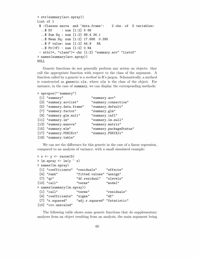
> str(summary(aov.spray))
List of 1
$ :Classes anova and ‘data.frame’: 2 obs. of 5 variables:
..$ Df : num [1:2] 5 66
..$ Sum Sq : num [1:2] 88.4 26.1
..$ Mean Sq: num [1:2] 17.688 0.395
..$ F value: num [1:2] 44.8 NA
..$ Pr(>F) : num [1:2] 0 NA
- attr(*, "class")= chr [1:2] "summary.aov" "listof"
> names(summary(aov.spray))
NULL
Generic functions do not generally perform any action on objects: theycall the appropriate function with respect to the class of the argument. Afunction called by a generic is a method in R’s jargon. Schematically, a methodis constructed as generic.cls , where cls is the class of the object. Forinstance, in the case of summary, we can display the corresponding methods:
> apropos("^summary")
[1] "summary" "summary.aov"
[3] "summary.aovlist" "summary.connection"
[5] "summary.data.frame" "summary.default"
[7] "summary.factor" "summary.glm"
[9] "summary.glm.null" "summary.infl"
[11] "summary.lm" "summary.lm.null"
[13] "summary.manova" "summary.matrix"
[15] "summary.mlm" "summary.packageStatus"
[17] "summary.POSIXct" "summary.POSIXlt"
[19] "summary.table"
We can see the difference for this generic in the case of a linear regression,compared to an analysis of variance, with a small simulated example:
> x <- y <- rnorm(5)
> lm.spray <- lm(y ~ x)
> names(lm.spray)
[1] "coefficients" "residuals" "effects"
[4] "rank" "fitted.values" "assign"
[7] "qr" "df.residual" "xlevels"
[10] "call" "terms" "model"
> names(summary(lm.spray))
[1] "call" "terms" "residuals"
[4] "coefficients" "sigma" "df"
[7] "r.squared" "adj.r.squared" "fstatistic"
[10] "cov.unscaled"
The following table shows some generic functions that do supplementaryanalyses from an object resulting from an analysis, the main argument being
60

this latter object, but in some cases a further argument is necessary like forpredict or update.
add1 tests successively all the terms that can be added to a model
drop1 tests successively all the terms that can be removed from a model
step selects a model with AIC (calls add1 and drop1)
anova computes a table of analysis of variance or deviance for one or severalmodels
predict computes the predicted values for new data from a fitted model
update re-fits a model with a new formula or new data
There are also various utilities functions that extract information from amodel object or a formula, such as alias which finds the linearly dependentterms in a linear model specified by a formula.
Finally, there are, of course, graphical functions such as plot which dis-plays various diagnostics, or termplot (see the above example), though thislatter function is not generic but calls predict.
5.4 Packages
The following table lists the standard packages which are distributed with abase installation of R. Some of them are loaded in memory when R starts; thiscan be displayed with the function search:
> search()
[1] ".GlobalEnv" "package:methods"
[3] "package:stats" "package:graphics"
[5] "package:grDevices" "package:utils"
[7] "package:datasets" "Autoloads"
[9] "package:base"
The other packages may be used after being loaded:
> library(grid)
The list of the functions in a package can be displayed with:
> library(help = grid)
or by browsing the help in html format. The information relative to eachfunction can be accessed as previously seen (p. 7).
61

Package Description
base base R functionsdatasets base R datasetsgrDevices graphics devices for base and grid graphicsgraphics base graphicsgrid grid graphicsmethods definition of methods and classes for R objects and program-
ming toolssplines regression spline functions and classesstats statistical functionsstats4 statistical functions using S4 classestcltk functions to interface R with Tcl/Tk graphical user interface
elementstools tools for package development and administrationutils R utility functions
Many contributed packages add to the list of statistical methods availablein R. They are distributed separately, and must be installed and loaded inR. A complete list of the contributed packages, with descriptions, is on theCRAN Web site18. Several of these packages are recommanded since they coverstatistical methods often used in data analysis. The recommended packagesare often distributed with a base installation of R. They are briefly describedin the following table.
Package Description
boot resampling and bootstraping methodsclass classification methodscluster clustering methodsforeign functions for reading data stored in various formats (S3,
Stata, SAS, Minitab, SPSS, Epi Info)KernSmooth methods for kernel smoothing and density estimation (in-
cluding bivariate kernels)lattice Lattice (Trellis) graphicsMASS contains many functions, tools and data sets from the li-
braries of “Modern Applied Statistics with S” by Venables& Ripley
mgcv generalized additive modelsnlme linear and non-linear mixed-effects modelsnnet neural networks and multinomial log-linear modelsrpart recursive partitioningspatial spatial analyses (“kriging”, spatial covariance, . . . )survival survival analyses
18http://cran.r-project.org/src/contrib/PACKAGES.html
62

There are two other main repositories of R packages: the Omegahat Projectfor Statistical Computing19 which focuses on web-based applications and in-terfaces between softwares and languages, and the Bioconductor Project20
specialized in bioinformatic applications (particularly for the analysis of micro-array data).
The procedure to install a package depends on the operating system andwhether R was installed from the sources or pre-compiled binaries. In thelatter situation, it is recommended to use the pre-compiled packages availableon CRAN’s site. Under Windows, the binary Rgui.exe has a menu “Packages”allowing to install packages via internet from the CRAN Web site, or fromzipped files on the local disk.
If R was compiled, a package can be installed from its sources which aredistributed as a ‘.tar.gz’ file. For instance, if we want to install the package gee,we will first download the file gee 4.13-6.tar.gz (the number 4.13-6 indicatesthe version of the package; generally only one version is available on CRAN).We will then type from the system (and not in R) the command:
R CMD INSTALL gee_4.13-6.tar.gz
There are several useful functions to manage packages such as installed.packages, CRAN.packages, or download.packages. It is also useful to typeregularly the command:
> update.packages()
which checks the versions of the packages installed against those availableon CRAN (this command can be called from the menu “Packages” underWindows). The user can then update the packages with more recent versionsthan those installed on the computer.
19http://www.omegahat.org/R/20http://www.bioconductor.org/
63

6 Programming with R in pratice
Now that we have done an overview of R’s functionalities, let us return to thelanguage and programming. We will see a few simple ideas likely to be usedin practice.
6.1 Loops and vectorization
An advantage of R compared to softwares with pull-down menus is the possibil-ity to program simply a series of analyses which will be executed successively.This is common to any computer language, but R has some particular featureswhich make programming easier for non-specialists.
Like other languages, R has some control structures which are not dissim-ilar to those of the C language. Suppose we have a vector x, and for eachelement of x with the value b, we want to give the value 0 to another variabley, otherwise 1. We first create a vector y of the same length than x:
y <- numeric(length(x))
for (i in 1:length(x)) if (x[i] == b) y[i] <- 0 else y[i] <- 1
Several instructions can be executed if they are placed within braces:
for (i in 1:length(x)) {
y[i] <- 0
...
}
if (x[i] == b) {
y[i] <- 0
...
}
Another possible situation is to execute an instruction as long as a condi-tion is true:
while (myfun > minimum) {
...
}
However, loops and control structures can be avoided in most situationsthanks to a feature of R: vectorization. Vectorization makes loops implicit inexpression, and we have seen many cases. Let us consider the addition of twovectors:
64

> z <- x + y
This addition could be written with a loop, as this is done in most lan-guages:
> z <- numeric(length(x))
> for (i in 1:length(z)) z[i] <- x[i] + y[i]
In this case, it is necessary to create the vector z beforehand because ofthe use of the indexing system. We realize that this explicit loop will workonly if x and y are of the same length: it must be changed if this is not true,whereas the first expression will work in all situations.
The conditional executions (if ... else) can be avoided with the useof the logical indexing; coming back to the above example:
> y[x == b] <- 0
> y[x != b] <- 1
In addition to being simpler, vectorized expressions are computationallymore efficient, particularly with large quantities of data.
There are also several functions of the type ‘apply’ which avoids writingloops. apply acts on the rows and/or columns of a matrix, its syntax isapply(X, MARGIN, FUN, ...), where X is a matrix, MARGIN indicates whetherto consider the rows (1), the columns (2), or both (c(1, 2)), FUN is a function(or an operator, but in this case it must be specified within brackets) to apply,and ... are possible optional arguments for FUN. A simple example follows.
> x <- rnorm(10, -5, 0.1)
> y <- rnorm(10, 5, 2)
> X <- cbind(x, y) # the columns of X keep the names "x" and "y"
> apply(X, 2, mean)
x y
-4.975132 4.932979
> apply(X, 2, sd)
x y
0.0755153 2.1388071
lapply() acts on a list: its syntax is similar to apply and it returns a list.
> forms <- list(y ~ x, y ~ poly(x, 2))
> lapply(forms, lm)
[[1]]
Call:
FUN(formula = X[[1]])
Coefficients:
65

(Intercept) x
31.683 5.377
[[2]]
Call:
FUN(formula = X[[2]])
Coefficients:
(Intercept) poly(x, 2)1 poly(x, 2)2
4.9330 1.2181 -0.6037
sapply() is a flexible variant of lapply() which can take a vector or amatrix as main argument, and returns its results in a more user-friendly form,generally as a table.
6.2 Writing a program in R
Typically, an R program is written in a file saved in ASCII format and namedwith the extension ‘.R’. A typical situation where a program is useful is whenone wants to do the same tasks several times. In our first example, we wantto do the same plot for three different species of birds, the data being in threedistinct files. We will proceed step by step, and see different ways to programthis very simple problem.
First, let us make our program in the most intuitive way by executing suc-cessively the needed commands, taking care to partition the graphical devicebeforehand.
layout(matrix(1:3, 3, 1)) # partition the graphics
data <- read.table("Swal.dat") # read the data
plot(data$V1, data$V2, type="l")
title("swallow") # add a title
data <- read.table("Wren.dat")
plot(data$V1, data$V2, type="l")
title("wren")
data <- read.table("Dunn.dat")
plot(data$V1, data$V2, type="l")
title("dunnock")
The character ‘#’ is used to add comments in a program: R then goes tothe next line.
The problem of this first program is that it may become quite long if wewant to add other species. Moreover, some commands are executed severaltimes, thus they can be grouped together and executed after changing somearguments. The strategy used here is to put these arguments in vectors ofmode character, and then use the indexing to access these different values.
66

layout(matrix(1:3, 3, 1)) # partition the graphics
species <- c("swallow", "wren", "dunnock")
file <- c("Swal.dat" , "Wren.dat", "Dunn.dat")
for(i in 1:length(species)) {
data <- read.table(file[i]) # read the data
plot(data$V1, data$V2, type="l")
title(species[i]) # add a title
}
Note that there are no double quotes around file[i] in read.table()
since this argument is of mode character.Our program is now more compact. It is easier to add other species since
the vectors containing the species and file names are at the beginning of theprogram.
The above programs will work correctly if the data files ‘.dat’ are locatedin the working directory of R, otherwise the user must either change the work-ing directory, or specifiy the path in the program (for example: file <-
"/home/paradis/data/Swal.dat"). If the program is written in the file My-birds.R, it will be called by typing:
> source("Mybirds.R")
Like for any input from a file, it is necessary to give the path to access thefile if it is not in the working directory.
6.3 Writing your own functions
We have seen that most of R’s work is done with functions which argumentsare given within parentheses. Users can write their own functions, and thesewill have exactly the same properties than other functions in R.
Writing your own functions allows an efficient, flexible, and rational use ofR. Let us come back to our example of reading some data followed by plottinga graph. If we want to do this operation in different situations, it may be agood idea to write a function:
myfun <- function(S, F)
{
data <- read.table(F)
plot(data$V1, data$V2, type="l")
title(S)
}
To be executed, this function must be loaded in memory, and this can bedone in several ways. The lines of the function can be typed directly on thekeyboard, like any other command, or copied and pasted from an editor. Ifthe function has been saved in a text file, it can be loaded with source()
67

like another program. If the user wants some functions to be loaded eachtime when R starts, they can be saved in a workspace .RData which will beloaded in memory if it is in the working directory. Another possibility is toconfigure the file ‘.Rprofile’ or ‘Rprofile’ (see ?Startup for details). Finally,it is possible to create a package, but this will not be discussed here (see themanual “Writing R Extensions”).
Once the function is loaded, we will be able with a single command to readthe data and plot the graph, for instance with myfun("swallow", "Swal.dat").Thus, we have now a third version of our program:
layout(matrix(1:3, 3, 1))
myfun("swallow", "Swal.dat")
myfun("wren", "Wrenn.dat")
myfun("dunnock", "Dunn.dat")
We may also use sapply() leading to a fourth version of our program:
layout(matrix(1:3, 3, 1))
species <- c("swallow", "wren", "dunnock")
file <- c("Swal.dat" , "Wren.dat", "Dunn.dat")
sapply(species, myfun, file)
In R, it is not necessary to declare the variables used within a function.When a function is executed, R uses a rule called lexical scoping to decidewhether an object is local to the function, or global. To understand thismechanism, let us consider the very simple function below:
> foo <- function() print(x)
> x <- 1
> foo()
[1] 1
The name x is not used to create an object within foo(), so R will seekin the enclosing environment if there is an object called x, and will print itsvalue (otherwise, a message error is displayed, and the execution is halted).
If x is used as the name of an object within our function, the value of x inthe global environment is not used.
> x <- 1
> foo2 <- function() { x <- 2; print(x) }
> foo2()
[1] 2
> x
[1] 1
This time print() uses the object x that is defined within its environment,that is the environment of foo2.
68

The word “enclosing” above is important. In our two example functions,there are two environments: the global one, and the one of the function foo
or foo2. If there are three or more nested environments, the search for theobjects is made progressively from a given environment to the enclosing one,and so on, up to the global one.
There are two ways to specify arguments to a function: by their positionsor by their names (also called tagged arguments). For example, let us considera function with three arguments:
foo <- function(arg1, arg2, arg3) {...}
foo() can be executed without using the names arg1, . . . , if the corre-sponding objects are placed in the correct position, for instance: foo(x, y,
z). However, the position has no importance if the names of the argumentsare used, e.g. foo(arg3 = z, arg2 = y, arg1 = x). Another feature ofR’s functions is the possibility to use default values in their definition. Forinstance:
foo <- function(arg1, arg2 = 5, arg3 = FALSE) {...}
The commands foo(x), foo(x, 5, FALSE), and foo(x, arg3 = FALSE) willhave exactly the same result. The use of default values in a function definitionis very useful, particularly when used with tagged arguments (i.e. to changeonly one default value such as foo(x, arg3 = TRUE).
To conclude this section, let us see another example which is not purelystatistical, but it illustrates the flexibility of R. Consider we wish to study thebehaviour of a non-linear model: Ricker’s model defined by:
Nt+1 = Nt exp
[
r
(
1 −Nt
K
)]
This model is widely used in population dynamics, particularly of fish. Wewant, using a function, to simulate this model with respect to the growth rater and the initial number in the population N0 (the carrying capacity K isoften taken equal to 1 and this value will be taken as default); the results willbe displayed as a plot of numbers with respect to time. We will add an optionto allow the user to display only the numbers in the last few time steps (bydefault all results will be plotted). The function below can do this numericalanalysis of Ricker’s model.
ricker <- function(nzero, r, K=1, time=100, from=0, to=time)
{
N <- numeric(time+1)
N[1] <- nzero
for (i in 1:time) N[i+1] <- N[i]*exp(r*(1 - N[i]/K))
Time <- 0:time
plot(Time, N, type="l", xlim=c(from, to))
}
69

Try it yourself with:
> layout(matrix(1:3, 3, 1))
> ricker(0.1, 1); title("r = 1")
> ricker(0.1, 2); title("r = 2")
> ricker(0.1, 3); title("r = 3")
70

7 Literature on R
Manuals. Several manuals are distributed with R in R HOME/doc/manual/:
• An Introduction to R [R-intro.pdf],
• R Installation and Administration [R-admin.pdf],
• R Data Import/Export [R-data.pdf],
• Writing R Extensions [R-exts.pdf],
• R Language Definition [R-lang.pdf].
The files may be in different formats (pdf, html, texi, . . . ) depending onthe type of installation.
FAQ. R is also distributed with an FAQ (Frequently Asked Questions) local-ized in the directory R HOME/doc/html/. A version of the R-FAQ isregularly updated on CRAN’s Web site:
http://cran.r-project.org/doc/FAQ/R-FAQ.html
On-line resources. The CRAN Web site hosts several documents, biblio-graphic resources, and links to other sites. There are also a list of publi-cations (books and articles) about R or statistical methods21 and somedocuments and tutorials written by R’s users22.
Mailing lists. There are four discussion lists on R; to subscribe, send a mes-sage, or read the archives see: http://www.R-project.org/mail.html.
The general discussion list ‘r-help’ is an interesting source of informationfor the users of R (the three other lists are dedicated to annoucementsof new versions, and for developers). Many users have sent to ‘r-help’functions or programs which can be found in the archives. If a problemis encountered with R, it is thus important to proceed in the followingorder before sending a message to ‘r-help’:
1. read carefully the on-line help (possibly using the search engine);
2. read the R-FAQ;
3. search the archives of ‘r-help’ at the above address, or by using oneof the search engines developed on some Web sites23;
4. read the “posting guide”24 before sending your question(s).
21http://www.R-project.org/doc/bib/R-publications.html22http://cran.r-project.org/other-docs.html23The addresses of these sites are listed at http://cran.r-project.org/search.html24http://www.r-project.org/posting-guide.html
71

R News. The electronic journal R News aims to fill the gap between theelectronic discussion lists and traditional scientific publications. Thefirst issue was published on January 200125.
Citing R in a publication. Finally, if you mention R in a publication, youmust cite the following reference:
R Development Core Team (2005). R: A language and envi-ronment for statistical computing. R Foundation for Statisti-cal Computing, Vienna, Austria. ISBN 3-900051-07-0, URL:http://www.R-project.org.
25http://cran.r-project.org/doc/Rnews/
72