http://econ.geo.uu.nl/peeg/peeg.html

Papers in Evolutionary Economic Geography

# 09.16

How do regions diversify over time? Industry relatedness and the development of new growth paths in regions

Frank Neffke & Martin Henning & Ron Boschma

1

How do regions diversify over time?

Industry relatedness and the development of new growth paths in regions

Frank Neffke1, Martin Henning2 and Ron Boschma3

16 October 2009

Abstract (242 words)

The question of how new regional growth paths emerge has been raised by many leading

economic geographers. From an evolutionary perspective, there are strong reasons to believe

that regions are most likely to branch into industries that are technologically related to the pre-

existing industries in the region. Employing a new indicator of technological relatedness

between manufacturing industries, we analyze the economic evolution of 70 Swedish regions

during the period 1969-2002 using detailed plant-level data. Our analyses show that the long-

term evolution of the economic landscape in Sweden is subject to strong path dependencies.

Industries that were technologically related to pre-existing industries in a region had a higher

probability to enter the region, as compared to unrelated industries. And unrelated industries

had a higher probability to exit the region. Moreover, we found that industrial profiles of

Swedish regions showed a high degree of technological coherence. Despite substantial

structural change, this coherence was very persistent over time. Our methodology also proved

useful when focusing on the economic evolution of one particular region. Our analysis

showed that the Linköping region increased its industrial coherence during 30 years, due to

1 Erasmus University Rotterdam, The Netherlands (neffke@ese.eur.nl)2 Lund University, Sweden (martin@keg.lu.se)3 Utrecht University, The Netherlands (r.boschma@geo.uu.nl)

2

the entry of industries that were closely related to its regional portfolio on the one hand, and

the exit of industries that were technologically peripheral to its regional portfolio on the other

hand. In sum, we find systematic evidence that the rise and fall of industries is strongly

conditioned by industrial relatedness at the regional level.

Key words: technological relatedness, related variety, regional branching, regional

diversification

JEL codes: R11, N94, O14

3

How do regions diversify over time? Industry relatedness and the development of newgrowth paths in regions

1. Introduction

Regional development is about qualitative change, not quantitative change. Regions are

subject to a never-ending process of creative destruction that Schumpeter (1939) identified as

the driving force behind economic development. That is, in the long run, regions depend on

their ability to create new activities, for example by attracting new local industries, in order to

offset decline and destruction in other parts of their economies. This view inspired economic

geographers in the 1980s to investigate the geographical implications of creative destruction

(e.g. Norton and Rees, 1979; Marshall, 1987; Hall and Preston, 1988). A key finding of that

literature was that newly emerging industries did not necessarily arise in leading regions, but

often triggered growth and development in quite unexpected places, like Silicon Valley in the

US and Bavaria in Germany. Since then, many detailed case studies have investigated both

the success of these new growth regions, and the failure of many old industrial regions to

restructure their economies (see e.g. Scott, 1988; Grabher, 1993). What, however, is still

lacking is a systematic study of how regions diversify over time, how new growth paths in

regions develop, and how old industrial regions revive their local economies (Martin and

Sunley, 2006). In this article, we report on the outcomes of such an inquiry, and we will

demonstrate the pivotal role of technological relatedness in the process of regional

diversification.

The article has three objectives. First, using an evolutionary economic framework, we argue

that technological relatedness is likely to play a crucial role in the diversification processes of

4

regional economies, giving rise to significant path dependencies. Accordingly, we will

explain why regions cannot simply diversify into any new industry, but will rather branch out

into technologically related industries.

Our second objective is to test the empirical validity of this hypothesis of regional branching.

In order to do so, we make use of a recently developed method to accurately quantify

technological relatedness between industries, and we assess whether the entry of new

industries and the exit of existing industries in regions depend on the degree to which these

industries are related to the regional production structure. On the basis of this, on the one

hand, we analyze whether – and if so, quantify the extent to which – local economies in

Sweden can be said to be technological cohesive. On the other hand, we study the processes

of local creative destruction over a period of more than 30 years. That is, we study which

industries enter a region and which industries leave. Comparing this to the extent to which

these industries are related to other industries in the region, we can show that the process of

regional diversification is indeed conditioned by existing regional structures. In particular, we

find that the more technologically related industries are to pre-existing industries in a region,

the more likely they are to enter the region. Similarly, the more peripheral industries are in a

technological sense, the higher the probability that they will leave the region. These analyses

are carried out at a high level of detail, distinguishing between 174 major manufacturing

industries and 70 different labor market regions in Sweden.

The third objective is to investigate how information on industry relatedness can be used as a

tool in case studies of a region to understand its economic evolution. As an example, we take

the Linköping region. Among other things, our analysis highlights how successive exits of

textiles related industries gave rise to a cascading effect that resulted in the loss of an entire

technological cluster of industries in that region.

5

The structure of the article is as follows. In Section 2, we discuss the relationship between

industry relatedness and regional development in an evolutionary framework. In Section 3, we

explain briefly how we constructed our industrial relatedness measure. In Section 4, we

introduce the data. In Section 5, we use this measure to study the development of the

coherence of regional portfolios in Sweden over time. Section 6 studies the role of relatedness

in the Schumpeterian process of creative destruction at the regional level. Section 7 presents

the case study of the Linköping region. Section 8 draws some conclusions and sets out a

future research agenda.

2. Relatedness and the economic evolution of regions

In economic geography, there has been a sustained interest in the question how countries and

regions develop over time. In the 1990s, a rapidly expanding literature started focusing on the

question whether countries and regions converge or diverge over time (see e.g. Barro and

Sala-i-Martin, 1995). At about the same time, the New Economic Geography (NEG) focused

on how globalization and economic integration would affect spatial clustering (Krugman,

1991). Both neo-classical literatures failed, however, to incorporate tendencies of structural

change into their theories and neglected the geographical dimension of creative destruction,

according to which catching-up and falling-behind of countries and regions is analyzed in

terms of the rise and fall of industries (Dosi, 1984; Hohenberg and Lees, 1995).

By contrast, economic geographers embraced Schumpeterian ideas already at an early stage.

In the 1980s, these scholars used spatial versions of the Industry Life Cycle to explain long-

term dynamics in the economic landscape (e.g. Norton, 1979; Markusen, 1985). What they

observed is that regions developing new industries overtook regions that were locked-in in

6

more mature industries. A classic example is the rise of the Sunbelt states in the US, which

left behind the Snowbelt States that were heavily specialized in old and declining industries.

One of the claims of this literature was that old industrial regions with their labor unions, high

wages and crowded streets had fallen victim to their own past industrial success (Storper and

Walker, 1989). By contrast, new growth regions did not suffer from such a legacy, and were

depicted as if they could start from scratch when developing new growth industries. However,

this literature did not give much attention to the question whether already existing regional

industrial structures might boost the emergence and growth of new industries. Nor did it pay

much attention to the possible rebirth or revival of old industrial regions.

At about the same time Krugman published his seminal work, urban economists stumbled

upon the question of structural change through a reappraisal of the works of Jane Jacobs

(1969). Glaeser et al. (1992) extended the agglomeration externalities framework that, until

then, mainly dealt with effects of localization economies and urban size, by investigating the

economic importance of urban diversity. This focus on so-called Jacobs externalities can be

regarded as a first rough attempt to assess the effect of local industrial structure. Henderson et

al. (1995) took a further step in the direction of investigating structural change by studying

whether different types of externalities were important for sustaining mature industries than

for attracting new industries. They found that new (high tech) industries entered diversified

cities where Jacobs’ externalities were available, whereas mature industries benefited more

from the localization externalities generated in more specialized cities (see also Neffke et al.,

2009).

Jacobs’s original reason why new industries needed diversified urban economies was that

urban diversity facilitated a deep division of labour in a city. However, this division of labor

7

contributed to urban growth not so much because of efficiency reasons, as Adam Smith once

argued, but because it gives rise to opportunities for innovation. This fits nicely within the

Schumpeterian framework of innovation as successful new combinations of old ideas. A more

important, but long-neglected implication of Jacobs’ observation was that it abandoned the

image of knowledge as an amorphous quantity, in favour of knowledge as an interconnected

set of qualitatively different ideas. In cognitive theory, such a depiction has led to stress a

trade-off that exists between diversity and similarity: although actors who share a greater

overlap in terms of competences may find it easier to communicate with one another, only

actors that dispose of non-overlapping competences and knowledge can actually offer

something new to be learnt. As a matter of fact, a too strong overlap in competences might

even lead to cognitive lock-in (Nooteboom, 2000).

The notion that in social learning an optimal level of cognitive distance may exist, might

explain why after conducting many empirical studies, evidence on the effects of Jacobs’

externalities is at best inconclusive (e.g. De Groot et al., 2009). Regional knowledge

spillovers will not take place between just any industries, because effective communication is

often hampered by excessive cognitive distance between industries. Recently therefore,

scholars have suggested that industries are more likely to learn from each other when they are

technologically related.4 Accordingly, a wide set of technologically related industries in a

region should be more beneficial than a diversified set of industries, because, by combining

cognitive distance with cognitive proximity, it brings together the positive sides of variety

across and relatedness among industries.

4 In the 1980s, similar ideas had been developed around the notion of technology systems (Carlsson

and Stankiewicz, 1991).

8

Along these lines, Frenken et al. (2007) argue that regions with a higher degree of variety

among related industries in a region, will exhibit more learning opportunities, and

consequently more local knowledge spillovers. The authors show that regions with a high

degree of related variety were indeed associated with the highest employment growth in the

Dutch economy, an effect that was later also found in other countries (Essletzbichler, 2007;

Bishop and Gripaios, 2009). Boschma and Iammarino (2009) have argued that new and

related variety may also flow into a region through inter-industry trade linkages with other

regions. Making use of regional trade data, Boschma and Iammarino found that inflows of

extra-regional knowledge indeed correlated with regional employment growth when these

originated from industries that were related, but not identical, to the industries in the region.

In these studies, the industrial base of a region is treated as a stable property. This makes

sense in the short run, because the industrial composition of a regional economy changes only

slowly on a year-on-year basis. However, it is likely that relatedness among regional

industries not only drives the incremental growth of existing industries through agglomeration

externalities, but may also be responsible for more dramatic shifts in the regional production

structure. In fact, we argue that relatedness of industries may be an important factor in the

attraction of new industries to a region and the disappearance of old ones. This is a

fundamental issue, because it is likely to shed light on how the Schumpeterian process of

creative destruction unfolds at the regional level in the long run. The question of how new

regional growth paths emerge has repeatedly been raised by leading economic geographers in

the past (Scott, 1988; Storper and Walker, 1989) and present (Martin and Sunley, 2006;

Simmie and Carpenter, 2007) as one of the most intriguing and challenging issues in our field.

We expect that the industrial history of regions, and in particular the parts of technology space

9

their portfolios inhabit, will affect the ways regions create new variety over time, and how

they transform and restructure their economies.5

There are many case studies showing that new local industries are often deeply rooted in

related activities in the region (see e.g. Bathelt and Boggs, 2003; Glaeser, 2005). Moreover,

recently, more systematic evidence is becoming available that shows that territories are more

likely to expand and diversify into industries that are closely related to their existing activities

(Hausmann and Klinger, 2007; Hidalgo et al., 2007; Neffke 2009). Focusing on shifts in

export portfolios over time, Hausmann and Klinger (2007) showed that countries

predominantly expanded their export mix by moving into products that were related to their

current export basket, implying that a country’s position in the product space affected its

opportunities for diversification. As a consequence, rich countries which specialised in more

densely connected parts of the product space had more opportunities to sustain economic

growth than poorer countries.

Boschma and Frenken (2009) have termed the process by which new variety (industries)

arises from technologically related industries “regional branching”. The reason this regional

branching process occurs is that new industries can connect to existing industries through

various knowledge transfer mechanisms, and this is likely to support their emergence and

growth. These mechanisms are: (1) firm diversification; (2) entrepreneurship in the form of

spinoffs; (3) labour mobility; and (4) social networking. Since these mechanisms operate

mainly (though not exclusively) at the regional level (i.e. at the sub-national level within

5 This is not to deny that there are other ways to diversify regional economies than through related

diversification. For instance, new industries may enter a region as a result of foreign direct

investments in unrelated industries. In this paper, we concentrate however on how relatedness and

related variety affect the process of regional diversification.

10

regions, rather than between regions), this branching process is essentially a regional

phenomenon. Below, we discuss each of these mechanisms more in detail.

In their diversification strategies, firms tend to build on their existing competences, which

have proven successful in the past. The reason for this is that, as argued by Nelson and Winter

(1982), intra-firm diversification is not without problems, because firms that search for new

markets and new technologies face fundamental uncertainties. Firms try to limit this

uncertainty and avoid major switching costs by conducting search processes that are local in a

technological sense, that is, directed to technologies and markets that are similar to the ones

with which firms have become familiar in the past. Similarly, Penrose (1959) conceived firm

growth as a progressive process of related diversification, in which firms diversify into

products that are technologically related to their current products. This view is corroborated

by the fact that mergers and acquisitions (M&A’s) show higher levels of performance when

they connect firms with technologically related knowledge bases (see e.g. Piscitello, 2004;

Cassiman et al., 2005). Particularly interesting in terms of our earlier discussion on optimal

cognitive distance is Ahuja and Katika’s (2001) finding that neither very high nor very low

levels of overlap, but only a moderate level of overlap between the knowledge bases of the

acquired and the acquiring firm had a positive effect on the subsequent innovation output of

the acquiring firm. Moreover, since new divisions of firms are frequently established inside

existing plants, internal diversification of firms is often not only local in cognitive terms but

also in geographical terms. Similarly, as studies have demonstrated that geographical

proximity is a key determinant of M&A’s within countries (see e.g. Rodriguez-Pose and

Zademach, 2003), external related diversification may also have a geographical bias. In sum,

there are good reasons why related diversification at the firm level (both through internal and

11

external growth) is expected to have a geographical bias, although systematic empirical

evidence is still lacking.

Regional branching through entrepreneurship, in contrast, is already well documented. This

occurs when new firms in a newly emerging industry are set up by entrepreneurs who

previously acquired knowledge and experience in a related industry in the same region. Many

of such experienced entrepreneurs tend to locate near their parents. Moreover, there is

considerable evidence that these firms benefit economically from the experience acquired by

the entrepreneurs in related industries, as reflected in their higher probabilities to survive

(Klepper, 2007). Longitudinal studies have confirmed that these experienced entrepreneurs,

and not so much intra-industry spinoff companies, play a crucial role in the process of

regional branching. Boschma and Wenting (2007) have shown that in the early development

stage of the UK automobile industry, firms had a higher survival rate when their entrepreneurs

had previously worked in related industries like bicycle making, coach making or mechanical

engineering, and when their regions featured a strong presence of these related industries.

Regional branching through labour mobility is yet to be explored. Labour mobility is often

regarded as a key mechanism through which knowledge diffuses (see e.g. Almeida and Kogut

1999; Heuermann 2009), but no attention has been paid to spillovers between firms of related

industries with respect to labour mobility until recently. Boschma et al. (2009) have provided

empirical evidence that the economic effects of inflows of labour cannot be properly assessed

without paying attention to how these knowledge flows are related to the existing knowledge

bases in firms. They found evidence that the inflow of employees with skills that were related

to the knowledge base of the plant was positively related with productivity growth, while the

12

relation with hiring new employees with skills already available in the plant was negative.

However, the role of labour mobility in the constitutive stages of an industry remains to be

studied. If labour mobility indeed induces industrial branching, this is expected to be mainly a

regional phenomenon again, because most employees that change jobs remain in the same

region.

Social networks may be another source of regional branching. Social networks are considered

a major channel of knowledge diffusion and learning among firms (see e.g. Powell et al.,

1996; Sorenson, et al. 2006; Ter Wal, 2009). However, the extent to which networks will

matter for exploration and radical innovations, and thus for developing new economic

activity, may depend on the degree of technological relatedness among the network partners.

Again, in order to stimulate new ideas, while at the same time enabling effective

communication, it is likely that an optimal level of cognitive proximity between network

partners exists (Boschma and Frenken, 2009). Studies on inter-firm alliances networks show

that more radically new knowledge is developed when actors bring in different but related

competences (see e.g. Gilsing et al., 2007). However, also the role networks play in

generating industrial branching has not yet been studied. If they would indeed matter in

connecting old and new industries, we expect they will further contribute to the process of

regional branching, because social networks tend to be highly localized (Breschi and Lissoni,

2003).

The implications of all the above are not to be underestimated. First, the way the

Schumpeterian process of creative destruction shapes the economic landscape should be

affected by industry relatedness at the regional level, as the relatedness among industries

13

would have an impact on which new industries enter and which existing industries will leave

a region. Second, the rise and fall of industries are conditioned by regional industrial

structures laid down in the past, which would support the notion of regional path dependency,

according to which each region follows its own industrial trajectory (Rigby and

Essletzbichler, 1997). Third, this path dependent process implies there is some degree of

coherence in the industrial profile of a region. However, this coherence is constantly being

redefined through the process of creative destruction. Entry of new industries in a region,

although technologically related to existing local industries, is likely to inject new variety into

the region, and will lower technological coherence. In contrast, exits of existing industries

will increase the industrial coherence of regions, because unrelated industries are more likely

to be selected out, leading to a decrease in variety. We will test these ideas empirically to

determine whether, and to what extent, regional industrial structures can be said to be

coherent on the one hand, and how this coherence evolves through the creation of new

industries and destruction of existing industries on the other hand.

3. Measuring relatedness: the revealed relatedness method

In empirical work, inter-industry technological relatedness is often derived from the

hierarchical structure of the standard industrial classification (SIC) system. The closer

industries are within this classification system, the more related they are thought to be.

However, one can question whether SIC-based relatedness measures are truly technological

relatedness measures. As a response to the perceived shortcomings of SIC based relatedness,

industry relatedness measures have for instance been based on similarities in upward and

downward linkages in input-output tables (Fan and Lang 2000), or on similarities in the mix

of occupations employed by different industries (Farjoun 1994). More recently, a number of

scholars have turned to co-occurrence analysis to assess inter-industry relatedness (Teece et

14

al. 1994; Hidalgo et al. 2007; Bryce and Winter 2006). Co-occurrence analysis measures the

relatedness between two industries by assessing whether two industries are often found

together in one and the same economic entity. Hidalgo et al. (2007) count the number of times

that two industries have a revealed comparative advantage (the co-occurrence) in one and the

same country (the economic entity).6 Similarly, Teece et al. (1994) and Bryce and Winter

(2006) count the number of times one firm (the economic entity) owns plants in two different

industries (the co-occurrence). But other factors than relatedness may partly determine the

number of co-occurrences. For example, if industries are very large, they are likely to be

found in many firms, and therefore they will also co-occur with other industries more

frequently. To determine whether the number of co-occurrences between two industries are in

some way excessive, co-occurrences are compared to an (“expected”) baseline. The more

often two industries co-occur relative to this baseline, the higher their score on relatedness.

In this article, we use a co-occurrence based measure to estimate relatedness, called revealed

relatedness (RR) developed by Neffke and Svensson Henning (2008). Industry relatedness is

here derived from the co-occurrence of products that belong to different industries in the

portfolios of manufacturing plants. In essence, the RR index measures the revealed existence

of economies of scope between industries. Note, though, that the RR version that we use here

is derived from product portfolios of plants, not from firm portfolios as in Teece et al. (1994)

and Bryce and Winter (2006). The difference between firm and plant level is crucial, because

the set of economies of scope that matter at the plant level is more restricted than the set of

economies of scope that matter at the firm level. If products from two industries are often

found to be produced in one and the same plant, this is likely to happen because the

production processes in these industries generate economies of scope for one another. For

6 These authors assess relatedness among product categories. Product categories can however fairly

easily be translated into industrial categories.

15

instance, the same machinery may be used in both industries, or both industries require

employees with similar skills. In contrast, if economies of scope between two industries are

absent, it is unlikely that firms will combine the different production processes in one plant.

As an illustration, the sportswear firm Nike uses its strong firm brand name to diversify from

its sports clothing line into sports watches. No doubt watch making and sports apparel

manufacture are unrelated in a technological sense. It is, however, also unlikely that Nike’s

shirts and watches are produced in the same plants. The plant level relatedness estimates in

Neffke and Svensson Henning’s index will, therefore, predominantly reflect the degree of

technological relatedness among industries.

The construction of the revealed relatedness (RR) index involves three steps. In the first step,

the number of co-occurrences between the industries is determined for each combination of

two industries ( , ).7 Let us this denote the number of co-occurrences by . But the number

of co-occurrences does not only depend on the relatedness among industries. For instance,

firms are more likely to add highly profitable industries to their portfolios than industries with

low profitability. Regardless of their relatedness to other industries, the probability of

encountering a large industry in a co-occurrence is bigger than the probability of encountering

a small industry.

In the second step, the RR method in Neffke and Svensson Henning control for such effects

by determining the number of co-occurrences for a combination ( , ) that would be expected

on the basis of such industry level characteristics alone. We run a regression of the observed

co-occurrences on the overall profitability, employment and number of active plants in

both industries. Using the estimated parameters it is possible to calculate predictions of the

7 Because the precision of the estimates in symmetric RR matrices is higher, we only use symmetric

relatedness in this article (see Neffke and Svensson Henning 2008).

16

number of co-occurrences, , for each combination of industries ( , ). For instance, in our

data the predicted “baseline” number of co-occurrences between industries 382200

(manufacture of agricultural machinery and equipment) and 384320 (manufacture of motor

vehicles engines, parts and trailers) in 1980 based on profitability, number of employees and

number of plants in both industries, is be 4.99. This prediction is then compared to the

observed number of co-occurrences, which for the example above was 36. The observed

number of co-occurrences exceeds in this case expectations by a factor of 7.21, which

indicates that the industries are strongly related to one another. In the third step, this factor is

multiplied with a constant to arrive at an index that for all industry combinations lies between

0 and 1.8 The basic estimate of RR can be written as:

(1) =

where is the normalizing constant. For 1980, this constant equals to . . Consequently, the

relatedness between the agricultural machinery industry and the motor vehicles industry is

0.59.

For most industry combinations, this procedure suffices to construct an accurate relatedness

measure. However, some industries are so small that a difference of one co-occurrence results

in dramatic changes in the RR estimate. For these cases, additional indirect information that

can be found in the overall matrix of the relatedness estimates is used. The main insight that is

8 The normalizing procedure does not substantially change the index, but only redefines the units in

which it is measured. The reason the authors normalize the index is that in order to be able to enhance

the quality of relatedness estimates using indirect information, relatedness values must be restricted to

the interval [0,1]. Details can be found in Neffke and Svensson Henning (2008).

17

used is the fact that if an industry is related to both industry and industry , then industry

and are likely to be related to one another as well. The exact details of how this indirect

information can be merged with the direct co-occurrence information by means of Bayesian

inference can be found in Neffke and Svensson Henning (2008).

4. Data

For the empirical applications, we use two datasets which were obtained from Statistics

Sweden. The dataset used to estimate industry relatedness contains information about the

products produced in Swedish manufacturing plants in the period from 1969 to 2002. The

products were first translated into standard industry (SNI69) codes and were then used to

define the plants’ portfolios. For example, if a plant produces two different products, say a

and b, and these products are classified as belonging to industries and , this counts as a co-

occurrence between the industries and . Although the number of registered plants in the

database decreases over time due to changing sampling regimes and the shift of the economy

out of manufacturing and into services, we still have information on the production structure

of some 2,000 plants even in the last year of 2002.

In order to determine which industries are active in each of the 70 Swedish regions, we

aggregate a dataset containing plant level employment and industry affiliation information to

the regional level. The original dataset includes all manufacturing plants in Sweden with five

or more employees for the period 1969-1989, and plants with over five employees that belong

to firms with at least ten employees for the period 1990-2002. Unlike the product portfolio

data, each plant in this database has only one industry affiliation (which corresponds to its

main activity). Therefore, the fact that two industries co-occur in one plant in the product

portfolio database, does not imply that both industries are also both found in the region where

18

the plant is located. For two industries to be present in the same region, each needs to have at

least one plant in the region with a main activity that belongs to the particular industry. Thus,

plant level co-occurrence does not automatically imply co-occurrence at the regional level.

5. Relatedness and structural change in regions

Using these product portfolio datasets, we can estimate a matrix of RR indices that covers 174

6-digit industries in the Swedish manufacturing sector.9 Figure 1 visualizes this matrix by

depicting industry space, a network graph connecting related industries. Each node in the

graph represents a 6-digit industry, and the different colors and symbols reflect the various 2-

digit SNI69 categories they belong to. Lines that connect the industries represent RR linkages.

The arrangement of industries in this picture is such that more related industries are located

more closely together in the two dimensional plane.10 As a result, industry space can be used

to get an impression of which industries are relatively closely related to each other.

-­‐ Figure 1 about here –

9 We calculate a RR matrix for each year in the period 1969-2002. In principle, RR can change,

reflecting dynamics in the technological distances between industries. The general relatedness

structure of the economy is, however, fairly stable, although there are also some shifts visible in these

30 years of economic development. Investigating the consequences of treating relatedness as a

dynamic concept is, however, left for future research. In the analysis below, we use average

relatedness indices over time to arrive at a single RR matrix.10 We use the spring embedded algorithm of the NetDraw software (Borgatti 2002). Only the 2,500

strongest links are displayed.

19

A striking feature of the graph in Figure 1 is that industries are located in clearly

distinguishable sets of related industries. We refer to these sets of industries that are close to

each other in industry space as “technological clusters”. This should not be confused with the

term “geographical clusters” which refers to the phenomenon of spatial clustering of

industries. To some extent, technological clusters follow the hierarchical structure of the 2-

digit SNI-codes. For example, machinery industries (light blue upward triangles), textiles

industries (dark blue diamonds), food industries (red circles), et cetera all cluster together in

industry space. Yet, there are also many exceptions: some steel and metal industries (light

green diamonds) are closely located to the machinery cluster and the concrete industry is

more closely located to the chemicals cluster than to many of its fellow mineral products

industries (dark green circles in black boxes). In fact, SNI-relatedness as defined by the

proximity between two industries in the SNI69 hierarchy correlates for 38%11 with our RR

index. This shows that although industry space does to a certain degree correspond to the

SNI69 hierarchy, it by no means completely coincides with it. Moreover, unlike the SNI69

hierarchy, industry space also shows how different technological clusters of related industries

are positioned relatively to each other. For example, the textiles industries are more closely

related to many machinery and metal industries than to most food industries. This confirms

the intuition that spillover potentials between machinery and textiles industries should be

greater than between textiles and food industries.

Because our aim is to investigate whether the process of creative destruction is affected by

industrial relatedness at the regional level, we first examine the magnitude of this regional

structural change. Figure 2 shows the dynamics of Swedish local industries over the entire

time period. For the period from 1969 to 2002, Swedish regions underwent substantial

11 This number represents the rank correlation between the off-diagonal elements of the RR matrix

with the corresponding SNI-relatedness.

20

structural change. If we look at the local industries, i.e., industry-region combinations, that

existed in the whole of Sweden in 1969, only 55.0 % still exist in 2002. Turning the

perspective around, 68.7 % of all local industries in 2002 already existed in 1969.

-­‐ Figure 2 about here -­‐

In previous sections, we argued that such processes of structural change in regional

economies are expected to follow a distinctly evolutionary logic of industrial branching and

path dependence. Accordingly, new economic activities will not be developed in just any

industry, but they will rather be a part of industries that are technologically related to the

present industries in a region.

In order to investigate this issue, it is insufficient just to know how related a particular

industry is to another industry. What we need is a definition of what it means that an industry

is technologically close to a complete portfolio of industries. We propose to use an index that

counts the number of industries in region ’s portfolio that are more closely related to industry

than a threshold value.12 Keeping in mind that all RR values lie between 0 and 1 we choose

this threshold to be 0.25, but results are very similar for a wide range of threshold values. If

(. ) is an indicator function that takes the value 1 if its argument is true and 0 if its argument

is false, can be defined as:

12 We have also experimented with an index that calculates the distance of an industry to the

technological envelope of a region. That is, we calculated the distance between the industry and the

closest industry that was a member of the regional portfolio. The results presented below are similar to

the ones we get when using this alternative measure.

21

(2) = > 0.25( )

Figure 3 illustrates this calculation. We have plotted a regional portfolio in this graph by

coloring all local industries of the region blue. Lines that connect two nodes indicate that the

two industries are related, which we here take to mean that the relatedness between them is at

least 0.25. For instance, industry 3, which is part of the regional portfolio, is related to

industries 1, 2, 5 and 6. Industries 1, 2 and 6 are part of the regional portfolio. As in total there

are three industries that exhibit a relatedness of at least 0.25 to industry 3, the closeness of

industry 3 to the regional portfolio is 3. Similarly, we can see that the closeness of industry

20, which is absent in this particular region, is equal to 2.

-­‐ Figure 3 about here -

The average of the closeness values across all industries that are present in a regional portfolio

can be regarded as a quantification of the technological cohesion of a regional economy:

\

(3) =

For instance, in the situation of Figure 3, the technological cohesion of the depicted region

equals (3 + 3 + 3 + 2 + 2 + 1 + 0 + 2 + 1 + 1) 10/ = 1.8.

22

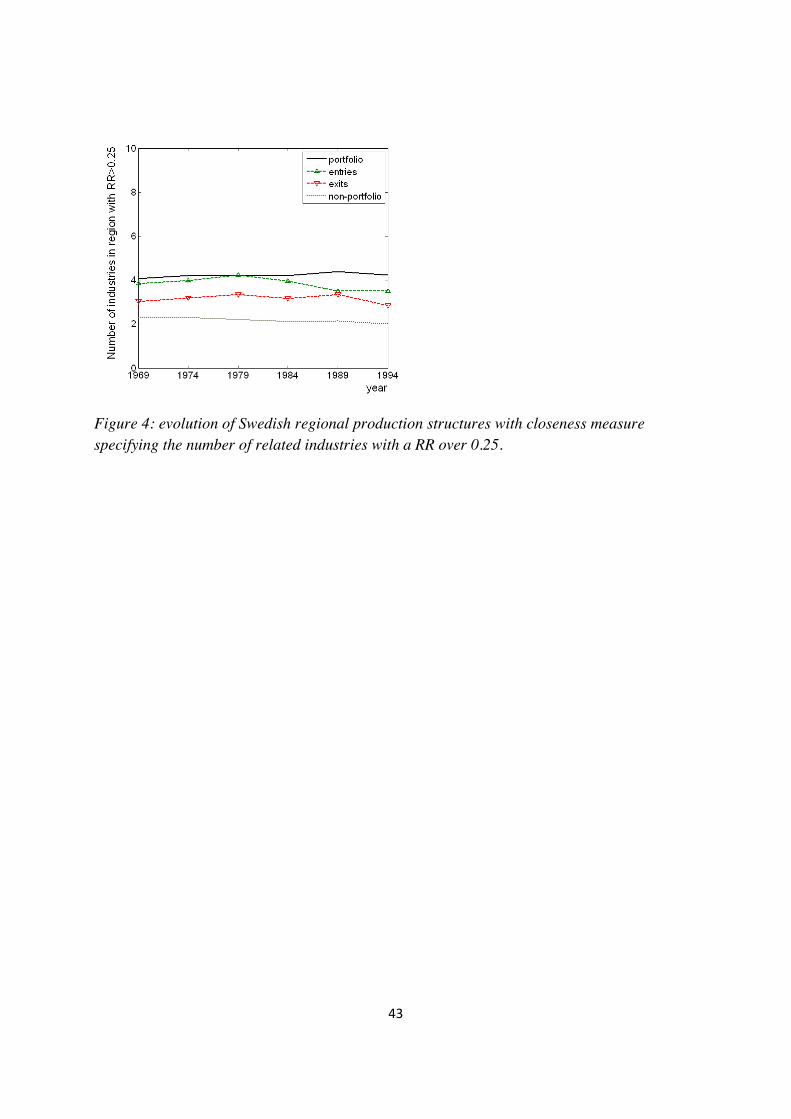
Figure 4 describes the evolution of the average technological cohesion across all Swedish

regions. The solid line in this figure depicts the closeness of industries to their regional

portfolios, averaged across the whole of Sweden at a five-year interval. The dotted line

depicts the average closeness of all industries in the portfolio to the industries that are not a

part of the regional portfolio. This provides us with a baseline against which we can compare

technological cohesiveness. We will say that a regional portfolio is cohesive if its members

are closer to each other than to industries that do not belong to the regional portfolio (that is,

regions are cohesive if the solid line lies above the dotted line). In Figure 4, this is clearly the

case for all years.

-­‐ Figure 4 about here -­‐

Although cohesion of relatedness seems to be a stable phenomenon over time, the graphs

might obscure a substantial amount of structural change as new industries enter and existing

industries exit regions. Therefore, for all industries that exit or enter a region within a five-

year window, we plotted their average closeness to the corresponding regional portfolios. The

line with the upward triangles denotes the closeness of entering industries to the portfolio. The

line with the downward triangles denotes the closeness of exiting industries to the portfolio.

The line that represents entries is always above the (dotted) non-portfolio line. This means

that the industries that enter a region are strikingly closer to the region’s portfolio, than the

industries that remain outside this portfolio. Or, to turn things around, regions indeed

diversify into industries that are related to their current portfolios of industries. Remarkably,

not only the line representing entries, but also the line that represents exits lies above the grey

23

(non-portfolio line). This is in fact not that surprising: we already saw that regional portfolios

are in general cohesive, meaning that industries that were former members were probably not

completely unrelated to the other economic activities in the region. However, the exits-line is

always well below the (solid) portfolio line. That is, although these exiting industries were not

unrelated to the other local industries, on average, their technologically position vis-à-vis the

regional portfolio was rather peripheral.

Upon closer inspection of the entry-line, entries turn out to be generally not more closely

related to the portfolio than existing portfolio members are. If anything, the entry line is below

the portfolio line and entrants should decrease the technological cohesion of a portfolio.13

This is in line with the evolutionary notion of mutations, according to which new activities

increase the variety in a population. As the exit line is well below the portfolio line, exits, on

the other hand, should increase the average cohesion of a region, analogously to the variation

reducing effect of natural selection. The net effect of mutations and selection is a coherence

that seems to be remarkably stable over time.

In sum, we find three different regularities that relate to our research questions. The first is

that regional production portfolios are cohesive, and remain so over time. As a corollary one

would expect that, if an industry is technologically close to a regional portfolio chances are

high that it is actually a part of that portfolio. The second is that industries that do not belong

to a regional portfolio are more likely to enter portfolios they are technologically close to. The

13 In practice, however, entering industries with a closeness to the portfolio members that is lower than

the closeness among the portfolio members themselves can lead to a higher overall cohesion. This

happens whenever an industry fills a “gap” in the region’s portfolio and takes a central position among

a number of otherwise rather disparate portfolio members. Because of this bridging feature, these

entries might have a huge effect on regional development, comparable to filling a structural hole in

network theory.

24

third regularity is that industries that belong to a portfolio, but are at its technological

periphery, are more likely to leave the region. In the next section, we examine these results

further.

6. Portfolio membership, entry, and exit

Let us start by defining dummy variables for membership, entry and exit in the industrial

portfolio of a region. The membership dummy takes on the value 1 if an industry is part of

the industrial portfolio of region at time . The entry dummy takes on the value 1 if an

industry does not belong to the industrial portfolio of region at time , but enters this

portfolio by time + 5. The exit dummy takes on the value 1 if an industry is part of the

industrial portfolio of region at time , but leaves the region by time + 5. Formally:

(4) = ( , )

(5) = ( , ) ( , + 5)

(6) = ( , ) ( , + 5)

Table 1 shows the correlations between these dummies and closeness to the regional

portfolios if we pool data on all 70 regions and all 5-year periods between 1969 and 2002.

Obviously, in order to be able to enter a portfolio an industry first has to be absent from the

regional portfolio and an industry can only exit the region if before it used to be a part of the

regional portfolio. In the table, we have restricted the samples for the correlations with entry

and exit dummies accordingly.

25

-­‐ Table 1 about here -­‐

As expected, entry and membership are both positively correlated and exit is negatively

correlated with both closeness measures. Although the correlations may not strike one as

particularly high, they are strongly significant in a statistical sense. To find out whether the

impact of closeness variables on regional portfolios is also economically significant, we

analyze how these variables affect entry, exit and membership probabilities. In the five-yearly

sample, summed across all years and all time periods, there are 2,766 events of an industry

entering a region. An industry can only enter a certain region in a given period if it did not yet

belong to the region’s portfolio at the beginning of the period. In total there were 52,226 such

entry opportunities. That is, summed across all time periods, there were 52,226 industry-

region combinations for which the industries did not belong to the portfolio of the

corresponding region. As a result, we can estimate the entry probability to be

2,766/52,226=5.3%. Similarly, the overall exit probability was 16.6%, since there were 3,464

events of an industry leaving a region and 20,854 exit opportunities. Finally, membership

probability is estimated to be 28.5% (20,854 out of all 73,080 possible regional industries

existed). Each industry-region combination can be attributed to a specific closeness value

using the method depicted in Figure 3. If we separately calculate the membership, entry, and

exit probabilities for each value the closeness variable can assume, we can plot how these

probabilities change as closeness increases (Figures 5 to 7).

-­‐ Figures 5-­‐7 about here –

26

When moving along the closeness-axis, we see that both membership and entry probabilities

are at first well below their overall average values but end far above them. Membership

probabilities increase by a factor 4.5 when comparing values at closeness of 0 to values at

closeness over 10. Entry probabilities rise even sevenfold. By contrast, exit probabilities start

at 25%, but drop to below a third of that value. These numbers show that the effect of

closeness on portfolio dynamics is not only statistically significant, but also has substantial

economic implications.

To control for possible confounding variables in our analyses, we run a number of regression

analyses. Tables 2-4 show the outcomes.

-­‐ Tables 2-­‐4 about here -­‐

The first three columns of Tables 2-4 contain the outcomes of the regression of membership,

exit and entry dummies on an industry’s closeness to the portfolio of a region and a constant.

The samples have been restricted in the same way as in Table 1. Below the parameter

estimates, we report robust standard errors.

The first column contains a linear probability model, which is simply an OLS of the dummy

variables on the regressors. Again all estimates are as we would expect. An industry’s

closeness the regional portfolio increases the probability that it is already a member of the

regional portfolio, or, if it is not yet a member, that it will enter the region within a five year

period. As shown by the negative coefficient in Table 4, the probability that an industry leaves

a region drops with the number of industries to which it is closely related. The attractive

feature of the OLS model is that the numeric interpretation of the estimates is immediately

27

clear. For example, if we let the closeness value increase from 0 to 10, the membership

probability rises from 18.1% to 56.1%, the entry probability rises from 2.7% to 14.7%, and

the exit probability drops from 20.8% to 10.8%. These values are very close to the values we

find in Figures 5-7. OLS is however not an appropriate estimation technique for binary

variables. Therefore, we also estimate probit and logit models. Coefficients of these models

are not readily comparable.14 However, the signs and significance levels of the parameters in

both columns confirm the earlier findings of the OLS estimations.

The membership, entry and exit dummies are likely to be affected by the overall size of both

the industry and of the region. After all, large industries will more often be a member of a

regional portfolio, and they are more likely to enter and less likely to completely exit a region.

Similarly, large regions will host a large number of different industries, and are able to attract

new and retain old industries more easily. To control for such effects, column (4) adds two

new variables, log(emp( )) and log(emp( )), which measure the log of total manufacturing

employment in region and of total Swedish employment in industry respectively. In order

to get a rough notion of the size of the effects, we also estimate an OLS model in column (5).

Both variables have the expected effects in all three tables, but adding these variables

substantially reduces the size of estimated coefficients. Yet, the influence of closeness

remains strongly significant for membership, entry and exit probabilities alike.

14 The coefficients of probit and logit models are in general difficult to compare, as estimated effects

change with changes in the regressor values. One way to compare parameter estimates across these

models is by evaluating the marginal effects at the mean of the closeness variable. The estimates for

membership regressions of probit and logit models are fairly similar at 0.0412 and 0.0355

respectively, with the OLS estimate in between. The exit estimates are similarly comparable at,

-0.0184 and -0.0117, but are somewhat higher than the OLS estimates. The biggest difference is found

in the estimates of average marginal effects on entry, where the probit model gives a value of 0.033

and the logit of 0.0075.

28

In columns (6) and (7), we add a final variable, closeness(non-PF). Again, the OLS estimates

in column (7) should only be taken as indicative. Whereas the closeness(PF) variable

measures the closeness of an industry to a region’s portfolio, this variable measures the

closeness of an industry to all industries that are absent from the region’s portfolio. In other

words, we assess what happens when an industry has to get by without the local presence of a

number of industries to which it is strongly related. Table 2 shows that the effect on

membership probabilities is substantial. If industry is strongly related to industries that are

absent from region , this industry is likely to be also itself absent from this region. Table 3

shows that such missing related industries also lead to lower entry rates. Table 4 completes

this picture by showing that the absence of a large number of related industries may lead

industries to leave, even though there may still be many related industries left in the region. In

fact, this could initiate a domino effect, where the departure of a small number of industries

may lead to a complete dismantling of a larger technological cluster in the region. In the next

section, we will take a closer look at the region of Linköping where after such a domino effect

the entire local cluster of textiles industries had abandoned the region.

To summarize, the regression analyses confirm the three regularities that we identified in the

previous section. The closeness of an industry to a regional portfolio has important

consequences for the technological cohesion of a region – in terms of membership

probabilities – and for the evolution of its industrial structure, both in terms of entering and of

exiting industries.

7. Industrial transformation in the Linköping region: a case study

The RR index and industry space can be used as supporting tools when trying to make sense

of the complex long-run structural dynamics of individual regions. In this section, we

29

illustrate this using the Linköping region in the southern part of Sweden. To give a general

picture, the region is of medium sized with a number of inhabitants that increased from

85,000 in 1970 to 101,000 in 2000. Historically, Linköping is primarily known for its

specialization in machinery and aviation technology, but more recently, the region has also

become home to a number of more high-tech industries, such as IT. In terms of educational

endowments, Linköping houses a major university.

To study the structural evolution of the region, Figure 8 shows Linköping’s manufacturing

portfolio in industry space, and the changes it underwent between 1970 and 2000. The grey

circles symbolize industries that are neither found in Linköping in 1970, nor in 2000. The blue

circles represent industries that are present both in 1970 and in 2000. The upward pointing,

green triangles represent industries that are present in Linköping in 2000, but not in 1970. The

darker the shading of green, the earlier the industry entered the region. Similarly, the red,

downward pointing triangles indicate industries that were found in Linköping in 1970, but

that had left the region by 2000. Again, darker colors indicate that the exits took place earlier.

The picture clearly highlights Linköping’s strong presence in metal and machinery industries.

-­‐ Figure 8 about here -­‐

Figure 9 shows that the industrial profile of Linköping exhibits a strong degree of

technological coherence. Figure 9 is the regional counterpart to figure 4. It plots the coherence

of Linköping’s portfolio (solid line), its average closeness to the industries outside the own

regional portfolio (dotted line), the average closeness of entering industries (upward pointing

triangles) and of its exiting industries (downward pointing triangles) to Linköping’s portfolio.

30

The portfolio line is always above the non-portfolio line, confirming the coherence that was

suggested by the clustering of industries in Figure 8. However, unlike the situation for

Sweden as a whole, Linköping increases its coherence over time. This increase is fuelled not

only by the exit of industries that are more or less technologically peripheral to its portfolio,

but also, especially in the 1970s, by the entry of industries that are very closely related to the

regional portfolio.

-­‐ Figure 9 about here -­‐

In the industry space of Figure 8, we can see how this evolution took place. The overall

impression is that industries that leave the region (downward triangles) were in general not

supported by a strong technological cluster of related industries in the region. This is the case

for concrete, earthenware, petroleum, medicines, fur, wooden furniture and a range of textiles

industries. Turning to the latter cluster around textiles and a number of wood industries in the

upper left corner, we see that these industries tend to disappear slowly over time. The cluster

was hit hardest in the 1970s, when several industries (carpets, wooden furniture (1), sewing,

shirts and other textiles) left the region. The other industries in the cluster then became very

peripheral to the region’s remaining portfolio. It is therefore not surprising to see fur (1) leave

the region in the 1980s, followed by wood products and paper containers in the 1990s. By the

year 2000, the region had all but lost its complete cluster of textiles and wood industries. This

illustrates how the earlier described domino effects can force industries to leave a region that

at first were not at all peripheral, but made up a strong regional cluster.

31

8. Conclusions

In this article, we studied structural change in industrial portfolios of Swedish regions from an

evolutionary economic perspective. In line with evolutionary reasoning, regional

diversification emerges as a strongly path dependent process. Regions diversify by branching

into industries that are related to their current industries. In particular, industries are more

likely to enter a region if they are technologically close to the regional portfolio. However, in

general, industries that enter a region are less related to the local industrial portfolio than the

average technological proximity among existing portfolio members. Consequently, entry

typically lowers a region’s technological coherence by adding new variety. In this sense, it

fulfils an analogous role to evolutionary mutations. Exit probabilities, in contrast, increase as

industries hold technologically more peripheral positions in a region’s portfolio. Exit thus

increases the technological coherence of regions, which conforms to the variety reducing

effect of selection. However, industries are also more likely to leave if technologically related

industries are missing in the region. As a consequence, the exit of one industry can set a

cascading sequence of exits into motion, leading to the departure of complete technological

clusters. An example of such domino effects was observed in the Linköping region, which,

one by one, lost its entire textiles cluster.

Revealed relatedness and industry space also offer powerful tools for case study analysis and

regional policy making. By depicting a regional portfolio in industry space, policy makers

may identify future threats and opportunities for the region. In particular, our analyses suggest

that it is very difficult to attract new industries to a region if these are technologically distant

from present local activities. Moreover, even if they can be persuaded to enter, the high exit

probabilities of technologically peripheral industries suggest that they will often not last very

32

long. Regional policy should therefore focus on the support of industries that are

technologically related to the existing industries in the region. If new activities are at least

somewhat related to existing activities, stimulating knowledge transfer mechanisms (like

entrepreneurship, labour mobility and networking) has a better chance of effectively

embedding these new industries in regional production structures.

In terms of future research, the relatedness perspective opens up a whole new research

agenda. First, the systematic evidence presented here shows that new growth paths in regions

do not start from scratch but are strongly rooted in the historical economic structure of a

region. This could be an interesting perspective for the study of the rise of spatial clusters,

which currently draws much attention (see e.g. Menzel and Fornahl, 2009). It could also help

us understand better how old industrial regions restructure and adjust their economies over

time. Especially in the context of the current economic crisis, this topic of regional resilience

ranks highly on the scientific and political agenda. Second, there is a strong need to determine

through which mechanisms the process of regional branching operates. In Section 2, we

mentioned four candidates (i.e. firm diversification, entrepreneurship, labour mobility and

networking). However, their importance in the development of new regional growth paths still

needs to be explored (Boschma and Frenken, 2009). Third, we need more in-depth analysis of

the implications of the entry of new industries that bridge two technology clusters in a region.

Although it is plausible that these industries have a large impact on long-term regional

development, so far empirical evidence is lacking. Fourth, our study has focused on regional

portfolios, to the neglect of inter-regional effects. Spillovers between related industries are

probably not restricted to a region, but will also be manifest between neighboring or highly-

connected regions. Fifth, when examining how technological relatedness shapes the process

33

of creative destruction in regional economies, we have taken the relatedness structure of the

economy as given. However, the RR methodology supports a more dynamic approach to

relatedness, in which industry space is conceptualized as a network structure that changes

under the influence of technological shifts. This raises a whole set of questions. For instance,

do general purpose technologies like ICT result in a rewiring of industry space? And, if so,

what are the spatial consequences we would expect? Finally, it is not self-evident that

industries that are strongly related in one country are also strongly related in another.

Different historical conditions and institutions may lead to different configurations of industry

space. We strongly believe that answering these and other questions is crucial for the further

advancement of an evolutionary approach in economic geography.

34

References

Ahuja, G., Katila, R. (2001) Technological acquisitions and the innovation performance of

acquiring firms: a longitudinal study, Strategic Management Journal, 22: 197–220.

Almeida, P., Kogut, B (1999) Localization of knowledge and the mobility of engineers in

regional networks, Management Science, 45: 905-917.

Barro, R., Sala-i-Martin, X. (1995) Convergence across States and Regions, Brookings Papers

on Economic Activity, 1: 107-182.

Bathelt, H., J.S. Boggs. (2003) Towards a Reconceptualization of Regional Development

Paths: Is Leipzig’s Media Cluster a Continuation of or a Rupture with the Past?. Economic

Geography, 79:265-293.

Bishop, P., Gripaios, P. (2009) Spatial Externalities, Relatedness and Sector Employment

Growth in Great Britain. Regional Studies, in press. First published on 13 January 2009,

10.1080/00343400802508810.

Borgatti, S.P. (2002) NetDraw. Graph Visualization Software. Harvard, MA: Analytic

Technologies.

Boschma, R. Frenken, K. (2009) Technological relatedness and regional branching, in Bathelt

H,, Feldman, M.P., Kogler D.F. (eds.) Dynamic Geographies of Knowledge Creation and

Innovation. Routledge, Taylor and Francis. (forthcoming)

Boschma, R.A., Iammarino S. (2009) Related variety, trade linkages and regional growth in

Italy, Economic Geography, 85 (3): 289-311.

Boschma, R.A., Wenting, R. (2007) The spatial evolution of the British automobile industry,

Industrial and Corporate Change, 16 (2): 213-238.

35

Boschma, R., Eriksson R., Lindgren U. (2009) How does labour mobility affect the

performance of plants? The importance of relatedness and geographical proximity. Journal of

Economic Geography 9 (2): 169-190.

Breschi, S., Lissoni, F. (2003) Mobility and Social Networks: Localised Knowledge

Spillovers Revisited. CESPRI Working Paper, No. 142.

Bryce D.J., Winter, S.G. (2006) A General Inter-Industry Relatedness Index. Center of

Economic Studies Discussion Papers CES 06-31.

Carlsson, B., Stankiewicz R. (1991) On the nature, function and composition of technological

systems, Journal of Evolutionary Economics, 1: 93-118.

Cassiman, B., Colombo, M.G., Garrone, P., Veugelers, R. (2005) The impact of M&A on the

R&D process. An empirical analysis of the role of technological and market relatedness,

Research Policy, 34 (2): 195-220.

De Groot, H., Poot, J., Smith, M.J. (2009) Agglomeration externalities, innovation and

regional growth. Theoretical perspectives and meta-analysis, in: Capello R., Nijkamp, P.

(eds.) Handbook of Regional Growth and Development Theories. Cheltenham: Edward Elgar.

Dosi, G. (1984) Technical change and industrial transformation. The theory and an

application to the semiconductor industry. London: MacMillan.

Essletzbichler, J. (2007) Diversity, stability and regional growth in the United States, 1975-

2002, in: Frenken, K. (ed.) Applied Evolutionary Economics and Economic Geography.

Cheltenham: Edward Elgar.

Fan J.P.H., Lang L.H.P. (2000) The Measurement of Relatedness: An Application to

Corporate Diversification, Journal of Business, 73 (4): 629-660.

36

Farjoun, M. (1994) Beyond Industry Boundaries: Human Expertise, Diversification and

Resource-Related Industry Groups, Organization Science, 5 (2): 185-199.

Frenken, K., Van Oort, F.G., Verburg, T. (2007) Related variety, unrelated variety and

regional economic growth, Regional Studies, 41 (5): 685-697.

Gilsing, V., Nooteboom, B., Vanhaverbeke, W., Duysters G., van den Oord A. (2007)

Network embeddedness and the exploration of novel technologies. Technological distance,

betweenness centrality and density, Research Policy, 37: 1717-1731.

Glaeser, E.L., Kallal, H.D., Scheinkman, J.A., Schleifer A. (1992) Growth in Cities, Journal

of Political Economy, 100 (6): 1126-1152.

Glaeser, E.L. (2005) Reinventing Boston: 1630-2003, Journal of Economic Geography, 5:

119-153.

Grabher, G. (1993) The weakness of strong ties: the lock-in of regional development in the

Ruhr area, in Grabher, G. (ed.) The Embedded Firm. London: Routledge.

Hall, P.G., Preston, P. (1988) The carrier wave. New information technology and the

geography of innovation 1846-2003. London: Unwin Hyman.

Hausmann, R., Klinger B. (2007) The structure of the product space and the evolution of

comparative advantage. CID working paper no. 146, Center for International Development,

Harvard University, Cambridge.

Henderson, J.V., Kuncoro, A., Turner, M. (1995) Industrial development in cities, Journal of

Political Economy, 103:1067-1085.

Heuermann, D.F. (2009) Reinventing the skilled region. Human capital externalities and

industrial change. Working paper, University of Trier, Trier.

37

Hidalgo, C.A., Klinger, B., Barabási, A.-L., Hausmann, R. (2007) The Product Space

Conditions the Development of Nations, Science, 317: 482-487.

Hohenberg, P.M., Lees, L.H. (1995) The Making of Urban Europe 1000-1994. Cambridge

MA: Harvard University Press.

Jacobs, J. (1969) The Economy of Cities. New York: Vintage Books.

Klepper, S. (2007) Disagreements, spinoffs, and the evolution of Detroit as the capital of the

U.S. automobile industry, Management Science, 53: 616-631.

Krugman, P.R. (1991) Increasing returns and economic geography, Journal of Political

Economy, 99(3): 483-499.

Markusen, A. (1985) Profit Cycles, Oligopoly and Regional Development,.Cambridge: MIT

Press.

Marshall, M. (1987) Long waves of regional development. London:MacMillan.

Martin, R., Sunley, P. (2006) Path dependence and regional economic evolution, Journal of

Economic Geography, 6 (4): 395–437.

Menzel, M.P., D. Fornahl (2009) Cluster life cycles. Dimensions and rationales of cluster

evolution, Industrial and Corporate Change, doi: 10.1093/icc/dtp036.

Neffke, F. (2009) Productive Places. The Influence of Technological Change and Relatedness

on Agglomeration Externalities. PhD thesis, Utrecht University, Utrecht.

Neffke F.M.H., Svensson Henning, M., (2008) Revealed Relatedness: Mapping Industry

Space. PEEG Working Paper Series #08.19.

38

Neffke, F., Svensson Henning, M., Boschma, R., Lundquist, K-J., Olander, L-O. (2009) The

dynamics of agglomeration externalities along the life cycle of industries. PEEG Working

Paper Series #08.08.

Nelson, R.R., Winter, S. G. (1982) An Evolutionary Theory of Economic Change. Cambridge,

MA and London: The Belknap Press.

Nooteboom, B. (2000) Learning and innovation in organizations and economies. Oxford:

Oxford University Press.

Norton, R.D. (1979) City Life-Cycles and American Urban Policy. New York: Academic

Press.

Norton, R.D., Rees, J. (1979) The product cycle and the spatial decentralization of American

manufacturing, Regional Studies, 13: 141-51.

Penrose, E. (1959) The Theory of the Growth of the Firm. Oxford: Oxford University Press.

Piscitello, L. (2004) Corporate diversification, coherence and economic performance,

Industrial and Corporate Change, 13 (5): 757–787.

Powell, WW., Koput, K., Smith-Doerr, L. (1996) Interorganizational collaboration and the

locus of innovation: networks of learning in biotechnology, Administrative Science Quarterly,

41: 116-145.

Rigby, D.L., Essletzbichler, J. (1997) Evolution, process variety, and regional trajectories of

technological change in US manufacturing, Economic Geography, 73(3): 269–284.

Rodriguez-Pose, A., Zademach, H.M. (2003) Rising metropolis. The geography of mergers

and acquisitions in Germany, Urban Studies, 40(10): 895-923.

Schumpeter, J.A. (1939) Business Cycles. A theoretical, historical and statistical analysis of

the capitalist process. New York: McGraw-Hill.

39

Scott, A.J. (1988) New Industrial Spaces. Flexible Production Organization and Regional

Development in North America and Western Europe. London: Pion.

Simmie, J., Carpenter J. (eds.) (2007) Path Dependence and the Evolution of City Regional

Development. Working Paper Series No. 197, Oxford Brookes University, Oxford.

Sorenson, O., Rivkin, J.W., Fleming, L. (2006) Complexity, networks and knowledge flow.

Research Policy 35(7): 994-1017.

Storper, M., Walker, R. (1989) The Capitalist Imperative. Territory, Technology and

Industrial Growth. New York: Basil Blackwell.

Teece, T.D., Rumelt, R., Dosi, G., Winter, S. (1994) Understanding corporate coherence.

Theory and evidence, Journal of Economic Behaviour and Organization, 23: 1-30.

Ter Wal, A.L.J. (2009) The spatial dynamics of the inventor network in German

biotechnology. Geographical proximity versus triadic closure. Utrecht: Department of

Economic Geography.

40

Tables and Figures

Figure 1: average industry space in Swedish manufacturing 1969-2002.

41

Figure 2: Structural change in Swedish regions 1969-1994.

The solid line shows for the whole of Sweden the share of local industries that belonged to the original set oflocal industries of 1969, as a percentage of the total amount of local industries in each year. The dotted lineshows its complement, namely how large the share of local industries in each year was that would still exist in2002.

42

Figure 3: Illustration of closeness calculations

Industries belonging to the regional portfolio are colored blue. Numbers attached to the arrows indicate therelatedness between two industries. If there is a line connecting two nodes, the relatedness between them is over0.25. We focus on industries 3 and 20. For industry 3, the closeness to the regional portfolio is equal to 3,whereas industry 20’s closeness to the portfolio is equal to 2.

43

Figure 4: evolution of Swedish regional production structures with closeness measurespecifying the number of related industries with a RR over 0.25.

44

Figure 5: Membership probabilities

45

Figure 6: Entry probabilities

46

Figure 7: Exit probabilities

47

Figure 8: average industry space in Sweden 1969-2002, with the evolution of the production structure of Linköping added.

Blue circles: industries persistently present in region. Red triangles: industries exiting the region between 1970 and 2000. Green triangles: industries entering the regionbetween 1970 and 2000. White circles: not part of regional portfolio either in 1970 and 2000. Degree of colors is the following. Strong: change taking place in the 1970s,medium: change taking place in the 1980s, pale: change taking place in the 1990s.

48

Figure 9: Evolution of closeness measure for Linköping region.

49

Table 1: Membership, entry and exit correlations

correlation p-value Nmember 0.278 <0.001 73,080entry 0.142 <0.001 52,226exit -0.112 <0.001 20,854

50

Table 2: Regression analyses of membership probabilities

MEMBERSHIP (1) (2) (3) (4) (5) (6) (7)MODEL OLS probit logit logit OLS logit OLScloseness (PF) 0.038*** 0.108*** 0.178*** 0.042*** 0.013*** 0.095*** 0.021***

0.000 (0.002) (0.003) (0.003) (0.001) (0.004) (0.001)log(emp(r)) 0.756*** 0.113*** 0.582*** 0.086***

(0.013) (0.002) (0.014) (0.002)log(emp(i)) 0.732*** 0.106*** 0.766*** 0.109***

(0.009) (0.001) (0.009) (0.001)closeness(non-­‐PF) -­‐0.079*** -­‐0.012***

(0.000)constant 0.181*** -­‐0.889*** -­‐1.457*** -­‐13.637*** -­‐1.566*** -­‐12.031*** -­‐1.299***

(0.002) (0.007) (0.012) (0.152) (0.018) (0.154) (0.019)

R-­‐squared 0.077 0.195 0.211log-­‐likelihood -­‐41037.5 -­‐41047 -­‐35336.9 -­‐34653.3Nobs 73080 73080 73080 72100 72100 72100 72100

51

Table 3: Regression analyses of entry probabilities

ENTRY (1) (2) (3) (4) (5) (6) (7)MODEL OLS probit logit logit OLS logit OLScloseness(PF) 0.012*** 0.084*** 0.163*** 0.097*** 0.008*** 0.110*** 0.010***

(0.001) (0.003) (0.005) (0.006) (0.001) (0.007) (0.001)log(emp(r)) 0.283*** 0.011*** 0.228*** 0.008***

(0.029) (0.001) (0.031) (0.001)log(emp(i)) 0.450*** 0.019*** 0.468*** 0.020***

(0.017) (0.001) (0.018) (0.001)closeness(non-­‐PF) -­‐0.025*** -­‐0.002***

0.000constant 0.027*** -­‐1.846*** -­‐3.341*** -­‐9.125*** -­‐0.202*** -­‐8.658*** -­‐0.175***

(0.001) (0.012) (0.026) (0.302) (0.013) (0.309) (0.013)

R-­‐squared 0.02 0.032 0.033log-­‐likelihood -­‐10402.2 -­‐10418.6 -­‐9934.7 -­‐9918.7Nobs 52226 52226 52226 51246 51246 51246 51246

52

Table 4: Regression analyses of exit probabilities

EXIT (1) (2) (3) (4) (5) (6) (7)MODEL OLS probit logit logit OLS logit OLScloseness (PF) -­‐0.010*** -­‐0.047*** -­‐0.087*** -­‐0.025*** -­‐0.001* -­‐0.048*** -­‐0.004***

(0.001) (0.003) (0.005) (0.006) (0.001) (0.007) (0.001)log(emp(r)) -­‐0.336*** -­‐0.047*** -­‐0.258*** -­‐0.036***

(0.025) (0.003) (0.027) (0.004)log(emp(i)) -­‐0.453*** -­‐0.065*** -­‐0.455*** -­‐0.066***

(0.016) (0.002) (0.016) (0.002)closeness (non-­‐PF) 0.034*** 0.004***

(0.001)constant 0.208*** -­‐0.791*** -­‐1.287*** 5.300*** 1.155*** 4.497*** 1.044***

(0.004) (0.015) (0.026) (0.281) (0.039) (0.303) (0.043)

R-­‐squared 0.012 0.051 0.053log-­‐likelihood -­‐9229.7 -­‐9229.2 -­‐8845.9 -­‐8814Nobs 20854 20854 20854 20854 20854 20854 20854