PAPER I

MACRO ECONOMIC ANALYSIS

BLOCK 2

KEYNES THEORY OF EMPLOYMENT AND BUSINESS CYCLES

Unit 1 Keynesian Economics and the law of consumption

Unit 2 Investment function and Keynes theory of employment

Unit 3 Business Cycles

BLOCK 2 KEYNES THEORY OF EMPLOYMENT AND BUSINESS CYCLES

The aim of this block is to present certain theories and approaches related to Keynes theory of employment and business cycles which are one of the most basic concepts in macro economic analyses.

First unit deals with explaining the Keynesian economics and the law of consumption. The consumption function has been discussed followed by the psychological law of consumption and its implications. Law of consumption in short and long run and various approaches to consumption functions according to Keynes point of view are explained in detail.

Unit 2 discusses the investment function and Keynes theory of employment. Excessive savings are discussed and rate of return and marginal efficiency are described in a detailed manner. The concept of multiplier accelerator and its related investment behavior has been revealed. The affects of inflation on investment decisions is analysed and various policy measures related to investment are focused in last section of the unit.

The last unit that is unit 3 presents to you the basic and important concepts of business cycles. The approaches to business cycles are discussed first following by Schumpeter’s views on business cycles. Kaldor’s non linear cycles are explained with Samuelson and Hicks model. Finally Implication of monetary and fiscal policies and control of business cycles are discussed in a detailed discussion.

UNIT 1

KEYNESIAN ECONOMICS AND THE LAW OF CONSUMPTION

Objectives

After studying this unit you should be able to:

Define the approach to Keynesian economics Understand the consumption function and psychological law of consumption.

Know the consumption function in short and long run.

Explain the various approaches to consumption function.

Structure

1.1 Introduction1.2 The consumption function1.3 Psychological law of consumption and its implications1.4 Law of consumption in short and long run.1.5 Summary1.6 Further readings

1.1 INTRODUCTION

Keynesian economics is a macroeconomic theory based on the ideas of 20th-century British economist John Maynard Keynes. Keynesian economics argues that private sector decisions sometimes lead to inefficient macroeconomic outcomes and therefore advocates active policy responses by the public sector, including monetary policy actions by the central bank and fiscal policy actions by the government to stabilize output over the business cycle. The theories forming the basis of Keynesian economics were first presented in The General Theory of Employment, Interest and Money, published in 1936; the interpretations of Keynes are contentious, and several schools of thought claim his legacy.

Keynesian economics advocates a mixed economy—predominantly private sector, but with a large role of government and public sector—and served as the economic model during the latter part of the Great Depression, World War II, and the post-war Golden Age of Capitalism, 1945–1973, though it lost some influence following the stagflation of the 1970s. As a middle way between laissez-faire capitalism and socialism, it has been and continues to be attacked from both the right and the left. The advent of the global financial crisis in 2007 has caused a resurgence in Keynesian thought. Keynesian

economics has provided the theoretical underpinning for the plans of President Barack Obama, Prime Minister Gordon Brown and other global leaders to rescue the world economy.

OVERVIEW

In Keynes's theory, there are some micro-level actions of individuals and firms that can lead to aggregate macroeconomic outcomes in which the economy operates below its potential output and growth. Some classical economists had believed in Say's Law, that supply creates its own demand, so that a "general glut" would therefore be impossible. Keynes contended that aggregate demand for goods might be insufficient during economic downturns, leading to unnecessarily high unemployment and losses of potential output. Keynes argued that government policies could be used to increase aggregate demand, thus increasing economic activity and reducing unemployment and deflation.

Keynes argued that the solution to depression was to stimulate the economy ("inducement to invest") through some combination of two approaches: a reduction in interest rates and government investment in infrastructure. Investment by government injects income, which results in more spending in the general economy, which in turn stimulates more production and investment involving still more income and spending and so forth. The initial stimulation starts a cascade of events, whose total increase in economic activity is a multiple of the original investment.

A central conclusion of Keynesian economics is that, in some situations, no strong automatic mechanism moves output and employment towards full employment levels. This conclusion conflicts with economic approaches that assume a general tendency towards equilibrium. In the 'neoclassical synthesis', which combines Keynesian macro concepts with a micro foundation, the conditions of general equilibrium allow for price adjustment to achieve this goal.

More broadly, Keynes saw this as a general theory, in which utilization of resources could be high or low, whereas previous economics focused on the particular case of full utilization.

The new classical macroeconomics movement, which began in the late 1960s and early 1970s, criticized Keynesian theories, while New Keynesian economics have sought to base Keynes's idea on more rigorous theoretical foundations.

Some interpretations of Keynes have emphasized his stress on the international coordination of Keynesian policies, the need for international economic institutions, and the ways in which economic forces could lead to war or could promote peace.

1.2 THE CONSUMPTION FUNCTION

In economics, the consumption function is a single mathematical function used to express consumer spending. It was developed by John Maynard Keynes and detailed most

famously in his book The General Theory of Employment, Interest, and Money. The function is used to calculate the amount of total consumption in an economy. It is made up of autonomous consumption that is not influenced by current income and induced consumption that is influenced by the economy's income level.

The simple consumption function is shown as the linear function:

C = c0 + c1Yd

where

C = total consumption, c0 = autonomous consumption (c0 > 0), c1 is the marginal propensity to consume (ie the induced consumption) (0 < c1 <

1), and Yd = disposable income (income after taxes and transfer payments, or W – T).

Autonomous consumption represents consumption when income is zero. In estimation, this is usually assumed to be positive. The marginal propensity to consume (MPC), on the other hand measures the rate at which consumption is changing when income is changing. In a geometric fashion, the MPC is actually the slope of the consumption function.

The MPC is assumed to be positive. Thus, as income increases, consumption increases. However, Keynes mentioned that the increases (for income and consumption) are not equal.

The Keynesian consumption function is also known as the absolute income hypothesis, as it only bases consumption on current income and ignores potential future income (or lack of). Criticism of this assumption lead to the development of Milton Friedman's permanent income hypothesis and Franco Modigliani's life cycle hypothesis.

1.3 PSYCHOLOGICAL LAW OF CONSUMTION AND ITS IMPLICATIONS

In Keynesian macroeconomics, the Fundamental Psychological Law underlying the consumption function states that marginal propensity to consume (MPC) and marginal propensity to save (MPS) are greater than zero(0) but less than one(1) MPC+MPS = 1

e.g Whenever national income rises by $1 part of this will be consumed and part of this will be saved

A principle of consumption behavior proposed by John Maynard Keynes stating that people have the propensity to spend a large fraction, but not all, of any additional income received. This psychological law is not so much a principle of psychology as an

economic observation about consumption spending and is related to the notion of effective demand.

The psychological law was proposed by John Maynard Keynes in The General Theory of Employment, Interest and Money, published in 1936, to capture the essential spending behavior of the household sector. It provides a key part of the consumption foundation upon which Keynesian economics is built.

While Keynes used the term "psychology" to name this law, it is not really a law of psychology or of psychological behavior. Rather, it is a basic observation about consumption and consumer behavior. It postulates the likely relation between income, specifically changes in aggregate income for the economy, and consumption, specifically consumption expenditures by the household sector.

Generally it is observed that when income increases, consumption also increases but by a less proportion than the increase in income. Suppose the total income of the community is 10 crore and the consumption expenditure is also Rs 10 crore. In that case, there is no saving and investment. Further the income increases to Rs.15 crore. Then, consumption also increases, but not to the extent of Rs15 crore. It may increase to Rs14 crore and Rs 1 crore constitutes the savings. This savings create a gap between Income and Consumption. This gap is in conformity with Keynes Psychological law of consumption, which states that, when aggregate income increases, consumption expenditure shall also increase but by a somewhat smaller amount". This law tells us that people fail to spend on consumption the full amount of increment in income. As income increases, the wants of the people get satisfied and as such when income increases they save more than what they spend. This law may be considered as a rough indication of the actual macro - behaviour of consumers in the short run.

This is the fundamental principle upon which the Keynesian consumption function is based. It is based upon his observations and conclusion derived from the study of consumption function. This law is also called the fundamental law of consumption. It consists of three inter related propositions:

1. When the aggregate income increases, expenditure on consumption will also increase but by a smaller amount.

2. The increased income is distributed over both spending and saving.

3. As income increases, both consumption spending and saving will go up.

These three prepositions form Keynes psychological law of consumption. As consumption expenditure progressively diminishes when income increases, a gap between income and expenditure arises. This tendency is so deep rooted in people's habits, customs, and the psychological set up that it is difficult to change in the short run. Hence, it is impossible to raise the propensity to consume of the people so as to increase

the national output, income and employment. Increasing the volume of investment in an economy can only fill up the gap between income and Consumption.

Have More, Spend More

The psychological law indicates that the household sector is inclined to use additional income (such as what might be received when the economy expands) to purchase more goods and services. People have more income, so they buy more things. However, and this is an important however, the household sector does not spend all of the additional income. Part of this extra income is set aside as saving.

Consider an example. Suppose that Duncan Thurly, a typical human being consumer, receives a $1,000 end-of-the-year holiday profit-sharing bonus from his employer. The psychological law indicates that he is likely to spend a large portion of this bonus, say $900, on something like a new computer. However, he then keeps the remaining portion, $100, unspent in his savings account.

Alternatively, should Duncan have a drop income of $1,000 due to a period of involuntary unemployment, then he is likely to reduce his spending by only $900, also reducing saving by $100.

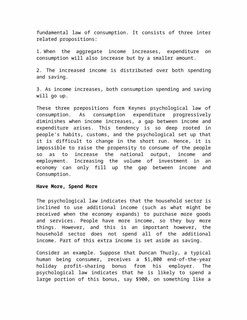
The Consumption Line

The psychological law is embodied in the consumption function (or consumption line), such as the one displayed in the exhibit to the right. The vertical axis measures consumption expenditures. The horizontal axis measures income generated from production.

The red line, labeled C, is the consumption line. This line has a positive slope, indicating that greater levels of consumption expenditures result from greater levels of income. Moreover, the slope of the line is numerically less than one. That is, the change in consumption expenditures is less than the change in income.

Figure 1

The relation between consumption and income is termed induced consumption and is measured by the marginal propensity to consume, which is the numerical measure of the slope of the consumption line.

Effective Demand

Consumption Line

This psychological law is most important for the Keynesian economic notion of effective demand. Effective demand indicates that aggregate expenditures, especially consumption expenditures, are based on the actual income generated by production and not on the income that would be generated if all resources were fully employed.

Effective demand was proposed first by Thomas Malthus and later by Keynes as a counter to Say's law that supply creates its own demand. Effective demand, in contrast, suggests that demand creates its own supply (at least up to full employment).

This might seem like a subtle, insignificant distinction, but it helps to separate classical economics and its assurance of full employment from Keynesian economics and the distinct possibility of persistent unemployment.

1.4 LAW OF CONSUMPTION IN SHORT AND LONG RUN

The Keynesian Theory of consumption is that current real disposable income is the most important determinant of consumption in the short run. Real Income is money income adjusted for inflation. It is a measure of the quantity of goods and services that consumers have buy with their income (or budget).

For example, a 10% rise in money income may be matched by a 10% rise in inflation. This means that real income (the quantity or volume of goods and services that can be bought) has remained constant.

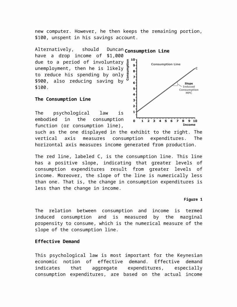
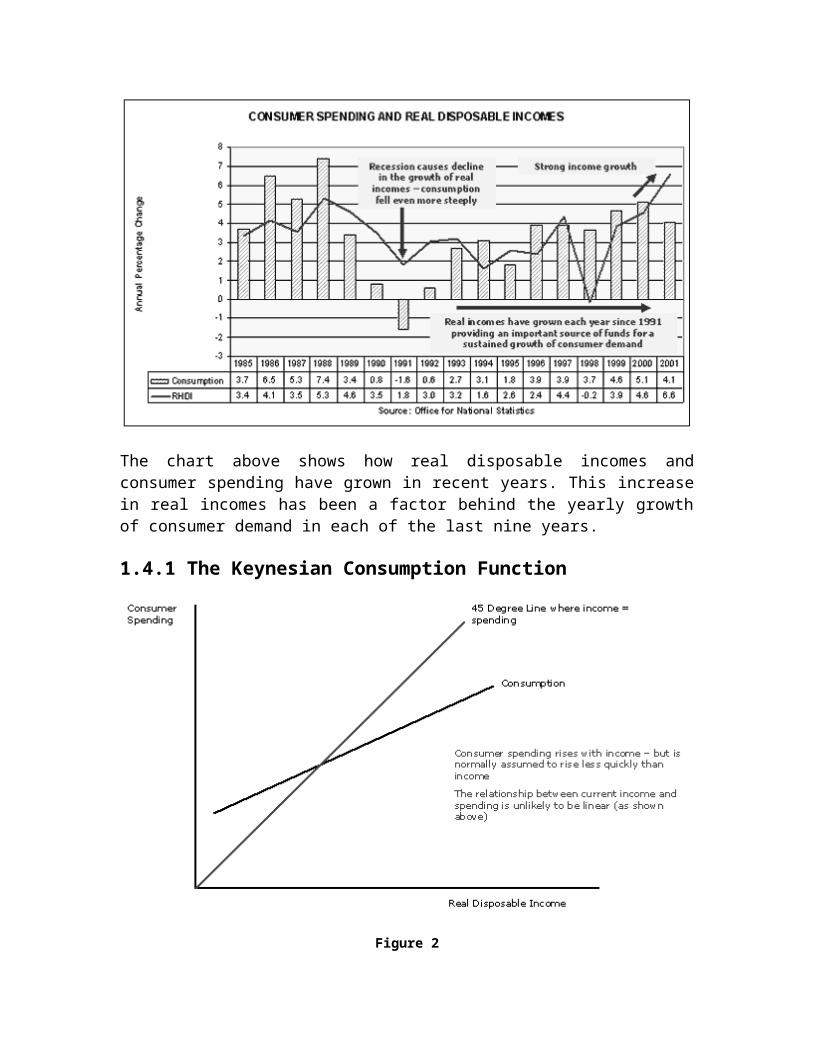
The chart above shows how real disposable incomes and consumer spending have grown in recent years. This increase in real incomes has been a factor behind the yearly growth of consumer demand in each of the last nine years.

1.4.1 The Keynesian Consumption Function

Figure 2

Disposable Income (Yd) = Gross Income - (Deductions from Direct Taxation + Benefits)

The standard Keynesian consumption function is as follows:

C = a + c Yd where,

C= Consumer expenditure

a = autonomous consumption. This is the level of consumption that would take place even if income was zero. If an individual's income fell to zero some of his existing spending could be sustained by using savings. This is known as dis-saving.

c = marginal propensity to consume (mpc). This is the change in consumption divided by the change in income. Simply, it is the percentage of each additional pound earned that will be spent.

There is a positive relationship between disposable income (Yd) and consumer spending (Ct). The gradient of the consumption curve gives the marginal propensity to consume. As income rises, so does total consumer demand.

A change in the marginal propensity to consume causes a pivotal change in the consumption function. In this case the marginal propensity to consume has fallen leading to a fall in consumption at each level of income. This is shown below:

1.4.2 Key Consumption Definitions

Average propensity to consume = Total consumption divided by total income

Average propensity to Save = Total savings divided by total income (also known as the Saving Ratio

A Shift in the Consumption Function

Figure 3

The consumption - income relationship changes when other factors than income change - for example a rise in interest rates or a fall in consumer confidence might lead to a fall in consumption spending at each level of income.

A rise in household wealth or a rise in consumer's expectations might lead to an increased level of consumer demand at each income level (an upward shift in the consumption curve).

Four Approaches to the Consumption Function

1)      Absolute Income Hypotheses

2)      Relative Income Hypothesis (James Duesenberry 1949 ~ From Thorstein Veblen)

3)      Permanent Income Hypothesis (Friedman)

4)      Life Cycle Hypothesis (Ando & Modigliani)

Theories 3 and 4 are most compatible with Neo-classical economics.

1.4.3 The Absolute Income Hypothesis

CD = a = bYt

 The current level of consumption is a straightforward function, driven by the current level of income. This implies that people adapt instantaneously to income changes.

- there is rapid adaptation to income changes

- the elasticity of consumption to current income changes

The elasticity with respect to current income in other theories will be less. They reduce the sensitivity to current income flows.

Figure 4

 1.4.4 The Relative Income Hypothesis

The Duesenberry approach says that people are not just concerned about absolute levels of possession. They are in fact concerned about their possessions relative to others, “Keeping up with the Jones.”

People are not necessarily happier if they have more money. They do however report higher happiness if they have more relative to others.

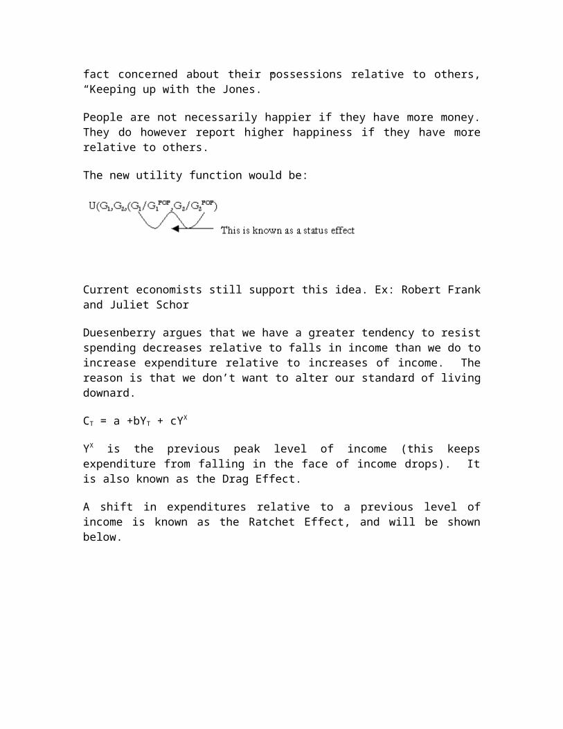
The new utility function would be:

Current economists still support this idea. Ex: Robert Frank and Juliet Schor

Duesenberry argues that we have a greater tendency to resist spending decreases relative to falls in income than we do to increase expenditure relative to increases of income. The reason is that we don’t want to alter our standard of living downard.

CT = a +bYT + cYX

YX is the previous peak level of income (this keeps expenditure from falling in the face of income drops). It is also known as the Drag Effect.

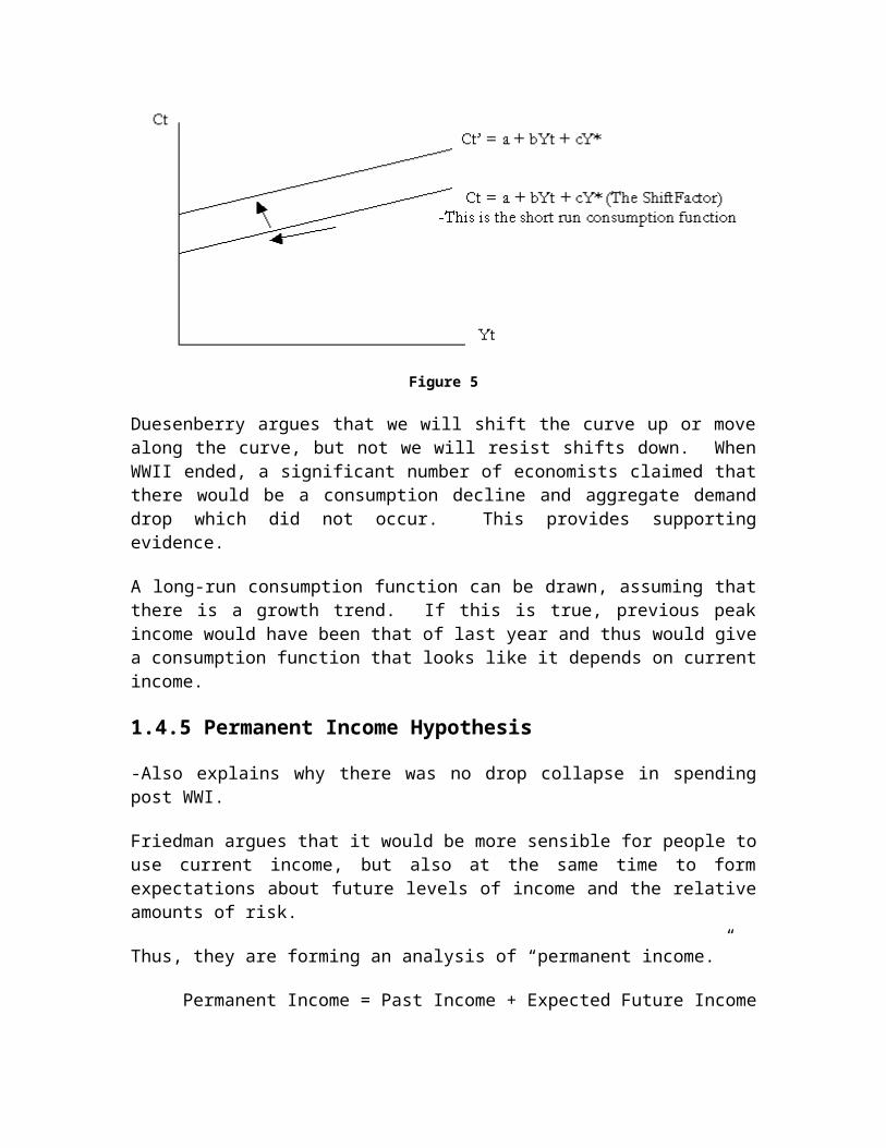
A shift in expenditures relative to a previous level of income is known as the Ratchet Effect, and will be shown below.

Figure 5

Duesenberry argues that we will shift the curve up or move along the curve, but not we will resist shifts down. When WWII ended, a significant number of economists claimed that there would be a consumption decline and aggregate demand drop which did not occur. This provides supporting evidence.

A long-run consumption function can be drawn, assuming that there is a growth trend. If this is true, previous peak income would have been that of last year and thus would give a consumption function that looks like it depends on current income.

1.4.5 Permanent Income Hypothesis

-Also explains why there was no drop collapse in spending post WWI.

Friedman argues that it would be more sensible for people to use current income, but also at the same time to form expectations about future levels of income and the relative amounts of risk.

Thus, they are forming an analysis of “permanent income.”

Permanent Income = Past Income + Expected Future Income

Transitory Income – Income that is earned in excess of, or perceived as an unexpected windfall is called as transitory income. If you get income not equal to what you expected or what you don’t expect to get again.

So, he argues that we tend to spend more out of permanent income than out of transitory.

In the Friedman analysis, he treats people as forming their level of expected future income based on their past incomes. This is known as adaptive expectations.

Adaptive Expectations – looking forward in time using past expectations. In this case, we use a distributed lag of past income.

YPt+1 ® E(Yt+1) = B0Yt + B1Yt-1 + B2Yt-2…

Where B0 > B1 > B2

It is also possible to add a constraint: B0 + B1 + B2 + B3 + … Bn = 1

This is expected income, the actual income can be thought of as:

Yt-1 – Ypt+1 = Yt

t+1

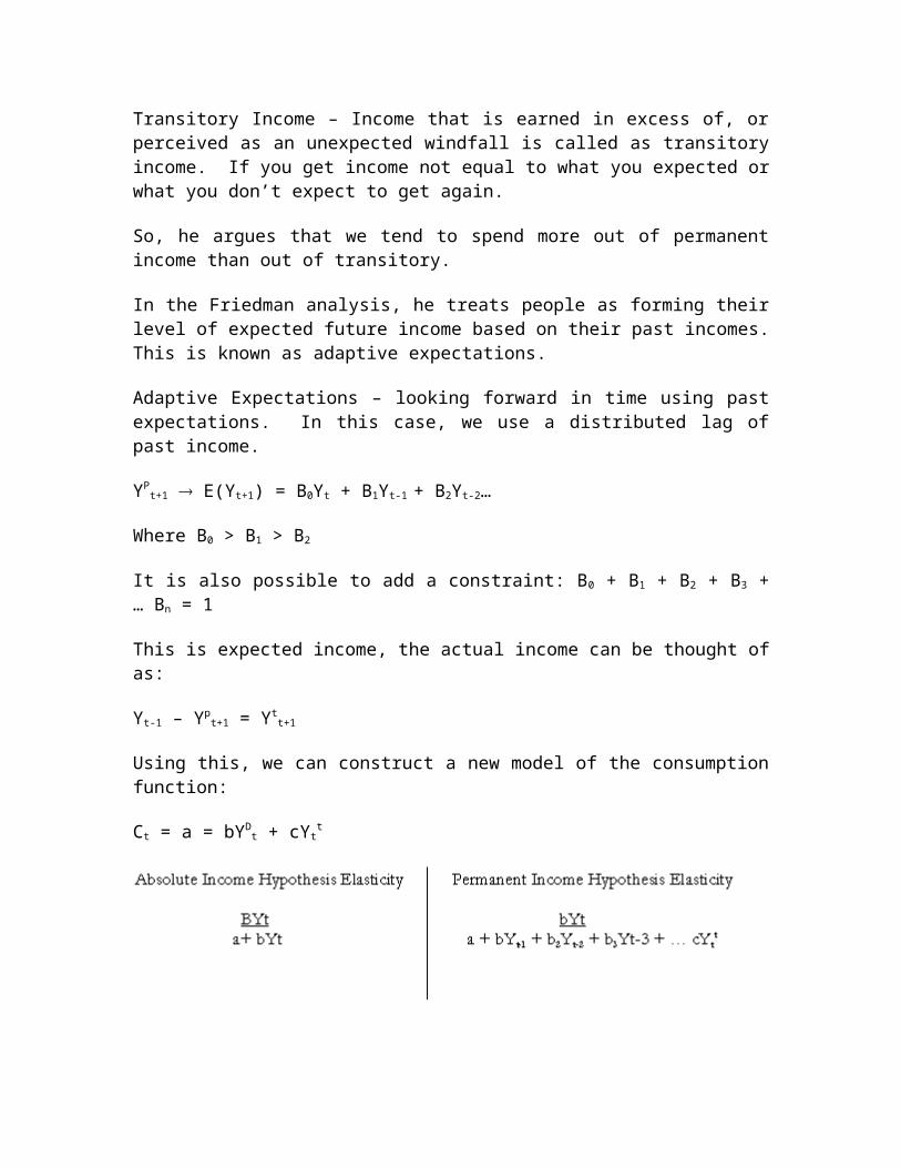
Using this, we can construct a new model of the consumption function:  

Ct = a = bYDt + cYt

t

There are other factors that people can look at to think about future levels of income. For example, people can think about future interest rates and their effect on their income stream. If you were Friedman, you would do this by using a distributed lag of past incomes.

1.4.6 The Life Cycle Hypothesis

This is primarily attributed to Ando and Modigliani

The basic notion is that consumption spending will be smooth in the face of an erratic stream of income.

Figure 6

Working Phase:

1. Maintain current consumption, pay off debt from youth years 2. Maintain current consumption, build up reserves

Age distribution now matters when we look at consumption, and in general, the propensity to consume. Debt and wealth are also taken into account when we look at the

propensity to consume. The dependence structure of the population will affect or influence consumption patterns.

Lester Thurow (1976) – argued that this model doesn’t work because it doesn’t presume there is any motive for building wealth other than consumption. Thurow argues that their real motivation is status and power (both internal and external to the family).

The permanent income hypothesis bears a resemblance to the life-cycle hypothesis in that in some sense, in both hypotheses, the individuals must behave as if they have some sense of the future.

To sum it all we can say that, an economic model of the proportion of income spent on consumption. John Maynard Keynes pioneered in this area with the absolute income hypothesis, which states that consumption is solely a function of current disposable income. Divergence between Keynes's predictions and subsequent empirical data, especially over the long run, has led to a number of other theories of consumption—most prominently, those based relative income (Duesenberry), permanent income ( Milton Friedman ), and life-cycle income (Modigliani and Brumberg).

Keynes argued that any change in income results in a smaller change in consumption—i.e., the marginal propensity to consume is less than one. He also argued that the marginal propensity to consume is less than the average propensity to consume, which implies that consumption declines as a percentage of income as income rises. Short-run studies broadly support a consumption function of this form, but long-run data suggest that the average and the marginal propensities to consume are roughly the same.

The relative income hypothesis conceives consumption in relation to the income of other households and past income. The first implies that the proportion of income consumed remains constant provided that a household's position on the income distribution curve holds constant in the long run. This is consistent with long-run evidence. Higher up the income curve, however, there is a lower average propensity to consume. The second part of the hypothesis suggests that households find it easier to adjust to rising incomes than falling incomes. There is, in other words, a “ratchet effect” that holds up consumption when income declines.

The measurement of permanent and lifetime income has become a central issue in recent attempts to specify the consumption function. The permanent income hypothesis postulates that consumption depends on the total income and wealth that an individual expects to earn over his or her lifetime. The life-cycle hypothesis assumes that individuals consume a constant proportion of the present value of lifetime income as measured in a number of financially distinct periods of life, such as youth, middle age, and old age. Empirical research in this area has proved challenging, because theories of consumption generally include the long-term “use” of durable goods. Consumption data, however, focus primarily on current purchases, or consumption expenditure.

Activity 1

1. What do you understand by law of consumption? Discuss in view of Keynes.2. Discuss the contribution of Keynes in economics and quote his different

approaches to consumption function.

3. Distinguish between relative income hypothesis and permanent hypothesis.

4. Write a short note on life cycle hypothesis.

1.5 SUMMARY

The unit started with introducing the Keynesian economics which is perceived as a macroeconomic theory based on the ideas of 20th-century British economist John Maynard Keynes. Keynesian economics argues that private sector decisions sometimes lead to inefficient macroeconomic outcomes. Followed by this the consumption function is explained as a single mathematical function used to express consumer spending. Psychological law of consumption function is described along with possible implications in the later section. Law of consumption in short and long run has been discussed with its four approaches called absolute Income Hypotheses, Relative Income Hypothesis, Permanent Income Hypothesis and life Cycle Hypothesis.

1.6 FURTHER READINGS

J.M. Keynes (1937) "The General Theory of Employment", Quarterly Journal of Economics, Vol. 51

Mary S. Morgan, The History of Econometric Ideas, Cambridge University Press, 1991

Paul Mattick, Marx and Keynes: The Limits of Mixed Economy, Boston, Porter Sargent, 1969

UNIT 2

INVESTMENT FUNCTION AND KEYNES THEORY OF EMPLOYMENT

Objectives

After studying this unit you should be able to:

Understand the approach and scope investment in Keynes theory of employment Know the relevance of excessive savings in the theory and in practice

Appreciate the approaches to marginal efficiency and rate of return.

Be aware about the concept of multiplier accelerator

Explain the role of inflation in investment decisions

Describe the policy measures and their relevance in investment decisions

Structure

2.1 Introduction2.2 Excessive savings2.3 Rate of return and marginal efficiency2.4 The multiplier accelerator and investment behavior2.5 Inflation and investment decisions2.6 Policy measures and investment2.7 Summary2.8 Further readings

2.1 INTRODUCTION TO KEYNESIAN THEORY OF INVESTMENT

The Keynesian theory of investment places emphasis on the importance of interest rates in investment decisions. But other factors also enter into the model - not least the expected profitability of an investment project.

Changes in interest rates should have an effect on the level of planned investment undertaken by private sector businesses in the economy.

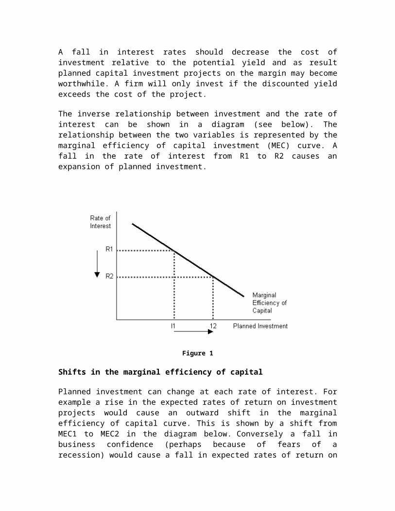
A fall in interest rates should decrease the cost of investment relative to the potential yield and as result planned capital investment projects on the margin may become worthwhile. A firm will only invest if the discounted yield exceeds the cost of the project.

The inverse relationship between investment and the rate of interest can be shown in a diagram (see below). The relationship between the two variables is represented by the marginal efficiency of capital investment (MEC) curve. A fall in the rate of interest from R1 to R2 causes an expansion of planned investment.

 

Figure 1

Shifts in the marginal efficiency of capital

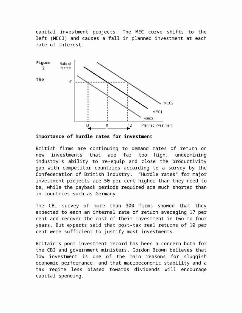
Planned investment can change at each rate of interest. For example a rise in the expected rates of return on investment projects would cause an outward shift in the marginal efficiency of capital curve. This is shown by a shift from MEC1 to MEC2 in the diagram below. Conversely a fall in business confidence (perhaps because of fears of a recession) would cause a fall in expected rates of return on capital investment projects. The MEC curve shifts to the left (MEC3) and causes a fall in planned investment at each rate of interest.

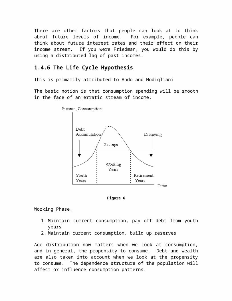
Figure 2

The importance of hurdle rates for investment

British firms are continuing to demand rates of return on new investments that are far too high, undermining industry's ability to re-equip and close the productivity gap with competitor countries according to a survey by the Confederation of British Industry. "Hurdle rates" for major investment projects are 50 per cent higher than they need to be, while the payback periods required are much shorter than in countries such as Germany.

The CBI survey of more than 300 firms showed that they expected to earn an internal rate of return averaging 17 per cent and recover the cost of their investment in two to four years. But experts said that post-tax real returns of 10 per cent were sufficient to justify most investments.

Britain's poor investment record has been a concern both for the CBI and government ministers. Gordon Brown believes that low investment is one of the main reasons for sluggish economic performance, and that macroeconomic stability and a tax regime less biased towards dividends will encourage capital spending.  

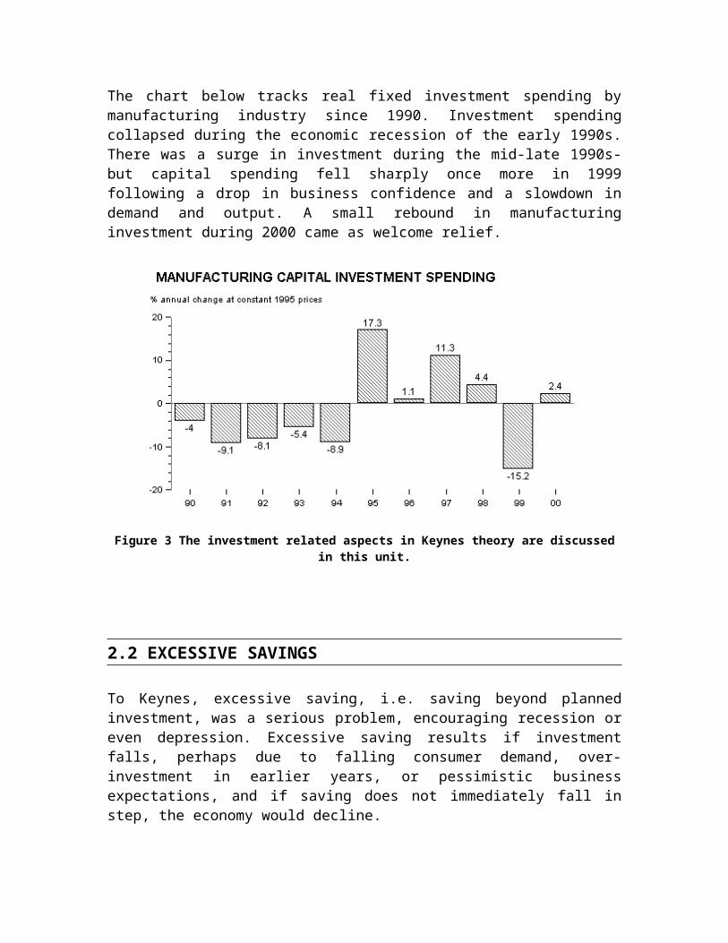
The chart below tracks real fixed investment spending by manufacturing industry since 1990. Investment spending collapsed during the economic recession of the early 1990s. There was a surge in investment during the mid-late 1990s- but capital spending fell sharply once more in 1999 following a drop in business confidence and a slowdown in demand and output. A small rebound in manufacturing investment during 2000 came as welcome relief.

Figure 3 The investment related aspects in Keynes theory are discussed in this unit.

2.2 EXCESSIVE SAVINGS

To Keynes, excessive saving, i.e. saving beyond planned investment, was a serious problem, encouraging recession or even depression. Excessive saving results if investment falls, perhaps due to falling consumer demand, over-investment in earlier years, or pessimistic business expectations, and if saving does not immediately fall in step, the economy would decline.

Figure 4

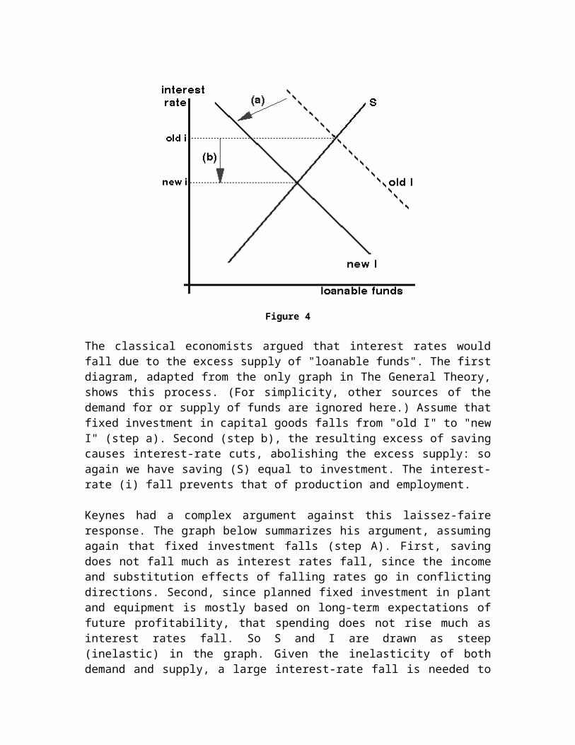
The classical economists argued that interest rates would fall due to the excess supply of "loanable funds". The first diagram, adapted from the only graph in The General Theory, shows this process. (For simplicity, other sources of the demand for or supply of funds are ignored here.) Assume that fixed investment in capital goods falls from "old I" to "new I" (step a). Second (step b), the resulting excess of saving causes interest-rate cuts, abolishing the excess supply: so again we have saving (S) equal to investment. The interest-rate (i) fall prevents that of production and employment.

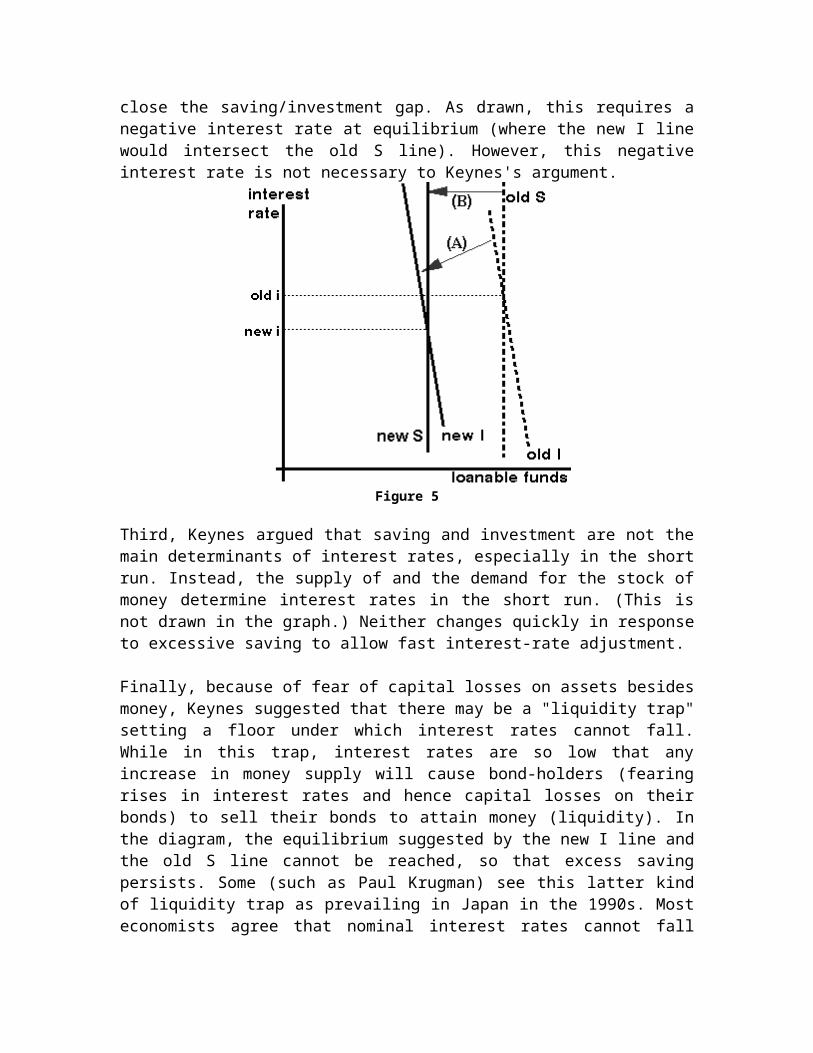
Keynes had a complex argument against this laissez-faire response. The graph below summarizes his argument, assuming again that fixed investment falls (step A). First, saving does not fall much as interest rates fall, since the income and substitution effects of falling rates go in conflicting directions. Second, since planned fixed investment in plant and equipment is mostly based on long-term expectations of future profitability, that spending does not rise much as interest rates fall. So S and I are drawn as steep (inelastic) in the graph. Given the inelasticity of both demand and supply, a large interest-rate fall is needed to close the saving/investment gap. As drawn, this requires a negative interest rate at equilibrium (where the new I line would intersect the old S line). However, this negative interest rate is not necessary to Keynes's argument.

Figure 5

Third, Keynes argued that saving and investment are not the main determinants of interest rates, especially in the short run. Instead, the supply of and the demand for the stock of money determine interest rates in the short run. (This is not drawn in the graph.) Neither changes quickly in response to excessive saving to allow fast interest-rate adjustment.

Finally, because of fear of capital losses on assets besides money, Keynes suggested that there may be a "liquidity trap" setting a floor under which interest rates cannot fall. While in this trap, interest rates are so low that any increase in money supply will cause bond-holders (fearing rises in interest rates and hence capital losses on their bonds) to sell their bonds to attain money (liquidity). In the diagram, the equilibrium suggested by the new I line and the old S line cannot be reached, so that excess saving persists. Some (such as Paul Krugman) see this latter kind of liquidity trap as prevailing in Japan in the 1990s. Most economists agree that nominal interest rates cannot fall below zero, however, some economists (particularly those from the Chicago school) reject the existence of a liquidity trap.

Even if the liquidity trap does not exist, there is a fourth (perhaps most important) element to Keynes's critique. Saving involves not spending all of one's income. It thus means insufficient demand for business output, unless it is balanced by other sources of demand, such as fixed investment. Thus, excessive saving corresponds to an unwanted accumulation of inventories, or what classical economists called a general glut. This pile-up of unsold goods and materials encourages businesses to decrease both production and employment. This in turn lowers people's incomes—and saving, causing a leftward shift in the S line in the diagram (step B). For Keynes, the fall in income did most of the job by ending excessive saving and allowing the loanable funds market to attain equilibrium. Instead of interest-rate adjustment solving the problem, a recession does so. Thus in the diagram, the interest-rate change is small.

Whereas the classical economists assumed that the level of output and income was constant and given at any one time (except for short-lived deviations), Keynes saw this as the key variable that adjusted to equate saving and investment.Finally, a recession undermines the business incentive to engage in fixed investment. With falling incomes and demand for products, the desired demand for factories and equipment (not to mention housing) will fall. This accelerator effect would shift the 1ST

line to the left again, a change not shown in the diagram above. This recreates the problem of excessive saving and encourages the recession to continue.In sum, to Keynes there is interaction between excess supplies in different markets, as unemployment in labor markets encourages excessive saving—and vice-versa. Rather than prices adjusting to attain equilibrium, the main story is one of quantity adjustment allowing recessions and possible attainment of underemployment equilibrium.

2.3 RATE OF RETURN AND MARGINAL EFFICIENCY

In his General Theory, John Maynard Keynes (1936: Ch.11) proposed an investment function of the sort I = I0 + I(r) where the relationship between investment and interest rate was of a rather naive form. Firms were presumed to "rank" various investment projects depending on their "internal rate of return" (or "marginal efficiency of investment") and thereafter, faced with a given rate of interest, chose those projects whose internal rate of return exceeded the rate of interest. With an infinite number of projects available, this amounted to arguing that firms would invest until their marginal efficiency of investment was equal to the rate of interest, i.e. MEI = r.

More elaborate considerations of Keynes's theory, however, were forced to ask what is the internal rate of return? This is far from evident. Keynes defined the internal rate of return as the "marginal efficiency of capital", which Abba Lerner (1944, 1953), more accurately, rebaptized as the "marginal efficiency of investment" (MEI). Keynes claimed that this could be defined as follows:

"I define the marginal efficiency of capital as being equal to the rate of discount which would make the present value of the series of annuities given by the returns expected from the capital asset during its life just equal its supply price" (Keynes , 1936: p. 135)

In constrast, Keynes defines the "supply price of the capital asset...not the market price at which an asset of the type in question can actually be purchased in the market, but the price which would just induce a manufacturer newly to produce an additional unit of such assets, i.e. what is sometimes called its replacement cost" (1936: p.135). Consequently:

"The relation between the prospective yield of a capital asset and its supply price or replacement cost, i.e. the relation between the prospective yield of one more unit of that type of capital and the cost of producing that unit, furnishes us with the marginal efficiency of capital of that type" (Keynes , 1936: p.135).

When a man buys an investment or capital-asset, he purchases the right to the series of prospective returns, which he expects to obtain from selling its output, after deducting the running expenses of obtaining that output, during the life of the asset. This series of annuities Q 1 ,  Q 2 , . . .  Q n it is convenient to call the prospective yield of the investment.

Over against the prospective yield of the investment we have the supply price of the capital-asset, meaning by this, not the market-price at which an asset of the type in question can actually be purchased in the market, but the price which would just induce a manufacturer newly to produce an additional unit of such assets, i.e. what is sometimes called its replacement cost . The relation between the prospective yield of a capital-asset and its supply price or replacement cost, i.e. the relation between the prospective yield of one more unit of that type of capital and the cost of producing that unit, furnishes us with the marginal efficiency of capital of that type. More precisely, I define the marginal efficiency of capital as being equal to that rate of discount which would make the present value of the series of annuities given by the returns expected from the capital-asset during its life just equal to its supply price. This gives us the marginal efficiencies of particular types of capital-assets. The greatest of these marginal efficiencies can then be regarded as the marginal efficiency of capital in general.

The reader should note that the marginal efficiency of capital is here defined in terms of the expectation of yield and of the current supply price of the capital-asset. It depends on the rate of return expected to be obtainable on money if it were invested in a newly produced asset; not on the historical result of what an investment has yielded on its original cost if we look back on its record after its life is over.

If there is an increased investment in any given type of capital during any period of time, the marginal efficiency of that type of capital will diminish as the investment in it is increased, partly because the prospective yield will fall as the supply of that type of capital is increased, and partly because, as a rule, pressure on the facilities for producing that type of capital will cause its supply price to increase; the second of these factors being usually the more important in producing equilibrium in the short run, but the longer the period in view the more does the first factor take its place. Thus for each type of capital we can build up a schedule, showing by how much investment in it will have to increase within the period, in order that its marginal efficiency should fall to any given figure. We can then aggregate these schedules for all the different types of capital, so as to provide a schedule relating the rate of aggregate investment to the corresponding marginal efficiency of capital in general which that rate of investment will establish. We shall call this the investment demand-schedule; or, alternatively, the schedule of the marginal efficiency of capital.

Now it is obvious that the actual rate of current investment will be pushed to the point where there is no longer any class of capital-asset of which the marginal efficiency exceeds the current rate of interest. In other words, the rate of investment will be pushed to the point on the investment demand-schedule where the marginal efficiency of capital in general is equal to the market rate of interest. 

The same thing can also be expressed as follows. If Qr is the prospective yield from an asset at time r , and d r is the present value of 1 deferred r years at the current rate of interest, Qr dr is the demand price of the investment; and investment will be carried to the point where Qr dr becomes equal to the supply price of the investment as defined above. If, on the other hand, Qr dr falls short of the supply price, there will be no current investment in the asset in question.

It follows that the inducement to invest depends partly on the investment demand-schedule and partly on the rate of interest.

How is the above definition of the marginal efficiency of capital related to common usage? The Marginal Productivity or Yield or Efficiency or Utility of Capital is familiar terms which we have all frequently used. But it is not easy by searching the literature of economics to find a clear statement of what economists have usually intended by these terms.

There are at least three ambiguities to clear up. There is, to begin with, the ambiguity whether we are concerned with the increment of physical product per unit of time due to the employment of one more physical unit of capital, or with the increment of value due to the employment of one more value unit of capital. The former involves difficulties as to the definition of the physical unit of capital, which I believe to be both insoluble and unnecessary. It is, of course, possible to say that ten labourers will raise more wheat from a given area when they are in a position to make use of certain additional machines; but I know no means of reducing this to an intelligible arithmetical ratio which does not bring in values. Nevertheless many discussions of this subject seem to be mainly concerned with the physical productivity of capital in some sense, though the writers fail to make them clear.

Secondly, there is the question whether the marginal efficiency of capital is some absolute quantity or a ratio. The contexts in which it is used and the practice of treating it as being of the same dimension as the rate of interest seem to require that it should be a ratio. Yet it is not usually made clear what the two terms of the ratio are supposed to be.

Finally, there is the distinction, the neglect of which has been the main cause of confusion and misunderstanding, between the increment of value obtainable by using an additional quantity of capital in the existing situation, and the series of increments which it is expected to obtain over the whole life of the additional capital asset; i.e. the distinction between Q1 and the complete series Q1 ,  Q2 , . . .  Qr , . . . .This involves the whole question of the place of expectation in economic theory. Most discussions of the marginal efficiency of capital seem to pay no attention to any member of the series except Q1 . Yet this cannot be legitimate except in a static theory, for which all the Q's are equal. The ordinary theory of distribution, where it is assumed that capital is getting now its marginal productivity (in some sense or other), is only valid in a stationary state. The aggregate current return to capital has no direct relationship to its marginal efficiency; whilst its current return at the margin of production (i.e. the return to capital which enters

into the supply price of output) is its marginal user cost, which also has no close connection with its marginal efficiency.

There is, as I have said above, a remarkable lack of any clear account of the matter. At the same time I believe that the definition which I have given above is fairly close to what Marshall intended to mean by the term. The phrase which Marshall himself uses is "marginal net efficiency" of a factor of production; or, alternatively, the "marginal utility of capital". The following is a summary of the most relevant passage which I can find in his Principles (6th ed. pp. 519 520). I have run together some non-consecutive sentences to convey the gist of what he says:

"In a certain factory extra 100 worth of machinery can be applied so as not to involve any other extra expense, and so as to add annually 3 worth to the net output of the factory after allowing for its own wear and tear. If the investors of capital push it into every occupation in which it seems likely to gain a high reward; and if, after this has been done and equilibrium has been found, it still pays and only just pays to employ this machinery, we can infer from this fact that the yearly rate of interest is 3 per cent. But illustrations of this kind merely indicate part of the action of the great causes which govern value. They cannot be made into a theory of interest, any more than into a theory of wages, without reasoning in a circle. . . Suppose that the rate of interest is 3 per cent. per annum on perfectly good security; and that the hat-making trade absorbs a capital of one million pounds. This implies that the hat-making trade can turn the whole million pounds' worth of capital to so good account that they would pay 3 per cent. per annum net for the use of it rather than go without any of it. There may be machinery which the trade would have refused to dispense with if the rate of interest had been 20 per cent. per annum. If the rate had been 10 per cent., more would have been used; if it had been 6 per cent., still more; if 4 per cent. still more; and finally, the rate being 3 per cent., they use more still. When they have this amount, the marginal utility of the machinery, i.e. the utility of that machinery which it is only just worth their while to employ, is measured by 3 per cent."

It is evident from the above that Marshall was well aware that we are involved in a circular argument if we try to determine along these lines what the rate of interest actually is. In this passage he appears to accept the view set forth above, that the rate of interest determines the point to which new investment will be pushed, given the schedule of the marginal efficiency of capital. If the rate of interest is 3 per cent, this means that no one will pay 100 for a machine unless he hopes thereby to add 3 to his annual net output after allowing for costs and depreciation.

Although he does not call it the "marginal efficiency of capital", Professor Irving Fisher has given in his Theory of Interest (1930) a definition of what he calls "the rate of return over cost" which is identical with my definition. "The rate of return over cost", he writes,  "is that rate which, employed in computing the present worth of all the costs and the present worth of all the returns, will make these two equal." Professor Fisher explains that the extent of investment in any direction will depend on a comparison between the rate of return over cost and the rate of interest. To induce new investment "the rate of return over cost must exceed the rate of interest". "This new magnitude (or factor) in our

study plays the central role on the investment opportunity side of interest theory." Thus Professor Fisher uses his "rate of return over cost" in the same sense and for precisely the same purpose as I employ "the marginal efficiency of capital".

The most important confusion concerning the meaning and significance of the marginal efficiency of capital has ensued on the failure to see that it depends on the prospective yield of capital, and not merely on its current yield. This can be best illustrated by pointing out the effect on the marginal efficiency of capital of an expectation of changes in the prospective cost of production, whether these changes are expected to come from changes in labour cost, i.e. in the wage-unit, or from inventions and new technique. The output from equipment produced to-day will have to compete, in the course of its life, with the output from equipment produced subsequently, perhaps at a lower labour cost, perhaps by an improved technique, which is content with a lower price for its output and will be increased in quantity until the price of its output has fallen to the lower figure with which it is content. Moreover, the entrepreneur's profit (in terms of money) from equipment, old or new, will be reduced, if all output comes to be produced more cheaply. In so far as such developments are foreseen as probable, or even as possible, the marginal efficiency of capital produced to-day is appropriately diminished.

This is the factor through which the expectation of changes in the value of money influences the volume of current output. The expectation of a fall in the value of money stimulates investment, and hence employment generally, because it raises the schedule of the marginal efficiency of capital, i.e. the investment demand-schedule; and the expectation of a rise in the value of money is depressing, because it lowers the schedule of the marginal efficiency of capital.

This is the truth which lies behind Professor Irving Fisher's theory of what he originally called "Appreciation and Interest" the distinction between the money rate of interest and the real rate of interest where the latter is equal to the former after correction for changes in the value of money. It is difficult to make sense of this theory as stated, because it is not clear whether the change in the value of money is or is not assumed to be foreseen. There is no escape from the dilemma that, if it is not foreseen, there will be no effect on current affairs; whilst, if it is foreseen, the prices of existing goods will be forthwith so adjusted that the advantages of holding money and of holding goods are again equalised, and it will be too late for holders of money to gain or to suffer a change in the rate of interest which will offset the prospective change during the period of the loan in the value of the money lent. For the dilemma is not successfully escaped by Professor Pigou's expedient of supposing that the prospective change in the value of money is foreseen by one set of people but not foreseen by another.

The mistake lies in supposing that it is the rate of interest on which prospective changes in the value of money will directly react, instead of the marginal efficiency of a given stock of capital. The prices of existing assets will always adjust themselves to changes in expectation concerning the prospective value of money. The significance of such changes in expectation lies in their effect on the readiness to produce new assets through their reaction on the marginal efficiency of capital. The stimulating effect of the expectation of

higher prices is due, not to its raising the rate of interest (that would be a paradoxical way of stimulating output in so far as the rate of interest rises, the stimulating effect is to that extent offset), but to its raising the marginal efficiency of a given stock of capital. If the rate of interest were to rise pari passu with the marginal efficiency of capital, there would be no stimulating effect from the expectation of rising prices. For the stimulus to output depends on the marginal efficiency of a given stock of capital rising relatively to the rate of interest. Indeed Professor Fisher's theory could be best re-written in terms of a "real rate of interest" defined as being the rate of interest which would have to rule, consequently on a change in the state of expectation as to the future value of money, in order that this change should have no effect on current output.

It is worth noting that an expectation of a future fall in the rate of interest will have the effect of lowering the schedule of the marginal efficiency of capital; since it means that the output from equipment produced to-day will have to compete during part of its life with the output from equipment which is content with a lower return. This expectation will have no great depressing effect, since the expectations, which are held concerning the complex of rates of interest for various terms which will rule in the future, will be partially reflected in the complex of rates of interest which rule to-day. Nevertheless there may be some depressing effect, since the output from equipment produced to-day, which will emerge towards the end of the life of this equipment, may have to compete with the output of much younger equipment which is content with a lower return because of the lower rate of interest which rules for periods subsequent to the end of the life of equipment produced to-day.

It is important to understand the dependence of the marginal efficiency of a given stock of capital on changes in expectation, because it is chiefly this dependence which renders the marginal efficiency of capital subject to the somewhat violent fluctuations which are the explanation of the Trade Cycle.

Two types of risk affect the volume of investment which has not commonly been distinguished, but which it is important to distinguish. The first is the entrepreneur's or borrower's risk and arises out of doubts in his own mind as to the probability of his actually earning the prospective yield for which he hopes. If a man is venturing his own money, this is the only risk which is relevant.

But where a system of borrowing and lending exists, by which I mean the granting of loans with a margin of real or personal security, a second type of risk is relevant which we may call the lender's risk. This may be due either to moral hazard, i.e. voluntary default or other means of escape, possibly lawful, from the fulfilment of the obligation, or to the possible insufficiency of the margin of security, i.e. involuntary default due to the disappointment of expectation. A third source of risk might be added, namely, a possible adverse change in the value of the monetary standard which renders a money-loan to this extent less secure than a real asset; though all or most of this should be already reflected, and therefore absorbed, in the price of durable real assets.

Now the first type of risk is, in a sense, a real social cost, though susceptible to diminution by averaging as well as by an increased accuracy of foresight. The second, however, is a pure addition to the cost of investment which would not exist if the borrower and lender was the same person. Moreover, it involves in part a duplication of a proportion of the entrepreneur's risk, which is added twice to the pure rate of interest to give the minimum prospective yield which will induce the investment. For if a venture is a risky one, the borrower will require a wider margin between his expectation of yield and the rate of interest at which he will think it worth his while to borrow; whilst the very same reason will lead the lender to require a wider margin between what he charges and the pure rate of interest in order to induce him to lend (except where the borrower is so strong and wealthy that he is in a position to offer an exceptional margin of security). The hope of a very favourable outcome, which may balance the risk in the mind of the borrower, is not available to solace the lender.

This duplication of allowance for a portion of the risk has not hitherto been emphasised, so far as I am aware; but it may be important in certain circumstances. During a boom the popular estimation of the magnitude of both these risks, both borrower's risk and lender's risk, is apt to become unusually and imprudently low.

The schedule of the marginal efficiency of capital is of fundamental importance because it is mainly through this factor (much more than through the rate of interest) that the expectation of the future influences the present. The mistake of regarding the marginal efficiency of capital primarily in terms of the current yield of capital equipment, which would be correct only in the static state where there is no changing future to influence the present, has had the result of breaking the theoretical link between to-day and to-morrow. Even the rate of interest is, virtually,  a current phenomenon; and if we reduce the marginal efficiency of capital to the same status, we cut ourselves off from taking any direct account of the influence of the future in our analysis of the existing equilibrium.

The fact that the assumptions of the static state often underlie present-day economic theory, imports into it a large element of unreality. But the introduction of the concepts of user cost and of the marginal efficiency of capital, as defined above, will have the effect, I think, of bringing it back to reality, whilst reducing to a minimum the necessary degree of adaptation.

It is by reason of the existence of durable equipment that the economic future is linked to the present. It is, therefore, consonant with, and agreeable to, our broad principles of thought, that the expectation of the future should affect the present through the demand price for durable equipment.

2.4 THE MULTIPLIER ACCELERATOR AND INVESTMENT BEHAVIOUR

An initial change in aggregate demand can have a much greater final impact on the level of equilibrium national income. This is commonly known as the multiplier effect and it comes about because injections of demand into the circular flow of income stimulate

further rounds of spending – in other words “one person’s spending is another’s income” – and this can lead to a much bigger effect on equilibrium output and employment.

Consider a £300 million increase in business capital investment – for example created when an overseas company decides to build a new production plant in the UK. This will set off a chain reaction of increases in expenditures. Firms who produce the capital goods that are purchased will experience an increase in their incomes and profits. If they in turn, collectively spend about 3/5 of that additional income, then £180m will be added to the incomes of others.

At this point, total income has grown by (£300m + (0.6 x £300m).

The sum will continue to increase as the producers of the additional goods and services realize an increase in their incomes, of which they in turn spend 60% on even more goods and services.

The increase in total income will then be (£300m + (0.6 x £300m) + (0.6 x £180m).

The process can continue indefinitely. But each time, the additional rise in spending and income is a fraction of the previous addition to the circular flow.

Multiplier effects can be seen when new investment and jobs are attracted into a particular town, city or region. The final increase in output and employment can be far greater than the initial injection of demand because of the inter-relationships within the circular flow.

2.4.1 The Multiplier and Keynesian Economics

The concept of the multiplier process became important in the 1930s when John Maynard Keynes suggested it as a tool to help governments to achieve full employment. This macroeconomic “demand-management approach”, designed to help overcome a shortage of business capital investment, measured the amount of government spending needed to reach a level of national income that would prevent unemployment.

The higher is the propensity to consume domestically produced goods and services, the greater is the multiplier effect. The government can influence the size of the multiplier through changes in direct taxes. For example, a cut in the basic rate of income tax will increase the amount of extra income that can be spent on further goods and services.

Another factor affecting the size of the multiplier effect is the propensity to purchase imports. If, out of extra income, people spend money on imports, this demand is not passed on in the form of extra spending on domestically produced output. It leaks away from the circular flow of income and spending.

The multiplier process also requires that there is sufficient spare capacity in the economy for extra output to be produced. If short-run aggregate supply is inelastic, the full

multiplier effect is unlikely to occur, because increases in AD will lead to higher prices rather than a full increase in real national output. In contrast, when SRAS is perfectly elastic a rise in aggregate demand causes a large increase in national output.

Figure 6

The construction boom and multiplier effects

A study has found that the British construction sector alone has driven a fifth of UK GDP growth in the past year and 34% of net job creation in the past two years. The construction boom has been caused by the combination of large projects like Terminal 5, the Channel Tunnel Rail Link, Wembley Stadium and the Scottish Parliament with a revival in house building, heavy expenditure by the public sector on new schools and hospitals and a surge in home improvement expenditure.

The study provides compelling evidence on the multiplier effects of major capital investment projects. 'One characteristic of construction activity is that it feeds through to

many other related businesses. It has "backward linkages" into the likes of building materials; steel, architectural services, legal services and insurance, and most of these linkages tend to result in jobs close to home. This makes a boom in construction peculiarly powerful in fuelling expansion in the economy - for a given lift in building orders, the multiplier effect may be well over two. This means that every building job created will generate at least two others in related areas and in downstream activities such as retailing, which benefits when building workers spend their wages. Other industries, particularly those where much of the output value comes in the form of imported components, might have a multiplier of less than 1.5 for new projects'.

The accelerator effect

Figure 7

Planned capital investment by private sector businesses is linked to the growth of demand for goods and services. When consumer or export demand is rising strongly, businesses

may increase investment to expand their production capacity and meet the extra demand. This process is known as the accelerator effect. But the accelerator effect can work in the other direction! A slowdown in consumer demand can create excess capacity and may lead to a fall in planned investment demand. A good example of this in recent years is the telecommunications industry. Capital investment in this sector surged to record highs in the second half of the 1990s, driven by a fast pace of technological advance and huge increases in the ICT budgets of corporations, small-to-medium sized businesses, and extra capital investment by the public sector (including education and health).

The telecommunications industry invested giant sums in building bigger and faster networks, but demand has slowed in the first three of the decade, leaving the industry with a vast amount of spare capacity (an under-utilisation of resources). Capital investment spending in the telecommunications industry has fallen sharply in the last three years – the accelerator mechanism working in reverse.

2.4.2 The Simple Multiplier Model

Suppose a factory with a payroll of $500,000 locates in a Lemmingville, a typical suburban community. Suppose further that the $500,000 is the only money that the factory spends in the community, that all employees live in Lemmingville, and that each person who lives there spends exactly one half of his income locally. By how much will the income of Lemmingville rise as a result of the new factory?

The $500,000 will be an addition to Lemmingville income. But the story does not end here because, by assumption, the people who earn the payroll will spend one half of the payroll, or $250,000, in the community. This $250,000 will become income for the shopkeepers, plumbers, lawyers, teachers, etc. Thus Lemmingville income will rise by at least $750,000. But the story does not end here either. The shopkeepers, plumbers, etc. who received the $250,000 will in turn spend one half of their new income locally, and this $125,000 will become income for other people in the community. Total Lemmingville income is now $875,000. The process will continue on and on, and as it does, total income will approach $1,000,000.

Notice that the initial half million in income expands to one million once in the system. There is a multiplier effect that is similar to the multiplier effect in the model of contingent behavior. The size of the multiplier in our suburb depends on the percentage of income people spend within the community. The smaller the percentage, the more quickly the extra income leaks out of the economy and the smaller the multiplier.

The Keynesian multiplier model applies to the national economy the logic by which a new factory can increase a town's income by a multiple of its payroll. Central in this model is an assumption about how people spend, the consumption function. The consumption function says that the amount people spend depends on their income, and that as income increases, so does consumption.

The table below illustrates a consumption function. It says that if people expect incomes of $10,000, they will spend $12,500. This amount of spending is possible if people plan to borrow or to dissave. (To dissave means to sell assets.) The table says that when expected income is $30,000, people will spend $27,500, which means that they plan to save $2,500.

Table 1: A Consumption FunctionExpected Income Consumption Expected Savings$10,000 $12,500 -$2,50012,000 14,000 -2,00020,000 20,000 030,000 27,500 2,500

The table shows that if expected income rises by $2,000, from $10,000 to $12,000, people will increase their spending by $1,500, or that they will only spend three-fourths of additional income that they expect to receive. This fraction of additional income that people spend has a special name, the marginal propensity to consume (or mpc for short). In the table above the mpc is always three-fourths. Thus if income increases by $8000, from $12,000 to $20,000, people increase spending by $6,000, from $14,000 to $20,000.

The marginal propensity to consume can be computed with the formula:

(1) MPC = (change in consumption) divided by (change in income)

In addition, economists often talk of the marginal propensity to save, which is the fraction of additional income that people save. Since people either save or consume additional income, the sum of the marginal propensity to save and the marginal propensity to consume should equal one.

The value of the marginal propensity to consume should be greater than zero and less than one. A value of zero would indicate that none of additional income would be spent; all would be saved. A value greater than one would mean that if income increased by $1.00, consumption would go up by more than a dollar, which would be unusual behavior. For some people a mpc of 1 is reasonable, meaning that they spend every additional dollar they get, but this is not true for all people, so if we want a consumption function that tells us what people on the average do, a value less than one is reasonable.

The consumption function can also be illustrated with an equation or a graph. The equation that gives the consumption function in the table above is:

(2) Consumption = $5000 + (3/4)(Expected Income).

If people expect an income of $10,000, this equation says consumption will be:

(3) Consumption = $5000 + (3/4)($10000) = $5000 + $7500 = $12500

which is the same result that the table contains. Notice that one can see the marginal propensity to consume in this equation. It is the fraction 3/4.

Graphing the consumption function presented above in the table and equation yields a straight line with a slope of 3/4 shown below. If the slope of the consumption function, which is the mpc, never changes, the consumption function is linear. If the mpc changes as income changes, then the consumption function will be a curved line, or a nonlinear consumption function. The $5,000 term in equation 2 is shown on the graph as the intercept, which indicates the amount of consumption if expected income is zero.

Figure 8

When will this model be in equilibrium? To answer this, recall that spending by one person is income for another. Because so far we have assumed that consumption is the only form of spending, the amount of consumption spending will equal actual income. If people expect income of $10,000 and spend $12,500, actual income will exceed expected income. It is reasonable to suppose that as a result people will change their expectations, and thus their behavior. The logical equilibrium condition in this model is that expected income should equal actual income.

In the table we see that $20,000 will be equilibrium income. When people expect income to be $20,000, they act in a way to make their expectations come true. We can show the solution on a graph by adding a line that shows all the points for which actual income equals expected income. These points will form a straight line that will bisect the graph, shown below as a 45-degree line. Equilibrium income occurs in the model when the spending line intersects the 45-degree line.

Figure 9

2.5 INFLATION AND INVESTMENT DECISIONS

Inflation is the most commonly used economic term in the popular media. A Nexis search in 1996 found 872,000 news stories over the past twenty years that used the word inflation. "Unemployment" ran a distant second. Public concern about inflation generally heats up in step with inflation itself. Though economists do not always agree about when inflation starts to interfere with market signals, the public tends to express serious alarm once the inflation rate rises above 5 or 6 percent. Public opinion polls show minimal concern about rising prices during the early 1960s, as inflation was low. Concern rose with inflation in the late 1960s and early 1970s. When inflation twice surged to double-digit levels in the mid and late 1970s, Americans named it public enemy number one. Since the late 1980s, public anxiety has abated along with inflation itself.

Yet even when inflation is low, Americans tend to perceive a morality tale in its effects. A recent survey by Yale economist Robert Shiller found that many Americans view differences in prices over time as a reflection of fundamental changes in the values of our society, rather than of purely economic forces.

But what effect does inflation have on the economy and on investment in particular? Inflation causes many distortions in the economy.  It hurts people who are retired and living on a fixed income.  When prices rise these consumers cannot buy as much as they could previously.  This discourages savings due to the fact that the money is worth more presently than in the future.  This expectation reduces economic growth because the economy needs a certain level of savings to finance investments which boosts economic growth.  Also, inflation makes it harder for businesses to plan for the future.  It is very difficult to decide how much to produce, because businesses cannot predict the demand for their product at the higher prices they will have to charge in order to cover their costs.  High inflation not only disrupts the operation of a nation's financial institutions

and markets, it also discourages their integration with the rest of the worlds markets.  Inflation causes uncertainty about future prices, interest rates, and exchange rates, and this in turn increases the risks among potential trade partners, discouraging trade.  As far as commercial banking is concerned, it erodes the value of the depositor's savings as well as that of the bank's loans.  The uncertainty associated with inflation increases the risk associated with the investment and production activity of firms and markets.

The impact inflation has on a portfolio depends on the type of securities held there.  Investing only in stocks one may not have to worry about inflation.  In the long run, a company’s revenue and earnings should increase at the same pace as inflation.  But inflation can discourage investors by reducing their confidence in investments that take a long time to mature.  The main problem with stocks and inflation is that a company's returns can be overstated.  When there is high inflation, a company may look like it's doing a great job, when really inflation is the reason behind the growth.  In addition to this, when analyzing the earnings of a firm, inflation can be problematic depending on what technique the company are uses to value its inventory.

The effect of inflation on investment occurs directly and indirectly.  Inflation increases transactions and information costs, which directly inhibits economic development.  For example, when inflation makes nominal values uncertain, investment planning becomes difficult.  Individuals may be reluctant to enter into contracts when inflation cannot be predicted making relative prices uncertain.  This reluctance to enter into contracts over time will inhibit investment which will affect economic growth.  In this case inflation will inhibit investment and could result in financial recession (Hellerstein, 1997).  In an inflationary environment intermediaries will be less eager to provide long-term financing for capital formation and growth.  Both lenders and borrowers will also be less willing to enter long-term contracts.  High inflation is often associated with financial repression as governments take actions to protect certain sectors of the economy.  For example, interest rate ceilings are common in high inflation environments.  Such controls lead to inefficient allocations of capital that inhibit economic growth (Morley, 1971).

The hardest hit from inflation falls on the fixed-income investors.  For example, suppose one year ago an investor buys a $1,000 T-bill that yields 10%.  When they collect the $1,100 owed to them, is their $100 (10%) return real?  No, assuming inflation was positive for the year, the purchasing power of the investor has fallen and thus so has the real return.  The amount inflation has taken out of the return has to be taken into account.  If inflation was 4%, then the return is really 6%.  By the Fisher equation (nominal interest rate – inflation rate = real interest rate) we see the difference between the nominal interest rate and the real interest rate.  The nominal interest rate is the growth rate of the investors’ money, while the real interest rate is the growth of their purchasing power.  In other words, the real rate of interest is the nominal rate reduced by the rate of inflation.   Here the nominal rate is 10% and the real rate is 6% (10% - 4% = 6%).

With a regular Treasury bond, interest payments are fixed, and only the principal fluctuates with the movement of interest rates.  The yield on a regular bond incorporates investors' expectations for inflation.  So at times of low inflation, yields are generally

low, and they generally rise when inflation does.  Treasury Inflation-Protected Securities are like any other Treasury bills, except that the principal and coupon payments are tied to the consumer price index (CPI) and increased to compensate for any inflation. With other treasury notes, when you buy an inflation-protected or inflation-indexed security, you receive interest payments every six months and a principal payment when the security matures.  The difference is that the coupon payments and underlying principal are automatically increased to compensate for inflation by tracking the consumer price index (CPI).  Treasury Inflation-Protected Securities are the safest bonds in which to invest.  This is because the real rate of return, which represents the growth of purchasing power, is guaranteed.  The downside is that because of this safety and the lower risk, inflation-protected bonds offer a lower return.

It has been shown that inflation affects investment in several ways, mostly inhibiting economic growth.  The source of inflation is money and the supply of it.  Investors need to be able to expect returns in order for them to make financial decisions.  If people cannot trust money then they are less likely to engage in business relationships. This results in lower investment, production and less socially positive interactions.  Among other effects, people may start to attempt to trade by other, less efficient, means in order to avoid the unpredictable price levels due to inflation.

2.6 POLICY MEASURES AND INVESTMENT

As noted, the classicals wanted to balance the government budget. To Keynes, this would exacerbate the underlying problem: following either policy would raise saving (broadly defined) and thus lower the demand for both products and labor. Keynes′ ideas influenced Franklin D. Roosevelt's view that insufficient buying-power caused the Depression. During his presidency, Roosevelt adopted some aspects of Keynesian economics, especially after 1937, when, in the depths of the Depression, the United States suffered from recession yet again following fiscal contraction. But to many the true success of Keynesian policy can be seen at the onset of World War II, which provided a kick to the world economy, removed uncertainty, and forced the rebuilding of destroyed capital. Keynesian ideas became almost official in social-democratic Europe after the war and in the U.S. in the 1960s.

Keynes′ theory suggested that active government policy could be effective in managing the economy. Rather than seeing unbalanced government budgets as wrong, Keynes advocated what has been called countercyclical fiscal policies, that is policies which acted against the tide of the business cycle: deficit spending when a nation's economy suffers from recession or when recovery is long-delayed and unemployment is persistently high—and the suppression of inflation in boom times by either increasing taxes or cutting back on government outlays. He argued that governments should solve problems in the short run rather than waiting for market forces to do it in the long run, because "in the long run, we are all dead."

This contrasted with the classical and neoclassical economic analysis of fiscal policy. Fiscal stimulus (deficit spending) could actuate production. But to these schools, there

was no reason to believe that this stimulation would outrun the side-effects that "crowd out" private investment: first, it would increase the demand for labor and raise wages, hurting profitability; Second, a government deficit increases the stock of government bonds, reducing their market price and encouraging high interest rates, making it more expensive for business to finance fixed investment. Thus, efforts to stimulate the economy would be self-defeating.

The Keynesian response is that such fiscal policy is only appropriate when unemployment is persistently high, above what is now termed the Non-Accelerating Inflation Rate of Unemployment, or "NAIRU". In that case, crowding out is minimal. Further, private investment can be "crowded in": fiscal stimulus raises the market for business output, raising cash flow and profitability, spurring business optimism. To Keynes, this accelerator effect meant that government and business could be complements rather than substitutes in this situation. Second, as the stimulus occurs, gross domestic product rises, raising the amount of saving, helping to finance the increase in fixed investment. Finally, government outlays need not always be wasteful: government investment in public goods that will not be provided by profit-seekers will encourage the private sector's growth. That is, government spending on such things as basic research, public health, education, and infrastructure could help the long-term growth of potential output.

A Keynesian economist might point out that classical and neoclassical theory does not explain why firms acting as "special interests" to influence government policy are assumed to produce a negative outcome, while those same firms acting with the same motivations outside of the government are supposed to produce positive outcomes. Libertarians counter that because both parties consent, free trade increases net happiness, but government imposes its will by force, decreasing happiness. Therefore firms that manipulate the government do net harm, while firms that respond to the free market do net good.

In Keynes' theory, there must be significant slack in the labor market before fiscal expansion is justified. Both conservative and some neoliberal economists question this assumption, unless labor unions or the government "meddle" in the free market, creating persistent supply-side or classical unemployment. Their solution is to increase labor-market flexibility, e.g., by cutting wages, busting unions, and deregulating business.Deficit spending is not Keynesianism. Keynesianism recommends counter-cyclical policies to smooth out fluctuations in the business cycle. An example of a counter-cyclical policy is raising taxes to cool the economy and to prevent inflation when there is abundant demand-side growth, and engaging in deficit spending on labor-intensive infrastructure projects to stimulate employment and stabilize wages during economic downturns. Classical economics, on the other hand, argues that one should cut taxes when there are budget surpluses, and cut spending—or, less likely, increase taxes—during economic downturns. Keynesian economists believe that adding to profits and incomes during boom cycles through tax cuts, and removing income and profits from the economy through cuts in spending and/or increased taxes during downturns, tends to exacerbate the negative effects of the business cycle. This effect is especially pronounced when the

government controls a large fraction of the economy, and is therefore one reason fiscal conservatives advocate a much smaller government.

Activity 2

1. What in your view is the relevance of investment in the Keynes theory of employment?

2. Discuss the concept of excessive savings with suitable examples.3. Explain the term ‘multiplier effect’. What do you know by accelerator effect?4. Discuss various effects of inflation on investment decisions.

2.7 SUMMARY

The unit threw light on investment in relevance to Keynes theory. After brief introduction excessive savings were explained in detail. It was made clear that an initial change in aggregate demand can have a much greater final impact on the level of equilibrium national income. This is commonly known as the multiplier effect. the marginal efficiency of capital as being equal to the rate of discount which would make the present value of the series of annuities given by the returns expected from the capital asset during its life just equal its supply price. The effect of inflation on investment occurs directly and indirectly.  Inflation increases transactions and information costs, which directly inhibits economic development. Later it was discussed that Keynes′ theory suggests active government policy as an effective tool in managing the economy.

2.8 FURTHER READINGS

Capital Theory and Investment Behavior", 1963, American Economics Review, Vol 53

The Theory of Economic Development: An Inquiry into Profits, Capital , Credit, Interest, and the Business Cycle". Was firstly published in German in 1911.

Muller, Jerry Z., 2002. The Mind and the Market: Capitalism in Western Thought. Anchor Books.

UNIT 3

BUSINESS CYCLES

Objectives

After studying this unit you should be able to:

Understand the concept and various approaches to business cycles Analyze the Schumpeter’s contribution to the concept of business cycles.

Have the knowledge of Kaldor’s non linear cycle

Know Samuelson and Hicks perceptions over business cycles

Appreciate the implication of monetary and fiscal policies to control business cycles in different nations.

Structure

3.1 Introduction3.2 Approaches to business cycles3.3 Schumpeter and business cycles3.4 Kaldor’s non linear cycles3.5 Samuelson and Hicks model3.6 Implication of policies and control of business cycles3.7 Summary3.8 Further readings

3.1 INTRODUCTION

The term business cycle (or economic cycle) refers to economy-wide fluctuations in production or economic activity over several months or years. These fluctuations occur around a long-term growth trend, and typically involve shifts over time between periods of relatively rapid economic growth (expansion or boom), and periods of relative stagnation or decline (contraction or recession).

These fluctuations are often measured using the growth rate of real gross domestic product. Despite being termed cycles, most of these fluctuations in economic activity do not follow a mechanical or predictable periodic pattern.

In this unit we are going to study some of the important theories and approaches to business cycles.

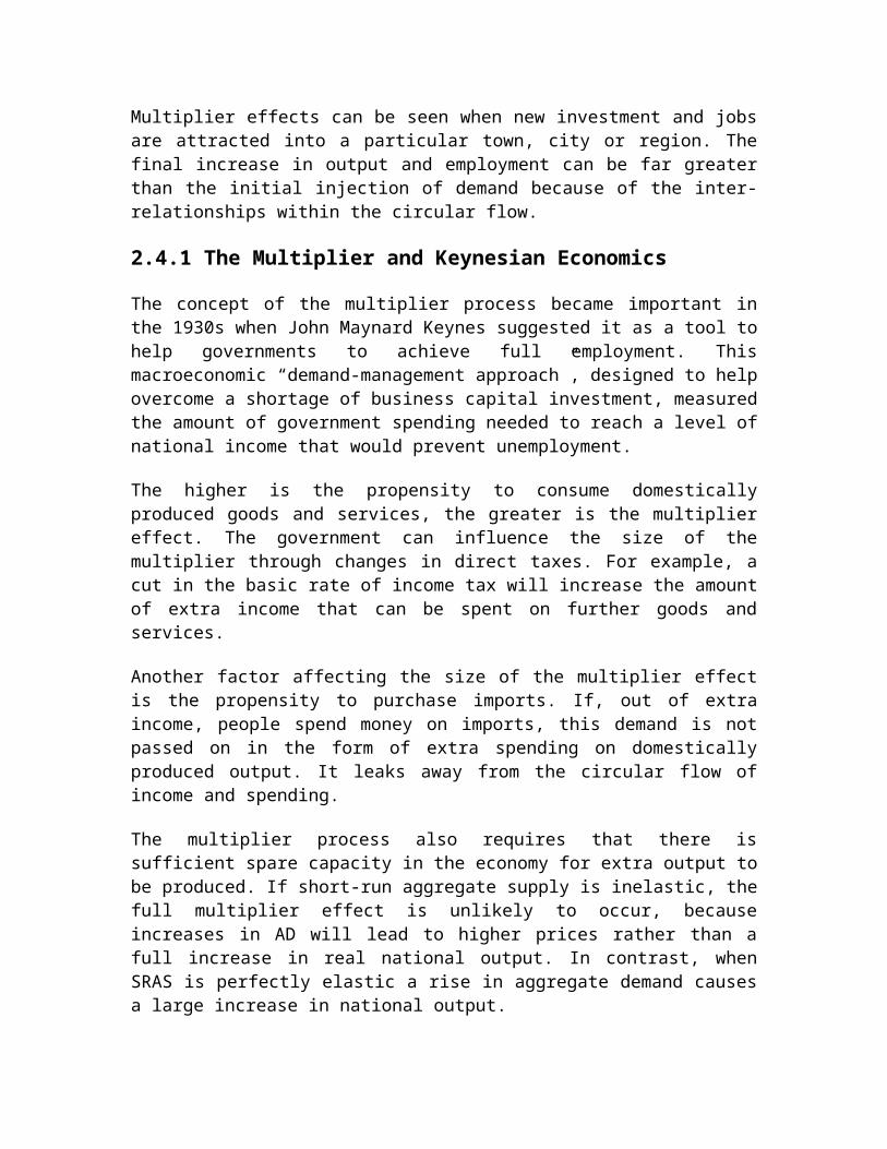
Defining business cycles

In 1946, economists Arthur F. Burns and Wesley C. Mitchell provided the now standard definition of business cycles in their book Measuring Business Cycles:

Business cycles are a type of fluctuation found in the aggregate economic activity of nations that organize their work mainly in business enterprises: a cycle consists of expansions occurring at about the same time in many economic activities, followed by similarly general recessions, contractions, and revivals which merge into the expansion phase of the next cycle; in duration, business cycles vary from more than one year to ten or twelve years; they are not divisible into shorter cycles of similar characteristics with amplitudes approximating their own.

According to A. F. Burns:

Business cycles are not merely fluctuations in aggregate economic activity. The critical feature that distinguishes them from the commercial convulsions of earlier centuries, or from the seasonal and other short term variations of our own age is that the fluctuations are widely diffused over the economy--its industry, its commercial dealings, and its tangles of finance. The economy of the western world is a system of closely interrelated parts. He who would understand business cycles must master the workings of an economic system organized largely in a network of free enterprises searching for profit. The problem of how business cycles come about is therefore inseparable from the problem of how a capitalist economy functions.

In the United States, it is generally accepted that the National Bureau of Economic Research (NBER) is the final arbiter of the dates of the peaks and troughs of the business cycle. An expansion is the period from a trough to a peak, and a recession as the period from a peak to a trough. The NBER identifies a recession as "a significant decline in economic activity spread across the economy, lasting more than a few months, normally visible in real GDP, real income, employment, industrial production".

Cycles or fluctuations?

In recent years economic theory has moved towards the study of economic fluctuation rather than a 'business cycle' - though some economists use the phrase 'business cycle' as a convenient shorthand. For Milton Friedman calling the business cycle a "cycle" is a misnomer, because of its non-cyclical nature. Friedman believed that for the most part, excluding very large supply shocks, business declines are more of a monetary phenomenon.

Rational expectations theory states that no deterministic cycle can persist because it would consistently create arbitrage opportunities. Much economic theory also holds that the economy is usually at or close to equilibrium. These views led to the formulation of the idea that observed economic fluctuations can be modeled as shocks to a system.

In the tradition of Slutsky, business cycles can be viewed as the result of stochastic shocks that on aggregate form a moving average series. However, the recent research employing spectral analysis has confirmed the presence of business (Juglar) cycles in the world GDP dynamics at an acceptable level of statictical significance.

3.2 APPROACHES TO BUSINESS CYCLES

The explanation of fluctuations in aggregate economic activity is one of the primary concerns of macroeconomics. The most commonly used framework for explaining such fluctuations is Keynesian economics. In the Keynesian view, business cycles reflect the possibility that the economy may reach short-run equilibrium at levels below or above full employment. If the economy is operating with less than full employment, i.e., with high unemployment, Keynesian theory states that monetary policy and fiscal policy can have a positive role to play in smoothing the fluctuations of the business cycle.

There are a number of alternative heterodox economic theories of business cycles, largely associated with particular schools or theorists. There are also some divisions and alternative theories within mainstream economics, notably Real Business Cycle theory and credit-based explanations such as debt deflation and the Financial Instability Hypothesis.

3.2.1 Exogenous vs. endogenous

Within mainstream economics, the debate over external (exogenous) versus internal (endogenous) causes of the economic cycle is centuries long, with the classical school (now neo-classical) arguing for exogenous causes and the underconsumptionist (now Keynesian) school arguing for endogenous causes. These may also broadly be classed as "supply-side" and "demand-side" explanations: supply-side explanations may be styled, following Say's law, as arguing that "supply creates its own demand", while demand-side explanations argue that effective demand may fall short of supply, yielding a recession or depression.

This debate has important policy consequences: proponents of exogenous causes of crises such as neoclassicals largely argue for minimal government policy or regulation (laissez faire), as absent these external shocks, the market functions, while proponents of endogenous causes of crises such as Keynesians largely argue for larger government policy and regulation, as absent regulation, the market will move from crisis to crisis. This division is not absolute – some classicals (including Say) argued for government policy to mitigate the damage of economic cycles, despite believing in external causes, while Austrian School economists argue against government involvement as only worsening crises, despite believing in internal causes.

The view of the economic cycle as caused exogenously dates to Say's law, and much debate on endogeneity or exogeneity of causes of the economic cycle is framed in terms of refuting or supporting Say's law; this is also referred to as the "general glut" debate.

Until the Keynesian revolution in mainstream economics in the wake of the Great Depression, classical and neoclassical explanations (exogenous causes) were the mainstream explanation of economic cycles; following the Keynesian revolution, neoclassical macroeconomics was largely rejected. There has been some resurgence of neoclassical approaches in the form of RBC theory, but the mainstream view is largely Keynesian.

Mainstream economists working in the neoclassical tradition of Adam Smith and David Ricardo, as opposed to the Keynesian tradition, have usually viewed the departures of the harmonic working of the market economy as due to exogenous influences, such as the State or its regulations, labor unions, business monopolies, or shocks due to technology or natural causes (e.g. sunspots for William Stanley Jevons, planet Venus movements for Henry Ludwell Moore).

Contrarily, in the heterodox tradition of Jean Charles Léonard de Sismondi, Clement Juglar, and Marx the recurrent upturns and downturns of the market system are an endogenous characteristic of it.

The 19th century school of Underconsumptionism also posited endogenous causes for the business cycle, notably the paradox of thrift, and today this previously heterodox school has entered the mainstream in the form of Keynesian economics via the Keynesian revolution.

3.2.2 Keynesian

According to Keynesian economics, fluctuations in aggregate demand cause the economy to come to short run equilibrium at levels that are different from the full employment rate of output. These fluctuations express themselves as the observed business cycles. Keynesian models do not necessarily imply periodic business cycles. However, simple Keynesian models involving the interaction of the Keynesian multiplier and accelerator give rise to cyclical responses to initial shocks. Paul Samuelson's "oscillator model" is supposed to account for business cycles thanks to the multiplier and the accelerator. The amplitude of the variations in economic output depends on the level of the investment, for investment determines the level of aggregate output (multiplier), and is determined by aggregate demand (accelerator).

In the Keynesian tradition, Richard Goodwin accounts for cycles in output by the distribution of income between business profits and workers wages. The fluctuations in wages are almost the same as in the level of employment (wage cycle lags one period behind the employment cycle), for when the economy is at high employment, workers are able to demand rises in wages, whereas in periods of high unemployment, wages tend to fall. According to Goodwin, when unemployment and business profits rise, the output rises.

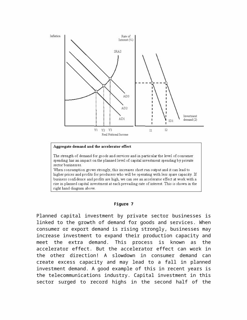
3.2.3 Credit/debt cycle

One alternative theory is that the primary cause of economic cycles is due to the credit cycle: the net expansion of credit (increase in private credit, equivalently debt, as a percentage of GDP) yields economic expansions, while the net contraction causes recessions, and if it persists, depressions. In particular, the bursting of speculative bubbles is seen as the proximate cause of depressions, and this theory places finance and banks at the center of the business cycle.

A primary theory in this vein is the debt deflation theory of Irving Fisher, which he proposed to explain the Great Depression. A more recent complementary theory is the Financial Instability Hypothesis of Hyman Minsky, and the credit theory of economic cycles is often associated with Post-Keynesian economics such as Steve Keen.

Post-Keynesian economist Hyman Minsky has proposed a explanation of cycles founded on fluctuations in credit, interest rates and financial frailty, called the Financial Instability Hypothesis. In an expansion period, interest rates are low and companies easily borrow money from banks to invest. Banks are not reluctant to grant them loans, because expanding economic activity allows business increasing cash flows and therefore they will be able to easily pay back the loans. This process leads to firms becoming excessively indebted, so that they stop investing, and the economy goes into recession.

While credit causes have not been a primary theory of the economic cycle within the mainstream, they have gained occasional mention, such as (Eckstein & Sinai 1986), cited approvingly by (Summers 1986).

3.2.4 Real business cycle theory

Within mainstream economics, Keynesian views have been challenged by real business cycle models in which fluctuations are due to technology shocks. This theory is most associated with Finn E. Kydland and Edward C. Prescott, and more generally the Chicago school of economics (freshwater economics). They consider that economic crisis and fluctuations cannot stem from a monetary shock, only from an external shock, such as an innovation.

RBC theory has been categorically rejected by a number of mainstream economists in the Keynesian tradition, such as (Summers 1986) and Paul Krugman.

3.2.5 Politically-based business cycle

Another set of models tries to derive the business cycle from political decisions. The partisan business cycle suggests that cycles result from the successive elections of administrations with different policy regimes. Regime A adopts expansionary policies, resulting in growth and inflation, but is voted out of office when inflation becomes unacceptably high. The replacement, Regime B, adopts contractionary policies reducing

inflation and growth, and the downwards swing of the cycle. It is voted out of office when unemployment is too high, being replaced by Party A.

The political business cycle is an alternative theory stating that when an administration of any hue is elected, it initially adopts a contractionary policy to reduce inflation and gain a reputation for economic competence. It then adopts an expansionary policy in the lead up to the next election, hoping to achieve simultaneously low inflation and unemployment on Election Day.

The political business cycle theory is strongly linked to the name of Michał Kalecki who argued that no democratic government under capitalism would allow the persistence of full employment, so that recessions would be caused by political decisions. Persistent full employment would mean increasing workers' bargaining power to raise wages and to avoid doing unpaid labor, potentially hurting profitability. (He did not see this theory as applying under fascism, which would use direct force to destroy labor's power.) In recent years, proponents of the "electoral business cycle" theory have argued that incumbent politicians encourage prosperity before elections in order to ensure re-election—and make the citizens pay for it with recessions afterwards.

3.2.6 Marxian economics

For Marx the economy based on production of commodities to be sold in the market is intrinsically prone to crisis. In the Marxian view profit is the major engine of the market economy, but business (capital) profitability has a tendency to fall that recurrently creates crises, in which mass unemployment occurs, businesses fail, remaining capital is centralized and concentrated and profitability is recovered. In the long run these crises tend to be more severe and the system will eventually fail. Some Marxist authors such as Rosa Luxemburg viewed the lack of purchasing power of workers as a cause of a tendency of supply to be larger than demand, creating crisis, in a model that has similarities with the Keynesian one. Indeed a number of modern authors have tried to combine Marx's and Keynes's views. Others have contrarily emphasized basic differences between the Marxian and the Keynesian perspective: while Keynes saw capitalism as a system worth maintaining and susceptible to efficient regulation, Marx viewed capitalism as a historically doomed system that cannot be put under societal control

3.2.7 Austrian school

Economists of the Austrian school argue that business cycles are caused by monetary expansion, which is often created by central banks and fractional reserve banks in modern economies. Austrian business cycle theory, following the work of Ludwig von Mises and Friedrich Hayek, points to the role of the interest rates as the price of investment capital, guiding investment decisions. They argue that in an unregulated (free-market) economy, without a central bank, interest rates reflect the actual time preference of lenders and borrowers. Some follow Knut Wicksell in calling this the "natural" interest rate. Austrian school economists argue that a central bank distorts this natural equilibrium. If the interest rate is held artificially low by the government or central bank, then the demand

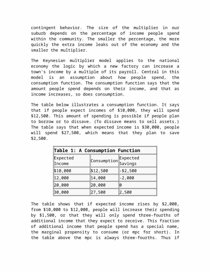
for loans will exceed the supply of willing lenders, and if the interest rate is artificially high, the opposite will occur. This pricing misinformation leads investors to misallocate capital, borrowing and investing either too much when interest rates are too low or too little when the rates are too high, in long-term projects. Periodic recessions are seen as necessary "corrections" following periods of monetary expansion, when unprofitable investments are liquidated, freeing capital for new investment. Depressions and recessions are positive forces in-so-much that they are the market's natural mechanism of undoing the misallocation of resources present during the “boom” or inflationary phase.

There are various critiques of Austrian business cycle theory, not least of which that the US suffered recurrent economic crises in the 19th century, most notably the Long Depression following the Panic of 1873, prior to the establishment of a US central bank in 1907. The historian Thomas Woods has attempted to explain that these earlier financial crises are in fact consistent with Austrian theory in his book Meltdown.

3.2.8 Mitigating

Most social indicators (mental health, crimes, suicides) worsen during economic recessions. As periods of economic stagnation are painful for the many who lose their jobs, there is often political pressure for governments to mitigate recessions. Since the 1940s, most governments of developed nations have seen the mitigation of the business cycle as part of the responsibility of government.

Since in the Keynesian view, recessions are caused by inadequate aggregate demand, when a recession occurs the government should increase the amount of aggregate demand and bring the economy back into equilibrium. This the government can do in two ways, firstly by increasing the money supply (expansionary monetary policy) and secondly by increasing government spending or cutting taxes (expansionary fiscal policy).

However, even according to Keynesian theory, managing economic policy to smooth out the cycle is a difficult task in a society with a complex economy. Some theorists, notably those who believe in Marxian economics, believe that this difficulty is insurmountable. Karl Marx claimed that recurrent business cycle crises were an inevitable result of the operations of the capitalistic system. In this view, all that the government can do is to change the timing of economic crises. The crisis could also show up in a different form, for example as severe inflation or a steadily increasing government deficit. Worse, by delaying a crisis, government policy is seen as making it more dramatic and thus more painful.

Additionally, since the 1960s neoclassical economists have played down the ability of Keynesian policies to manage an economy. Since the 1960s, economists like Nobel Laureates Milton Friedman and Edmund Phelps have made ground in their arguments that inflationary expectations negate the Phillips curve in the long run. The stagflation of the 1970s provided striking support for their theories, defying the simple Keynesian prediction that recessions and inflation cannot occur together. Friedman has gone so far as to argue that all the central bank of a country should do is to avoid making large

mistakes, as he believes they did by contracting the money supply very rapidly in the face of the Wall Street Crash of 1929, in which they made what would have been a recession into the Great Depression.

3.3 SCHUMPETER AND BUSINESS CYCLES

Joseph Alois Schumpeter (8 February 1883 – 8 January 1950) was an economist and political scientist born in Moravia, then Austria-Hungary, now Czech Republic. He popularized the term "creative destruction" in economics

The leading economic theoretician to work on trade cycles in the first half of the twentieth century was undoubtedly Joseph Schumpeter. He was an Austrian, but cannot properly be regarded as a member of the Austrian School. He is not a liberal economist like von Hayek or von Mises. Joseph Schumpeter can properly be regarded as a man of the left, though certainly not of the far left. In 1927, Schumpeter published in Economica his paper on” The explanation of the business cycle”. After the global shock of the banking crisis of 2008, which itself came more than eighty years after this paper was published, the world is again looking for explanations.

Schumpeter is important because he developed a theory of business cycles which puts its emphasis on industrial innovations rather than banking. Most business cycle theories put their emphasis the other way, and are essentially monetary. Maynard Keynes is just as much a monetary economist as Milton Friedman when he comes to his explanation of business cycles. This is surely an argument which is going to be reopened.

Schumpeter starts his account of business cycles at the top rather than the bottom of the cycle. “These booms consist in the carrying out of innovations in the industrial and commercial organisms. By innovations I understand such changes in the combinations of the factors of production as cannot be effected by infinitesimal steps or variations on the margin. They consist primarily in changes of methods of production and transportation, or in changes of industrial organisation, or in the production of a new article, or in the opening up of new markets or of new sources of material. The recurring periods of prosperity of the cyclical movements are the form progress takes in a capitalist society.”

He goes on to argue from economic history – and this part of the Schumpeter argument would be difficult to question. “The reader needs only to make the experiment. If he comes to survey industrial history from, say, 1760 onwards, he will discover two things; he will find that very many booms are unmistakably characterised by revolutionary changes in some branch of industry which, in consequence, leads the boom, railways, for instance in the forties, or steel in the eighties, or electricity in the nineties…”

His conclusion is stated very clearly: “booms and consequently depressions are not the work of banks: their cause is a non-monetary one and entrepreneurs demand is the initialing cause even of so much of the cycle as can be said to be added by the act of banks.”

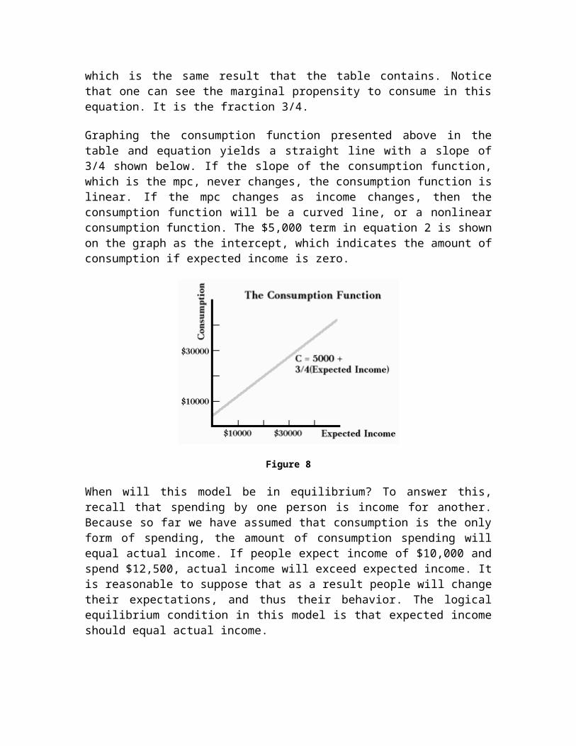
In 2008, we have had a conspicuous example of a crash apparently caused by the banks. It looks like the “debt-deflation” type of crash. But we also have to account for oil, for Google, for China. These are the triggers which may be the underlying explanation of the behaviour of the banks. The relationship between business cycles and changes in business conditions may be mediated through bankers or speculators, but the big causes, as Schumpeter believed, may not lie in the banks themselves.

Schumpeter's relationships with the ideas of other economists were quite complex in his most important contributions to economic analysis - the theory of business cycles and development. Following neither Walras nor Keynes, Schumpeter starts in The Theory of Economic Development with a treatise of circular flow which, excluding any innovations and innovative activities, leads to a stationary state. The stationary state is, according to Schumpeter, described by Walrasian equilibrium. The hero of his story, though, is, in fine Austrian fashion, the entrepreneur.

The entrepreneur disturbs this equilibrium and is the prime cause of economic development, which proceeds in cyclic fashion along several time scales. In fashioning this theory connecting innovations, cycles, and development, Schumpeter kept alive the Russian Nikolai Kondratiev's ideas on 50-year cycles, Kondratiev waves.

Schumpeter suggested a model in which the four main cycles, Kondratiev (54 years), Kuznets (18 years), Juglar (9 years) and Kitchin (about 4 years) can be added together to form a composite waveform. (Actually there was considerable professional rivalry between Schumpeter and Kuznets. The wave form suggested here did not include the Kuznets Cycle simply because Schumpeter did not recognize it as a valid cycle. See "Business Cycle" for further information.) A Kondratiev wave could consist of three lower degree Kuznets waves. Each Kuznets wave could, itself, be made up of two Juglar waves. Similarly two (or three) Kitchin waves could form a higher degree Juglar wave. If each of these were in phase, more importantly if the downward arc of each was simultaneous so that the nadir of each was coincident it would explain disastrous slumps and consequent depressions. (As far as the segmentation of the Kondratyev Wave, Schumpeter never proposed such a fixed model. He saw these cycles varying in time - although in a tight time frame by coincidence - and for each to serve a specific purpose)

Schumpeter and Keynesianism

Unlike Keynes, in Schumpeter's theory, Walrasian equilibrium is not adequate to capture the key mechanisms of economic development. Schumpeter also thought that the institution enabling the entrepreneur to purchase the resources needed to realize his or her vision was a well-developed capitalist financial system, including a whole range of institutions for granting credit. One could divide economists among (1) those who emphasized "real" analysis and regarded money as merely a "veil" and (2) those who thought monetary institutions are important and money could be a separate driving force. Both Schumpeter and Keynes were among the latter. Nevertheless, Schumpeter, who was a classical liberal, rejected Keynesianism

3.4 KALDOR'S NON-LINEAR CYCLE

One of the most interesting theories of business cycles in the Keynesian vein is that expounded in a pioneering article by Nicholas Kaldor (1940). It is distinguishable from most other contemporary treatments since it utilizes non-linear functions, which produce endogenous cycles, rather than the linear multiplier-accelerator kind which rely largely on exogenous factors to maintain regular cycles. We shall follow Kaldor's simple argument and then proceed to analyze Kaldor in the light of the rigorous treatment given to it by Chang and Smyth (1971) and Varian (1979).

What prompted Kaldor's innovation? Besides the influence of Keynes (1936) and Kalecki (1937), in his extremely readable article, Kaldor proposed that the treatment of savings and investment as linear curves simply does not correspond to empirical reality. In (Harrodian version of) Keynesian theory, investment and savings are both positive functions of output (income). The savings relationship is cemented by the income-expenditure theory of Keynes:

S = (1-c)Y

whereas investment is positively related to income via an accelerator-like relationship, (which, in Kaldor, is related to the level rather than the change in income):

I = vY

where v, the Harrod-Kaldor accelerator coefficient, is merely the capital-output ratio. Over these two relationships, Kaldor superimposed Keynes's multiplier theory: namely, that output changes to clear the goods market. Thus, if there is excess goods demand (which translates to saying that investment exceeds savings, I > S), then output rises (dY/dt > 0), whereas if there is excess goods supply (which translates to savings exceeding investment, I < S), then output falls.

The implications of linearity can be visualized in Figure 1, where we draw two positively-sloped linear I and S curves. To economize on space, we place two separate sets of curves in the same diagram. In the left part of Figure 1, the slope of the savings function is larger than that of the investment function. Where they intersect (I = S) is the equilibrium Y*. As we can note, left of Y*, investment is greater than savings (I > S), hence output will increase by the multiplier dynamic. Right of point Y*, savings is greater than investment (I < S), hence output will fall. Thus, the equilibrium point Y* is stable.

In the right side of Figure 1, we see linear S and I functions again, but this time, the slope of the investment curve is greater than that of the savings curve. Where they intersect, Y*, investment equals savings (I = S) and we have equilibrium. However, note that left of the equilibrium Y*, savings are greater than investment (I < S), thus output will contract and we will move away from Y*. In contrast, right of Y*, investment is greater than

savings (I > S), so output will increase and move further to the right of Y*. Thus, equilibrium Y* is unstable.

Fig. 1 - Savings, Investment and Output Adjustment

Both exclusive cases, complete stability and complete instability, are implied by linear I and S curves in figure 1, are incompatible with the empirical reality of cycles and fluctuations. Hence, Kaldor concluded, it might be sensible to assume that the S and I curves are non-linear. In general, he assumed I = I(Y, K) and S = S(Y, K), where investment and savings are non-linear functions of income and capital as in the Figure 2 below.

We shall focus the relationship with income first. The logic Kaldor (1940) gave for this is quite simple. The non-linear investment curve, shown in Figure 2 can be explained by simply recognizing that the rate of investment will be quite low at extreme output levels. Why? Well, at low output levels (e.g. at YA), there is so much excess capacity that any increase in aggregate demand will induce very little extra investment. The extra demand can be accomodated by existing capacity, so the rate of investment is low. In contrast, at high rates of output, such as YC, Wicksellian problems set in. In other words, with such high levels of output and demand, the cost of expanding capacity is also increasing, capital goods industries are supply-constrained and thus demand a higher price from entrepreneurs for producing an extra unit of capital. In addition, the best investment projects have probably all already been undertaken at this point, so that the only projects left are low-yielding and simply might not be worth the effort for the entrepreneur. Thus, the rate of investment will also be relatively low. At output levels between YA and YC

(e.g. at YB), the rate of investment is higher. Thus, the non-linearity of the I curve is reasonably justified.

What about the non-linear savings curve, S? As shown in Figure 2, it is assumed by Kaldor that savings rates are high at extreme levels of output. At low levels of output (YA), income is so low that savings are the first to be cut by individuals in their household decisions. Therefore, at this point, the rate of saving (or rather, in this context, the rate of dissaving) is extremely high. Slight improvements in income, however, are not all consumed (perhaps by custom or precaution), but rather much of it is saved. In contrast, at high levels of output, YC, income is so high that the consumer is effectively saturated. Consequently, he will save a far greater portion of his income - thus, at points like YC, the savings rate is quite high.

Fig. 2 - Non-Linear Investment and Savings

With the non-linearity of I and S justified, Kaldor (1940) proceeded to analyze cyclical behavior by superimposing the I and S curves (as in Figure 2). As we can see, there are three points of intersection (A, B and C) where savings equals investment (I = S). Let us consider each individually. Left of point A, investment is greater than savings hence, by the multiplier, Y increases to YA; to the right of point A, savings is greater than investment (hence Y decreases to YA). Consequently, it is easy to note that A (and YA) is a stable point. The same analysis applies to the points to the right and left of YC, hence C (and YC) is also a stable point.

Intersection point B (at YB) in Figure 2 is the odd one. Left of B, savings exceeds investment (so Y falls left of YB) and right of B, investment exceeds savings (so Y increases right of YB). Thus, B is an unstable point. Consequently, then, we are faced with two stable equilibria (A and C) and an unstable equilibrium (B). How can this explain cyclical phenomenon? If we are at A, we stay at A. If we are at C, we stay at C. If we are at B, we will move either to A or C with a slight displacement. However, no cycles are apparent.

The clincher in Kaldor's system is the phenomenon of capital accumulation at a given point in time. After all, as Kaldor reminds us, investment and savings functions are short term. At a high stable level of output, such as that at point YC in the figure above, if investment is happening, the stock of capital is increasing. As capital stock increases, there are some substantial changes in the I and S curves. In the first instance, as capital stock increases, the return or marginal productivity of capital declines. Thus, it is not unreasonable to assume that investment will fall over time. Thus, it is acceptable that dI/dK < 0, i.e. the I curve falls.

However, as capital goods become more available, a greater proportion of production can be dedicated to the production of consumer goods. As consumer goods themselves increase in number, the prices of consumer goods decline. For the individual consumer, this phenomenon is significant since it implies that less income is required to purchase the same amount of goods as before. Consequently, there will be more income left over to be saved. Thus, it is also not unreasonable to suspect that the savings curve, S, will gradually move upwards, i.e. dS/dK > 0. This is illustrated in Figure 3.

 

Fig. 3 - Capital Accumulation and Gravitation of Investment and Savings Curves

So, we can see the story by visualizing the move from Figure 2 to Figure 3.  Starting from our (old)YC, as I(Y, K) moves down and S(Y, K) moves down, point B will gradually move from its original position in the middle towards C (i.e. YB will move right) while point C moves towards B (YC moves left). As shown in Figure 3, as time progresses, and the investment and savings curves continue on their migration induced by capital accumulation, and B and C approximate each other, we will reach a situation where B and C meet at YB = YB and the S and I curves are tangential to each other. Notice that at this point in time, C is no longer stable - left and right of point C, savings exceeds

investment, thus output must fall - and indeed will fall catastrophically from YB = YC to the only stable point in the system: namely, point A at YA.

At YA, we are again at a stable, short-run equilibrium. However, as in the earlier case, the S and I curves are not going to remain unchanged. In fact, they will move in the opposite direction. As investment is reined back, there might not even be enough to cover replacement. Thus, previous investment projects which were running on existing capital will disappear with depreciation. The usefulness (i.e. productivity) of the projects, however, remains. Thus, the projects reemerge as "new" opportunities. In simplest terms, with capital decumulation, the return to capital increases and hence investment becomes more attractive, so that the I curve will shift upwards (see Figure 4). Similarly, as capital is decumulated, consumer industries will disappear, prices rise and hence real income (purchasing power) per head declines so that, to keep a given level of real consumption, savings must decline. So, the S curve falls. Ultimately, as time progresses and the curves keep shifting, as shown in Figure 4, until we will reach another tangency between S and I analogous to the one before. Here, points B and A merge at YA = YB and the system becomes unstable so that the only stable point left is C. Hence, there will be a catastrophic rise in production from YA to YC.

Fig. 4 - Capital Decumulation and Gravitation

Thus, we can begin to see some cyclical phenomenon in action. YA and YC are both short-term equilibrium levels of output. However, neither of them, in the long-term, is stable. Consequently, as time progresses, we will be alternating between output levels near the lower end (around YA) and output levels near the higher end (around YC). Moving from YA to YC and back to YA and so on is an inexorable phenomenon. In simplest terms, it is Kaldor's trade cycle.

W.W. Chang and D.J. Smyth (1971) and Hal Varian (1979) translated Kaldor's trade cycle model into more rigorous context: the former into a limit cycle and the latter into catastrophe theory. Output, as we saw via the theory of the multiplier , responds to the difference between savings and investment. Thus:

dY/dt = x (I - S)

where x is the "speed" by which output responds to excess investment. If I > S, dY/dt > 0. If I < S, dY/dt < 0. Now both savings and investment are positive (non-linear) functions of income and capital, hence I = I(K, Y) and S = S(K, Y) where dI/dY= I Y > 0 and dS/dY = SY > 0 while dI/dK = IK < 0 and dS/dK = SK > 0, for the reasons explained before. At any of the three intersection points, YA, YB and YC, savings are equal to investment (I - S = 0).

We are faced basically with two differential equations:

dY/dt = x [I(K,Y) - S(K,Y)]

dK/dt = I(K, Y)

To examine the local dynamics, let us linearize these equations around an equilibrium (Y*, K*) and restate them in a matrix system:

dY/dt x (IY - SY) x (IK - SK) Y= 

dK/dt  IY  IK  [Y*, K*] K

the Jacobian matrix of first derivatives evaluated locally at equilibrium (Y*, K*), call it A, has determinant:

|A| = x (IY - SY)IK - x (IK - SK)IY

= x (SKIY - IKSY)

where, since IK < 0 and SK, SY, IY > 0 then |A| > 0, thus we have regular (non-saddlepoint) dynamics. To examine local stability, the trace is simply:

tr A = x (IY - SY) + IK

whose sign, obviously, will depend upon the sign of (IY - SY). Now, examine the earlier Figures 3 and 4 again. Notice around the extreme areas, i.e. around YA and YC, the slope of the savings function is greater than the slope of the investment function, i.e. dS/dY > dI/dY or, in other words, IY - SY < 0. In contrast, around the middle areas (around YB) the slope of the savings function is less than the slope of the investment function, thus IY - SY

> 0. Thus, assuming Ik is sufficiently small, the trace of the matrix will be positive around

the middle area (around YB), thus equilibrium B is locally unstable, whereas around the extremes (YA and YC), the trace will be negative, thus equilibrium A and C are locally stable. This is as we expected from the earlier diagrams.

To obtain the phase diagram in Figure 5, we must obtain the isoclines dY/dt = 0 and dK/dt = 0 by evaluating each differential equation at steady state. When dY/dt = 0, note that x [I(Y, K) - S(Y, K)] = 0, then using the implicit function theorem:

dK/dY|dY/dt = 0 = -(IY - SY)/(IK - SK)

Now, we know from before that Ik < 0 and Sk > 0, thus the denominator (Ik - Sk) < 0 for certain. The shape of the isocline for dY/dt = 0, thus, depends upon the value of (Iy - Sy). As we claimed earlier, for extreme values of Y (around YA and YC), we had (IY - Sy) < 0, thus dK/dY|Y < 0, i.e. the isocline is negatively shaped. However, around middle values of Y (around YB), we had (IY - SY) > 0, thus dK/dY|Y > 0, i.e. the isocline is positively shaped. This is shown in Figure 5.

 

Fig. 5 - Isokine for dY/dt = 0

From Figure 5, we see that at low values of Y (below Y1) and high values of Y (above Y2), the isokine is negatively-sloped - this corresponds to the areas in our earlier diagrams where the savings function was steeper than the investment function (e.g. around YA and YC). However, between Y1 and Y2, the isokine is positively-sloped - which corresponds to the areas where investment is steeper than savings (around YB in our earlier diagrams). The off-isokine dynamics are easy, namely differentiating the differential equation dY/dt for K:

d(dY/dt)/dK = x [IK - SK] < 0

as IK < 0 and SK > 0. Thus, above the isokine, dY/dt < 0, so output falls whereas below the isokine, dY/dt > 0, so output rises. The directional arrows indicate these tendencies.

We can already get a flavor of Kaldor's trade cycle from Figure 6. Remember that our earlier Kaldorian diagrams were drawn for a particular level of capital, K. Thus, as we see in Figure 6, for a given level of K0, we can find the corresponding equilibria (YA, YB, YC) at the intersection between the isokine and the level line K0. However, suppose we start at point C so that K begins to rise: notice that when K0 rises to K2, the points YC and YB begin to move together and finally "merge" at the critical point D (which corresponds to our old B=C) at point Y2. The underlying dynamic (represented by the phase arrows) implies that point D is completely unstable so there will be a catastrophic jump from D to the lower equilibrium E (which is where A moved to as K rose from K0 to K2). Notice that during this catastrophic fall in output is driven solely by the fast multiplier dynamic - the slower-moving capital dynamic is inoperative as, in moving from D to E, capital is constant at K2.

Figure 6 - Dynamics of the Kaldor Cycle

The rest of the story then follows in reverse. At E in Figure 6, we are at a pretty low output level and thus capital decumulates and so K declines from K2 past K0 and then on towards K1. In the meantime, our lower two equilibrium begin to move towards each other and A and B meet and merge at point F at Y1 (equivalent to our old A=B). Note that the stability arrows in Figure 6 are such that now we must have a catastrophic jump in output from F to point G (the high equilibrium to which point C moved to as capital fell from K2 to K1). From G, the process then begins again as capital rises at high output levels from K1 to K0 and onto K2.

The output cycle that can be traced out from the arrows drawn in Figure 6 (from slow movement from G to C to D then catastrophic jump to E then slow movement from E to A to F then catastrophic jump to G, etc.) is Kaldor's trade cycle: output thus fluctuates over time between the boundaries imposed by the extreme points E (lower bound) and G (upper bound). Notice that the cycle is completely endogenous: no exogenous shocks, ceilings, floors, structurally unstable parameter values or ratchets are necessary to obtain constant cycles. The non-linearity of the curves, which are economically-justified and not exceptional, is more than sufficient to generate endogenous cycles.

This version of Kaldor's model is derived a bit more formally in Varian (1979) using catastrophe theory. However, we can also use regular non-linear dynamical theory, which makes no assumptions about the relative speeds of the dynamics, to obtain a cycle from the Kaldor model - and this is what Chang and Smyth (1971) do. We have already derived the isokine dY/dt = 0, so to get the full story, we need the dK/dt = 0 isokine. This is simple. dK/dt = I(Y, K), thus at steady-state, dK/dt = 0 = I(Y, K) so the isokine has slope:

dK/dY|K = -IY/IK > 0

as IY < 0 and IK > 0. Thus, the dK/dt = 0 isokine is positive sloped. We have superimposed it on the other isokine in Figure 7. For the off-isokine dynamics, note that:

d(dK/dt)/dY = IY > 0

so that the directional arrows drawn in for the dK/dt = 0 isokine imply that to the left of it, dK/dt < 0 (capital falls) whereas to the right, dK/dt > 0 (capital rises). In the figure below, we have superimposed the isokines for the whole system. As is obvious, the global equilibrium, where dK/dt = dY/dt = 0, is at K* and Y* (point E). Now, as we showed earlier, the trace of the system, tr A, is positive around point E, thus we know that the global equilibrium is locally unstable - as is shown in Figure 7 by the unstable trajectory that emerges when we move slightly off the equilibrium point E..

Fig. 7 - Kaldor's Trade Cycle

However, notice that the system as a whole is "stable": when we draw a "box" around the diagram by imposing upper boundaries Km and Ym in Figure 7 and letting the axis act as lower boundaries, then the directional phase arrows around the boundaries of the box indicate that we do not get out of the confines of this box - any trajectory which enters the "box" will not leave it. Indeed, from the distant boundaries, it almost seems as if we are moving towards the global equilibrium (K*, Y*). Thus, while the equilibrium (K*, Y*) is locally unstable, we are still confined within this "box". Note that we are assuming complex roots to obtain stable and unstable focal dynamics as opposed to simply monotonic ones.

In fact, these three conditions - complex roots, locally unstable equilibrium and a "confining box" - are all that is necessary to fulfill the Poincar-Bendixson Theorem on the existence of a dynamic "limit cycle". This limit cycle is shown by the thick black circle in Figure 7 (not perfectly drawn) orbiting around the equilibrium. Any trajectory that begins within the circle created by the limit cycle will be explosive and move out towards the cycle. In contrast, any trajectory that begins outside the circle will be dampened and move in towards it. Two such trajectories are shown in Figure 7. Thus, the limit cycle "attracts" all dynamic trajectories to itself and once trajectory confluences with the limit cycle; it proceeds to follow the orbit of the limit cycle forever (as shown by the directional arrows on the cycle).

3.5 SAMUELSON AND HICKS MODEL

In the Samuelson–Hicks business cycle model, investment is determined by the growth in income, through the principle of acceleration. More precisely, investment is taken to be proportional to the rate of change in income, or It = k(Yt−1 − Yt−2), where It denotes investment in time period t, Yt−1 and Yt−2 income one and two periods back, respectively, and the parameter k (>0) is the accelerator (this parameter is the technical coefficient for capital, it is the volume of capital needed to produce one unit of goods during one time period). In past empirical measurement a realistic estimate was considered to be about 2–4. Obviously, this numerical value depends on the choice of the length of the basic time period for the model.

It is important in this context to realize that economics distinguishes between concepts of stocks and flows. Stocks are variables hich are meaningful by reference to a point of time, such as a stock of capital or the labour force. Flows, on the other hand, are concepts referring to time periods, defined by a beginning and a finishing point on the time scale.

To the flows belong investments, consumption, and income/production. A produced quantity, given inputs in form of capital and labour stocks, obviously depends on the length of the time period. During half the period chosen, output is half, during double the period it double that for a period. In some economic models the period length may be a bit ambiguous. This is, however, not the case in macro economic models, which arose in connection with Keynesian theory and national accounting in the 1930’s. The reference period is always one year, and whenever accounts or forecasts are made for shorter periods, they are always evaluated to a yearly basis.

Hence, the time period in macro economic models such as the present is always the calendar year. As for the consumption function, a Robertsonian formulation is assumed, Ct = bYt−1 where 0 < b < 1 is the marginal propensity to consume (realistic values belongs to the range (0.6, 1)). Any additional constant term is absorbed in the autonomous expenditure term to be introduced below. This is composed of all the expenditures not dependent on the business cycle, i.e. government expenditures, non-induced investments, due to for instance innovations, and any non-income dependent consumption expenditures.

It is common knowledge that consumers need to consume something to survive even if they earn nothing. When population/labour force grows, then the autonomous expenditures for this minimum subsistence consumption must grow along with the labour force. The Keynesian income formation identity Yt = Ct +It , allows us to obtain a simple recurrence relation in the income variable: Yt = (b+k)Yt−1−kYt−2. This has a closed form solution and models the business cycles mechanism. The solution is the product of an exponential growth, or decline factor, and, in case of complex roots to the characteristic equation, a harmonically varying cyclic function.

The cyclical element provides a possibility for explaining recurrent cycles, but the exponential factor poses a problem. As it is an unlikely coincidence for the exponential factor to become a constant, the cycles are either exponentially increasing or decreasing in amplitude. If they are decreasing, there is no dynamic theory at all, because the theory

only explains how the system goes to eternal equilibrium suggests that external shocks have to be introduced to keep an oscillating system going, even when it is damped. The dynamical system itself would then provide for a periodicity.

Hicks choose another possibility: to introduce bounds for the linear accelerator. At the same time tries to model a growth process within the Keynesian tradition. As it is well known, the Harrodian equilibrium growth path is unstable, and so is the business cycles mechanism in the empirically relevant parameters space of the multiplier-accelerator mechanism. Hicks therefore develop a Harrodian multiplier-accelerator framework with ceilings and floors, thereby constraining the instability problems and producing cyclical behaviour (technically he moves from a linear to a piecewise-linear system). According to Hicks, when income decreases with fixed proportions technology, more capital could be dispensed with than normally what disappears during one period through natural wear. As the capitalists are assumed not actively to destroy capital, just abstain from reinvesting, there is a lower bound to disinvestments, the floor (i.e. net investment cannot be negative).

Likewise, if income is rising, other factors of production, labour force or raw materials, become limiting, then there would be no point in pushing investment any further, so there is also a ceiling to investments (full employment, e.g.). Accordingly, a lower and an upper bound to investment limit the action of the linear acceleration principle. This in fact makes the investment function piecewise-linear, i.e. nonlinear. The result could be self-sustained oscillations of limited amplitude. In his book, Hicks introduces autonomous expenditures which are not constant, but may be growing exponentially, i.e. At = A0(1+g)t , where g isa given growth rate and A0 a positive constant. Summarizing we have:

So, the Schumpeter and Hicks model predicted that an increase in government spending would cause GDP to expand. However, when the government needs more money, it drives up interest rates. This is bad for the private sector, which can have its investments crowded out. The level of decrease in private investment was unclear. Maybe Samuelson and other policy makers thought that government spending should fill in when private investment fell short in order to straighten total investment, which in turn determines GDP. That way, they might have hoped, business cycles might go away

3.6 IMPLICATION OF POLICIES AND CONTROL OF BUSINESS CYCLES

Market economies have regular fluctuations in the level of economic activity which we call the business cycle. It is convenient to think of the business cycle as having three phases. The first phase is expansion when the economy is growing along its long term trends in employment, output, and income. But at some point the economy will overheat, and suffer rising prices and interest rates, until it reaches a turning point -- a peak -- and turn downward into a recession (the second phase). Recessions are usually brief (six to nine months) and are marked by falling employment, output, income, prices, and interest rates. Most significantly, recessions are marked by rising unemployment. The economy will hit a bottom point -- a trough -- and rebound into a strong recovery (the third phase). The recovery will enjoy rising employment, output, and income while unemployment will fall. The recovery will gradually slow down as the economy once again assumes its long term growth trends, and the recovery will transform into an expansion.

3.6.1 Economic policy and the business cycle

The approach to the business cycle depends upon the type of economic system. Under a communist system, there is no business cycle since all economic activities are controlled by the central planners. Indeed, this lack of a business cycle is often cited as an advantage of a command economy. Both socialist and fascist economies have a mix of market and command sectors. Again, the command sector in these economies will not have a business cycle -- while the market sector will display a cyclical activity. In a full market economy -- like the United States -- the nation can suffer extreme swings in the level of economic activity.

The economic policies used by the government to smooth out the extreme swings of the business cycle are called contracyclical or stabilization policies, and are based on the theories of John Maynard Keynes. Writing in 1936 (the Great Depression), Keynes argued that the business cycle was due to extreme swings in the total demand for goods and services. The total demand in an economy from households, business, and government is called aggregate demand. Contracyclical policy is increasing aggregate demand in recessions and decreasing aggregate demand in overheated expansions.

In a market economy (or market sector) the government has two types of economic policies to control aggregate demand -- fiscal policy and monetary policy. When these policies are used to stimulate the economy during a recession, it is said that the government is pursuing expansionary economic policies. And when they are used to contract the economy during an overheated expansion, it is said that the government is pursuing contractionary economic policies.

3.6.2 Other policies

1) Discretionary Fiscal Policy. Fiscal policy is changes in the taxing and spending of the federal government for purposes of expanding or contracting the level of aggregate demand. In recession, an expansionary fiscal policy involves lowering taxes and increasing government spending. In an overheated expansion, a contractionary fiscal policy requires higher taxes and reduced spending.

The first way this can be done is through the federal budget process. However, this process takes so long -- 12 to 18 months -- that discretionary fiscal policy cannot be matched with the business cycle. The Kennedy tax cut of 1964 and later the Ford tax increase of 1974 hit the economy just when the opposite contra cyclical policy was needed. As a result, the federal government no longer uses discretionary fiscal policy.

2) Automatic Stabilizers. A second type of fiscal policy is built into the structure of federal taxes and spending. This is referred to as "nondiscretionary fiscal policy" or more commonly as "automatic stabilizers". The progressive income tax (the major source of federal revenue) and the welfare system both act to increase aggregate demand in recessions and to decrease aggregate demand in overheated expansions.

3) Monetary Policy. Monetary policy is under the control of the Federal Reserve System (our central bank) and is completely discretionary. It is the changes in interest rates and money supply to expand or contract aggregate demand. In a recession, the Fed will lower interest rates and increase the money supply. In an overheated expansion, the Fed will raise interest rates and decrease the money supply.

These decisions are made by the Federal Open Market Committee (FOMC) which meets every six to seven weeks. The policy changes can be done immediately, although the impact on aggregate demand can take several months. Monetary policy has become the major form of discretionary contra cyclical policy used by the federal government. A source of conflict is that the Fed is independent and is not under the direct control of either the President or the Congress. This independence of monetary policy is considered to be an important advantage compared to fiscal policy. Now let us have a close look into both fiscal and monetary policies.

3.6.3 Monetary policy

Control over the money supply and interest rates by a central bank or monetary authority to stabilize business cycles, reduce unemployment and inflation, and promote economic growth. In the United States monetary policy is undertaken by the Federal Reserve System (the Fed). In principle, Federal Reserve policy makers can use three different tools--open market operations, the discount rate, and reserve requirements--to manipulate the money supply. In practice, however, the primary tool employed is open market operations. An alternative to monetary policy is fiscal policy. Monetary policy is controlling of the quantity of money in circulation for the expressed purpose of stabilizing the business cycle and reducing the problems of unemployment and inflation. In days gone by, monetary policy was undertaken by printing more or less paper currency. In modern economies, monetary policy is undertaken by controlling the money creation process performed through fractional-reserve banking.

The Federal Reserve System (or the Fed) is U.S. monetary authority responsible for monetary policy. In theory, it can control the fractional-banking money creation process and the money supply through open market operations, the discount rate, and reserve

requirements. In practice, the Fed primarily uses open market operations, the buying and selling of U.S. Treasury securities, for this control.

An important side effect of money supply control is control of interest rates. As the quantity of money changes, banks are willing to make loans at higher or lower interest rates.

Monetary policy comes in two basic varieties--expansionary and contractionary:

Expansionary monetary policy or easy money results if the Fed increases the money supply and lowers interest rates and is the recommended policy to counter a recession.

Contractionary monetary policy or tight money occurs if the Fed decreases the money supply and raises interest rates and is the recommended policy to reduce inflation.

Three GoalsThe general goal of monetary policy is to keep the economy healthy and prosperous. More specifically, monetary policy seeks to achieve the macroeconomic goals of full employment, stability, and economic growth. That is, monetary policy is used to stabilize the business cycle and in so doing reduce unemployment and inflation, and the while promoting an environment that is conducive to an expanding economy.

A word about these three macroeconomic goals and associated problems is in order.

Full Employment: This results when all available resources (especially labor) willing and able to engage in production are producing goods and services. Falling short of this goal results in unemployment. Because some degree of unemployment naturally exists in a modern complex economy, full employment is achieved if the unemployment rate is about 5 percent. Unemployment means the economy forgoes the production goods and services.

Stability: This exists when fluctuations in prices, production, and employment have been eliminated. While stability for all aspects of the economy are important, monetary policy tends to be most concerned with price stability, that is, keeping the price level in check and eliminating inflation. Inflation erodes the purchasing power of financial wealth.

Economic Growth: This occurs when the production capacity of the economy increases over time, which is achieved by increasing the quantity and/or quality of resources. When the economy grows and production capacity expands, then more goods and services are available to satisfy wants and needs. Without economic growth, the economy stagnates, and often even experiences a falling living standard.

Three ToolsThe Federal Reserve System has three tools that, in principle, can be used to control the money supply and interest rates.

Open Market Operations: The Fed buys and sells U.S. Treasury securities. Such buying and selling affects the amount of excess reserves that banks have available to make loans and to create money. This is the primary monetary policy tool used by the Fed. If the Fed buys Treasury securities, banks have more reserves which they use to make more loans at lower interest rates and increase the money supply. If the Fed sells Treasury securities, banks have fewer reserves which they use to make fewer loans at higher interest rates and decrease the money supply.

Discount Rate: The Fed can also adjust the interest rate that it charges banks for borrowing reserves. Higher or lower rates affect the amount of excess reserves that banks have available to make loans and create money. If the Fed lowers the discount rate, then banks can borrow more reserves, which they can use to make more loans at lower interest rates, which then increases the money supply. If the Fed raises the discount rate, then banks can borrow fewer reserves, which they use to make fewer loans at higher interest rates, which then decreases the money supply. Changes in the discount rate are most often used as a signal for monetary policy actions.

Reserve Requirements: The Fed can further adjust the proportion of reserves that banks must keep to back outstanding deposits (the reserve ratio). Higher and lower rates affect the deposit multiplier and the amount of deposits banks can create with a given amount of reserves. If the Fed lowers reserve requirements, then banks can use existing reserves to make more loans and thus increase the money supply. If the Fed raises reserve requirements, then banks can use existing reserves to fewer more loans and thus decrease the money supply. This tool is seldom used as a means of controlling the money supply.

The Federal Reserve System has another monetary policy tool, termed moral suasion that can be exceptionally effective--in limited circumstances. Moral suasion is a policy tool in which the Fed, usually the Chairman of the Board of Governors, requests that the banking system take some specific action, such as making more loans or fewer loans. Such requests are usually contrary to what banks are currently doing and are not mandated in any legal or regulatory sense.

The Tool of Choice: Open Market OperationsWhile all three tools affect the money creation process undertaken by banks and thus, in theory, can be used to change the quantity of money in circulation, open market operations is the tool of choice.

Open market markets are very precise and can be easily implemented. The Fed can buy or sell just the right amount of Treasury securities to achieve the amount of bank reserves that will generate the desired quantity of money and interest rate. Any buying or selling can be implemented within hours.

The discount rate works only if commercial banks actually borrow reserves from the Fed. Such borrowing is often dependent on factors other than the discount rate, such as the health of the banking system. A low discount rate does not guarantee banks will borrow more and a high discount rate does not guarantee banks will borrow less.

Reserve requirements are a fundamental part of the structure of the commercial banking system. They determine the division of bank assets between reserves and loans. Because the reallocation of assets between reserves and loans is not easily achieved, frequent changes in reserves requirements that would be needed to control the money supply will likely be ignored by banks as they opt for the highest likely reserve requirements.

ChannelsIn general, monetary policy induces changes in aggregate expenditures, especially investment but also consumption, which then results in changes in aggregate production (gross domestic product), the price level, and employment. However, the actual transmission mechanism runs through a variety of routes, termed the channels of monetary policy.

Interest Rate: The most noted monetary policy channel works through interest rates. Monetary policy, particularly open market operations, trigger changes in interest rates which affects the cost of borrowing by both the household and business sectors and subsequently investment expenditures and consumption expenditures. The result is changes in aggregate production and other macroeconomic variables.

Exchange Rate: A monetary policy channel that has become increasingly important with the integration of the global economy works through exchange rates. Monetary policy induced changes in interest rates also affect the flow of financial capital between countries, which then affects currency exchange rates. Currency exchange rates consequently impact the relative prices of imports into and exports out of a country. The resulting change in net exports then changes aggregate production and other macroeconomic variables.

Wealth: One of two related monetary policy channels works through the value of financial assets. By changing the financial wealth of the economy, monetary policy induces an adjustment in the portfolio of consumer assets. In particular, consumers are induced to modify the relative mix of financial and physical wealth, which is accomplished through consumption expenditures and which then affects aggregate production and other macroeconomic variables.

Equities: The second of two related monetary channels working through value of financial assets relates specifically to the value of corporate stock (that is, equities). As the value or price of equities change relative to the resource cost of producing capital goods, the financial return on investment by the business sector also changes, which induces changes in investment expenditures and subsequent changes in aggregate production and other macroeconomic variables.

Bank Lending: One of two related channels based on credit works through the willingness of banks to make loans to the business sector. As monetary policy changes the amount of available bank reserves, banks are more or less willing to make loans for business investment expenditures, which like the other channels also affect aggregate production and other macroeconomic variables.

Balance Sheet: The second of two related monetary policy channels based on credit works through the balance sheets of business sector firms. As monetary policy affects the value of financial assets, the relative values of assets and liabilities change. As net worth changes, business sector firms are more or less

able to the borrow funds that are used for investment expenditures, from banks and other sources. This results in a change in investment expenditures and subsequently changes in aggregate production and other macroeconomic variables.

These six channels of monetary policy are neither independent nor mutually exclusive, nor are they equally important. Some channels tend to generate a bigger impact on the macroeconomy. And that impact changes over time under different circumstances. However, they inevitably work together. Monetary policy causes changes in interest rates, exchange rates, and the value of financial assets, which affect consumption expenditures, investment expenditures, and net exports, all of which then cause changes in the aggregate production and the macroeconomy.

TargetsWhile the general goal of monetary policy is to promote a stable, healthy, prosperous economy, the effectiveness of monetary policy is evaluated based on one or more specific targets--measurable aspects of the macroeconomy.

The common targets are:

Interest Rates: The most noted interest rate target is the interbank lending rate, commonly termed the Federal funds rate. This is the interest rate that banks change each other for short term reserve loans.

Monetary Aggregates: Another important set of targets are the monetary aggregates, commonly termed M1, M2, and M3. M1 is the money supply, the financial assets used for actual payments, including currency and checkable deposits. M2 is a broader measure of the money supply and includes highly liquid near monies (savings deposits) in addition to currency and checkable deposits. M3 is a broader measure that includes M2 plus slightly less liquid assets.

Exchange Rates: These are the prices one nation's currency in terms of the currencies of other nations.

Modern monetary policy generally works with a mix of targets, keeping an eye on interest rates, monetary aggregates, and exchange rates. However, in years past it was common practice to pursue one target to the exclusive of others. That is, for example, to implement whatever monetary policy was needed to effectively fix the Federal funds rate at a constant value, even though doing so might cause a great deal of volatility for the monetary aggregates and exchange rates.

Some modern nations, especially smaller countries, target exchanges rates. That is, they implement monetary policy that ensures the exchange rate between their domestic currency and that of another country, usually a larger country like United States, is essentially fixed. This provides a direct link between the two countries, meaning any monetary policy by the larger country also affects the smaller one.

The Monetary AuthorityMonetary policy is undertaken by the monetary authority of a country, usually the central bank. In the United States, the Federal Reserve System is the monetary authority charged with controlling the money supply and implementing monetary policy.

The Board of Governors of the Federal Reserve System is generally in charge of monetary policy, but specific control rests with different parts of the Fed. The Board of Governors has complete control only over the reserve requirements. The Federal Open Market Committee (which includes the Board of Governors plus the Presidents of 5 Federal Reserve District Banks) is responsible for open market operations and thus has the primary control of monetary policy. The discount rate is under the direct authority of the 12 Federal Reserve District Banks, subject to approval by the Board of Governors.

Discretionary Control, or Not?Most monetary policy undertaken by the Fed is termed discretionary policy. That is, the Fed sees or anticipates a problem with the macroeconomy, then takes explicit corrective actions. That is, the Fed makes a point to buy more Treasury securities or to raise the discount rate to achieve a particular goal.

The alternative to discretionary policy is nondiscretionary policy, that is, monetary policy that occurs automatically, usually according to a set of rules, that does not involve any explicit decisions or actions by the Fed.

The most noted nondiscretionary monetary policy is money supply rule. Such a rule would fix the growth of the money supply from year to year at a specific rate based on the long run growth of aggregate production. This provides a just enough extra money to purchase any additional production. In theory, this avoids the problems of inflation (too much money for available production) or unemployment (too little money for available production).

This might be an effective policy if money is the only factor creating an inflation and unemployment. Critics of a constant money supply growth rule contend that the demand for production can exceed or fall short of available production for reasons other than the money supply. If this occurs, then the monetary authority needs the ability to make compensating adjustments through discretionary monetary policy.

Politics: Two ViewsPolitics are never far from economics, especially when policies are involved. Such is the case for monetary policy of the Federal Reserve System. In some cases the Fed leans philosophically toward expansionary monetary policy (easy money) and in other cases toward contractionary monetary policy (tight money). The inclination for tight or easy money often results from political philosophy--conservative and liberal.

Conservatives tend to favor individual choices over government, producers over consumers, and lower inflation over lower unemployment. Conservatives tend to prefer tighter, contractionary controls on the money supply. This keeps inflation rates down, even though higher unemployment rates might result.

Liberals tend to favor government restrictions on individual choices, consumers over producers, and lower unemployment over lower inflation. Liberals tend to prefer looser, expansionary use of the money supply. This ensures lower unemployment rates, even though higher inflation rates might result.

The Federal Reserve System, especially the Chairman of the Board of Governors, tends to lean more in one political direction or the other. Some Fed Chairmen have tended to be more liberal, using monetary policy to keep unemployment rates low. Other Fed Chairmen have tended to be more conservative, using monetary policy to keep inflation rates low. While Fed Chairmen, in theory, can be absolutely, positively, completely neutral when it comes to politics, such almost never happens.

3.6.4 Fiscal policy

Control over government spending and taxes by a central government which is used to stabilize business cycles, reduce unemployment and inflation, and promote economic growth. In the United States fiscal policy is primarily undertaken at the federal level through acts of Congress and actions by the President. However, state and local governments also undertake fiscal policy to stabilize their local macroeconomics. The government sector has three alternative tools in the use of fiscal policy--government purchases, taxes, and transfer payments. An alternative to fiscal policy is monetary policy. Fiscal policy is based on the presumption that aggregate expenditures, especially business investment, are the primary source of business-cycle instability. The means of correcting this instability is thus also accomplished through aggregate expenditures. The goal of fiscal policy is to manipulate aggregate expenditures, and thus the macroeconomy, either directly through government purchases or indirectly through taxes and transfer payments.

A Bit of HistoryThe government sector has played a central role the economy as long as governments and economies have existed. However, the active use of fiscal policy to stabilize business cycles and control macroeconomic is a relatively recent government function.

The potential for the use of fiscal policy emerged during the Great Depression of the 1930s. As this decade of stagnation unfolded, attention was focused on the demand side of the economy, both as the cause the problems and the potential solution.

This attention gained an enormous boost with publication of The General Theory of Employment, Interest and Money by John Maynard Keynes in 1936. This book launched Keynesian economics and the modern study of macroeconomics. Keynesian economics theoretically emphasized the importance of aggregate expenditures to business-cycle instability, especially the devastation of the Great Depression, and then pointed to the use of fiscal policy as the appropriate correction.

Keynesian economics dominated the study of macroeconomics and government policies for the ensuing four decades. During this period, fiscal policy became increasingly important. It was the principal stabilization policy tool used in the

1960s and early 1970s. A noted fiscal policy tax cut was implemented under the Kennedy/Johnson Administrations to stimulate the economy, and stimulation is what occurred. A fiscal policy tax increase was enacted during the Nixon Administration during the 1970s to combat inflation, with lesser success.

Even though Keynesian economics fell out of favor in the 1980s with monetary policy (the use of the money supply to control business cycles) becoming the stabilization policy of choice, fiscal policy continued to play a key role in the economy -- either by design or by default. By default, the Reagan Administration during the 1980s, cut taxes and increased spending, the fiscal policy recipe for an expanding economy, which subsequently occurred? By design, the second Bush Administration during the early 2000s cut taxes for the purported goal of stimulating the economy, another act of fiscal policy, also with lesser success.

Policy ToolsIn general, fiscal policy works through the two sides of the government's fiscal budget -- spending and taxes. However, it's often useful to separate these two sides into three specific tools -- government purchases, taxes, and transfer payments.

Government Purchases: These are the expenditures by the government sector, especially the federal government, on final goods and services. They are the portion of gross domestic product purchased by the government sector. Any change in government purchases, as such, directly affects aggregate expenditures and thus the macroeconomy.

Taxes: These are involuntary payments from the household sector to the government sector. Taxes are the primary source of revenue used by government to finance government spending. Taxes affect the amount of disposable income available for consumption and saving. As such, any change in taxes indirectly affects aggregate expenditures and the macroeconomy through consumption expenditures and investment expenditures (via saving).

Transfer Payments: These are gifts made to the household sector. Unlike government purchases, these payments are not made in exchange for goods and services. Because these are financed with taxes, transfer payments are, in effect, the transfer of income from one person to another. Because transfer payments also affect the amount of disposable income available, any change in transfer payments also as an indirect effect on aggregate expenditures.

Although the government sector can and does make use of all three fiscal policy tools, it's often convenient to consolidate taxes and transfer payments into a single tool -- net taxes. Net taxes are the difference between taxes and transfer payments. Individually, taxes and transfer payments represent similar, but opposite flows between the between the household and government sectors. Taxes reduce disposable income and transfer payments increase disposable income. When combined, net taxes are then the net flow between the household and government sectors; and thus capture the net impact on disposable income.

Expansionary and ContractionaryFiscal policy comes in two basic varieties--expansionary and contractionary. Each is recommended to correct different problems created by business-cycle instability.

Expansionary Fiscal Policy: The recommended fiscal policy to correct the problems of a business-cycle contraction is expansionary fiscal policy. Expansionary fiscal policy includes any combination of an increase government purchases, a decrease in taxes, or an increase in transfer payments. This fiscal policy alternative is intended to stimulate the economy by increasing aggregate expenditures and aggregate demand. It is primarily aimed at reducing unemployment.

Contractionary Fiscal Policy: The recommended fiscal policy to correct the inflationary problems of a business-cycle expansion is contractionary fiscal policy. Contractionary fiscal policy includes any combination of a decrease government purchases, an increase in taxes, or a decrease in transfer payments. This fiscal policy alternative is intended to restrain the economy by decreasing aggregate expenditures and aggregate demand. It is primarily aimed at reducing inflation.

A Budgetary WordA budget is a statement of expenditures and receipts. If expenditures exceed receipts, then a budget deficit occurs. If receipts exceed expenditures, then a budget surplus occurs. While households, businesses, and other entities have budgets, fiscal policy is most concerned with government budgets.

In particular, fiscal policy, especially that undertaken by the federal government, is commonly evaluated in terms of budget deficits and surpluses.

With expansionary fiscal policy--through an increase in government spending, either purchases or transfer payments, or a decrease in taxes--then the budget moves in the direction of a deficit or at the very least a smaller surplus.

With contractionary fiscal policy--through a decrease in government spending, either purchases or transfer payments, or an increase in taxes--then the budget moves in the direction of a surplus or at the very least a smaller deficit.

Full Employment GapsFiscal policy is used to address business-cycle instability that gives rise to the problems of unemployment and inflation, that is, to close recessionary gaps and inflationary gaps.

Recessionary Gap: A recessionary gap exists if the existing level of aggregate production is less than what would be produced with the full employment of resources. This gap arises during a business-cycle contraction and typically gives rise to higher rates of unemployment.

Inflationary Gap: An inflationary gap exists if the existing level of aggregate production is greater than what would be produced with the full employment of resources. This gap typically arises during the latter stages a business-cycle expansion and typically gives rise to higher rates of inflation.

Figure 8 Full employment gaps

These two full-employment gaps are commonly illustrated using the aggregate market (AS-AD analysis). The exhibit to the right presents the standard aggregate market. The vertical long-run aggregate supply curve, labeled LRAS, marks full-employment real production. Long-run equilibrium in the aggregate market necessarily results in full-employment real production.

The positively-sloped short-run aggregate supply curve is labeled SRAS. Short-run equilibrium in the aggregate market occurs at the price level and real production corresponding to the intersection of the aggregate demand curve and this SRAS curve. Should short-run real production fall short of full-employment real production, then a recessionary gap results. Should it exceed full-employment real production, then an inflationary gap arises. However, to identify either gap an aggregate demand curve needs to be added to the graph.

Less Than Full Employment: To include an aggregate demand curve that generates a recessionary gap for this aggregate market, click the [Recessionary Gap] button. Doing so reveals a short-run equilibrium level of real production that is less than full employment, which is a recessionary situation. Note that the aggregate demand curve intersects the SRAS curve at a real production level to the left of the LRAS curve. This means the short-run real production is less than full-employment real production. The difference between short-run equilibrium real production and full-employment real production is the recessionary gap.

Greater Than Full Employment: To include an aggregate demand curve that generates an inflationary gap for this aggregate market, click the [Inflationary Gap] button. Doing so reveals a short-run equilibrium level of real production that is greater than full employment, which is an inflationary situation. Note that the

aggregate demand curve now intersects the SRAS curve at a real production level to the right of the LRAS curve. This means the short-run real production is greater than full-employment real production. The difference between short-run equilibrium real production and full-employment real production is the inflationary gap.

Closing the GapsFiscal policy is designed to close these two gaps by changing aggregate expenditures and shifting the aggregate demand curve. A recessionary gap is closed with a rightward shift of the aggregate demand curve and an inflationary gap is closed with a left ward shift.

To illustrate how this occurs, consider the exhibit to the right. The top panel presents a recessionary gap and the bottom panel an inflationary gap.

Figure 9 Inflationary gap

Stimulation: The recessionary gap can be closed with expansionary fiscal policy--an increase in government purchases, a decrease in taxes, or an increase in transfer payments. This policy shifts the aggregate demand curve to the right and closes the gap. To illustrate how this works, click the [Expansionary Policy] button. If done correctly, the aggregate demand curve intersects the short-run aggregate supply curve at the full employment level of aggregate production indicated by the long-run aggregate supply curve.

Restraint: The inflationary gap can be closed with contractionary fiscal policy--a decrease in government purchases, an increase in taxes, or a decrease in transfer payments. This policy shifts the aggregate demand curve to the left and closes the gap. To illustrate how this works, click the [Contractionary Policy] button. If done correctly, the aggregate demand curve also intersects the short-run aggregate supply curve at the full employment level of aggregate production and the long-run aggregate supply curve.

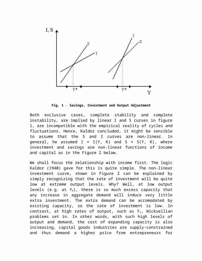
Policy LagsThe use of fiscal policy encounters time lags, or policy lags, between the onset of an economic problem, such as a business-cycle contraction, and the full impact of the policy designed to correct the problem. A business-cycle contraction that hits the economy on January 1st cannot be correct with fiscal policy by January 2nd.

Four types of policy lags are common.

Recognition Lag: This is the time it takes to identify the existence of a problem. It takes time to obtain economic measurements. Once data are obtained, it takes time to analyze and evaluate the data to document the problem.

Decision Lag: This is the time it takes to decide on a suitable course of action, then pass whatever legislation, laws, or administrative rules are needed. For fiscal policy, this requires an act of Congress, signed into law by the President. These decisions could take days, weeks, or even months.

Implementation Lag: This is the time it takes to implement the chosen policy. A spending change requires actions by dozens, hundreds, or even thousands of different government agencies, all of which need to decide on to change their budgets. A tax change requires the distribution of new tax rates and responses by those paying the taxes. The implementation of fiscal policy is also likely to take weeks if not months.

Impact Lag: This lag is the time it takes any change initiated by a government policy to actually impact the producers and consumers in the economy. A key part of the impact lag is the multiplier. A change in government spending or taxes must work its way through the economy, triggering subsequent changes in production and income, which induces changes in consumption, which causes more changes in production and income, which induces further changes in consumption. An impact lag of one to two years is not uncommon.

The goal of fiscal policy is to stabilize the business cycle, to counter contractions and expansions. However, policy lags can cause fiscal policy to destabilize the economy. It can worsen the ups and downs of the business cycle. The impact of expansionary fiscal policy to correct a business-cycle contraction, for example, might occur during the ensuing expansion, which can then over stimulate the economy and cause inflation. Or the impact of contractionary fiscal policy designed to reduce inflation might not occur until the onset of a subsequent contraction. In both cases, the resulting policy is not counter-cyclical, but pro-cyclical.

Automatic StabilizersFiscal policy is intended to be discretionary. That is, policy makers decide to change government spending and taxes in response to business-cycle conditions. However, the economy also has a built-in "fiscal" mechanism that acts to automatically reduce the expansions and contractions of the business cycle.

This mechanism is termed automatic stabilizers. Automatic stabilizers are taxes and transfer payments that depend on the level of aggregate production and income such that

they automatically dampen business-cycle instability without the need for discretionary policy action.

Automatic stabilizers work AUTOMATICALLY. There is no need for Congress or the President to enact legislation, pass bills, or to undertake any other policy action. These stabilizers are built into the structure of the economy. The government sets up the rules and criteria under which taxes and transfer payments work. If people meet the criteria, then they pay the taxes or receive the transfer payments. The amount of each depends on the number of people meeting the criteria, which is dependent on business cycle activity.

Let's take a closer look at each of the two automatic stabilizers -- taxes and transfer payments.

Taxes: Income taxes, especially federal income taxes, largely depend on the level of aggregate production and income in the economy. If production and income rise, then tax collections also rise. Income taxes also tend to be progressive -- the proportion of taxes paid increases with income.

As such, people pay an increasing proportion of income in taxes when the economy expands, leaving proportionally less disposable income available for consumption expenditures and further expansionary stimulation. Moreover, people pay a decreasing proportion of income in taxes when the economy contracts, leaving proportionally more disposable income available for consumption expenditures.

Transfer Payments Transfer payments, including Social Security to the elderly, unemployment compensation to the unemployed, and welfare to the poor, also depend on the level of aggregate production and income. These, however, work opposite to taxes. If aggregate income rises, transfer payments tend to fall as people are less likely to retire, be unemployed, or fall into the ranks of the poor.

As the economy expands, and aggregate income increases, people receive increasingly fewer transfer payments. The consuming public has proportionally less disposable income for consumption expenditures and further expansionary stimulation. As the economy contracts, transfer payments rise; providing lessening the drop in disposable income that would have occurred otherwise.

Automatic stabilizers largely came into existence in response to the Great Depression of the 1930s. In the decade’s preceeding the Great Depression, business cycles tended to be particularly volatile. In the decades following the Great Depression, business cycles were substantially more subdued. Automatic stabilizers are given at least partial credit for the increased stability of recent times.

Politics: Two ViewsPolitics are never far from economics, especially when policies are involved. Such is the case for fiscal policy. In some cases the federal government leans philosophically toward

expansionary fiscal policy and in other cases toward contractionary fiscal policy. The inclination for one type of policy or the other often results from political philosophy--conservative and liberal.

Conservatives tend to favor individual choices over government, producers over consumers, and lower inflation over lower unemployment. Conservatives tend to prefer contractionary fiscal supply. This keeps inflation rates down, even though higher unemployment rates might result.

Liberals tend to favor government restrictions on individual choices, consumers over producers, and lower unemployment over lower inflation. Liberals tend to prefer expansionary fiscal supply. This ensures lower unemployment rates, even though higher inflation rates might result.

The federal government, especially the President, tends to lean more in one political direction or the other. Some Presidents have tended to be more liberal, using fiscal policy to keep unemployment rates low. Others have tended to be more conservative, using fiscal policy to keep inflation rates low. While Presidents, in theory, can be absolutely, positively, completely neutral when it comes to politics, such seldom happens.

Activity 3

1. Discuss various approaches to business cycles. Differentiate between exogenous and endogenous models.

2. What do you understand by Kaldor’s non linear model?

3. write short note on the following:

Fiscal policy Monetary policy Economic policy Credit/Debt cycle

3.7 SUMMARY

This unit is about business cycles and related concepts. After brief introduction various approaches to business cycles are discussed including exogenous vs. endogenous model, Keynesian, Australian school, Credit/Debt cycle, RBC theory etc followed by Schumpeter theory of business cycle. Kaldor’s non linear cycle is discussed as it is distinguishable from most other contemporary treatments since it utilizes non-linear functions. In the Samuelson–Hicks business cycle model, investment is determined by the growth in income, through the principle of acceleration. Next area of concern was implication of policies to control business cycles in which monetary policy is described as controlling of the quantity of money in circulation for the expressed purpose of stabilizing the business cycle and reducing the problems of unemployment and inflation. On the other hand Fiscal policy is based on the presumption that aggregate expenditures, especially business investment, are the primary source of business-cycle instability.

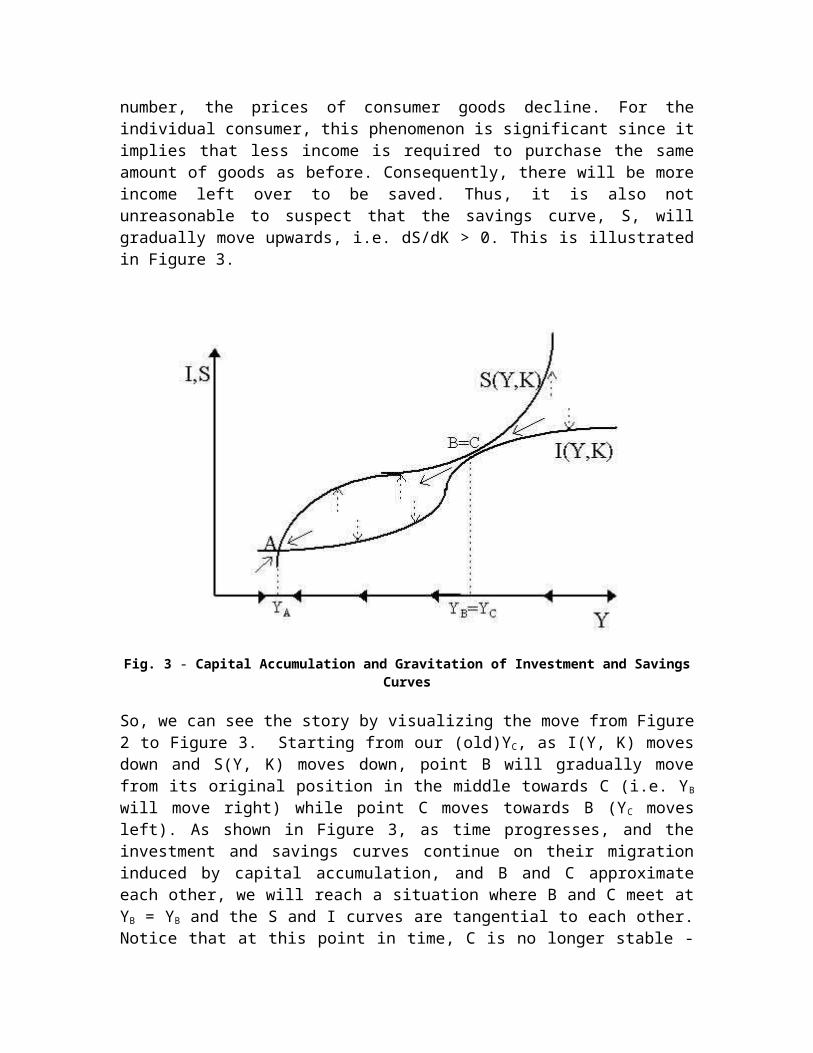
3.8 FURTHER READINGS

M. W. Lee, Economic fluctuations. Homewood, IL, Richard D. Irwin, 1955 Schumpeter, J. A. (1954). History of Economic Analysis. London: George Allen

& Unwin. Kitchin, Joseph (1923). "Cycles and Trends in Economic Factors". Review of

Economics and Statistics F. Burns and W. C. Mitchell, Measuring business cycles, New York, National

Bureau of Economic Research, 1946.