Paper: “Ares I-X Range Safety Simulation Verification and Analysis Independent Validation and Verification” Conference: JANNAF Propulsion Meeting Dates: April 18-22, 2011 The authors from centers other than JSC wrote/contributed to the following pages: Author: A. Scott Craig Pages: 3 - 10 Export control rep: Dave Edwards (EV40), David.l.edwards@nasa.gov Author: Paul Tartabini Pages: 14 - 19 Export control rep: Timothy Robert Woods, timothy.wood@nasa.gov, (757) 864-6933.

https://ntrs.nasa.gov/search.jsp?R=20110008533 2020-07-29T05:59:54+00:00Z

DISTRIBUTION STATEMENT A. Approved for public release; distribution is unlimited.

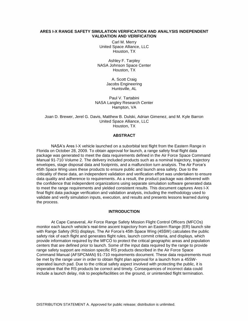
ARES I-X RANGE SAFETY SIMULATION VERIFICATION AND ANALYSIS INDEPENDENT VALIDATION AND VERIFICATION

Carl M. Merry United Space Alliance, LLC

Houston, TX

Ashley F. Tarpley NASA Johnson Space Center

Houston, TX

A. Scott Craig Jacobs Engineering

Huntsville, AL

Paul V. Tartabini NASA Langley Research Center

Hampton, VA

Joan D. Brewer, Jerel G. Davis, Matthew B. Dulski, Adrian Gimenez, and M. Kyle Barron United Space Alliance, LLC

Houston, TX

ABSTRACT

NASA’s Ares I-X vehicle launched on a suborbital test flight from the Eastern Range in Florida on October 28, 2009. To obtain approval for launch, a range safety final flight data package was generated to meet the data requirements defined in the Air Force Space Command Manual 91-710 Volume 2. The delivery included products such as a nominal trajectory, trajectory envelopes, stage disposal data and footprints, and a malfunction turn analysis. The Air Force’s 45th Space Wing uses these products to ensure public and launch area safety. Due to the criticality of these data, an independent validation and verification effort was undertaken to ensure data quality and adherence to requirements. As a result, the product package was delivered with the confidence that independent organizations using separate simulation software generated data to meet the range requirements and yielded consistent results. This document captures Ares I-X final flight data package verification and validation analysis, including the methodology used to validate and verify simulation inputs, execution, and results and presents lessons learned during the process.

INTRODUCTION

At Cape Canaveral, Air Force Range Safety Mission Flight Control Officers (MFCOs) monitor each launch vehicle’s real-time ascent trajectory from an Eastern Range (ER) launch site with Range Safety (RS) displays. The Air Force’s 45th Space Wing (45SW) calculates the public safety risk of each flight and generates flight rules, launch commit criteria, and displays, which provide information required by the MFCO to protect the critical geographic areas and population centers that are defined prior to launch. Some of the input data required by the range to provide range safety support are mission specific RS products described in the Air Force Space Command Manual (AFSPCMAN) 91-710 requirements document. These data requirements must be met by the range user in order to obtain flight plan approval for a launch from a 45SW-operated launch pad. Due to the critical safety aspect involved with protecting the public, it is imperative that the RS products be correct and timely. Consequences of incorrect data could include a launch delay, risk to people/facilities on the ground, or unintended flight termination.

SCOPE OF WORK

The Ares I-X Systems Engineering and Integration (SE&I) Office, located at Langley Research Center (LaRC), worked with teams at Johnson Space Center (JSC), Marshall Space Flight Center (MSFC), Aerospace Corporation in Los Angeles, and the 45SW in the development of the RS products discussed in this paper. The RS products discussed herein were developed using six degree-of-freedom (6DOF) flight simulations and were verified by teams at JSC, MSFC, and Aerospace Corporation. Table 1 lists the prime generation and verification teams for the Ares I-X RS products. In addition to the direct product support teams, the Launch Constellation Range Safety Panel (LCRSP) and its Range Safety Trajectory Working Group (RSTWG) provided direction and review. The 45SW was involved in the RSTWG throughout the generation and IV&V process ensuring the RS product package successfully met all requirements.

Table 1 Ares I-X Roles and Responsibilities

Product Prime IV&V

Nominal Ascent Trajectory LaRC JSC, MSFC

Ascent Flight Envelope Data LaRC MSFC

Malfunction Turn Data LaRC JSC

First Stage Disposal Footprint LaRC Aerospace Corporation

The nominal trajectory is the undispersed, no-fail trajectory predicted to be representative of day-of-launch conditions. The ascent flight envelopes define the trajectory positional downrange and uprange boundaries defined by predicted environmental and systems dispersions. The malfunction turn analysis describes the off-nominal trajectories that may result from a single system failure. The first stage (FS) disposal impact footprint encompasses impact locations resulting from FS reentries with system and environmental dispersions. Please refer to the papers listed in the references section for detail on each of these products.

RESULTS AND DISCUSSION

The Ares I-X project employed an independent verification and validation (IV&V) process for the Final Flight Data Package (FFDP) to ensure the proper products were developed and the products delivered were accurate to the greatest extent possible and free of errors. This paper describes the IV&V efforts undertaken for the following RS products: nominal ascent trajectory, ascent flight envelopes, malfunction turn data and analysis, and stage disposal footprint. The Ares I-X RS product analysis, strengthened by the rigor of the IV&V effort, produced vehicle trajectory data that was on-time and error free, contributing to the successful launch of Ares I-X.

VALIDATION

Validation of the FFDP data product was achieved through the work of the RSTWG. The RSTWG consisted of personnel from Ares I-X System Engineering and Integration (SE&I) trajectory team (at LaRC), Johnson Space Center’s range safety and probabilistic risk assessment teams, United Space Alliance (USA) contractors at JSC, and Willbrook and Jacobs Engineering contractors at Marshall Space Flight Center. The Ares I-X SE&I trajectory team worked in conjunction with the other RSTWG members and the 45SW to develop the FFDP data product requirements using the AFSPCMAN 91-710 Volume 2, that was tailored to the Ares I-X test flight. Regular RSTWG meetings were held with the 45SW in attendance to provide a forum for identifying all requirements applicable to the flight test vehicle (FTV) and for developing appropriate methods to generate and verify those data products. The 45SW’s participation in the meetings provided guidance in properly understanding and interpreting the requirements and provided assurance that the method used to generate the products was acceptable. The JSC RSTWG team members have experience developing Space Shuttle Range Safety products. Their experience was combined with SE&I trajectory team’s knowledge of the FTV to develop the best

method for producing Ares I-X specific data products that incorporate lessons learned throughout the Shuttle program.

VERIFICATION

Verification of the FFDP data product’s accuracy and correctness was achieved through agreement between redundant FFDP data products generated by analysis teams at multiple NASA Centers using different simulation software. Each trajectory data product was developed by two separate analysis teams using simulation software specific to each team. Each analysis team implemented Ares I-X FTV specific models into their simulation software and performed their analyses as agreed upon in the RSTWG forum. The verification process consisted of two phases, simulation verification and results verification. Simulation verification was the process of verifying that each team’s vehicle, mission, and environmental inputs are obtained from the same source and that they are implemented correctly in each simulation. This was referred to as quality assurance (QA) verification in the RSTWG forum. Results verification was the process of verifying that all simulation runs required to generate the FFDP data products have been completed and that the data products are error free. Both QA and results verification were achieved through comparison of simulation output between the analysis teams. The verification approach assumed that if a model implementation error occurs or if an error occurs in the results generation, it does not manifest itself in both simulations in the same manner and will be identifiable through comparison of simulation results.

SIMULATION COMPARISON OVERVIEW

Each team worked with an Ares I-X tailored version of a 6DOF simulation. These will be referred to by the common name of the respective simulation throughout this paper: LaRC used Program to Optimize Simulated Trajectories II (POST2), JSC used Advanced NASA Technology Architecture for Exploration Studies (ANTARES), MSFC used Marshall Aerospace Vehicle Representation In C (MAVERIC).Two simulations involved in the RS process, but not directly involved in this Range Safety specific comparison were LaSRS and PROCONSUL. LaSRS was the simulation used in development of the Ares I-X Guidance and Control flight software. PROCONSUL was the simulation used by the Aerospace Corporation to verify the disposal footprints.

Extensive simulation verification was performed prior to the start of the product generation. This activity served to ensure that each vehicle and environmental model was implemented properly, and that the methodology and implementation of the system dispersions, environmental dispersions, and failure modes were consistent. The verification process did not address the accuracy of input models. It was assumed that the developers of the individual models were responsible for the validation and accuracy of their model.

As updates were provided by the project, referenced data was incorporated into the simulation. Table data, such as aerodynamic and mass properties, were transferred into their corresponding formats and coordinate frames. Verification of the implementation was conducted by running a test matrix, defined by the RSTWG, and comparing new models with prior released models. Any discrepancies were noted and further investigated to determine if there were issues with a specific simulation or if it occurred across all simulations. As each model was updated, its original source and date were noted and tracked in a common configuration management (CM) spreadsheet. This CM spreadsheet served the purpose of a math model database. It not only tracked the latest models, but also the implementation in the simulations. This was useful when it became necessary to make sure the latest updates were in a specific simulation; the spreadsheet was consulted and one could trace the project approved data to the file in which it was implemented.

Both quantitative and qualitative comparisons were performed. Quantitative (required) metric violations were investigated to identify and correct the root cause. Qualitative (desired) metrics exceeded were evaluated within the allowable timeframe in an effort to resolve the

difference. Raw comparison data took two forms: a 152 parameter set defined by the Ares I-X Guidance and Control (G&C) simulation community and an RS specific set covering the delivery data as well as malfunction related parameters.

Significant effort went into automating the execution and comparison of the trajectories. This effort was well placed. Every time a new model was delivered, a malfunction implementation was modified or the launch date slipped, the compared trajectories were regenerated, verified, and compared. This was determined to be the only way to maintain adequate confidence that mistakes weren’t being introduced during the occasionally rapid update cycle.

NOMINAL TRAJECTORY COMPARISON METHODOLOGY

The nominal ascent trajectory is the baseline for all RS data products delivered to the Range. If there was any error in the trajectory simulation, it would manifest itself throughout the RS products. Several vehicle specific models were required to complete the nominal simulation:

• Guidance and control flight software

• Aerodynamics

• Mass properties

• Propulsion characteristics: ATK Solid Rocket Booster, reaction control thrusters

While the IV&V activity did not verify that each of these models accurately reflected the vehicle configuration, the independent nature of implementing these models provided an indication that the models were implemented correctly. This assumes that because the same model is being implemented in two different simulations, the implementations would vary and therefore a common error occurring is unlikely.

Tests of individual models (unit tests) were not compared between organizations; only integrated simulation results were compared. There is risk associated with this approach of making it more difficult to determine the source of a particular discrepancy. For example, an error in the gimbal location of the main engine will result in a mismatch between commanded deflections and moments induced on the vehicle. The control system will respond to the corresponding rates with gimbal corrections. The analyst troubleshooting this problem may have difficulty determining if the control system implementation is causing or responding to the issue.

TOLERANCE DEVELOPMENT

Exact matches between simulations were not required in order to verify accuracy. It was understood that different methodologies produce different results, but both can be representative of the truth. Quantifying the magnitude of an acceptable deviation between simulations, especially for the first flight of a new vehicle, can be challenging.

Some tolerances were derived from simulation comparison tolerances used by the Space Shuttle Day-of-Launch I-Load Update (DOLILU) process, however these tolerances have been honed over years of operations where differences can be eliminated by repeated analyses. In addition, some of the tolerances are particular to the nature of the trajectory designed for the Space Shuttle.

Additional tolerances were derived from an interpretation of how the range safety products are processed. The impact point of the vehicle is a key parameter of the trajectory data used by the 45SW. Thus tolerances were derived based on the effects of differences in certain state parameters on the corresponding differences in downrange and cross range impact position. In effect, the partial derivatives of position and velocity components with respect to cross range and down range were computed by perturbing individual state parameters. These partials were formally computed at LaRC and confirmed with a similar analysis conducted by the JSC IV&V team.

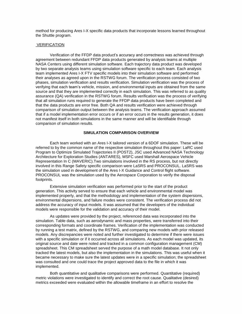
NOMINAL TRAJECTORY COMPARISON RESULTS

Figure 1 contains a summary of the comparisons between POST2 and the verification simulations for the no wind and mean July winds case. The zero wind trajectory was used to isolate wind related effects and eliminate wind as a cause of control software related issues. All results were within the tolerances except for the pitch and/or yaw attitudes at separation. These differences were deemed acceptable since they were minor violations and they fell under the qualitative category. The critical parameters contained in the quantitative comparisons were all within the tolerances.

Four other simulations varying only the wind were also performed using worst case directional winds. Worst case winds were not measured winds but instead were worst case winds from a RS perspective in that they assumed the maximum reasonable wind at all altitudes in the four cardinal directions: north, east, south, and west. A worst case wind in a single direction maximizes the effect of wind on the impact footprint. These wind cases were also compared and compare in a similar fashion to the no wind and mean wind cases. Only the pitch and/or yaw attitudes at separation were outside the tolerance; all other comparisons were within the tolerances.

Figure 1 Notional Quantitative Simulation Comparison Data

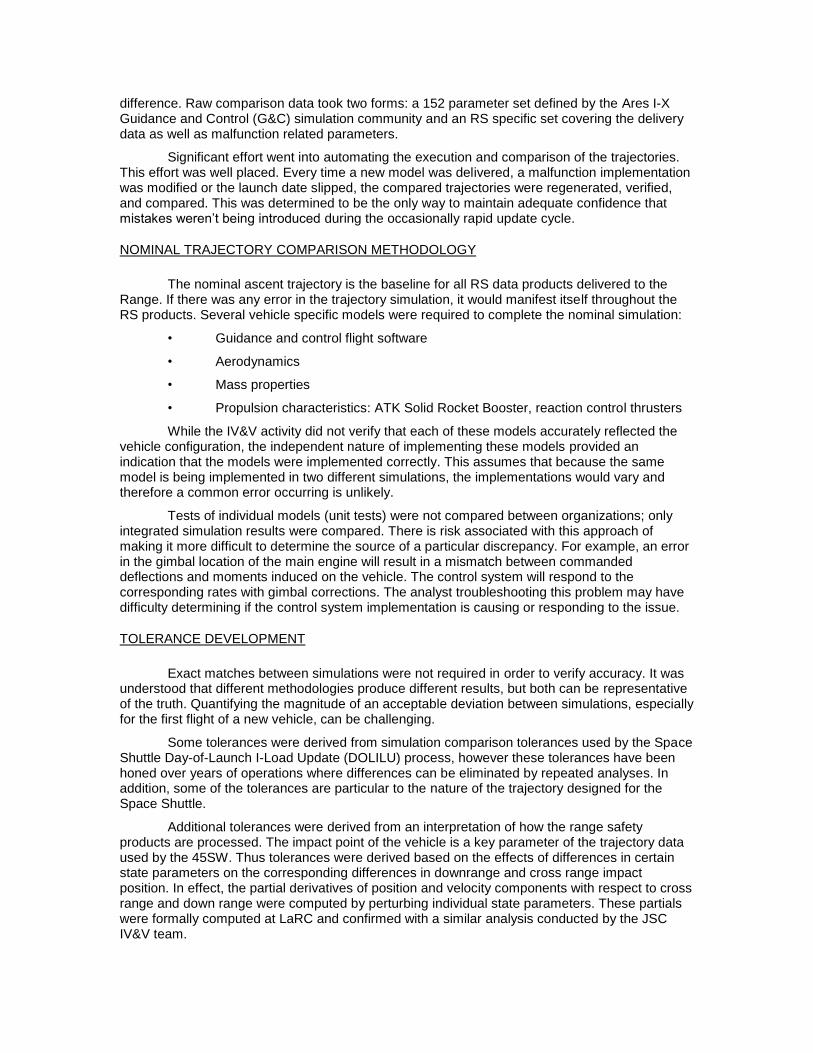
The match criteria were also compared as time history plots. Time history plots were

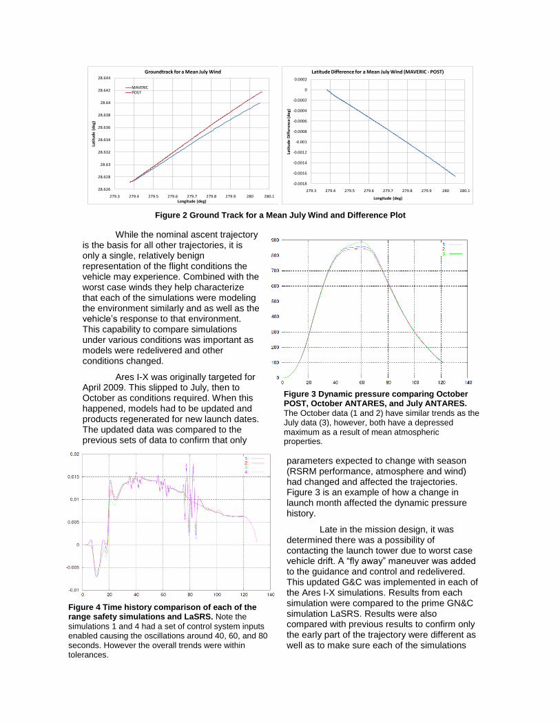
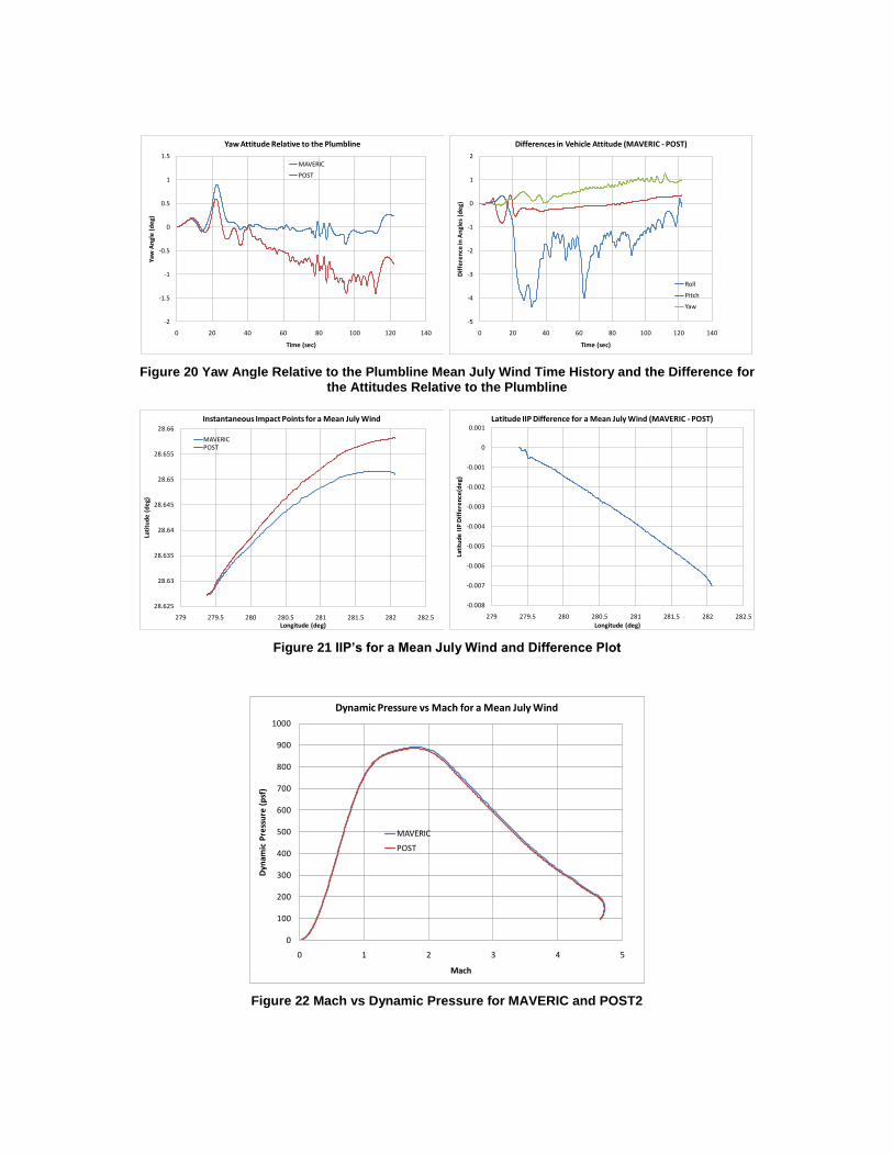
qualitative criteria. Each parameter of the comparison data was co-plotted in this manner to confirm that the trajectories were similar from solid rocket booster (SRB) ignition through commanded staging. Figure 2 is an example groundtrack plot for a mean July wind. Note that the latitude scale (and thus trajectory difference) is exaggerated due to the nature of the trajectory (due East). Additional time history plots can be found in Appendix A.

28.626

28.628

28.63

28.632

28.634

28.636

28.638

28.64

28.642

28.644

279.3 279.4 279.5 279.6 279.7 279.8 279.9 280 280.1

Lati

tud

e (

de

g)

Longitude (deg)

Groundtrack for a Mean July Wind

MAVERICPOST

-0.0018

-0.0016

-0.0014

-0.0012

-0.001

-0.0008

-0.0006

-0.0004

-0.0002

0

0.0002

279.3 279.4 279.5 279.6 279.7 279.8 279.9 280 280.1

Lati

tud

e D

iffe

ren

ce (d

eg)

Longitude (deg)

Latitude Difference for a Mean July Wind (MAVERIC - POST)

Figure 2 Ground Track for a Mean July Wind and Difference Plot

While the nominal ascent trajectory is the basis for all other trajectories, it is only a single, relatively benign representation of the flight conditions the vehicle may experience. Combined with the worst case winds they help characterize that each of the simulations were modeling the environment similarly and as well as the vehicle’s response to that environment. This capability to compare simulations under various conditions was important as models were redelivered and other conditions changed.

Ares I-X was originally targeted for April 2009. This slipped to July, then to October as conditions required. When this happened, models had to be updated and products regenerated for new launch dates. The updated data was compared to the previous sets of data to confirm that only

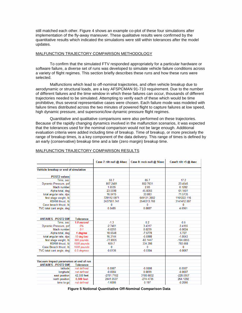
parameters expected to change with season (RSRM performance, atmosphere and wind) had changed and affected the trajectories. Figure 3 is an example of how a change in launch month affected the dynamic pressure history.

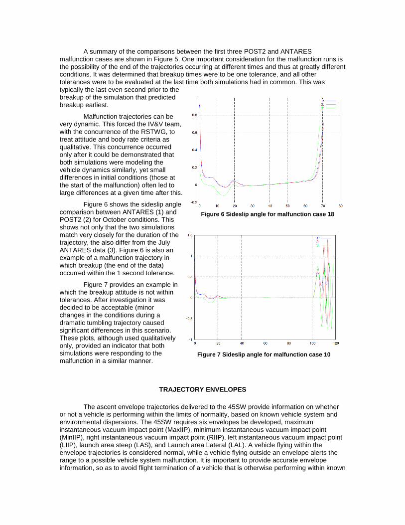
Late in the mission design, it was determined there was a possibility of contacting the launch tower due to worst case vehicle drift. A “fly away” maneuver was added to the guidance and control and redelivered. This updated G&C was implemented in each of the Ares I-X simulations. Results from each simulation were compared to the prime GN&C simulation LaSRS. Results were also compared with previous results to confirm only the early part of the trajectory were different as well as to make sure each of the simulations

Figure 4 Time history comparison of each of the range safety simulations and LaSRS. Note the

simulations 1 and 4 had a set of control system inputs enabled causing the oscillations around 40, 60, and 80 seconds. However the overall trends were within tolerances.

Figure 3 Dynamic pressure comparing October POST, October ANTARES, and July ANTARES.

The October data (1 and 2) have similar trends as the July data (3), however, both have a depressed maximum as a result of mean atmospheric properties.

still matched each other. Figure 4 shows an example co-plot of these four simulations after implementation of the fly-away maneuver. These qualitative results were confirmed by the quantitative results which indicated the simulations were still within tolerances after the model updates.

MALFUNCTION TRAJECTORY COMPARISON METHODOLOGY

To confirm that the simulated FTV responded appropriately for a particular hardware or software failure, a diverse set of runs was developed to simulate vehicle failure conditions across a variety of flight regimes. This section briefly describes these runs and how these runs were selected.

Malfunctions which lead to off-nominal trajectories, and often vehicle breakup due to aerodynamic or structural loads, are a key AFSPCMAN 91-710 requirement. Due to the number of different failures and the time window in which these failures can occur, thousands of different trajectories needed to be simulated. Attempting to verify each of these which would be time prohibitive, thus several representative cases were chosen. Each failure mode was modeled with failure times distributed across the two minutes of powered flight to capture failures at low speed, high dynamic pressure, and supersonic/low dynamic pressure flight regimes.

Quantitative and qualitative comparisons were also performed on these trajectories. Because of the rapidly changing dynamics involved in the malfunction scenarios, it was expected that the tolerances used for the nominal comparison would not be large enough. Additional evaluation criteria were added including time of breakup. Time of breakup, or more precisely the range of breakup times, is a key component of the data delivery. This range of times is defined by an early (conservative) breakup time and a late (zero margin) breakup time.

MALFUNCTION TRAJECTORY COMPARISON RESULTS

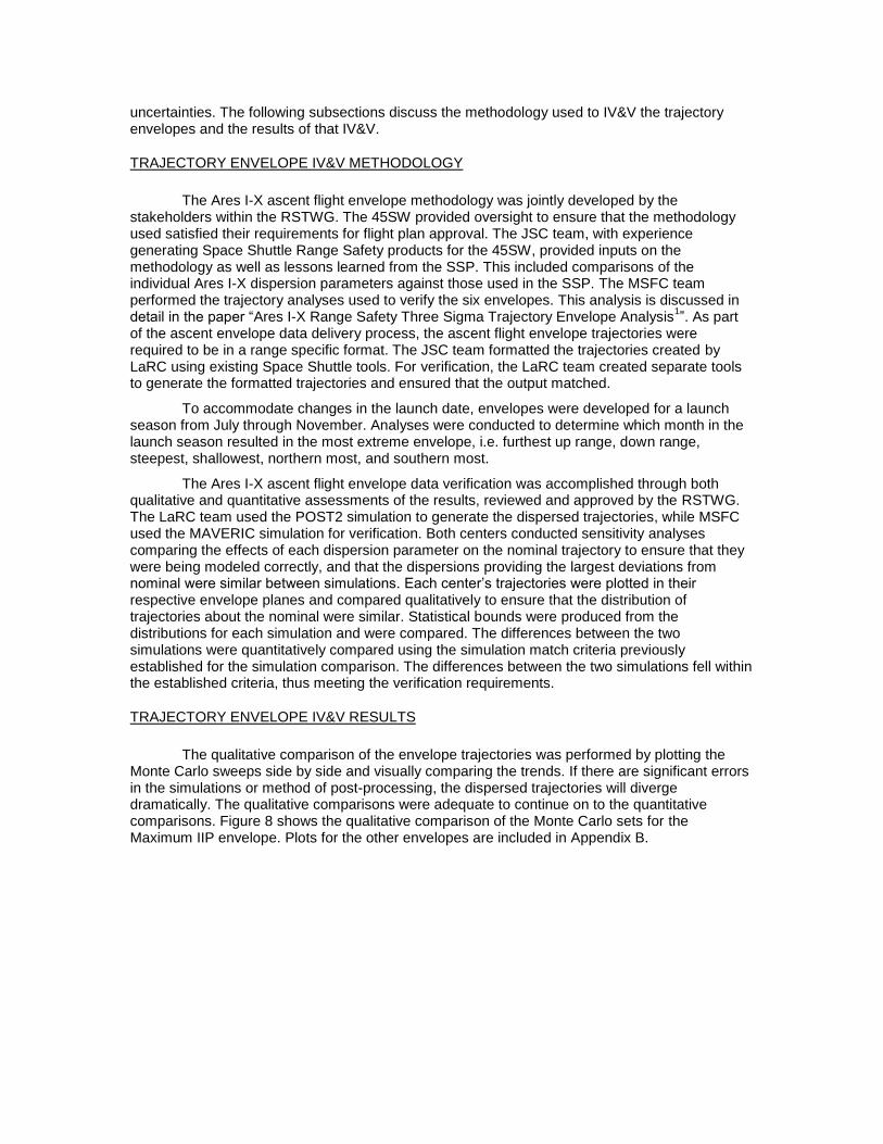
Figure 5 Notional Quantitative Off-Nominal Comparison Data

A summary of the comparisons between the first three POST2 and ANTARES malfunction cases are shown in Figure 5. One important consideration for the malfunction runs is the possibility of the end of the trajectories occurring at different times and thus at greatly different conditions. It was determined that breakup times were to be one tolerance, and all other tolerances were to be evaluated at the last time both simulations had in common. This was typically the last even second prior to the breakup of the simulation that predicted breakup earliest.

Malfunction trajectories can be very dynamic. This forced the IV&V team, with the concurrence of the RSTWG, to treat attitude and body rate criteria as qualitative. This concurrence occurred only after it could be demonstrated that both simulations were modeling the vehicle dynamics similarly, yet small differences in initial conditions (those at the start of the malfunction) often led to large differences at a given time after this.

Figure 6 shows the sideslip angle comparison between ANTARES (1) and POST2 (2) for October conditions. This shows not only that the two simulations match very closely for the duration of the trajectory, the also differ from the July ANTARES data (3). Figure 6 is also an example of a malfunction trajectory in which breakup (the end of the data) occurred within the 1 second tolerance.

Figure 7 provides an example in which the breakup attitude is not within tolerances. After investigation it was decided to be acceptable (minor changes in the conditions during a dramatic tumbling trajectory caused significant differences in this scenario. These plots, although used qualitatively only, provided an indicator that both simulations were responding to the malfunction in a similar manner.

TRAJECTORY ENVELOPES

The ascent envelope trajectories delivered to the 45SW provide information on whether or not a vehicle is performing within the limits of normality, based on known vehicle system and environmental dispersions. The 45SW requires six envelopes be developed, maximum instantaneous vacuum impact point (MaxIIP), minimum instantaneous vacuum impact point (MinIIP), right instantaneous vacuum impact point (RIIP), left instantaneous vacuum impact point (LIIP), launch area steep (LAS), and Launch area Lateral (LAL). A vehicle flying within the envelope trajectories is considered normal, while a vehicle flying outside an envelope alerts the range to a possible vehicle system malfunction. It is important to provide accurate envelope information, so as to avoid flight termination of a vehicle that is otherwise performing within known

Figure 7 Sideslip angle for malfunction case 10

Figure 6 Sideslip angle for malfunction case 18

uncertainties. The following subsections discuss the methodology used to IV&V the trajectory envelopes and the results of that IV&V.

TRAJECTORY ENVELOPE IV&V METHODOLOGY

The Ares I-X ascent flight envelope methodology was jointly developed by the stakeholders within the RSTWG. The 45SW provided oversight to ensure that the methodology used satisfied their requirements for flight plan approval. The JSC team, with experience generating Space Shuttle Range Safety products for the 45SW, provided inputs on the methodology as well as lessons learned from the SSP. This included comparisons of the individual Ares I-X dispersion parameters against those used in the SSP. The MSFC team performed the trajectory analyses used to verify the six envelopes. This analysis is discussed in detail in the paper “Ares I-X Range Safety Three Sigma Trajectory Envelope Analysis

1”. As part

of the ascent envelope data delivery process, the ascent flight envelope trajectories were required to be in a range specific format. The JSC team formatted the trajectories created by LaRC using existing Space Shuttle tools. For verification, the LaRC team created separate tools to generate the formatted trajectories and ensured that the output matched.

To accommodate changes in the launch date, envelopes were developed for a launch season from July through November. Analyses were conducted to determine which month in the launch season resulted in the most extreme envelope, i.e. furthest up range, down range, steepest, shallowest, northern most, and southern most.

The Ares I-X ascent flight envelope data verification was accomplished through both qualitative and quantitative assessments of the results, reviewed and approved by the RSTWG. The LaRC team used the POST2 simulation to generate the dispersed trajectories, while MSFC used the MAVERIC simulation for verification. Both centers conducted sensitivity analyses comparing the effects of each dispersion parameter on the nominal trajectory to ensure that they were being modeled correctly, and that the dispersions providing the largest deviations from nominal were similar between simulations. Each center’s trajectories were plotted in their respective envelope planes and compared qualitatively to ensure that the distribution of trajectories about the nominal were similar. Statistical bounds were produced from the distributions for each simulation and were compared. The differences between the two simulations were quantitatively compared using the simulation match criteria previously established for the simulation comparison. The differences between the two simulations fell within the established criteria, thus meeting the verification requirements.

TRAJECTORY ENVELOPE IV&V RESULTS

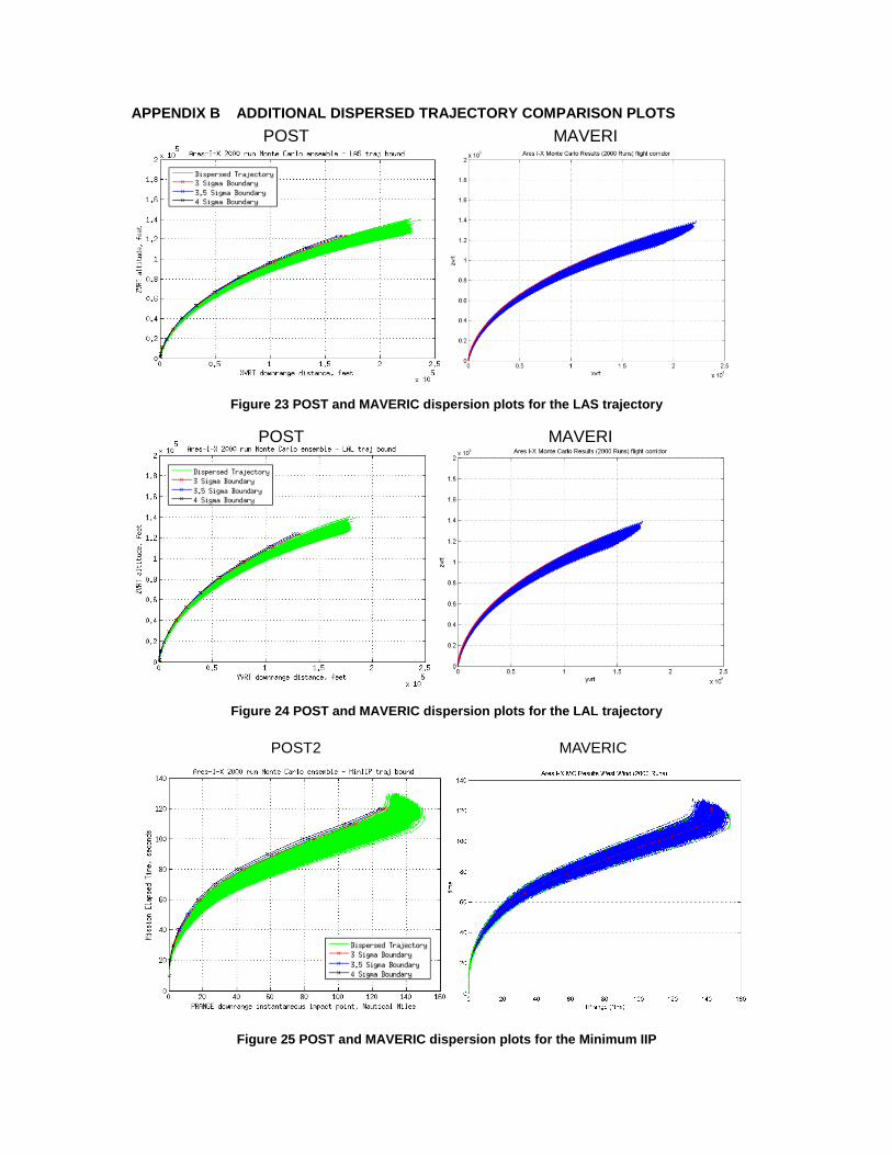
The qualitative comparison of the envelope trajectories was performed by plotting the Monte Carlo sweeps side by side and visually comparing the trends. If there are significant errors in the simulations or method of post-processing, the dispersed trajectories will diverge dramatically. The qualitative comparisons were adequate to continue on to the quantitative comparisons. Figure 8 shows the qualitative comparison of the Monte Carlo sets for the Maximum IIP envelope. Plots for the other envelopes are included in Appendix B.

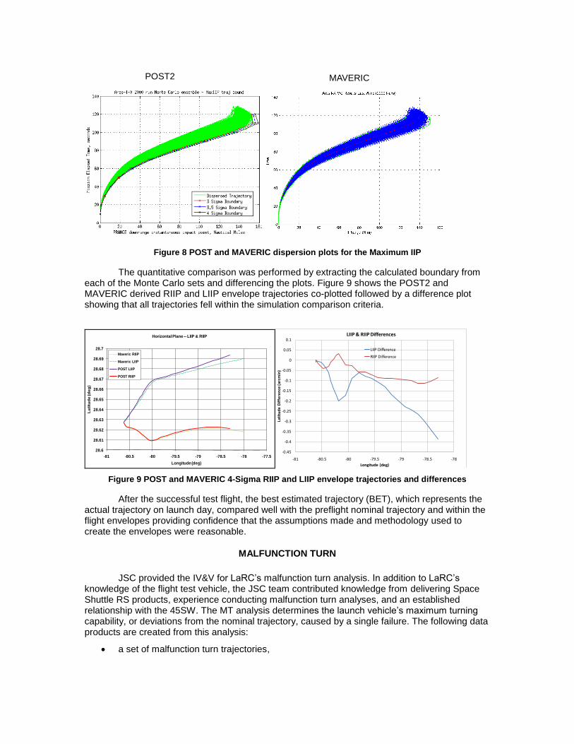
POST2 MAVERIC

Figure 8 POST and MAVERIC dispersion plots for the Maximum IIP

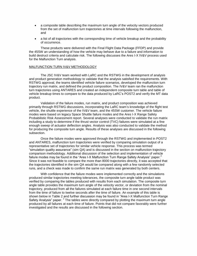
The quantitative comparison was performed by extracting the calculated boundary from each of the Monte Carlo sets and differencing the plots. Figure 9 shows the POST2 and MAVERIC derived RIIP and LIIP envelope trajectories co-plotted followed by a difference plot showing that all trajectories fell within the simulation comparison criteria.

28.6

28.61

28.62

28.63

28.64

28.65

28.66

28.67

28.68

28.69

28.7

-81 -80.5 -80 -79.5 -79 -78.5 -78 -77.5

La

titu

de

(d

eg

)

Longitude (deg)

Horizontal Plane -- LIIP & RIIP

Maveric RIIP

Maveric LIIP

POST LIIP

POST RIIP

-0.45

-0.4

-0.35

-0.3

-0.25

-0.2

-0.15

-0.1

-0.05

0

0.05

0.1

-81 -80.5 -80 -79.5 -79 -78.5 -78

Lati

tud

e D

iffe

ren

ce (a

rcm

in)

Longitude (deg)

LIIP & RIIP Differences

LIIP Difference

RIIP Difference

Figure 9 POST and MAVERIC 4-Sigma RIIP and LIIP envelope trajectories and differences

After the successful test flight, the best estimated trajectory (BET), which represents the actual trajectory on launch day, compared well with the preflight nominal trajectory and within the flight envelopes providing confidence that the assumptions made and methodology used to create the envelopes were reasonable.

MALFUNCTION TURN

JSC provided the IV&V for LaRC’s malfunction turn analysis. In addition to LaRC’s knowledge of the flight test vehicle, the JSC team contributed knowledge from delivering Space Shuttle RS products, experience conducting malfunction turn analyses, and an established relationship with the 45SW. The MT analysis determines the launch vehicle’s maximum turning capability, or deviations from the nominal trajectory, caused by a single failure. The following data products are created from this analysis:

a set of malfunction turn trajectories,

a composite table describing the maximum turn angle of the velocity vectors produced from the set of malfunction turn trajectories at time intervals following the malfunction, and

a list of all trajectories with the corresponding time of vehicle breakup and the probability of occurrence.

These products were delivered with the Final Flight Data Package (FFDP) and provide the 45SW an understanding of how the vehicle may behave due to a failure and information to build destruct criteria and calculate risk. The following discusses the Ares I-X IV&V process used for the Malfunction Turn analysis.

MALFUNCTION TURN IV&V METHODOLOGY

The JSC IV&V team worked with LaRC and the RSTWG in the development of analysis and product generation methodology to validate that the analysis satisfied the requirements. With RSTWG approval, the teams identified vehicle failure scenarios, developed the malfunction turn trajectory run matrix, and defined the product composition. The IV&V team ran the malfunction turn trajectories using ANTARES and created an independent composite turn table and table of vehicle breakup times to compare to the data produced by LaRC’s POST2 and verify the MT data product.

Validation of the failure modes, run matrix, and product composition was achieved primarily through RSTWG discussions, incorporating the LaRC team’s knowledge of the flight test vehicle, the shuttle experience of the IV&V team, and the 45SW customer. The vehicle failure modes were based on legacy Space Shuttle failure modes and the Ares I-X Range Safety Probabilistic Risk Assessment report. Several analyses were conducted to validate the run matrix including a study to determine if the thrust vector control (TVC) failures were simulated at a fine enough sweep of actuator deflection angles. Analysis was also conducted to validate the method for producing the composite turn angle. Results of these analyses are discussed in the following subsection.

Once the failure modes were approved through the RSTWG and implemented in POST2 and ANTARES, malfunction turn trajectories were verified by comparing simulation output of a representative set of trajectories for similar vehicle response. This process was termed “simulation quality assurance” (sim QA) and is discussed in the section on malfunction trajectory comparison methodology. Additional discussion of the selection and implementation of vehicle failure modes may be found in the “Ares I-X Malfunction Turn Range Safety Analysis” paper.

2

Since it was not feasible to compare the more than 8000 trajectories directly, it was accepted that the trajectories identified in the sim QA would be compared along with a few randomly selected runs, and a check was made to confirm the same run matrix was generated by both centers.

With confidence that the failure modes were implemented correctly and the simulations produced similar trajectories meeting tolerances, the composite turn angle table product was verified by comparing the tables produced with results from each simulation. The composite turn angle table provides the maximum turn angle of the velocity vector, or deviation from the nominal trajectory, produced from all the failures simulated at each failure time in one second intervals from the time of failure to twelve seconds after the time of failure. An example of this table is shown below in Table 2 and further discussion may be found in “Ares I-X Malfunction Turn Range Safety Analysis” paper.

2 The tables were directly compared by plotting the maximum turn angle

produced by all failures at each time of failure. Points that did not compare favorably were further investigated and the results are discussed in the following section.

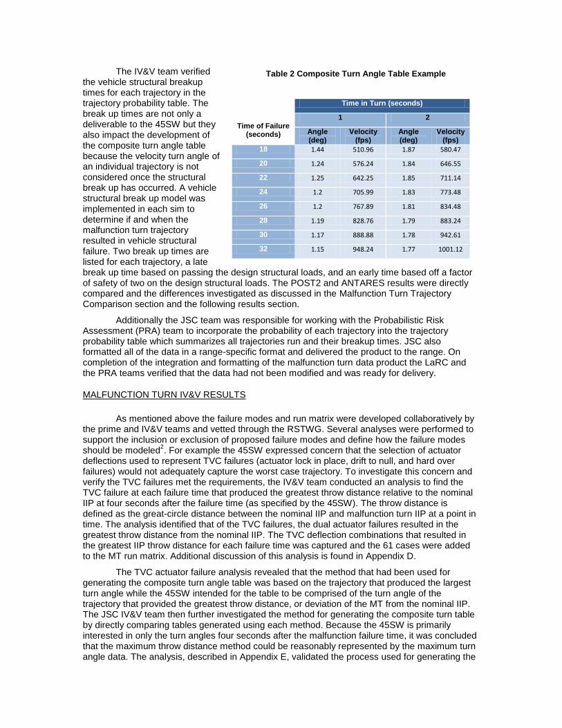
The IV&V team verified the vehicle structural breakup times for each trajectory in the trajectory probability table. The break up times are not only a deliverable to the 45SW but they also impact the development of the composite turn angle table because the velocity turn angle of an individual trajectory is not considered once the structural break up has occurred. A vehicle structural break up model was implemented in each sim to determine if and when the malfunction turn trajectory resulted in vehicle structural failure. Two break up times are listed for each trajectory, a late break up time based on passing the design structural loads, and an early time based off a factor of safety of two on the design structural loads. The POST2 and ANTARES results were directly compared and the differences investigated as discussed in the Malfunction Turn Trajectory Comparison section and the following results section.

Additionally the JSC team was responsible for working with the Probabilistic Risk Assessment (PRA) team to incorporate the probability of each trajectory into the trajectory probability table which summarizes all trajectories run and their breakup times. JSC also formatted all of the data in a range-specific format and delivered the product to the range. On completion of the integration and formatting of the malfunction turn data product the LaRC and the PRA teams verified that the data had not been modified and was ready for delivery.

MALFUNCTION TURN IV&V RESULTS

As mentioned above the failure modes and run matrix were developed collaboratively by the prime and IV&V teams and vetted through the RSTWG. Several analyses were performed to support the inclusion or exclusion of proposed failure modes and define how the failure modes should be modeled

2. For example the 45SW expressed concern that the selection of actuator

deflections used to represent TVC failures (actuator lock in place, drift to null, and hard over failures) would not adequately capture the worst case trajectory. To investigate this concern and verify the TVC failures met the requirements, the IV&V team conducted an analysis to find the TVC failure at each failure time that produced the greatest throw distance relative to the nominal IIP at four seconds after the failure time (as specified by the 45SW). The throw distance is defined as the great-circle distance between the nominal IIP and malfunction turn IIP at a point in time. The analysis identified that of the TVC failures, the dual actuator failures resulted in the greatest throw distance from the nominal IIP. The TVC deflection combinations that resulted in the greatest IIP throw distance for each failure time was captured and the 61 cases were added to the MT run matrix. Additional discussion of this analysis is found in Appendix D.

The TVC actuator failure analysis revealed that the method that had been used for generating the composite turn angle table was based on the trajectory that produced the largest turn angle while the 45SW intended for the table to be comprised of the turn angle of the trajectory that provided the greatest throw distance, or deviation of the MT from the nominal IIP. The JSC IV&V team then further investigated the method for generating the composite turn table by directly comparing tables generated using each method. Because the 45SW is primarily interested in only the turn angles four seconds after the malfunction failure time, it was concluded that the maximum throw distance method could be reasonably represented by the maximum turn angle data. The analysis, described in Appendix E, validated the process used for generating the

Table 2 Composite Turn Angle Table Example

Time in Turn (seconds)

Time of Failure

(seconds)

1 2

Angle (deg)

Velocity (fps)

Angle (deg)

Velocity (fps)

18 1.44 510.96 1.87 580.47

20 1.24 576.24 1.84 646.55

22 1.25 642.25 1.85 711.14

24 1.2 705.99 1.83 773.48

26 1.2 767.89 1.81 834.48

28 1.19 828.76 1.79 883.24

30 1.17 888.88 1.78 942.61

32 1.15 948.24 1.77 1001.12

composite turn angle table was reasonable for this vehicle, but future vehicle malfunction turn analyses would be required to build the table with angles from the trajectories with the greatest throw distance.

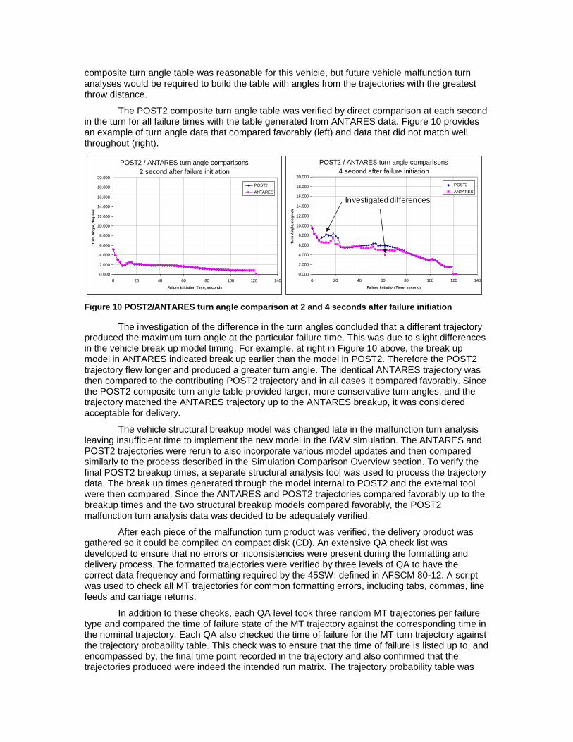
The POST2 composite turn angle table was verified by direct comparison at each second in the turn for all failure times with the table generated from ANTARES data. Figure 10 provides an example of turn angle data that compared favorably (left) and data that did not match well throughout (right).

POST2 / ANTARES turn angle comparisons

2 second after failure initiation

0.000

2.000

4.000

6.000

8.000

10.000

12.000

14.000

16.000

18.000

20.000

0 20 40 60 80 100 120 140

Failure Initiation Time, seconds

Tu

rn A

ng

le, d

eg

rees

POST2

ANTARES

POST2 / ANTARES turn angle comparisons

4 second after failure initiation

0.000

2.000

4.000

6.000

8.000

10.000

12.000

14.000

16.000

18.000

20.000

0 20 40 60 80 100 120 140

Failure Initiation Time, seconds

Tu

rn A

ng

le, d

eg

rees

POST2

ANTARES

Investigated differences

Figure 10 POST2/ANTARES turn angle comparison at 2 and 4 seconds after failure initiation

The investigation of the difference in the turn angles concluded that a different trajectory produced the maximum turn angle at the particular failure time. This was due to slight differences in the vehicle break up model timing. For example, at right in Figure 10 above, the break up model in ANTARES indicated break up earlier than the model in POST2. Therefore the POST2 trajectory flew longer and produced a greater turn angle. The identical ANTARES trajectory was then compared to the contributing POST2 trajectory and in all cases it compared favorably. Since the POST2 composite turn angle table provided larger, more conservative turn angles, and the trajectory matched the ANTARES trajectory up to the ANTARES breakup, it was considered acceptable for delivery.

The vehicle structural breakup model was changed late in the malfunction turn analysis leaving insufficient time to implement the new model in the IV&V simulation. The ANTARES and POST2 trajectories were rerun to also incorporate various model updates and then compared similarly to the process described in the Simulation Comparison Overview section. To verify the final POST2 breakup times, a separate structural analysis tool was used to process the trajectory data. The break up times generated through the model internal to POST2 and the external tool were then compared. Since the ANTARES and POST2 trajectories compared favorably up to the breakup times and the two structural breakup models compared favorably, the POST2 malfunction turn analysis data was decided to be adequately verified.

After each piece of the malfunction turn product was verified, the delivery product was gathered so it could be compiled on compact disk (CD). An extensive QA check list was developed to ensure that no errors or inconsistencies were present during the formatting and delivery process. The formatted trajectories were verified by three levels of QA to have the correct data frequency and formatting required by the 45SW; defined in AFSCM 80-12. A script was used to check all MT trajectories for common formatting errors, including tabs, commas, line feeds and carriage returns.

In addition to these checks, each QA level took three random MT trajectories per failure type and compared the time of failure state of the MT trajectory against the corresponding time in the nominal trajectory. Each QA also checked the time of failure for the MT turn trajectory against the trajectory probability table. This check was to ensure that the time of failure is listed up to, and encompassed by, the final time point recorded in the trajectory and also confirmed that the trajectories produced were indeed the intended run matrix. The trajectory probability table was

also checked numerically. Each QA level added the probabilities for each failure type and checked against the Probabilistic Risk Assessment (PRA) document for consistency.

A numerical difference was also done between the final delivery CD and that contained on the drive. This check verified that all trajectories had a relative tolerance of 1.0E-5 and an absolute tolerance of 1.0E-8 to both the formatted and original non-formatted trajectories provided by LaRC.

DISPOSAL

The disposal footprints delivered to the 45SW provide information on where the spent First Stage (FS) and Upper Stage Simulator (USS) were predicted to land in the water at the end of the test flight. These footprints were delivered as 3-sigma impact ellipses that represented the range of expected landing locations (latitude/longitude coordinates) of each stage at the time of water impact. These impact ellipses were used by the 45SW to establish keepout zones for ship and aircraft traffic and to determine ship placement for first stage tracking and recovery vessels. To compute these ellipses a multi-body reentry trajectory simulation was developed that modeled the descent of both stages from the time of separation until water impact. Both stages’ descents were uncontrolled. The 3-sigma ellipses were determined from 2,000 Monte Carlo runs that modeled off-nominal dispersions in winds, atmosphere, mass properties, vehicle propulsion and aerodynamics. Dispersions on initial state (position, velocity, attitude and attitude rate) were also considered and were obtained from the Ares I-X trajectory envelope Monte Carlo analysis discussed in the previous sections. The following subsections describe the method in which these disposal footprints were verified and present some of the key verification results

DISPOSAL IV&V METHODOLOGY

The disposal footprints delivered to the 45SW were computed by LaRC using POST2. A separate multi-body reentry simulation was developed for verification by the Aerospace Corporation using PROCONSUL, an Aerospace-developed simulation tool which wraps static vehicle data (i.e. mass properties information, propulsion tables, aerodynamic coefficient tables, etc) and event sequencing around FORTRAN 95 dynamics code. Integration of dynamic states is performed within PROCONSUL using a fourth-order Runge-Kutta methodology with variable step size.

4

A two-step verification process was employed to ensure that simulation models were implemented properly and that the corresponding simulation results were accurate. The first step was a QA check that focused on verifying each individual simulation model. To perform this check each simulation model was implemented independently in both POST2 and PROCONSUL and a nominal trajectory was run without any dispersions. After obtaining an acceptable match for the nominal case, twenty-one additional dispersed cases were then run in each simulation to test the implementation of each of the different simulation models. The second step in the verification process was an integrated simulation check that verified the integration of all of the simulation models and the Monte Carlo process itself. For this check a 2000-case Monte Carlo analysis was run in both simulations using different random dispersion sets and the results were compared to ensure that trends were similar and that the disposal footprints were comparable.

Much of the time devoted to this entire process was spent on the first step (QA check). The twenty-one QA cases that were simulated to test the various first stage models are listed in Table 3. These cases were chosen to individually test each of the major simulation models that were implemented in the reentry simulation; each dispersion was run separately to isolate the effect of that dispersion and ensure that it had been modeled correctly. A smaller, but similar, set was run to test the various Upper Stage models.

In Table 3 the initial state dispersion refers to the position and velocity of the vehicle at the time of stage separation. These states were taken from a 2000-case Monte Carlo set generated with a separate simulation (Ares I-X POST2 Ascent Simulation, discussed previously)

and were used as initial conditions for the reentry simulations. For the QA check, the cases with the highest and lowest staging altitudes were arbitrarily chosen. Next, atmosphere and wind dispersions were computed using Version 1.4 of the 2007 Global Reference Atmosphere Model (GRAM 2007)

5 and the same dispersed atmosphere was run in each simulation. Additional QA

cases were chosen that exercised dispersions in mass properties (total mass, center-of-gravity location, moment of inertia values) and propulsion models (propellant mean bulk temperature, propellant burn rate and ignition delays). The final eight cases were required to fully verify the implementation of the various aerodynamic models. Specifically, freestream axial and normal coefficients were run at their three-sigma limits, the center-of-pressure was moved to its most forward and most aft ranges, aerodynamic damping derivatives (Cmq and Cnr) were run at their three-sigma limits, and increments that modeled the effect of aerodynamic interference from the USS (CA, CN and CM) were run at their three-sigma limits.

Table 3 Quality Assurance Cases Used to Verify Ares I-X Reentry Simulation

Case Description Dispersion Dispersion Type

1 High Altitude

Stage Separation State From Highest Altitude

Ascent Trajectory Initial State

2 Low Altitude

Stage Separation State From Lowest Altitude

Ascent Trajectory

3 Dispersed Atmosphere From GRAM 2007 Atmosphere/Winds

4 Axial Center-of-Gravity +10" + 10 inches

Mass Properties

5 Axial Center of Gravity -10" – 10 inches

6 High Mass + 2,000 lbm

7 Low Mass – 2,000 lbm

8 High Yaw Moment of Inertia +10%

9 Low Yaw Moment of Inertia –10%

10 High Propellant Mean Bulk Temperature +30 deg

BDM/BTM Dispersions

11 Low Propellant Mean Bulk Temperature – 30 deg

12 High Performing Booster Deceleration

Motor & Booster Tumble Motor +3-s Burn Rate

and Ignition Delay

13 Low Performing Booster Deceleration

Motor & Booster Tumble Motor –3-s Burn Rate

and Ignition Delay

14 High Freestream Axial & Normal Aero

Coefficients +1-s

Aerodynamic Uncertainties

15 Low Freestream Axial & Normal Aero

Coefficients –1-s

16 Forward Center-of-Pressure +1-s

17 Rearward Center-of-Pressure –1-s

18 High Aerodynamic Damping Coefficients + 30%

19 Low Aerodynamic Damping Coefficients –30 %

20 High Wake Aerodynamic Increments +30 %

21 Low Wake Aerodynamic Increments –30 %

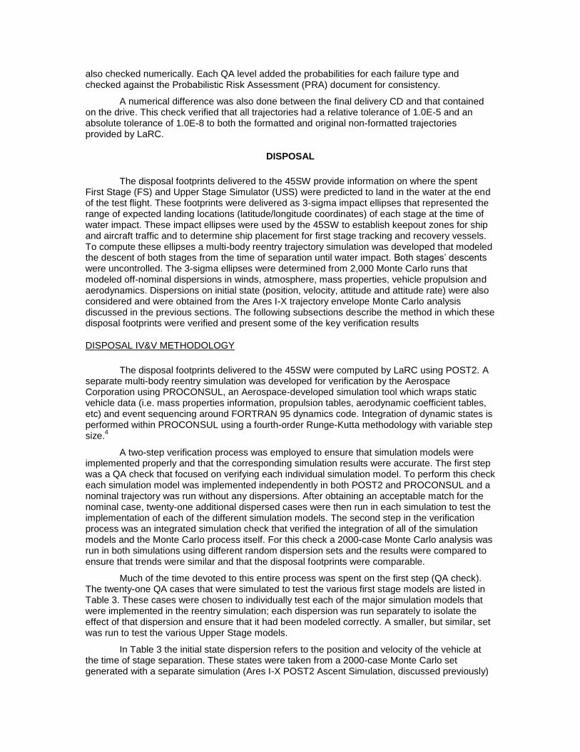
Once all of the QA cases were run, the results from each simulation were compared. Using engineering judgment, a set of metrics was developed to assess the quality of the comparison and to determine if the difference between the disposal footprints determined by each simulation were within the accuracy requirements of the 45SW. The various metrics used to compare simulation results are listed in Table 4. Each metric was computed by differencing results between the two simulations. Two metrics that were considered requirements were developed from the AFSPCMAN 91-710 requirements for radar tracking accuracy that mandated a tracking accuracy of 5% in down range position and 0.5% in cross range position. Since that level of accuracy was acceptable to the 45SW, it was adopted as a QA/IV&V requirement which had to be met before the disposal footprint results could be delivered to the 45SW. As a result, the difference in down range and cross range between the POST2 and PROCONSUL simulations for all of the QA cases had to be less than 5% and 0.5% respectively of the total range of the nominal trajectory (~113 nm). The other metrics listed in the table were treated as guidelines that,

when met, increased confidence in the correctness of the simulations. While there was no strict requirement on meeting these guidelines, in practice, simulation development continued within an allowable timeframe to meet schedule until each QA case satisfied all of the metrics. There was a single QA case that did not meet one of the guideline metrics, but because the reason for the violation was understood and did not impact the disposal footprint accuracy, it was considered acceptable.

Table 4 Quality Assurance Verification Metrics and Nominal Case Results

Metric Do Not

Exceed Value Nominal

Case

*First Stage Down Range at Drogue Deploy within 5% of total down range (nm)

5.00 –0.13

*First Stage Cross Range at Drogue Deploy within 5% of total down range (nm)

2.50 –0.01

Total Angle-of-Attack Profiles within 15 deg 15.00 0.39

Trim attitude at drogue deploy within 5 deg 5.00 –0.02

RSS of pitch and yaw rate profile within 10 deg/s 10.00 0.24

Altitude profiles within 2% 2.00 0.09

Flight path angle profiles within 1 deg 1.00 0.02

Heading angle profile within 1 deg 1.00 0.11

Dynamic pressure profiles within 10% of maximum value 10.00 –0.09

Mach at max. dynamic pressure within 0.1 0.10 0.00

Angle of Attack after stage separation (t = 3 sec) within 0.25 deg 0.25 0.00

Sideslip angle after stage separation (t = 3 sec) within 0.25 deg 0.25 0.00

Pitch rate after tumble motor burn (t = 6 sec) within 0.25 deg/s 0.25 0.00

Yaw rate after tumble motor burn (t = 6 sec) within 0.25 deg/s 0.25 0.00

Roll rate after tumble motor burn (t = 6 sec) within 0.25 deg/s 0.25 0.00

Time to reach end of aerodynamic interference zone within 1 sec 1.00 0.01

Once the QA process was completed, a full Monte Carlo analysis was performed in both simulations. Checks were made for consistency between POST2 and PROCONSUL for a number of key statistical results, the most important of which were the disposal footprints.

DISPOSAL IV&V RESULTS

Staging of the Ares I-X FTV nominally occurs near Mach 4.6 at an altitude of approximately 130,000. At staging, eight booster deceleration motors (BDMs) on FS are ignited and act to reduce the velocity of the FS relative to the USS. After separation the aerodynamically unstable USS begins to tumble as it descends to water impact. Three seconds after staging four booster tumble motors (BTMs) mounted on the FS are ignited to induce a tumbling motion predominantly about the negative yaw-axis. For the first 15-20 sec after staging, the FS is in the wake of the USS and thus is subjected to aerodynamic interference effects. The FS reaches an apogee altitude of ~150,000 ft roughly 40 sec after staging and maximum dynamic pressure (max. q) ~120 sec after staging. For a nominal separation trajectory, the FS reaches max-q

conditions at a total angle-of-attack (T) between 40 and 140 deg (referred to as a “broad-side” entry). This attitude is desired at max-q because it results in the lowest peak dynamic pressure

levels. For some off-nominal conditions it is possible for the FS to have a nose-first (0 deg < T <

40 deg) or tail-first (140 deg < T < 180 deg) attitude at max-q. These trim attitudes are less desirable since they result in larger peak dynamic pressure levels (especially in the case of a nose-first reentry). The probability of each of these three trim attitudes occurring during reentry given the range of off-nominal dispersions was a key pre-flight Monte Carlo result that was compared in both POST2 and PROCONSUL as part of the verification process.

Once the FS descends to an altitude of 16,500 ft, drogue parachutes are deployed. When the FS reaches an altitude of 4,500 ft, the drogues are released and the main parachutes further decelerate the FS to an impact velocity of ~71 ft/sec. The entire parachute sequence from drogue deployment to water impact takes roughly 60-65 sec.

Due to time limitations, the parachute sequence was only modeled in the POST2 simulation. Parachute modeling in POST2 was verified by comparison to a different simulation (not PROCONSUL) and that verification is not discussed here. However, since the FS descended nearly vertical from the time of drogue deploy, the footprint at 16,500 ft was well within 0.01 deg in longitude and latitude to the footprint at water impact. Thus, for the purposes of this range safety verification, the simulation comparison ended at an altitude of 16,500 ft. The disposal footprints that were ultimately delivered to the 45SW were computed by POST2 and did include the parachute deploy sequence.

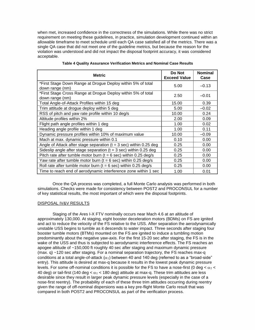
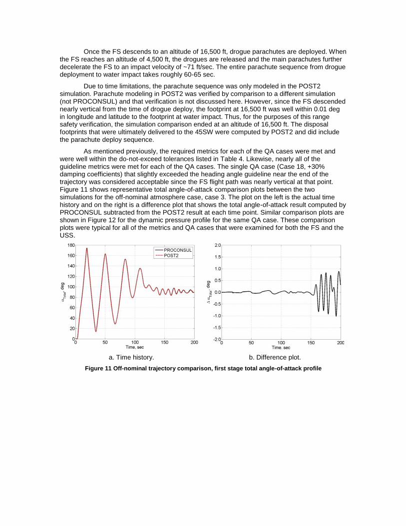
As mentioned previously, the required metrics for each of the QA cases were met and were well within the do-not-exceed tolerances listed in Table 4. Likewise, nearly all of the guideline metrics were met for each of the QA cases. The single QA case (Case 18, +30% damping coefficients) that slightly exceeded the heading angle guideline near the end of the trajectory was considered acceptable since the FS flight path was nearly vertical at that point. Figure 11 shows representative total angle-of-attack comparison plots between the two simulations for the off-nominal atmosphere case, case 3. The plot on the left is the actual time history and on the right is a difference plot that shows the total angle-of-attack result computed by PROCONSUL subtracted from the POST2 result at each time point. Similar comparison plots are shown in Figure 12 for the dynamic pressure profile for the same QA case. These comparison plots were typical for all of the metrics and QA cases that were examined for both the FS and the USS.

a. Time history. b. Difference plot.

Figure 11 Off-nominal trajectory comparison, first stage total angle-of-attack profile

a. Time history. b. Difference plot.

Figure 12 Off-nominal trajectory comparison, first stage dynamic pressure profile

After successfully completing the QA verification, a final Monte Carlo analysis comparison was performed using the full set of simulation model dispersions that were tested individually in the QA verification. For this comparison, 2,000 Monte Carlo cases that randomly perturbed all of the dispersions simultaneously were run in both POST2 and PROCONSUL using the distribution for each dispersion. While the random distributions were the same, the actual dispersed parameter values used in each perturbed case differed in each simulation. Overall, the level of agreement in the statistical results generated by each simulation was excellent. A representative example of the statistical results from each simulation is shown in Table 5, which compares the 50 and 97.7 percentile values of key parameters at the time of maximum dynamic pressure. The statistics at maximum dynamic pressure were not required by the 45SW but were important to the test flight program and needed to be quantified prior to flight to estimate the critical loads occurred that occur then.

Also shown in Table 5 is the percentage of the 2,000 cases that had a trim attitude at max-q that was nose-first, broad-side or tail-first, respectively. Due to peak loading concerns a broad-side max-q trim attitude was desirable, a tail-first was tolerable and a nose-first would result in drogue deployment failure. The results presented in Table 5 were conservative since they used worst-case center-of-gravity location assumptions. Again, there is very good agreement between the results generated by each code.

Table 5 First stage Monte Carlo statistics comparison at maximum dynamic pressure

50 Percentile 97.7 Percentile

At Max. Dynamic Pressure POST2 PROCONSUL POST2 PROCONSUL

Dynamic Pressure, psf 495 505 3589 3596

Total Angle-of-Attack, deg 111.4 113.0 155.7 155.9

Mach number 2.61 2.60 3.38 3.37

Altitude, kft 66.85 65.57 84.42 84.29

Percent Nose-First 18.75 18.36

Percent Broad-Side 62.15 62.98

Percent Tail-First 19.10 18.66

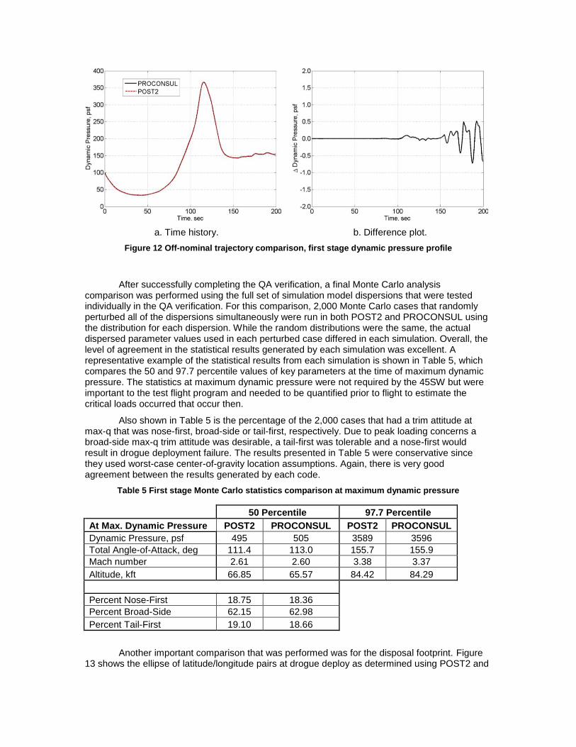
Another important comparison that was performed was for the disposal footprint. Figure 13 shows the ellipse of latitude/longitude pairs at drogue deploy as determined using POST2 and

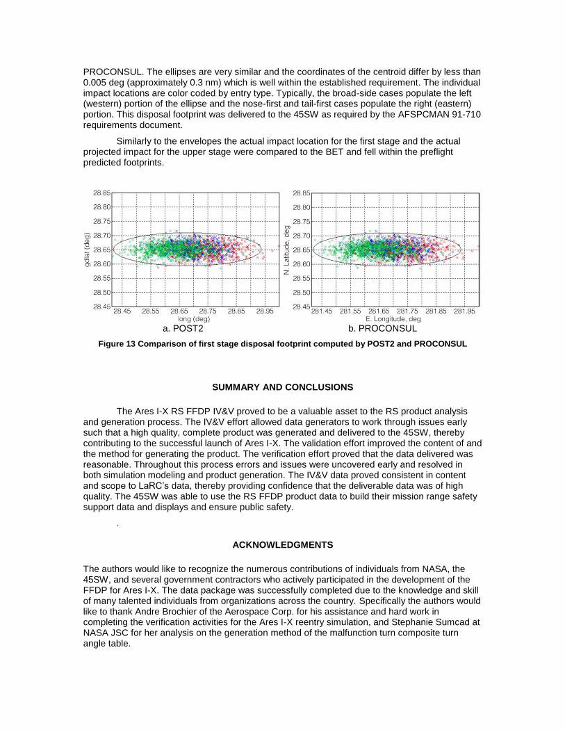
PROCONSUL. The ellipses are very similar and the coordinates of the centroid differ by less than 0.005 deg (approximately 0.3 nm) which is well within the established requirement. The individual impact locations are color coded by entry type. Typically, the broad-side cases populate the left (western) portion of the ellipse and the nose-first and tail-first cases populate the right (eastern) portion. This disposal footprint was delivered to the 45SW as required by the AFSPCMAN 91-710 requirements document.

Similarly to the envelopes the actual impact location for the first stage and the actual projected impact for the upper stage were compared to the BET and fell within the preflight predicted footprints.

a. POST2 b. PROCONSUL

Figure 13 Comparison of first stage disposal footprint computed by POST2 and PROCONSUL

SUMMARY AND CONCLUSIONS

The Ares I-X RS FFDP IV&V proved to be a valuable asset to the RS product analysis and generation process. The IV&V effort allowed data generators to work through issues early such that a high quality, complete product was generated and delivered to the 45SW, thereby contributing to the successful launch of Ares I-X. The validation effort improved the content of and the method for generating the product. The verification effort proved that the data delivered was reasonable. Throughout this process errors and issues were uncovered early and resolved in both simulation modeling and product generation. The IV&V data proved consistent in content and scope to LaRC’s data, thereby providing confidence that the deliverable data was of high quality. The 45SW was able to use the RS FFDP product data to build their mission range safety support data and displays and ensure public safety.

.

ACKNOWLEDGMENTS

The authors would like to recognize the numerous contributions of individuals from NASA, the 45SW, and several government contractors who actively participated in the development of the FFDP for Ares I-X. The data package was successfully completed due to the knowledge and skill of many talented individuals from organizations across the country. Specifically the authors would like to thank Andre Brochier of the Aerospace Corp. for his assistance and hard work in completing the verification activities for the Ares I-X reentry simulation, and Stephanie Sumcad at NASA JSC for her analysis on the generation method of the malfunction turn composite turn angle table.

REFERENCES

1. Starr, Brett R., et.al., “Ares I-X Range Safety Three Sigma Trajectory Envelope Analysis, ” JANNAF Propulsion Meeting, Arlington, VA, April 18-22, 2011. 2. Beaty, James R., “Ares I-X Malfunction Turn Range Safety Analysis,” JANNAF Propulsion Meeting, Arlington, VA, April 18-22, 2011. 3. Starr, Brett R. et.al., “Ares I-X Range Safety Overview,” JANNAF Propulsion Meeting, Arlington, VA, April 18-22, 2011. 4. A. Brochier, C. Heidelberger, "Ares I-X Reentry Analysis," Aerospace Corporation, ATR-2009(5472)-17, August 26 2009. 5. Justus, C.G., F.W. Leslie, “The NASA MSFC Earth Global Reference Atmospheric Model – 2007 Version”, NASA TM 2008-215581, November 2008.

GLOSSARY

45SW = 45th Space Wing

6DOF = 6 Degrees-of-Freedom

AFSPCMAN = Air Force Space Command Manual

DOLILU = Day-of-Launch I-Load Update

ANTARES = Advanced NASA Technology Architecture for Exploration Studies

ATK = Alliant Techsystems Inc.

BDM = Booster Deceleration Motors

BTM = Booster Tumble Motors

FFDP = Final Flight Data Package

FFPA = Final Flight Plan Approval

FS = First Stage

FTV = Flight Test Vehicle

IV&V = Independent Validation and Verification

JSC = Johnson Space Center

LaRC = Langley Research Center

LCRSP = Launch Constellation Range Safety Panel

MAVERIC = Marshall Aerospace Vehicle Representation In C

MFCO = Mission Flight Control Officer

MSFC = Marshall Space Flight Center

MT = Malfunction Turn

PFPA = Preliminary Flight Plan Approval

POST2 = Program to Optimize Simulated Trajectories II

PROCONSUL = Programmer's Continuous Simulation Tool

QA = Quality Assurance

RS = Range Safety

RSTWG = Range Safety Trajectory Working Group

SE&I = Systems Engineering and Integration

SSP = Space Shuttle Program

USS = Upper Stage Simulator

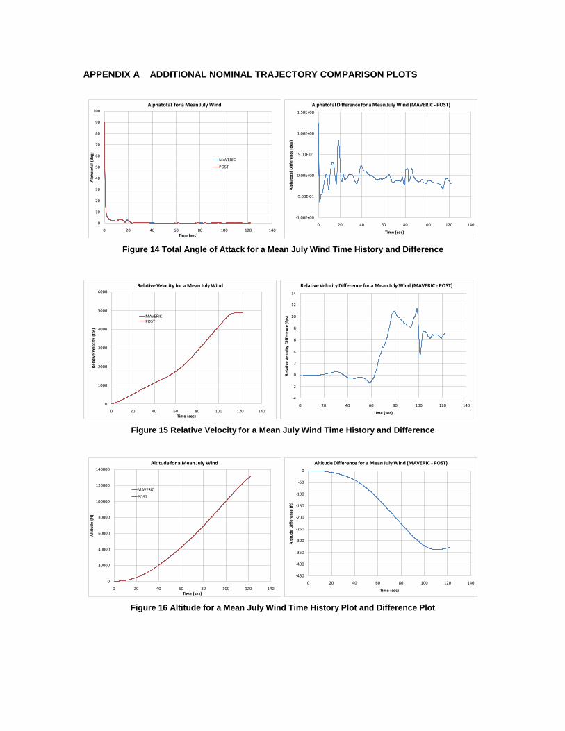
APPENDIX A ADDITIONAL NOMINAL TRAJECTORY COMPARISON PLOTS

0

10

20

30

40

50

60

70

80

90

100

0 20 40 60 80 100 120 140

Alp

hat

ota

l (d

eg)

Time (sec)

Alphatotal for a Mean July Wind

MAVERIC

POST

-1.00E+00

-5.00E-01

0.00E+00

5.00E-01

1.00E+00

1.50E+00

0 20 40 60 80 100 120 140

Alp

hat

ota

l D

iffe

ren

ce (d

eg)

Time (sec)

Alphatotal Difference for a Mean July Wind (MAVERIC - POST)

Figure 14 Total Angle of Attack for a Mean July Wind Time History and Difference

0

1000

2000

3000

4000

5000

6000

0 20 40 60 80 100 120 140

Re

lati

ve V

elo

city

(fp

s)

Time (sec)

Relative Velocity for a Mean July Wind

MAVERICPOST

-4

-2

0

2

4

6

8

10

12

14

0 20 40 60 80 100 120 140

Re

lati

ve V

elo

city

Dif

fere

nce

(fp

s)

Time (sec)

Relative Velocity Difference for a Mean July Wind (MAVERIC - POST)

Figure 15 Relative Velocity for a Mean July Wind Time History and Difference

0

20000

40000

60000

80000

100000

120000

140000

0 20 40 60 80 100 120 140

Alt

itu

de

(ft

)

Time (sec)

Altitude for a Mean July Wind

MAVERIC

POST

-450

-400

-350

-300

-250

-200

-150

-100

-50

0

0 20 40 60 80 100 120 140

Alt

itu

de

Dif

fere

nce

(ft)

Time (sec)

Altitude Difference for a Mean July Wind (MAVERIC - POST)

Figure 16 Altitude for a Mean July Wind Time History Plot and Difference Plot

-40

-20

0

20

40

60

80

100

120

0 20 40 60 80 100 120 140

Flig

ht

Pat

h A

ngl

e (

de

g)

Time (sec)

Flight Path Angle for a Mean July Wind

MAVERIC

POST

-1

-0.8

-0.6

-0.4

-0.2

0

0.2

0.4

0.6

0.8

1

0 20 40 60 80 100 120 140

FPA

Dif

fere

nce

(d

eg)

Time (sec)

Flight Path Angle Difference for a Mean July Wind (MAVERIC - POST)

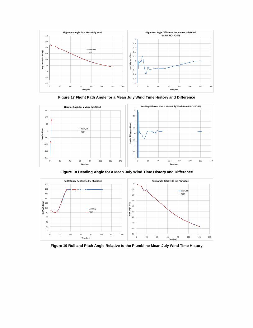
Figure 17 Flight Path Angle for a Mean July Wind Time History and Difference

-200

-150

-100

-50

0

50

100

150

0 20 40 60 80 100 120 140

He

adin

g (d

eg)

Time (sec)

Heading Angle for a Mean July Wind

MAVERIC

POST

-2

-1.5

-1

-0.5

0

0.5

1

1.5

2

0 20 40 60 80 100 120 140

He

adin

g D

iffe

ren

ce (d

eg)

Time (sec)

Heading Difference for a Mean July Wind (MAVERIC - POST)

Figure 18 Heading Angle for a Mean July Wind Time History and Difference

0

20

40

60

80

100

120

140

160

180

200

0 20 40 60 80 100 120 140

Ro

ll A

ngl

e (

de

g)

Time (sec)

Roll Attitude Relative to the Plumbline

MAVERIC

POST

-90

-80

-70

-60

-50

-40

-30

-20

-10

0

0 20 40 60 80 100 120 140

Pit

ch A

ngl

e (

de

g)

Time (sec)

Pitch Angle Relative to the Plumbline

MAVERIC

POST

Figure 19 Roll and Pitch Angle Relative to the Plumbline Mean July Wind Time History

-2

-1.5

-1

-0.5

0

0.5

1

1.5

0 20 40 60 80 100 120 140

Yaw

An

gle

(d

eg)

Time (sec)

Yaw Attitude Relative to the Plumbline

MAVERIC

POST

-5

-4

-3

-2

-1

0

1

2

0 20 40 60 80 100 120 140

Dif

fere

nce

in A

ngl

es

(de

g)

Time (sec)

Differences in Vehicle Attitude (MAVERIC - POST)

Roll

Pitch

Yaw

Figure 20 Yaw Angle Relative to the Plumbline Mean July Wind Time History and the Difference for the Attitudes Relative to the Plumbline

28.625

28.63

28.635

28.64

28.645

28.65

28.655

28.66

279 279.5 280 280.5 281 281.5 282 282.5

Lati

tud

e (

de

g)

Longitude (deg)

Instantaneous Impact Points for a Mean July Wind

MAVERICPOST

-0.008

-0.007

-0.006

-0.005

-0.004

-0.003

-0.002

-0.001

0

0.001

279 279.5 280 280.5 281 281.5 282 282.5

Lati

tud

e I

IP D

iffe

ren

ce(d

eg)

Longitude (deg)

Latitude IIP Difference for a Mean July Wind (MAVERIC - POST)

Figure 21 IIP’s for a Mean July Wind and Difference Plot

0

100

200

300

400

500

600

700

800

900

1000

0 1 2 3 4 5

Dyn

amic

Pre

ssu

re (

psf

)

Mach

Dynamic Pressure vs Mach for a Mean July Wind

MAVERIC

POST

Figure 22 Mach vs Dynamic Pressure for MAVERIC and POST2

APPENDIX B ADDITIONAL DISPERSED TRAJECTORY COMPARISON PLOTS

Figure 23 POST and MAVERIC dispersion plots for the LAS trajectory

Figure 24 POST and MAVERIC dispersion plots for the LAL trajectory

POST2 MAVERIC

Figure 25 POST and MAVERIC dispersion plots for the Minimum IIP

POST2

MAVERIC

POST2

MAVERIC

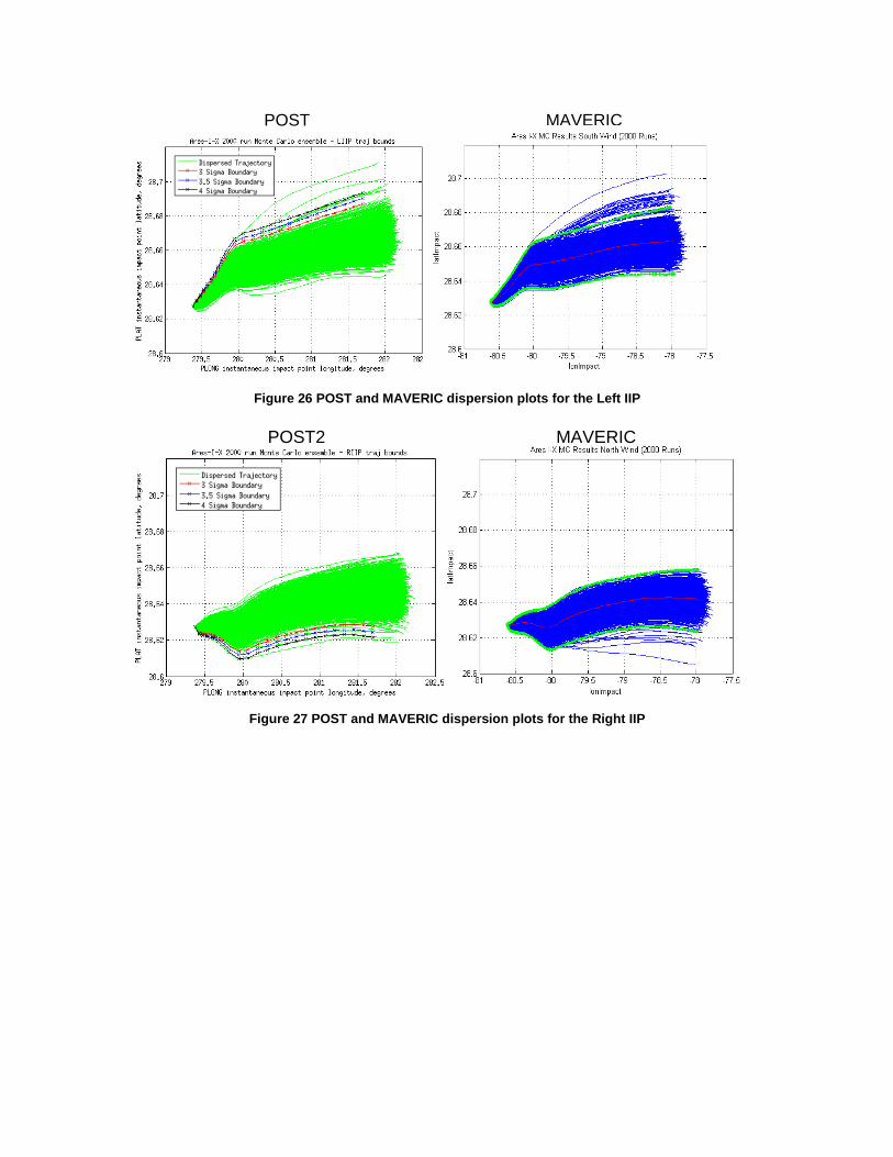
Figure 26 POST and MAVERIC dispersion plots for the Left IIP

Figure 27 POST and MAVERIC dispersion plots for the Right IIP

POST2 MAVERIC

POST2

MAVERIC

APPENDIX C ADDITIONAL ENVELOPE TRAJECTORY COMPARISON PLOTS

0

20000

40000

60000

80000

100000

120000

140000

0 20000 40000 60000 80000 100000 120000 140000 160000 180000

Zvrt

(ft

)

Yvrt (ft)

LAL

MAVERIC LAL

MAVERIC nominal

POST LAL

0

20000

40000

60000

80000

100000

120000

140000

0 50000 100000 150000 200000 250000

Zvrt

(ft

)

Xvrt (ft)

LAS

MAVERIC LAS

MAVERIC nominal

POST LAS

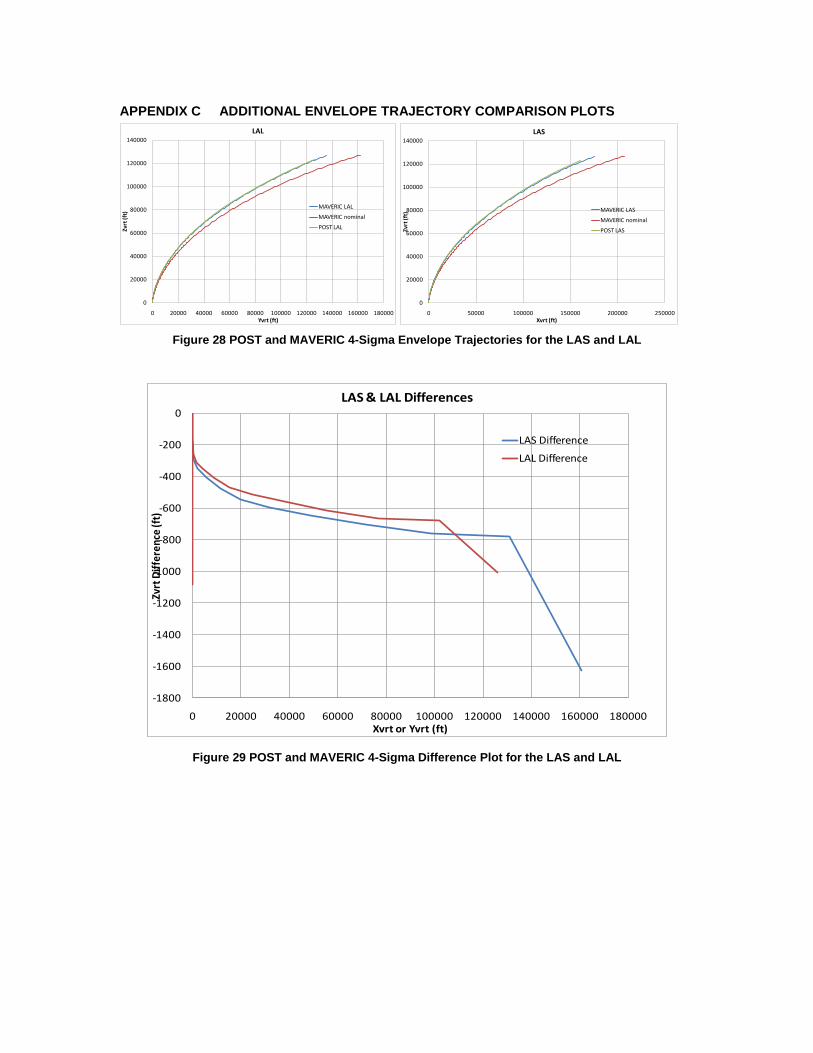
Figure 28 POST and MAVERIC 4-Sigma Envelope Trajectories for the LAS and LAL

-1800

-1600

-1400

-1200

-1000

-800

-600

-400

-200

0

0 20000 40000 60000 80000 100000 120000 140000 160000 180000

Zvrt

Dif

fere

nce

(ft)

Xvrt or Yvrt (ft)

LAS & LAL Differences

LAS Difference

LAL Difference

Figure 29 POST and MAVERIC 4-Sigma Difference Plot for the LAS and LAL

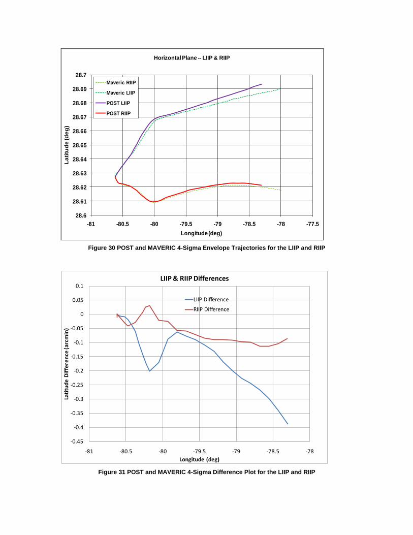
28.6

28.61

28.62

28.63

28.64

28.65

28.66

28.67

28.68

28.69

28.7

-81 -80.5 -80 -79.5 -79 -78.5 -78 -77.5

La

titu

de

(d

eg

)

Longitude (deg)

Horizontal Plane -- LIIP & RIIP

Maveric RIIP

Maveric LIIP

POST LIIP

POST RIIP

Figure 30 POST and MAVERIC 4-Sigma Envelope Trajectories for the LIIP and RIIP

-0.45

-0.4

-0.35

-0.3

-0.25

-0.2

-0.15

-0.1

-0.05

0

0.05

0.1

-81 -80.5 -80 -79.5 -79 -78.5 -78

Lati

tud

e D

iffe

ren

ce (a

rcm

in)

Longitude (deg)

LIIP & RIIP Differences

LIIP Difference

RIIP Difference

Figure 31 POST and MAVERIC 4-Sigma Difference Plot for the LIIP and RIIP

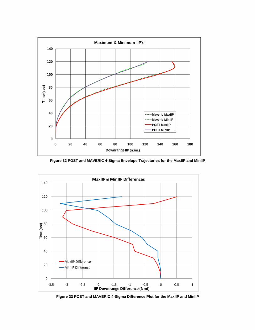
0

20

40

60

80

100

120

140

0 20 40 60 80 100 120 140 160 180

Tim

e (s

ec

)

Downrange IIP (n.mi.)

Maximum & Minimum IIP's

Maveric MaxIIP

Maveric MinIIP

POST MaxIIP

POST MinIIP

Figure 32 POST and MAVERIC 4-Sigma Envelope Trajectories for the MaxIIP and MinIIP

0

20

40

60

80

100

120

140

-3.5 -3 -2.5 -2 -1.5 -1 -0.5 0 0.5 1

Tim

e (

sec)

IIP Downrange Difference (Nmi)

MaxIIP & MinIIP Differences

MaxIIP Difference

MinIIP Difference

Figure 33 POST and MAVERIC 4-Sigma Difference Plot for the MaxIIP and MinIIP

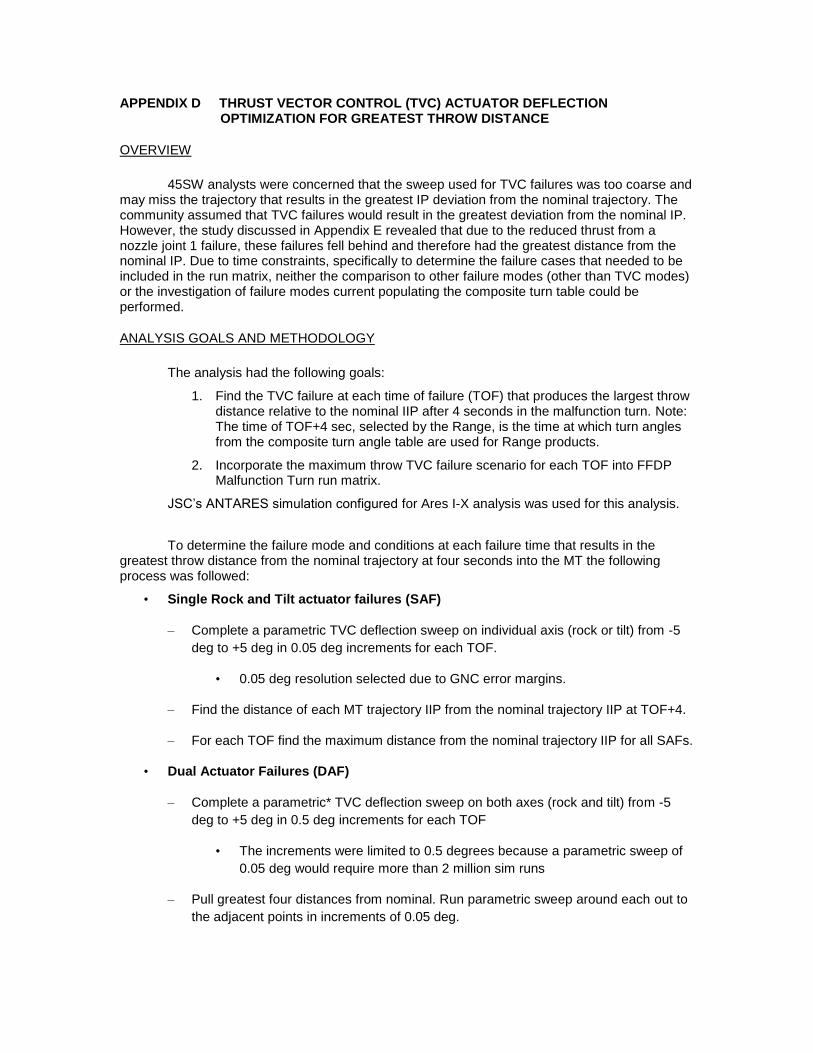
APPENDIX D THRUST VECTOR CONTROL (TVC) ACTUATOR DEFLECTION OPTIMIZATION FOR GREATEST THROW DISTANCE

OVERVIEW

45SW analysts were concerned that the sweep used for TVC failures was too coarse and may miss the trajectory that results in the greatest IP deviation from the nominal trajectory. The community assumed that TVC failures would result in the greatest deviation from the nominal IP. However, the study discussed in Appendix E revealed that due to the reduced thrust from a nozzle joint 1 failure, these failures fell behind and therefore had the greatest distance from the nominal IP. Due to time constraints, specifically to determine the failure cases that needed to be included in the run matrix, neither the comparison to other failure modes (other than TVC modes) or the investigation of failure modes current populating the composite turn table could be performed.

ANALYSIS GOALS AND METHODOLOGY

The analysis had the following goals:

1. Find the TVC failure at each time of failure (TOF) that produces the largest throw distance relative to the nominal IIP after 4 seconds in the malfunction turn. Note: The time of TOF+4 sec, selected by the Range, is the time at which turn angles from the composite turn angle table are used for Range products.

2. Incorporate the maximum throw TVC failure scenario for each TOF into FFDP Malfunction Turn run matrix.

JSC’s ANTARES simulation configured for Ares I-X analysis was used for this analysis.

To determine the failure mode and conditions at each failure time that results in the

greatest throw distance from the nominal trajectory at four seconds into the MT the following process was followed:

• Single Rock and Tilt actuator failures (SAF)

– Complete a parametric TVC deflection sweep on individual axis (rock or tilt) from -5

deg to +5 deg in 0.05 deg increments for each TOF.

• 0.05 deg resolution selected due to GNC error margins.

– Find the distance of each MT trajectory IIP from the nominal trajectory IIP at TOF+4.

– For each TOF find the maximum distance from the nominal trajectory IIP for all SAFs.

• Dual Actuator Failures (DAF)

– Complete a parametric* TVC deflection sweep on both axes (rock and tilt) from -5

deg to +5 deg in 0.5 deg increments for each TOF

• The increments were limited to 0.5 degrees because a parametric sweep of

0.05 deg would require more than 2 million sim runs

– Pull greatest four distances from nominal. Run parametric sweep around each out to

the adjacent points in increments of 0.05 deg.

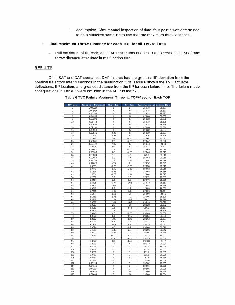
• Assumption: After manual inspection of data, four points was determined

to be a sufficient sampling to find the true maximum throw distance.

• Final Maximum Throw Distance for each TOF for all TVC failures

– Pull maximum of tilt, rock, and DAF maximums at each TOF to create final list of max

throw distance after 4sec in malfunction turn.

RESULTS

Of all SAF and DAF scenarios, DAF failures had the greatest IIP deviation from the nominal trajectory after 4 seconds in the malfunction turn. Table 6 shows the TVC actuator deflections, IIP location, and greatest distance from the IIP for each failure time. The failure mode configurations in Table 6 were included in the MT run matrix.

Table 6 TVC Failure Maximum Throw at TOF+4sec for Each TOF

TOF (sec) Range from Nom (nmi) Rock (deg) Tilt (deg) Longitude (deg) Latitude (deg)

0 0.030385 5 5 279.38 28.627

2 0.071416 -5 -5 279.38 28.627

4 0.10392 -5 -5 279.38 28.627

6 0.14955 -5 -5 279.38 28.627

8 0.22309 -5 -5 279.38 28.628

10 0.26758 -5 -5 279.38 28.628

12 0.32509 -5 -5 279.38 28.628

14 0.37138 -5 -5 279.38 28.628

16 0.48948 -5 -5 279.39 28.627

18 0.69566 -4.25 -5 279.39 28.627

20 0.7196 -3.95 -5 279.4 28.625

22 0.7441 -3.7 -4.75 279.41 28.623

24 0.78381 -2.9 -4.85 279.42 28.622

26 0.82402 2.15 -5 279.43 28.63

28 0.8594 -0.8 -5 279.44 28.622

30 0.89612 -1.2 -4.65 279.46 28.619

32 0.93309 -0.8 -4.55 279.48 28.619

34 0.93394 -1.3 -4.1 279.5 28.618

36 0.89849 -1.5 -3.6 279.52 28.618

38 0.91769 -1.3 -3.5 279.54 28.619

40 0.97075 3.75 1 279.57 28.645

42 1.0308 -1.25 -3.35 279.59 28.619

44 1.0748 -1.45 -3.15 279.62 28.618

46 1.1215 -1.65 -3 279.65 28.618

48 1.175 -1.75 -2.9 279.68 28.617

50 1.2501 3.2 1.3 279.71 28.653

52 1.3464 2.8 1.8 279.75 28.656

54 1.4428 2.75 1.65 279.79 28.657

56 1.5321 2.65 1.6 279.83 28.659

58 1.6513 2.5 1.7 279.88 28.662

60 1.7859 2.45 1.7 279.93 28.664

62 1.956 -1.65 -2 279.98 28.61

64 2.1463 -1.65 -2.1 280.04 28.609

66 2.3713 2.35 1.85 280.1 28.675

68 2.6236 2.45 1.85 280.16 28.679

70 2.9012 -2.2 -2 280.23 28.602

72 3.2083 2.2 2.45 280.3 28.687

74 3.5379 -2.5 -2.1 280.38 28.598

76 3.8146 -2.9 -1.85 280.46 28.598

78 4.0206 1.9 3.15 280.54 28.695

80 4.2517 1.85 3.35 280.63 28.697

82 4.5033 1.6 3.7 280.71 28.697

84 4.7487 0.65 4.2 280.79 28.691

86 5.0274 -4.5 0.7 280.88 28.618

88 5.4618 -3.85 2.8 280.96 28.642

90 5.9372 -3.25 3.8 281.05 28.655

92 6.3528 -2.75 4.5 281.14 28.665

94 6.7333 -3.55 4.25 281.23 28.658

96 6.8322 -3.4 4.45 281.33 28.661

98 6.8865 -4.1 4 281.43 28.653

100 8.235 -5 5 281.5 28.654

102 8.0784 -5 5 281.6 28.655

104 7.8551 -5 5 281.7 28.655

106 6.8707 -5 5 281.8 28.655

108 4.5997 -5 5 281.9 28.656

110 2.2872 -5 5 281.98 28.656

112 0.98124 -5 5 282.02 28.655

114 0.34115 -5 5 282.05 28.655

116 0.065327 -5 5 282.06 28.655

118 0.022279 5 -5 282.06 28.654

120 0.01669 5 -5 282.06 28.654

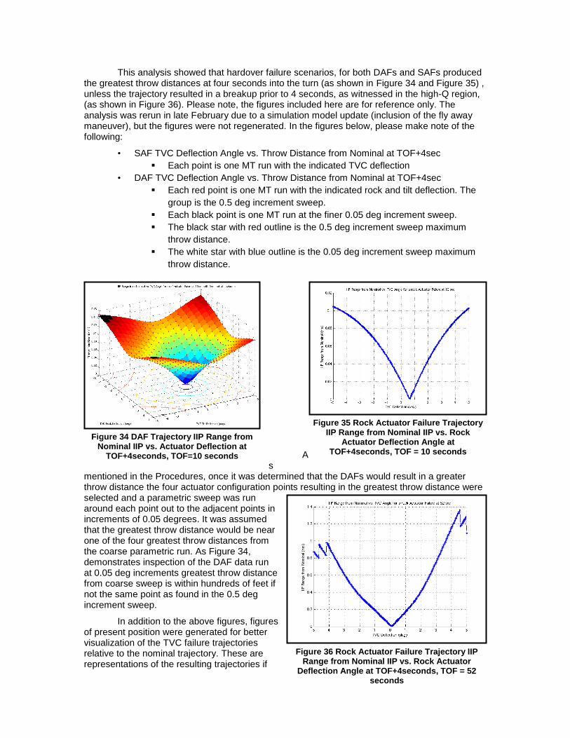
This analysis showed that hardover failure scenarios, for both DAFs and SAFs produced the greatest throw distances at four seconds into the turn (as shown in Figure 34 and Figure 35) , unless the trajectory resulted in a breakup prior to 4 seconds, as witnessed in the high-Q region, (as shown in Figure 36). Please note, the figures included here are for reference only. The analysis was rerun in late February due to a simulation model update (inclusion of the fly away maneuver), but the figures were not regenerated. In the figures below, please make note of the following:

• SAF TVC Deflection Angle vs. Throw Distance from Nominal at TOF+4sec

Each point is one MT run with the indicated TVC deflection

• DAF TVC Deflection Angle vs. Throw Distance from Nominal at TOF+4sec

Each red point is one MT run with the indicated rock and tilt deflection. The

group is the 0.5 deg increment sweep.

Each black point is one MT run at the finer 0.05 deg increment sweep.

The black star with red outline is the 0.5 deg increment sweep maximum

throw distance.

The white star with blue outline is the 0.05 deg increment sweep maximum

throw distance.

As

mentioned in the Procedures, once it was determined that the DAFs would result in a greater throw distance the four actuator configuration points resulting in the greatest throw distance were selected and a parametric sweep was run around each point out to the adjacent points in increments of 0.05 degrees. It was assumed that the greatest throw distance would be near one of the four greatest throw distances from the coarse parametric run. As Figure 34, demonstrates inspection of the DAF data run at 0.05 deg increments greatest throw distance from coarse sweep is within hundreds of feet if not the same point as found in the 0.5 deg increment sweep.

In addition to the above figures, figures of present position were generated for better visualization of the TVC failure trajectories relative to the nominal trajectory. These are representations of the resulting trajectories if

Figure 35 Rock Actuator Failure Trajectory IIP Range from Nominal IIP vs. Rock

Actuator Deflection Angle at TOF+4seconds, TOF = 10 seconds

Figure 34 DAF Trajectory IIP Range from Nominal IIP vs. Actuator Deflection at

TOF+4seconds, TOF=10 seconds

Figure 36 Rock Actuator Failure Trajectory IIP Range from Nominal IIP vs. Rock Actuator

Deflection Angle at TOF+4seconds, TOF = 52 seconds

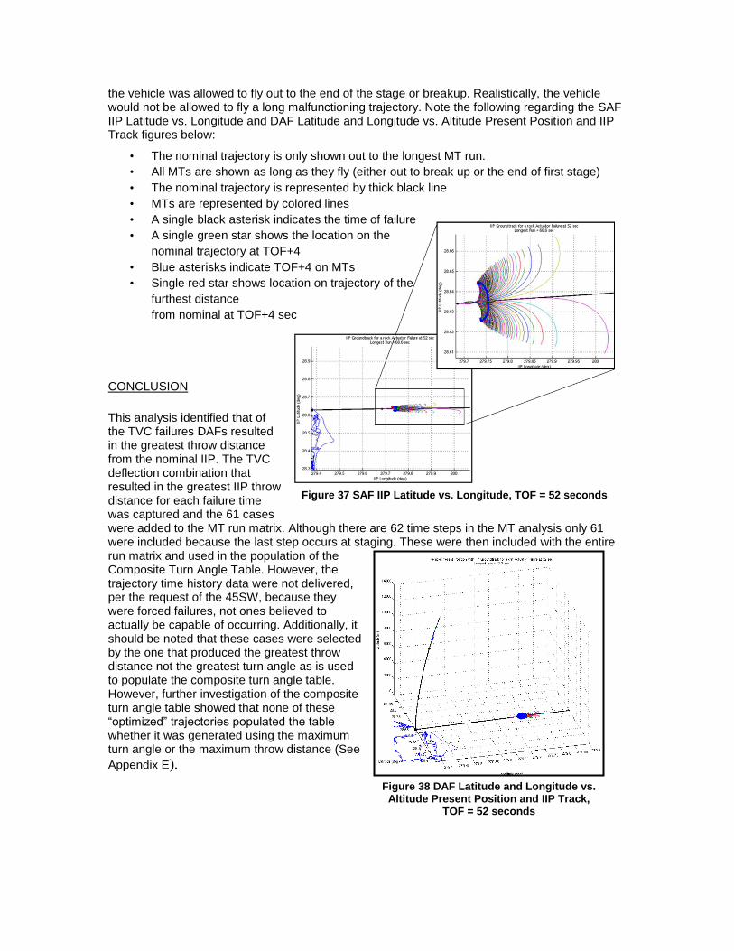
Figure 37 SAF IIP Latitude vs. Longitude, TOF = 52 seconds

the vehicle was allowed to fly out to the end of the stage or breakup. Realistically, the vehicle would not be allowed to fly a long malfunctioning trajectory. Note the following regarding the SAF IIP Latitude vs. Longitude and DAF Latitude and Longitude vs. Altitude Present Position and IIP Track figures below:

• The nominal trajectory is only shown out to the longest MT run.

• All MTs are shown as long as they fly (either out to break up or the end of first stage)

• The nominal trajectory is represented by thick black line

• MTs are represented by colored lines

• A single black asterisk indicates the time of failure

• A single green star shows the location on the

nominal trajectory at TOF+4

• Blue asterisks indicate TOF+4 on MTs

• Single red star shows location on trajectory of the

furthest distance

from nominal at TOF+4 sec

CONCLUSION

This analysis identified that of the TVC failures DAFs resulted in the greatest throw distance from the nominal IIP. The TVC deflection combination that resulted in the greatest IIP throw distance for each failure time was captured and the 61 cases were added to the MT run matrix. Although there are 62 time steps in the MT analysis only 61 were included because the last step occurs at staging. These were then included with the entire run matrix and used in the population of the Composite Turn Angle Table. However, the trajectory time history data were not delivered, per the request of the 45SW, because they were forced failures, not ones believed to actually be capable of occurring. Additionally, it should be noted that these cases were selected by the one that produced the greatest throw distance not the greatest turn angle as is used to populate the composite turn angle table. However, further investigation of the composite turn angle table showed that none of these “optimized” trajectories populated the table whether it was generated using the maximum turn angle or the maximum throw distance (See

Appendix E).

Figure 38 DAF Latitude and Longitude vs. Altitude Present Position and IIP Track,

TOF = 52 seconds

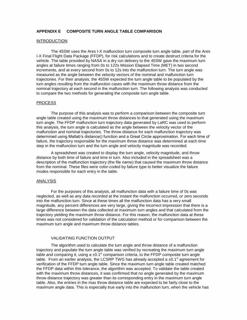
APPENDIX E COMPOSITE TURN ANGLE TABLE COMPARISON

INTRODUCTION

The 45SW uses the Ares I-X malfunction turn composite turn angle table, part of the Ares I-X Final Flight Data Package (FFDP), for risk calculations and to create destruct criteria for the vehicle. The table provided by NASA in a dry run delivery to the 45SW gave the maximum turn angles at failure times ranging from 0s to 122s Mission Elapsed Time (MET) in two second increments, and at every second from 0s to 12s into the malfunction turn. The turn angle was measured as the angle between the velocity vectors of the nominal and malfunction turn trajectories. For their analysis, the 45SW expected the turn angle table to be populated by the turn angles resulting from the malfunction cases with the maximum throw distance from the nominal trajectory at each second in the malfunction turn. The following analysis was conducted to compare the two methods for generating the composite turn angle table.

PROCESS

The purpose of this analysis was to perform a comparison between the composite turn angle table created using the maximum throw distances to that generated using the maximum turn angle. The FFDP malfunction turn trajectory data generated by LaRC was used to perform this analysis, the turn angle is calculated as the angle between the velocity vector of the malfunction and nominal trajectories. The throw distance for each malfunction trajectory was determined using Matlab’s distance() function and a Great Circle approximation. For each time of failure, the trajectory responsible for the maximum throw distance was determined at each time step in the malfunction turn and the turn angle and velocity magnitude was recorded.

A spreadsheet was created to display the turn angle, velocity magnitude, and throw distance by both time of failure and time in turn. Also included in the spreadsheet was a description of the malfunction trajectory (the file name) that caused the maximum throw distance from the nominal. These files were color-coded by failure type to better visualize the failure modes responsible for each entry in the table.

ANALYSIS

For the purposes of this analysis, all malfunction data with a failure time of 0s was neglected, as well as any data recorded at the instant the malfunction occurred, or zero seconds into the malfunction turn. Since at these times all the malfunction data has a very small magnitude, any percent differences are very large, giving the incorrect impression that there is a large difference between the data collected at maximum turn angles and that calculated from the trajectory yielding the maximum throw distance. For this reason, the malfunction data at these times was not considered for validation of the calculation method or for comparison between the maximum turn angle and maximum throw distance tables.

VALIDATING FUNCTION OUTPUT

The algorithm used to calculate the turn angle and throw distance of a malfunction trajectory and populate the turn angle table was verified by recreating the maximum turn angle

table and comparing it, using a ±0.1⁰ comparison criteria, to the FFDP composite turn angle table. From an earlier analysis, the LCSRP TWG has already accepted a ±0.1⁰ agreement for verification of the FFDP turn angle table. Since the maximum turn angle table created matched the FFDP data within this tolerance, the algorithm was accepted. To validate the table created with the maximum throw distances, it was confirmed that no angle generated by the maximum throw distance trajectory was greater than its corresponding entry in the maximum turn angle table. Also, the entries in the max throw distance table are expected to be fairly close to the maximum angle data. This is especially true early into the malfunction turn, when the vehicle has

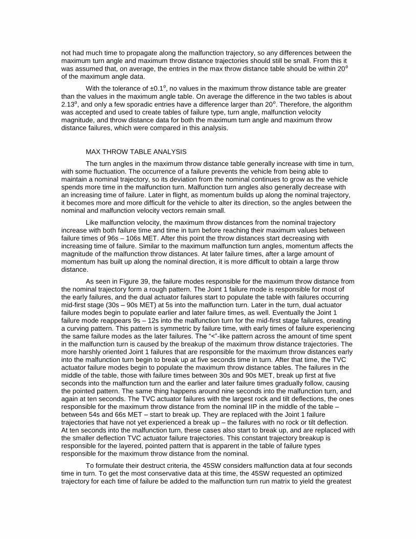
not had much time to propagate along the malfunction trajectory, so any differences between the maximum turn angle and maximum throw distance trajectories should still be small. From this it

was assumed that, on average, the entries in the max throw distance table should be within 20⁰ of the maximum angle data.

With the tolerance of ±0.1⁰, no values in the maximum throw distance table are greater

than the values in the maximum angle table. On average the difference in the two tables is about

2.13⁰, and only a few sporadic entries have a difference larger than 20⁰. Therefore, the algorithm was accepted and used to create tables of failure type, turn angle, malfunction velocity magnitude, and throw distance data for both the maximum turn angle and maximum throw distance failures, which were compared in this analysis.

MAX THROW TABLE ANALYSIS

The turn angles in the maximum throw distance table generally increase with time in turn, with some fluctuation. The occurrence of a failure prevents the vehicle from being able to maintain a nominal trajectory, so its deviation from the nominal continues to grow as the vehicle spends more time in the malfunction turn. Malfunction turn angles also generally decrease with an increasing time of failure. Later in flight, as momentum builds up along the nominal trajectory, it becomes more and more difficult for the vehicle to alter its direction, so the angles between the nominal and malfunction velocity vectors remain small.

Like malfunction velocity, the maximum throw distances from the nominal trajectory increase with both failure time and time in turn before reaching their maximum values between failure times of 96s – 106s MET. After this point the throw distances start decreasing with increasing time of failure. Similar to the maximum malfunction turn angles, momentum affects the magnitude of the malfunction throw distances. At later failure times, after a large amount of momentum has built up along the nominal direction, it is more difficult to obtain a large throw distance.

As seen in Figure 39, the failure modes responsible for the maximum throw distance from the nominal trajectory form a rough pattern. The Joint 1 failure mode is responsible for most of the early failures, and the dual actuator failures start to populate the table with failures occurring mid-first stage (30s – 90s MET) at 5s into the malfunction turn. Later in the turn, dual actuator failure modes begin to populate earlier and later failure times, as well. Eventually the Joint 1 failure mode reappears 9s – 12s into the malfunction turn for the mid-first stage failures, creating a curving pattern. This pattern is symmetric by failure time, with early times of failure experiencing the same failure modes as the later failures. The “<”-like pattern across the amount of time spent in the malfunction turn is caused by the breakup of the maximum throw distance trajectories. The more harshly oriented Joint 1 failures that are responsible for the maximum throw distances early into the malfunction turn begin to break up at five seconds time in turn. After that time, the TVC actuator failure modes begin to populate the maximum throw distance tables. The failures in the middle of the table, those with failure times between 30s and 90s MET, break up first at five seconds into the malfunction turn and the earlier and later failure times gradually follow, causing the pointed pattern. The same thing happens around nine seconds into the malfunction turn, and again at ten seconds. The TVC actuator failures with the largest rock and tilt deflections, the ones responsible for the maximum throw distance from the nominal IIP in the middle of the table – between 54s and 66s MET – start to break up. They are replaced with the Joint 1 failure trajectories that have not yet experienced a break up – the failures with no rock or tilt deflection. At ten seconds into the malfunction turn, these cases also start to break up, and are replaced with the smaller deflection TVC actuator failure trajectories. This constant trajectory breakup is responsible for the layered, pointed pattern that is apparent in the table of failure types responsible for the maximum throw distance from the nominal.

To formulate their destruct criteria, the 45SW considers malfunction data at four seconds time in turn. To get the most conservative data at this time, the 45SW requested an optimized trajectory for each time of failure be added to the malfunction turn run matrix to yield the greatest

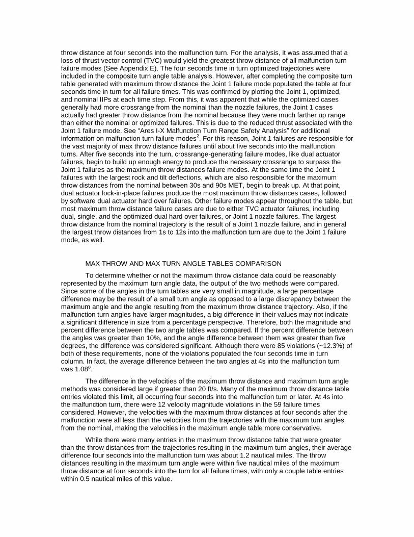
throw distance at four seconds into the malfunction turn. For the analysis, it was assumed that a loss of thrust vector control (TVC) would yield the greatest throw distance of all malfunction turn failure modes (See Appendix E). The four seconds time in turn optimized trajectories were included in the composite turn angle table analysis. However, after completing the composite turn table generated with maximum throw distance the Joint 1 failure mode populated the table at four seconds time in turn for all failure times. This was confirmed by plotting the Joint 1, optimized, and nominal IIPs at each time step. From this, it was apparent that while the optimized cases generally had more crossrange from the nominal than the nozzle failures, the Joint 1 cases actually had greater throw distance from the nominal because they were much farther up range than either the nominal or optimized failures. This is due to the reduced thrust associated with the Joint 1 failure mode. See “Ares I-X Malfunction Turn Range Safety Analysis” for additional information on malfunction turn failure modes

2. For this reason, Joint 1 failures are responsible for

the vast majority of max throw distance failures until about five seconds into the malfunction turns. After five seconds into the turn, crossrange-generating failure modes, like dual actuator failures, begin to build up enough energy to produce the necessary crossrange to surpass the Joint 1 failures as the maximum throw distances failure modes. At the same time the Joint 1 failures with the largest rock and tilt deflections, which are also responsible for the maximum throw distances from the nominal between 30s and 90s MET, begin to break up. At that point, dual actuator lock-in-place failures produce the most maximum throw distances cases, followed by software dual actuator hard over failures. Other failure modes appear throughout the table, but most maximum throw distance failure cases are due to either TVC actuator failures, including dual, single, and the optimized dual hard over failures, or Joint 1 nozzle failures. The largest throw distance from the nominal trajectory is the result of a Joint 1 nozzle failure, and in general the largest throw distances from 1s to 12s into the malfunction turn are due to the Joint 1 failure mode, as well.

MAX THROW AND MAX TURN ANGLE TABLES COMPARISON

To determine whether or not the maximum throw distance data could be reasonably represented by the maximum turn angle data, the output of the two methods were compared. Since some of the angles in the turn tables are very small in magnitude, a large percentage difference may be the result of a small turn angle as opposed to a large discrepancy between the maximum angle and the angle resulting from the maximum throw distance trajectory. Also, if the malfunction turn angles have larger magnitudes, a big difference in their values may not indicate a significant difference in size from a percentage perspective. Therefore, both the magnitude and percent difference between the two angle tables was compared. If the percent difference between the angles was greater than 10%, and the angle difference between them was greater than five degrees, the difference was considered significant. Although there were 85 violations (~12.3%) of both of these requirements, none of the violations populated the four seconds time in turn column. In fact, the average difference between the two angles at 4s into the malfunction turn was 1.08⁰.

The difference in the velocities of the maximum throw distance and maximum turn angle methods was considered large if greater than 20 ft/s. Many of the maximum throw distance table entries violated this limit, all occurring four seconds into the malfunction turn or later. At 4s into the malfunction turn, there were 12 velocity magnitude violations in the 59 failure times considered. However, the velocities with the maximum throw distances at four seconds after the malfunction were all less than the velocities from the trajectories with the maximum turn angles from the nominal, making the velocities in the maximum angle table more conservative.

While there were many entries in the maximum throw distance table that were greater than the throw distances from the trajectories resulting in the maximum turn angles, their average difference four seconds into the malfunction turn was about 1.2 nautical miles. The throw distances resulting in the maximum turn angle were within five nautical miles of the maximum throw distance at four seconds into the turn for all failure times, with only a couple table entries within 0.5 nautical miles of this value.

Even though the two tables were populated using two different methods, the patterns of failure types responsible for both the maximum throw distance and the maximum turn angle were almost identical. As can be seen in Figure 39 and Figure 40 on the following two pages, there are small differences throughout the tables, but the same trends are easily noticed, suggesting that the failures resulting in the maximum throw distance from the nominal trajectory are similar to those causing the maximum turn angle from the nominal.

While the failure types causing the maximum throw distance and angle are very similar, rarely did the same failure cause both characteristics. Many times the two failures causing the maximum throw and angle would be the same type, but with different rock and tilt orientations.

CONCLUSION

Since the 45SW considers only the data from four seconds into the malfunction turn at each time of failure, it appears that the maximum throw distance malfunction data can be reasonably represented by the data from the malfunctions generating the maximum malfunction turn angle. Although there are differences between the composite turn angle table generated with the maximum throw distance and the table populated with the maximum turn angle table delivered in the FFDP, the major discrepancies occur at five seconds into the malfunction turns or later. Four seconds into the malfunction turns, no failure times showed an angle difference greater than five degrees between the maximum turn angle and the malfunction turn angle causing the maximum throw distance from the nominal trajectory. There were some significant differences in the magnitude of the malfunction velocities between the two methods four seconds into the malfunction turn, but the velocities from the maximum turn angle failures were all greater than the velocities caused by the maximum throw distance cases. Therefore, the 45SW was provided with the most conservative malfunction velocity data. Finally, none of the maximum throw distances were more than five nautical miles greater than the throw distances causing the maximum turn angles at four seconds into the malfunction turns.

As the time spent in the malfunction turn increases, the differences in the maximum angle tables and maximum throw tables become significant. However, as long as the 45SW uses only the four seconds time in turn data to create their destruct criteria, there are no concerns with the delivered FFDP composite turn angle table. Through this analysis, the processes to create both the maximum malfunction turn angle tables and the maximum throw distance tables for Ares 1-X have been validated and documented.

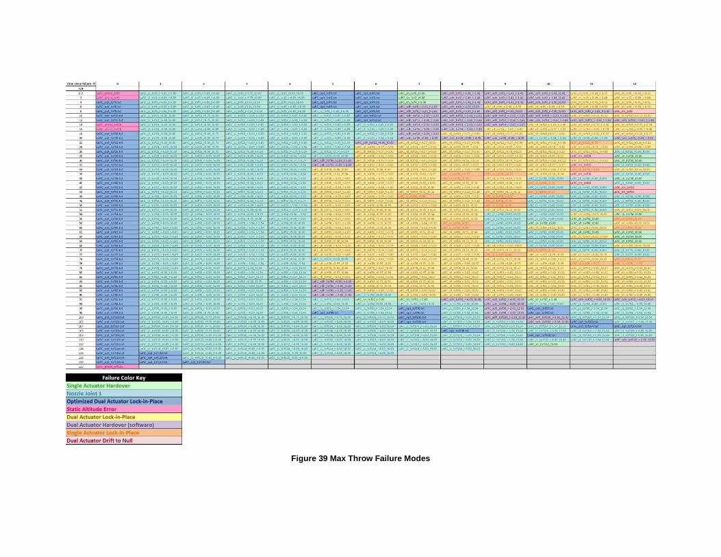
Figure 39 Max Throw Failure Modes

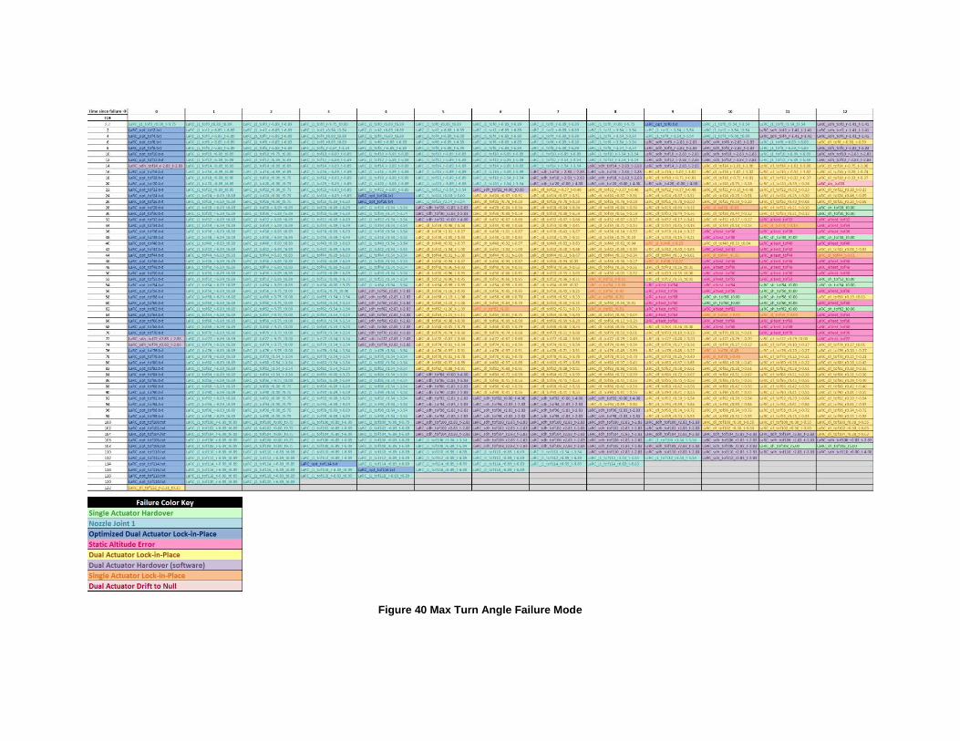
Figure 40 Max Turn Angle Failure Mode