Paleo-Mesoproterozoic Supercontinents – A Paleomagnetic Vie · Paleo-Mesoproterozoic...

Geophysica (2012), 48(1–2), 5–47

Paleo-Mesoproterozoic Supercontinents – A Paleomagnetic View

L.J. Pesonen1*, S. Mertanen2 and T. Veikkolainen1

1 Division of Geophysics and Astronomy, Department of Physics, University of Helsinki, FI-00014 Helsinki, Finland

2 Geological Survey of Finland, FI-02151 Espoo, Finland *Corresponding autor [email protected]

(Received: April 2011; Accepted: October 2011)

Abstract

Various geological and geophysical evidence show that at least two supercontinents, Columbia and Rodinia, existed during the Paleoproterozoic and Mesoproterozoic eras. In this study, updated pa-leomagnetic and isotope age data has been used to define the amalgamation and break-up times of these supercontinents. Before putting the ancient continents to a supercontinent assembly, we have tested the validity of the geocentric axial dipole model (GAD) of the Paleo-Mesoproterozoic geomagnetic field us-ing four methods. The tests yield support to the GAD-model, but do not rule out a ca. 10% non-dipole (octupole) field. In the whole of Proterozoic, Columbia and Rodinia were predominantly in moderate to low paleolatitudes, but during the Paleoproterozoic some parts of Columbia, notably India (Dharwar craton) and Australia (Yilgarn craton), occupied polar latitudes. In the Paleoproterozoic, there were unexpected low-latitude glaciations. The pre-Columbia orogenies were due to a complex set of collisions, rotations and transform or strike slip faultings that caused the orogenic belts to appear obliquely. No prominent difference was observed between paleomagnetically derived and recent geologic models of Columbia. The final amalgamation of Columbia didn’t happen until ca. 1.53 Ga. Columbia broke up at ca. 1.18 Ga during several rifting episodes, followed by a short period of independent drift of most con-tinents. The amalgamation of Rodinia didn’t take place until 1.10 – 1.04 Ga.

Keywords: Supercontinents, Paleoproterozoic, Mesoproterozoic, Columbia, Rodinia, paleomagnetism, paleogeography, mafic dykes, GAD

1. Introduction

The importance of supercontinents in our understanding of the geological evolu-tion of the Earth has been discussed in several articles (e.g., Zhao et al., 2002; Rogers and Santosh, 2004; Li et al., 2008 and references therein). Geological processes linked to the existence of supercontinents include concepts such as large igneous provinces (LIPs) (Ernst and Buchan, 2002), mantle superplume events (Condie et al., 2001), low latitude glaciations and the high obliquity-theory of the rotation axis (Williams and Schmidt, 1997), the "Snowball Earth" hypothesis (e.g., Kirschvink, 1992), carbon iso-tope excursions (e.g., Bekker et al., 2001), fragmentation of continental dyke swarms (Ernst and Buchan, 2001), truncations of tectonic belts and major rifts (Dalziel, 1999), matching of conjugate orogenic belts (e.g., Hoffman, 1991), episodic nature of distribu-tions of magmatic activities (Condie, 1998), discoveries of Precambrian ophiolites (Pel-tonen et al., 1996), and the concept of true polar wander (e.g., Evans, 2003).

Published by the Geophysical Society of Finland, Helsinki

6 L.J. Pesonen, S. Mertanen and T. Veikkolainen

In our previous paper (Pesonen et al., 2003) we assembled the continents into their Proterozoic positions using high quality paleomagnetic data which was available at that time. Since then, not only have new data been published but also novel, challenging geological models of the continental assemblies during the Proterozoic have been pro-posed (e.g., Cordani et al., 2009; Johansson, 2009; Evans, 2009). In this paper, we use the updated palaeomagnetic database (Pesonen and Evans, 2012), combined with new geological information, to define the positions of the continents during Paleoproterozoic (2.5 – 1.5 Ga) and Mesoproterozoic eras (1.5 – 1.04 Ga). We do the reconstructions re-lying mainly on isotopically (U-Pb) dated high quality palaeopoles since this method provides strict information of ancient latitudes of the cratons throughout the Proterozoic time. When compared to the previous database (Pesonen et al., 2003), the new one is both geographically and temporally more abundant and contains 2813 observations al-together.

Although there are recent ideas in establishing the absolute paleolongitudes (see Torsvik et al., 2010), the “longitude - method” is not yet feasible beyond the age of the Gondwana assembly at ca. 500 Ma. Our previous work to construct the Proterozoic po-sitions of continents was limited to twelve time bins based on the availability of data in 2003 (Pesonen et al., 2003). However, at these time slots, some (e.g., 1.88 Ga) of the assemblies were accompanied by only two continents (Laurentia and Baltica) due to lack of reliable data from other continents. In this paper we focus on Paleo-Mesopro-terozoic reconstructions at seven time slots, 2.45 Ga, 1.88 Ga, 1.77 Ga, 1.63 Ga, 1.53 Ga, 1.26 Ga and 1.04 Ga, respectively, but represented by at least four or more conti-nents per each age bin.

Before accepting the reconstructions made by paleomagnetic methods, we had two additional criteria. First, we tested the basic assumption of paleomagnetism, i.e. the validity of the geocentric axial dipole (GAD) hypothesis during the considered age in-terval (Irving, 1964; Meert, 2009). Second, we tested the new reconstructions with cur-rently available geological data. These latter tests include studies of continuations of tectono-magmatic belts from one continent to another, matching conjugate orogenic belts (e.g., Grenvillian belts), searching continuations of dyke swarms, or looking con-tinuations of Proterozoic rapakivi or kimberlite corridors in the assemblies. Some of the continental configurations and the tectonic styles of their amalgamations presented here are in contrast with our previous models (Pesonen et al., 2003). This is mainly due to the addition of newer, more reliable paleomagnetic and/or age data (e.g., the reconst-ruction at 1.53 Ga).

2. Sources of data and used technique

Palinspastic reconstruction of continents relies on the position of continents nuclei (cratons) rather than continents as they exist today. The Archean to Proterozoic conti-nental cores consist of individual cratonic blocks which may have been drifting, accret-ing, colliding and rifting apart again. Therefore, we try to present the cratonic outlines by omitting the post-Proterozoic orogenic or accretional belts (see Pesonen et al., 2003).

Paleo-Mesoproterozoic Supercontinents – A Paleomagnetic View 7

Another feature in concern is the consolidation time of the Precambrian continents. Lau-rentia serves as an example: most of its paleomagnetic poles are derived from rocks within the Superior Province and only a few are derived from other provinces like Sla-ve, Hearne, or the Churchill province (Fig. 1). For post 1.77 Ga, Laurentia was probably already consolidated (Symons et al., 2000; Buchan et al., 2000), since there is an overall agreement of poles from several provinces at this time. However, prior to 1.77 Ga, the situation is more complex. For example, recent paleomagnetic evidences show that in Paleoproterozoic era the Slave craton was located far away (with respect to its present distance) from the Superior craton (Buchan et al., 2009). The same is true for Baltica, where Kola and Karelia cratons may have had their own drifts during Paleoproterozoic even though they are close to each other within present-day Baltica (Mertanen et al. 2001; Pesonen and Sohn, 2009). Therefore, we try to present the cratonic outlines in our reconstructions to better emphasize the actual source blocks of the data. In the follo-wing, and referring to Fig. 1 and Table 1, we use terms such as Laurentia, Baltica etc. for the continents: the reader should, unless otherwise stated, see from Appendix 1 and Table 1 which craton (e.g. Superior, Karelia etc.) is dealed in each case.

Fig. 1. Map showing the continents in their present day geographical positions. Precambrian continental cratons (partly overlain by younger rock sequences) are outlined by yellow shading. The following conti-nents are used in the reconstructions or discussed in text: Laurentia, Baltica, Siberia, North China, India, Australia, Kalahari, Congo, West Africa, Amazonia and São Francisco. In addition, the Precambrian con-tinents not used in present reconstructions, Ukraine, South China, East Antarctica, Dronning Maud Land and Coats Land are shown. The Archean cratons are marked as follows: for Laurentia; Superior (S), Wy-oming (W), Slave (Sl), Rae (R), Hearne (H), for Baltica; Karelia (K); for Australia; North Australia (NA) (Kimberley and Mc Arthur basins), West Australia (WA) (Yilgarn and Pilbara cratons), South Australia (SA) (Gawler craton), for Amazonia; Guyana Shield (G), Central Amazonia (C). Galls projection.


Table 1. Mean values of paleopoles used for reconstructions.

Continent (Craton) refers to text and Fig. 1. N number of entries as shown in Appendix 1. Dr, Ir refer to mean Declination, Inclination of the Characteristic Remanent Magnetization (ChRM) of a central refer-ence location for each continent/craton. Reference locations: Laurentia: 60°N, 275°E, Baltica: 64°N, 28°E, Australia: North Australia NA: 20°S, 135°E, West Australia WA: 27°S 120°E, South Australia SA: 30°S, 135°E, India: 18ºN, 78ºE, Siberia: 60ºN, 105ºE, Kalahari: 25ºS, 25ºE, West Africa: 15ºN, 35ºE, Amazonia: 0°, 295°E, Congo: 5°S, 23°E, São Francisco (São Fr.): 13°S, 315°E, North China: 40°N, 115°E. Plat, Plon are latitude, longitude of the paleomagnetic pole. A95 is the 95% confidence circle of the pole. Greenland poles have been rotated relative to Laurentia using Euler pole of 66.6°N, 240.5°E, rotation angle −12.2° (Roest and Srivistava 1989). S is the mean Angular Standard Deviation as explained in text. Q1-6 is the mean Q (quality factor or grade) of N entries in Appendix 1. E-Plat, E-Plon are the co-ordinates of the single Euler rotation pole, Angle: Euler rotation angle.


The data come mainly from the cratonic areas of the largest continents or conti-nental fragments which are Laurentia, Baltica, Amazonia, Kalahari, Congo, São Fran-cisco, India, Australia, North China, West Africa and Siberia (Fig. 1). The smaller cra-tons or “microcontinents”, such as Rio de la Plata, Madagascar, South China, Taymyr etc. are not included due to lack of reliable data from the investigated period 2.45 – 1.04 Ga. Neither included in the current analysis are the large Saharan craton in Africa, sev-eral small South American (e.g., Pampia, Paraná), Indian (Eastern Ghats), East Antarc-tican (Mawson, Rayner, Wilkes), and East European (Volgo-Uralia) cratons or micro-continents, since no realiable Paleo-Mesoproterozoic paleomagnetic data are so far available from them (see Li et al, 2008, and references therein). Some cratons, which are now attached with another continent than their inferred original source continent, have been rotated back into their original positions before paleomagnetic reconstruction. For example, the Congo craton will be treated together with the São Francisco craton, since geological and paleomagnetic data are consistent that they were united already at least since 2.1 Ga (e.g., D´Agrella-Filho et al., 1996). The rotations were done assuming that their fragmentation took place in the breakup of Gondwanaland and therefore they are treated in their traditional Gondwana configuration. Similarly, Greenland is treated in its pre-Mesozoic fit with North America using the Roest and Srivastava (1989) model of their separation.

3. Data selection

The data came from the updated Precambrian paleomagnetic compilation done at the University of Helsinki and at Yale University (Pesonen and Evans, 2012). Every entry has been coded to its source continent/craton and also rated according to grading scheme by Van der Voo (1990) with seven steps (Q1-7). We used six out of seven grades since the last grade (Q7) cannot be applied meaningfully to Precambrian data. In gen-eral, we accepted data with total Q higher or equal to 4. However, occasionally we ac-cepted entries with a smaller Q if there are reasons for this, such us new ages or new pa-leomagnetic information. The used data are compiled in Appendix 1.

A Fisher mean (Fisher, 1953) was calculated when multiple poles (value N in Ta-ble 1) for a particular craton and a particular bin were available (Appendix 1). The ad-vantage of this technique is that the mean pole is obtained with enhanced accuracy but not always with better precision (the A95 value between poles ís sometimes higher than those of individual poles).

4. Basic tests

Before making a continental reconstruction using Table 1 data, we must be as-sured that the basic assumptions of paleomagnetism are fulfilled. These assumptions are that: (i) the geomagnetic field during the Paleo-Mesoproterozoic is that due to geocentric ax-ial dipole (GAD-hypothesis; Irving, 1964; see also Meert, 2009).


(ii) the Earth was spherical and its radius has not changed markedly during the time span involved (Schmidt and Williams, 1995). (iii) the inclination variations in data of various ages represent continental drift and not true polar wander (TPW) (Evans, 2003).

While the two latter assumptions can be at least in most cases neglected (see Ev-ans and Pisarevsky, 2008 and references therein), the first one requires some discussion (see Kent and Smethurst, 1998; Meert et al. 2003; Tauxe and Kodama, 2009).

The best way to test the GAD-model during the Precambrian times uses the incli-nation frequency analysis of Evans (1976). This method is based on the fact that the ax-ial (zonal) spherical harmonic coefficients have characteristic inclination distribution when averaged over the spherical Earth (Evans, 1976). For example, the Gauss coeffi-cient of the geocentric axial dipole (g1

0) has very different inclination distribution than the axial guadrupole (g2

0) or octupole (g30) components. The method can be applied to

Precambrian era provided that the continents, during their course of drifting, have pa-leomagnetically “sampled” all latitudes in equal amounts of time. This motion is diffi-cult to prove and leaves a caveat for this method (see discussions in Meert et al., 2003; McFadden, 2004; Evans and Hoye, 2007). Unfortunately, the very low amount of data in Table 1 (42 entries) does not allow the GAD-model to be tested properly by the incli-nation data of Table 1 since the required minimum amount of globally distributed data for the analysis is about 300, when 9 latitudinal bins are applied for each of the 23 cra-tons. The minimum is determined by the limitations of chi-square testing (Veikkolainen, 2010). However, if we take inclination values from igneous rocks of all continents from the database of Pesonen and Evans (2012) of the interval of 2.45 – 1.04 Ga with quality factor Q > 2, we get 645 entries to the analysis. These data yield a best fit model (Fig. 2) where the quadrupole content (relative to GAD) is zero while the octupole content is 11%. Although the distributions are still biased to shallower inclinations (Figure 2), the

Fig. 2. Frequency distribution of inclinations during 2473-1020 Ma. Global data base of Pesonen and Ev-ans (2012), only igneous rocks with Q > 2. Green: observed distribution, Red: best fit with g1º = -30 000

nT, G2 (= g2º/ g1º) = O % and G3 (= g3º/ g1º) = 11% . Blue: GAD-curve.


new data are much closer to GAD than in any previous analysis (Kent and Smethurst, 1998). It is possible that the small bias towards low inclinations is caused by a small permanent (~10%) octupole component prevailing during the Paleo-Mesoproterozoic era. But more likely this bias is caused by the fact that the continents may not have sampled the Earth´s surface completely (Meert et al. 2003; McFadden, 2004; Meert, 2009) or that the Proterozoic supercontinents simply had a tendency to occupy near equatorial latitudes for long times due to dynamic reasons (Evans, 2003 and references therein).

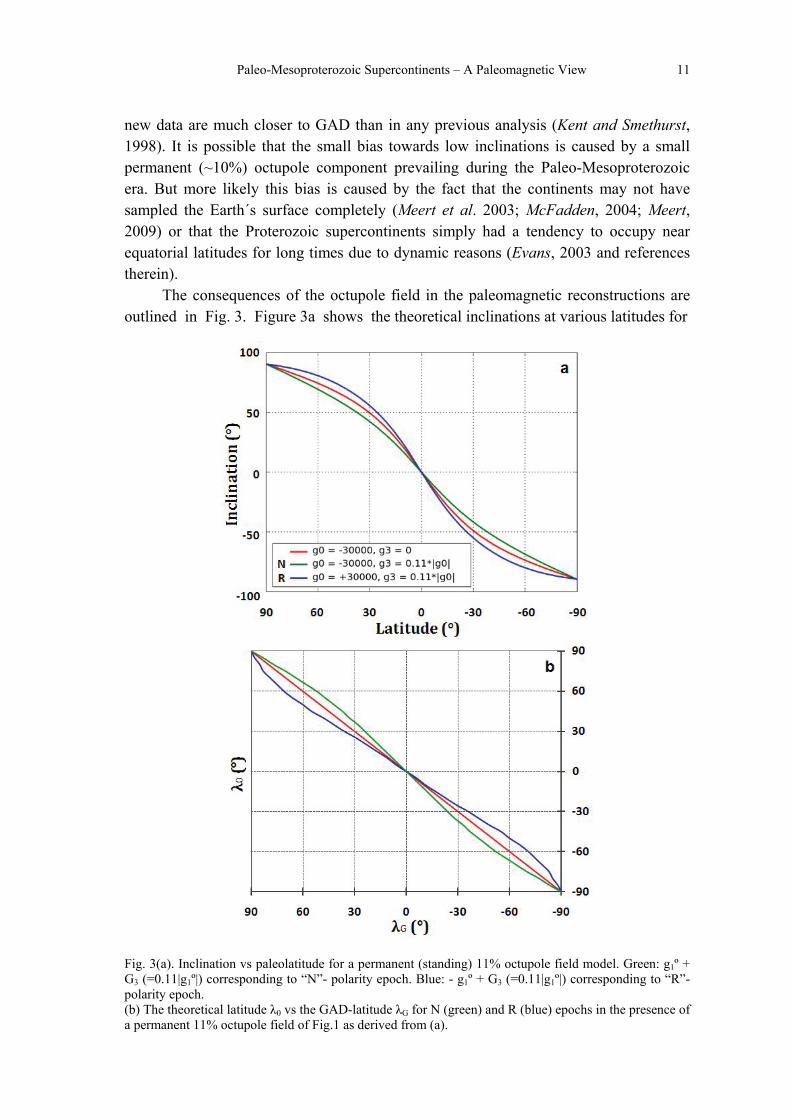
The consequences of the octupole field in the paleomagnetic reconstructions are outlined in Fig. 3. Figure 3a shows the theoretical inclinations at various latitudes for

Fig. 3(a). Inclination vs paleolatitude for a permanent (standing) 11% octupole field model. Green: g1º + G3 (=0.11|g1º|) corresponding to “N”- polarity epoch. Blue: - g1º + G3 (=0.11|g1º|) corresponding to “R”-polarity epoch. (b) The theoretical latitude λ0 vs the GAD-latitude λG for N (green) and R (blue) epochs in the presence of a permanent 11% octupole field of Fig.1 as derived from (a).


the two polarities (N, R) in the case when GAD changes polarity while the 11% octu-pole field remains constant. We can see that in the northern hemisphere, the R-polarity inclinations are enhanced from the GAD-values, whereas the N-polarity inclinations are lowered. In the southern hemisphere, the situation is opposite. Fig. 3b shows the depar-tures of the observed paleolatitude from the GAD-value for the two polarities in the case of the permanent 11% octupole field. We see that largest departures are of the order of ~10° and occur at middle latitudes. Near the poles, and especially at shallow latitudes, the field is closer to GAD-field (see also Schmidt, 2001).

Figure 4 shows the observed inclination asymmetry (ΔI) between N and R polar-ity epochs during Paleo-Mesoproterozoic, in cases where dual polarity paleomagnetic

Fig. 4(a). Inclination asymmetry |∆I| vs age (see also Schmidt, 2001). (b) Inclination asymmetry (|∆I|) vs paleolatitude | λ | of global data (2473-1020 Ma). Only igneous rocks with Q > 2.


results are available (see Pesonen and Nevanlinna, 1981). Only inclination asymmetries can be used since the declination asymmetry, in case of zonal geomagnetic field, is zero. The results (Fig. 4a) reveal generally low to moderate ∆I (average ~15°) during 2.45 – 1.04 Ga (see also Schmidt, 2001). No correlation of ∆I with paleolatitude is observed (Fig. 4b). We interpret the lack of large inclination asymmetries to point towards a GAD-dominated field consistent with the inclination frequency analysis. Again, the possibility for a 10% octupole field contamination cannot be ruled out.

Figure 5 shows the result of the paleosecular variation (PSV) test. Here we com-pare the curve of the angular standard deviation (S) of the poles vs paleolatitude during 2.45 – 1.04 Ga with the GAD-curve (i.e, Model G of Merrill et al. 1996). The data are the same as used in inclination analysis. The result reveals that the observed S-values appear (notably towards the pole) to be above the GAD-curve. This can be simply due to lack of within-site correction in the calculated S-values (which is typically of the or-der of ≤2°; Irving, 1964) or it may reflect the previously discussed 11 % octupole con-tamination in the geomagnetic field during Paleo-Mesoproterozoic era.

Fig. 5. Paleosecular Variation (PSV) of global data for age 2473 – 1020 Ma. Only igneous rocks (N=796) with Q > 2. S Angular Standard Deviation (Merrill et al., 1996), |λ| absolute value of paleolatitude. Data calculated as means for 10 degrees latitude bins. Numbers show amount of data in each bin. The error bars in S and λ are ± one standard error of the mean. The solid curve is the GAD-curve (= model G of Merrill et al. (1996)). The last point (at bin 80-90 deg) has a great uncertainty due to low amount of data. See text.

The fourth model to test the validity of GAD calls for the internal consistency of the poles of the same age but derived from sampling areas which are located at far dis-tance from each other within the same craton. This test has been thoroughly discussed in Pesonen et al. (1989) and Evans and Pisarevsky (2008). They concluded that the avail-able data (e.g. the 1.88 – 1.87 Ga Svecofennian gabbro poles of Baltica, the 1.27 – 1.25 Ga post-Jotnian dolerite poles of Baltica, and the 1.26 Ga Mackenzie dyke poles of Laurentia) support the GAD model within the error limits.


In summary, although we cannot be sure, that the field during the Paleo-Mesoproterozoic era was a pure GAD-field, it serves as a good proxy for our paleomag-netic reconstructions. The possible departures from the GAD, caused by the ~10% octu-pole field, can produce minor errors to our reconstructions at middle latitudes as will be discussed later (see also Schmidt, 2001; Van der Voo and Torsvik, 2001).

4.1. Euler-rotations

In making the reconstructions we used the ”two-step” Euler-rotation method used in Pesonen et al. (2003). The cratons were first moved onto their ancient latitudinal po-sitions and orientations by applying the first rotation around an Euler-pole located at the equator. The continents were then rotated around a second Euler-pole, located at the present geographic North Pole. This latter rotation moves the continent along a constant latitude circle. The amount of latitudinal shift of the continent depended on how close to the neighbouring continent it was allowed to move, which depends on geological con-straints. The two Euler-pole rotations were then combined to give a single Euler pole and rotation angle, which places the continent onto the location shown in the reconstruc-tions. Table 1 gives the co-ordinates of the single Euler poles and rotation angles for all reconstructions.

As described in Pesonen et al. (2003), the hemispherical ambiquity due to unde-fined polarity in pre-Phanerozoic times must also be considered by looking both north-ern and southern hemisphere options for each continent. In final tuning of cratons into the reconstructions (Fig. 6–12), we used geological piercing points, such as orogenic or accretional belts, mafic dyke swarms, kimberlite occurrences, rapakivi massifs, ophio-lites, and lithostratigraphic data (Pesonen et al., 2003). In addition to these geological piercing points, we used the following palaeomagnetic criteria in validating the recon-structions:

(i) The magnetic polarity had to be the same from one continent to another during the life time of the assembly. Since we do not know the "absolute" polarity during Paleo-Mesoproterozoic, we seeked distinct polarity patterns (e.g., long single polarity inter-vals) from one continent to another (e.g., Pesonen and Neuvonen, 1981; Buchan et al., 2000).

(ii) The drift rates of the cratons had to be comparable during the lifetime of the assem-bly. The rates should not have exceeded markedly the Cenozoic rates (e.g., Meert et al., 1993).

If a geologically and paleomagnetically sound configuration of the continents (cratons) were found, we kept them together to indicate that they were part of a super-continent. If we did not find an acceptable geological continuation or matching, we kept the cratons apart from the assembly.


5. Age bins

Seven age bins were chosen for reconstructions in this work and they are 2.45, 1.88, 1.78, 1.63, 1.53, 1.26 and 1.04 Ga, respectively. The poles, their ages and other relevant data are listed in Appendix 1 and the mean paleopole data in Table 1. The cor-responding reconstructions are shown in Figs. 6-12. Apart from possible deviations from the GAD-model, the main error arises from the uncertainty in the pole position as expressed by the 95% confidence circles (A95) of the mean poles.

6. Continental reconstructions during the Paleoproterozoic

6.1 Reconstruction at 2.45 Ga

Meert (2002), in his Columbia reconstruction, divided the pre-Proterozoic cratons into three ancient continents, Atlantica, Ur and Nena reflecting their derivation from three but separate Archean land masses. The cratons Amazonia, Guyana, Congo, São Francisco and West Africa are fragments of Atlantica. Australia, India, Antarctica, Madagaskar and Kalahari are pieces of the ancient continent Ur and Laurentia, Siberia, Baltica and North China are derived from the ancient Nena-continent. The existence of these ancient land masses are tested in the following reconstructions.

Table 1 summarizes the data used for reconstruction at 2.45 Ga (Fig. 6). Results are available from two Nena fragments (Laurentia and Baltica) and from two Ur frag-ments (Australia and India). Interestingly, the Superior craton from Laurentia and the Karelia craton from Baltica lie near the equator whereas the Ur fragments, Yilgarn from Australia and especially Dharwar from India, are at high, almost polar (south) latitudes. Thus, the split of the Archean supercontinent Kenorland (Pesonen et al., 2003) into Nena and Atlantica land masses holds during the early Paleoproterozoic.

Previously, Pesonen et al. (2003), used the so called D-component of remanent magnetization (a SE down pointing remanence direction) in Baltica as a primary 2.45 Ga magnetization, documented in many 2.45 Ga intrusions in Kola and Karelia cratons (e.g. Mertanen et al., 2006b). This interpretation does not support the “Superia” super-craton model (Superior-Karelia-Wyoming unity) of Bleeker and Ernst (2006) at 2.45 Ga, since the D-magnetization places Karelian craton of Baltica some 30 degrees south of Superior province (Mertanen et al., 2006b; Salminen et al., 2010). It is however, pos-sible that the D-magnetization is actually slightly younger, ca. 2.40 Ga, obtained during cooling of the Karelian craton after the widespread magmatic heating of the crust by the 2.45 Ga intrusions (Mertanen et al., 1999). Instead, if we accept that the south-shallow D´-component of remanent magnetization, found at baked contact zones of the 2.45 Ga intrusions in Karelia (Mertanen et al., 1999), is the primary 2.45 Ga remanence, we end up to reconstruction shown in Fig. 6. In this model the Matachewan (Superior province) (Evans and Halls, 2010) and the Karelian (Mertanen et al, 1999) dyke swarms become parallel, and fairly close to each other, pointing to a plume in the center of the “Superia” supercraton, as suggested by Bleeker and Ernst (2006).


Dykes of ~2.45 – 2.37 Ga ages exist also in Australia (Yilgarn) and India (Dhar-war), as shown in the reconstruction of Fig. 6, which is mainly the same as proposed by Halls et al. (2007), albeit that the used projections differ. The Widgiemooltha swarm (~2.42 Ga; Evans, 1968) of the Yilgarn craton has a similar trend as the Matachewan-Karelia swarms in this assembly, but its distance to these swarms is more than 90o in latitude (>10,000 km), which does not support a genetic relationship between Yilgarn and Superior-Karelia unity at 2.45 Ga. On the other hand, the E-W trending dykes of the Dharwar craton, with an age of 2.37 Ga (Halls et al., 2007; French and Heaman, 2010), form a continuation with the Widgiemooltha swarm (Fig. 6). The Widgiemooltha and Dharwar dykes can possibly be associated with another mantle plume in the southern hemisphere.

Fig. 6. Reconstruction of Archean cratons at 2.45 Ga. Data available from Laurentia (L), Baltica (B), Australia (A) and India (I) (Table 1). The cratons Superior (Laurentia), Karelia (Baltica), West Australia (Yilgarn) and Dharwar (India) are shown in grey shading. Dyke swarms are shown as red sticks and they are: Matachewan dykes (Laurentia), Russian-Karelian dykes (Baltica), Widgiemooltha dykes (Yilgarn) and Dharwar E-W dykes (India). Orthogonal projection.

Between 2.40 Ga and 2.22 Ga the Superior, Karelia and Kalahari cratons experi-enced one to three successive glaciations (Marmo and Ojakangas, 1984; Bekker et al., 2001). It is noteworthy that the glaciogenic sequences also contain paleoweathering zones, lying generally on top of the glaciogenic sequences. These early Paleoprotero-zoic supracrustal strata are similar to Neoproterozoic strata that also contain glaciogenic sequences and palaeoweathering zones (e.g., Evans, 2000). Moreover, in both cases the palaeomagnetic data point to low paleolatitudes (≤ 45 degrees) during glaciations. Tak-ing Laurentia as an example, it maintained a low latitude position from 2.45 Ga to 2.00 Ga during the time when the glaciations took place (e.g., Schmidt and Williams, 1995). For the other continents we do not have reliable palaeomagnetic data to show their lati-tudinal positions during the early Paleoproterozoic glaciations. Tentatively, Karelia ap-


pears to have been at low to intermediate latitudes during 2.45 – 2.15 Ga (Neuvonen et al., 1997; Mertanen et al., 2006b; Salminen et al., 2010). Furthermore, if the Superia model of Bleeker and Ernst (2006), suggesting unity of the Karelia and Superior cratons during the whole time period from 2.45 Ga to 2.1 Ga, is valid, it places Karelia at sub-tropical paleolatitudes of 15–45° at that time (Bindeman et al., 2010).

At least four models have been presented to explain the low latitude glaciations: (i) the “Snowball Earth” hypothesis, (ii) the concept of a large Earth’s obliquity, (iii) the remagnetisation explanation, and (iv) the non-dipole model of the geomagnetic field. Models (i) – (iii) are thoroughly discussed in literature (see Pesonen et al. 2003 and ref-erences therein). Model (iv) has been tested in this work with a result that a ~10% octu-pole field can cause a 10° error in paleolatitudes for continents occupying middle lati-tudes. This is not sufficient to “move” continent from high latitudes (where glaciatons take place) to near equatorial latitudes.


The period of 1.90 – 1.80 Ga is well known in global geology as widespread oro-genic activity. Large amounts of juvenile crust were added to the continental margins, and black shales, banded iron formations (BIFs), evaporites and shallow marine phos-phates were deposited in warm climatic conditions (Condie et al., 2001). These deposits support the existence of a supercontinent (“Early Columbia”) or at least a huge land-mass at low to moderate latitudes at ca. 1.88 Ga (see Pesonen et al., 2003 and references therein).

Table 1 shows that for 1.88 Ga, reliable poles are available from three Nena areas (Baltica, Laurentia and Siberia), from two Ur cratons (Australia and Kalahari), and from one Atlantica craton (Amazonia). The reconstruction is shown in Fig. 7. All continents in Fig. 7 have moderate to low latitudinal positions. The assembly of Laurentia and Bal-tica at 1.88 Ga, together with Australia and Siberia marks the onset time of development of the supercontinent Columbia although the final amalgamation occured as late as ~1.53 Ga (see Chapter 6.5). The position of Baltica against Laurentia is rather well es-tablished as paleomagnetic data are available from several Svecofennian 1.88 – 1.87 Ga gabbros. However, the age of the mean pole is somewhat uncertain since the magnetisa-tion ages of the slowly cooled gabbro-diorite plutons may be 10 – 20 Ma younger than their crystallization age (Mertanen and Pesonen, 2005). In addition, the position of Laurentia is somewhat uncertain due to problems related to the “B” pole of the Molson dykes (Halls and Heaman, 2000). We note that the Laurentia-Baltica unity in Fig. 7 de-parts from the 2.45 Ga configuration (Fig. 6), consistent with separation of Superior from Karelia between 2.45 Ga and 2.05 Ga (Bleeker and Ernst, 2006). The data further suggest that a considerable latitudinal drift from 2.45 Ga to 1.88 Ga took place for Laurentia but much less for Baltica.


Fig. 7. Reconstruction of cratons and orogenic belts (green) at 1.88 Ga. The Archean cratons are shown in gray. Data available from Laurentia (L), Baltica (B), Amazonia (Am), Siberia (S), Australia (A) and Ka-lahari (K). The ca. 1.90 - 1.80 Ga orogenic belts are shown in dark green and they are: Laurentia: Nagssugtoqidian (N), Ketilidian (K), Torngat (T), Trans-Hudson (TH), Penokean (P), Woopmay (W), Taltson-Thelon (T-T), Baltica: Lapland-Kola (L-K), Svecofennian (Sv), Amazonia: Ventuari-Tapajos (V-T), Siberia: Akitkan (A), Australia: Capricorn (C), Kalahari: Limpopo (L). For explanation, see text.

The model in Fig. 7 provides the following scenario to explain the ca. 1.90 – 1.80 Ga orogenic belts in Laurentia and Baltica. After rifting at ~2.10 Ga, both continents drifted independently until ~ 1.93 Ga. Subsequently, the Superior craton collided with Karelian craton causing the Nagssugtoqidian and Torngat orogens in Laurentia and the Lapland -Kola orogen in Baltica. It is likely that collisions between Superior and Kare-lia (or consolidated continents Laurentia and Baltica), caused intra-orogenic belts be-tween Superior and Slave craton in Laurentia and between Kola and Karelia cratons in Baltica. Simultaneously, in Baltica, accretion and collision of several microcontinents to the margin of the Karelian craton may have taken place (Lahtinen et al., 2005). The complexity of the collisions of the Archean cratons and accretions to the craton margins is manifested by the anastomosing network of 1.93–1.88 Ga orogenic belts in Baltica and Laurentia (Fig. 7). The same seems to have happened in other continents, too, like in Australia, Kalahari, and Amazonia. Buchan et al. (2000) discusses in more detail how the patterns of these orogenic belts were formed during the collisions, including rota-tions and strike slip and transform faultings.

In addition to the above mentioned collisions within Baltica and Laurentia, a col-lision of Laurentia-Baltica with a “third continent” may be responsible for at least some of the 1.93 – 1.88 Ga orogenic belts (Pesonen et al., 2003). Candidates for this 'third continent' include Amazonia, North China, Australia, Siberia and Kalahari. Each of these have 1.93 – 1.88 Ga orogenic belts: the Trans China orogen in China, the Capri-corn orogen in Australia, the Ventuari-Tapajos orogen in Amazonia, the Akitkan orogen is Siberia and the Limpopo belt in Kalahari (Geraldes et al., 2001; Wilde et al., 2002).


Although the data from Amazonia are not of the best quality (Q ≈ 2-3), Amazonia was probably not yet a part of the 1.88 Ga Laurentia-Baltica assembly (Fig. 7).

Based on new ~1.88 Ga paleomagnetic data of dykes from the Bastar craton, In-dia, Meert et al. (2011) have presented a novel, paleomagnetically constrained model of Columbia at 1.88 Ga. Although our model of Columbia (Fig. 7) lacks India, it is strik-ingly similar to the model of Meert et al. (2011). In contrast, our model and that by Meert et al. (2011) differ from the geologically made Columbia by Zhao et al. (2004). As pointed out by Meert et al. (2011), the differences can be due to the fact that Colum-bia was yet in its amalgamation stage at 1.88 Ga, a conclusion supported also by data of this paper.


Reliable palaeomagnetic data at 1.78 Ga come from Laurentia, Baltica, North China, Amazonia, Australia, India and Kalahari (Fig. 8). The 1.78 Ga “Early Columbia” is made of two landmasses: the first one consists of an elongated large continental area of Laurentia, Baltica, North China and Amazonia, and the second one contains Austral-ia, India and Kalahari. These continents remained at low to intermediate latitudes during 1.88 – 1.77 Ga. The used poles are listed in Appendix 1 and Table 1. The 1.78 Ga con-figurations of Baltica and Laurentia differ from that at 1.88 Ga. This difference is mostly due to rotation of Laurentia relative to Baltica which stayed more stationary. The considerable rotation of Laurentia may be incorrect and result of poor palaeomagnetic data, but it is also possible that there was a long-lasting accretion to the western margin of the closely situated Laurentia-Baltica cratons. This was not a simple accretional growth event but included relative rotations along transform faults between the accret-ing blocks (Nironen, 1997) until their final amalgamation at ca. 1.83 Ga. It is also pos-sible that the docking of Ukraine with Baltica at ~1.78 Ga (see Bogdanova, 2001) trig-gered minor block rotations within Baltica. Support for the continuation of Laurentia-Baltica from 1.83 Ga to 1.78 Ga (and even to 1.12 Ga; see Salminen et al., 2009) comes from the observations that the geologically similar Trans Scandinavian Igneous Belt (TIB) I-belt in Baltica and the Yavapai/Ketilidian belts of Laurentia (e.g., Karlstrom et al., 2001; Åhäll and Larson, 2000) become laterally contiguous when reconstructed ac-cording to palaeomagnetic data of the age of 1.83, 1.78 Ga and 1.25 Ga (Buchan et al., 2000; Pesonen et al., 2003).

Several reconstructions models have been proposed for the onset of Columbia at ca. 1.78 Ga (see e.g. Meert, 2002; Bispo-Santos et al., 2008; Kusky et al., 2007 and ref-erences therein). The 1.78 Ga Columbia model (Fig. 8) of this work is similar to the model by Bispo-Santos et al. (2008).

Wilde et al. (2002) have proposed a model of North China - Baltica connection where North China is placed north of Baltica. Their geological rationale was to seek connections of the 1.9 – 1.8 Ga Kola-Karelian and the coeval Trans-North China orogens so that Karelia craton of Baltica may be contiguous with the western block of North China craton and the Kola craton being contiguous with Eastern Block of the


North China craton. No paleomagnetic data are available from the 1.9 – 1.8 Ga rocks of North China craton to test this model, but the paleomagnetically made configuration at 1.78 Ga (Fig. 8) does not support the model by Wilde et al. (2004), unless North China has rapidly drifted from north of Baltica (at ~1.9 – 1.8 Ga) to south of Baltica at 1.78 Ga (Fig. 8).

Fig. 8. The reconstruction of continents at 1.78 Ga. Data available from Laurentia (L), Baltica (B), North China (NC), Amazonia (Am), India (I), Australia (A) and Kalahari (K). The Archean cratons are shown as grey shading (see Figs. 1 and 6-7). The 1.90-1.80 Ga orogenic belts (green) in Laurentia, Baltica, Aus-tralia, Amazonia and Kalahari are the same as in Fig. 7. In North China: Trans-North China orogen (T-N); India: Central Indian tectonic zone (C-I). The ca. 1.8–1.5 Ga orogenic belts (black): Laurentia: Ya-vapai (Y), Baltica: Transscandinavian Igneous Belt (TIB), Amazonia: Rio Negro-Juruena (R-N); Austral-ia: Arunta (Ar). The 1.78–1.70 Ga rapakivi granites are shown as red circles.

It is likely that Australia and India, in this early Columbia positions (Fig. 8), are on their way to dock later with Laurentia and Baltica. Idnurm and Giddings (1995) show a reconstruction between Australia and Laurentia during 1.70 – 1.60 Ga ago, which differs from our model. Their model places Australia close to the so called SWEAT (South West US and East Antartica connection; Moores, 1991) configuration, whereas our data suggest that Australia is neither compatible with the SWEAT nor with the AUSWUS (Australia and South West US connection; Burrett and Berry, 2000) con-figuration. Karlström et al. (2001) stress that geological data of the 1.80 – 1.40 Ga belts from Laurentia-Baltica landmass (such as Yavapai, Labradorian-Ketilidian and TIB belts) continue into Arunta belt of eastern Australia. This is palaeomagnetically possi-ble: if we allow ±15° freedom in paleolatitude and some 30° anticlockwise rotation of Australia in Fig. 8 (due to pole error of 18.3° (Table 1) or due to 11% octupole field), we are close to Karlström et al. (2001) assembly of Baltica-Laurentia-Australia at 1.78 Ga. In this work, at 1.78 Ga, we keep Australia slightly apart from Laurentia to let it be together with its “Ur partner” India.


The palaeomagnetic data from Amazonia at 1.78 Ga shows that it was located in southern hemisphere. The occurrence of 2.0 – 1.8 Ga Ventuari-Tapajos orogenic belt and the successfully rejuvenating 1.8 – 1.5 Ga Rio Negro Juruena belt in Amazonia with the roughly coeval Svecofennian orogenic belts in Baltica (1.9 – 1.5 Ga) (Figs. 8–9) lead us previously to propose that these belts are conjugate collisional belts. It is possi-ble that these belts represent the earliest phases of a longterm accretional orogeny (see discussion in Pesonen et al. (2003) and Pesonen and Sohn (2008). We return to this in the next reconstruction (Chapter 6.4).

Several episodes of rapakivi magmatism are known during the Paleo-Mesoproterozoic (e.g., Rämö and Haapala, 1995; Dall´Agnoll et al., 1999; Vigneresse, 2005). The 1.77 – 1.70 Ga and the slightly younger 1.75 – 1.70 Ga rapakivi-anorthosites are known in Laurentia, Ukraine (part of Baltica), North China and Amazonia (Fig. 8). Due to their sparse occurrence they cannot be used to test the reconstruction at 1.78 Ga.

Fig. 9. The reconstruction of continents at 1.63 Ga. Data available from Laurentia (L), Baltica (B), Ama-zonia (Am), Australia (A) and Kalahari (K). The 1.8–1.5 Ga orogenic belts (black) are: Laurentia: Ya-vapai-Mazatzal (Y-M), Labradorian (L), Ketilidian (K), Baltica: Gothian (G), Transscandinavian Igneous Belt (TIB), Amazonia: Rio Negro-Juruena (R-N), Australia: Arunta (Ar). For other belts, see Figs. 7-8. The dotted position of Amazonia shows the paleomagnetic position if Table 1 data are taken as face val-ues whereas the suggested position of Amazonia, south of Baltica, is favoured geologically, and is within paleomagnetic error bars (see text). The SE pointing arrow shows the direction of movement for Amazo-nia. The 1.63 Ga rapakivi intrusions and related dykes are shown as red circles and sticks, respectively. For explanation, see text.


The late Svecofennian orogenic belts in Baltica, which are progressively younging towards SW, such as the TIB 1 and 2 belts, the Gothian belt and the corresponding belts in Laurentia (Labradorian, Yavapai-Mazatzal) and in Amazonia (Rio Negro Juruena) are all produced by successive accretions from west onto the cratonic margins. Thus,


accordingly, Amazonia can be continuos rather than conjugate with Baltica-Laurentia assembly. Current geological thinking (e.g., Åhäll and Larson, 2000; Geraldes et al., 2001, and references therein) also favour the idea that all these coeval belts in Laurentia, Baltica and Amazonia are accretional and all formed during Cordilleran type subduction and arc-accretion from west to a convergent margin.

For the 1.63 Ga reconstruction, palaeomagnetic data are available from Laurentia, Baltica, Amazonia, Australia and Kalahari (Fig. 9, Table 1). Using the data in Table 1 as face values places Amazonia onto the same latitude as Baltica and into a situation where the successively younging orogenic belts in Baltica have a westerly trend in the same sense as in Amazonia (Fig. 9). In Pesonen et al. (2003) Amazonia was shifted some 25 degrees southeast which is possible within maximum errors of used poles. This configu-ration, shown as lighter colour in Fig. 9, is a continuation of the previously proposed “elongated” Laurentia-Baltica-Amazonia assembly. In this configuration, the successive orogenic belts show a westward younging trend in all three continents (e.g., Åhäll and Larson, 2000; Geraldes et al., 2001). Although geological evidences strongly support the continuation of Laurentia-Baltica-Amazonia landmass, there is still the possibility that final docking of Amazonia took place later than 1.63 Ga.


Reliable palaeomagnetic data at 1.53 Ga come from Laurentia, Baltica, Amazonia, Australia, North China and Siberia (Fig. 10a). The assembly of Laurentia-Baltica at 1.53 Ga differs only slightly from the 1.78 – 1.63 Ga configurations. Therefore, taking into account the uncertainties in the poles, we believe that the previously proposed Lauren-tia-Baltica unity (where Baltica is along the eastern margin of Greenland, Figs. 8-9) holds still at 1.53 Ga (see also Salminen and Pesonen, 2007; Lubnina et al., 2010).

Recently, Johansson (2009) has proposed a novel configuration of Columbia called SAMBA-assembly, including Laurentia, Baltica, Amazonia and West Africa at ~1.5 Ga (Fig. 10b). The assembly is based on geological continuations without using paleomagnetic data. In this assembly, Baltica is in the center, Laurentia on its NW side, Amazonia is towards south and West Africa towards SE of Baltica, respectively. In SAMBA, the three continents, Laurentia, Baltica and Amazonia form a bumerang-type elongated large continent.

Our paleomagnetic reconstruction (Fig. 10a) is rather similar to SAMBA (West Africa is omitted in lack of reliable data). However, as seen in 1.88 Ga, 1.78 Ga and 1.63 Ga reconstructions (Figs. 7–9), Baltica is located so that the Kola peninsula is ad-jacent to present southwestern Greenland while in the SAMBA reconstruction Baltica is rotated ca. 90 degrees with respect to Laurentia. It shall be noted that while our image (Fig. 10a) is plotted onto a spherical projection, the image (Fig. 10b) of Johansson (2009) is not, and therefore some of the discrepances may be only apparent due to dif-ferent projections. We can see that in both models successively younging orogenic belts from 1.88 Ga to ~1.3 Ga in all three continents show continuations as described in pre-vious Chapters.


Fig. 10. (a) Paleomagnetic reconstruction of supercontinent Columbia at 1.53 Ga. Data available from Laurentia (L), Baltica (B), Amazonia (Am), Siberia (S), Australia (A) and North China (NC). The ca. 1.55-1.50 Ga rapakivi intrusions and related dykes are shown as red circles and sticks, respectively. (b) Geologically made reconstruction of the ca. 1.8–1.3 Ga “SAMBA” consisting of Laurentia-Baltica-Amazonia as modified after Johansson (2009) without West-Africa. For explanation, see Figs. 7–9.

One of the major peaks of rapakivi-anorthosite pulses took place during 1.58 – 1.53 Ga (Rämö and Haapala, 1995; Vigneresse, 2005). The coeval occurrences of bi-modal rapakivi granites and anorthosites associated with mafic dyke swarms in Baltica and Amazonia during 1.58 – 1.53 Ga further supports the close connection between these continents in the Columbia/SAMBA configuration (Johansson, 2009; Pesonen and Sohn, 2009). This rapakivi activity could be consistent with a hot spot underlying the Baltica-Amazonia-Australia landmass (Pesonen et al., 1989). Another possibility is that the coeval rapakivi-anorthosite magmatism is a distal response in the foreland for the prolonged accretions that took place in the continental margin of Baltica-Amazonia as described previously (Åhäll and Larson, 2000).

The position of Australia in Fig. 10a on the present western coast of Laurentia is roughly halfway between the SWEAT and AUSWUS configurations (Karlström et al., 2001). The palaeomagnetic data thus suggests that Australia was also part of Columbia (and SAMBA). The occurrence of ca. 1.60 – 1.50 Ga rapakivi intrusions in Australia further support the idea that Australia was in close connection with Laurentia-Baltica-Amazonia at 1.53 Ga.

Palaeomagnetic data could allow Siberia to be in contact with present northern Laurentia at 1.53 Ga (Fig. 10a). However, Pisarevsky and Natapov (2003) have noted that almost all the Meso-Neoproterozoic margins of Siberia are oceanic and therefore a close connection between Siberia and Laurentia is not supported by their relative tec-tonic settings. Also in recent Laurentia-Siberia reconstructions (Wingate et al., 2009; Lubnina et al. 2010) the two continents have been left separate although they would be-come parts of the Columbia supercontinent later at ~1.47 Ga. Possibly, there was a third


continent between Laurentia and Siberia at ~1.53 Ga (see Wingate et al., 2009, Lubnina et al., 2010).

Laurentia and Baltica remained probably at shallow latitudes from 1.50 Ga to 1.25 Ga (Buchan et al., 2000). Preliminary comparisons of palaeomagnetic poles from the ca.1.7 – 1.4 Ga old red beds of the Sibley Peninsula (Laurentia) and Satakunta and Ulvö sandstones (Baltica) (e.g., Pesonen and Neuvonen, 1981; Klein et al., 2010), sup-port the 1.53 Ga reconstructions within the uncertainties involved. Buchan et al. (2000) implied that the palaeomagnetic data from the ca. 1.3 Ga old Nairn anorthosite of Laurentia suggest that it remained at low latitudes during ca. 1.40 – 1.30 Ga, consistent with low latitude position of Laurentia at that time.

The exact timing of Columbia breakup is often related to the emplacement of ca. 1.52 – 1.38 Ga rapakivi-anorthosite magmas (Rogers and Santosh, 2004; Salminen et al., 2010). However, we suggest that the breakup occurred much later (even as late as ~1.12 Ga) when a number of rift basins, graben formations and dyke intrusions occured globally (see next chapter).


Figure 11 shows the assembly of Laurentia, Amazonia, Baltica, West Africa, Ka-lahari and Congo/São Francisco (Table 1) at ca. 1.26 Ga. These continents are all lo-cated at low to intermediate latitudes. The configuration of Laurentia-Baltica is similar to the previous reconstructions during 1.78 – 1.53 Ga (Pesonen et al., 2003; Karlström et al., 2001). The Kalahari, Congo-São Francisco and West Africa form a unity slightly west from Amazonia-Baltica-Laurentia.

Fig. 11. The reconstruction of continents at 1.26 Ga. Data available from Laurentia (L), Baltica (B), Amazonia (Am), West Africa (WA), Congo-São Francisco (C-Sf) and Kalahari (K). The ca. 1.26 Ga dyke swarms in Laurentia and Baltica are shown as red sticks. Kimberlite occurrences of about this age are shown as yellow diamonds. For explanation, see text and Figs. 7–10.


Although the relative position of Baltica-Laurentia at this time is roughly the same as during 1.78 – 1.53 Ga, the whole assembly has been rotated by 80 degrees anticlock-wise and drifted southwards. This configuration is independent of the polarity ambiguity since the data of 1.25 Ga mafic dykes from both continents are of single polarity (Pe-sonen and Neuvonen, 1981; Buchan et al. 2000).

The 1.26 Ga assembly of Baltica-Laurentia is supported by geological data. For example, as shown previously, the 1.71 – 1.65 Ga old Labradorian-Gothian belts will be aligned in this configuration. The post-Jotnian dykes and sills in central Baltica could be associated with either the huge Mackenzie rifting in NW Laurentia with associated fan-ning dykes, or more likely with coeval dykes in eastern Labrador (Canada) and SW Greenland (see Fig. 11). As suggested by Söderlund et al. (2006), dolerite sill com-plexes and dike swarms in Labrador, in SW Greenland and in central Scandinavia (Cen-tral Scandinavian Dolerite Group, CSDG) of the age of 1234 - 1284 Ma are best ex-plained by long-lived subduction along a continuous Laurentia-Baltica margin. Hence, they do not support the hypothesis that CSDG was fed by magma derived from a mantle plume located between Baltica and Greenland. Consequently, the rifting model with separation of the cratons at ca. 1.26 Ga, as presented previously in Pesonen et al. (2003), is not valid any more. We note further that ~1.26 Ga dykes occur also in Ama-zonia, in the western part (present day) of the Rio Negro-Juruana belt (Fig. 11). They may have the same tectonic framework as the post-Jotnian, Mackenzie and SW-Greenland and Labradorian dykes and sills.

It is worthwhile to note that the 1.26 Ga dyke activity is a global one and is well documented in several other continents (e.g., Kibaran intrusives in Congo, Mount Isa dykes in Australia, Westfold Hills dykes in Antarctica, Wutai-Talhang dykes in S. China, Tieling dykes and sills in North China and the Gnowangerup dykes in India (see Ernst et al., 1996). Unfortunately, reliable palaeomagnetic data from dykes are only available from Laurentia and Baltica.

Although Mesoproterozoic kimberlites are probably too old to provide a link to the underlying mantle (or core-mantle boundary) and associated low velocity zones dur-ing the Mesoproterozoic times, it is still worth while to study whether the kimberlite pipes reveal any pattern in the Paleo-Mesoproterozoic reconstructions (see Torsvik et al., 2010). The ~1.25 – 1.20 Ga peak in kimberlite magmatism (e.g. Pesonen et al., 2005) is the only one within the 2.45 – 1.04 Ga period to provide sufficient amount of data for analysis. In Fig. 11, we have plotted the ca. 1.25 – 1.20 Ga kimberlite pipes on the 1.26 Ga reconstruction. Interestingly, they seem to show a corridor crossing the whole Laurentia up to Baltica, making then a ~90° swing and continuing from Baltica to Amazonia. However, the coeval kimberlites in Kalahari and West Africa seem to form local clusters rather than corridors. We interpret the kimberlite corridor to support the proximity of Laurentia, Baltica and Amazonia although the underlying geological ex-planation for the corridor remains to be solved.


6.7 Reconstructions 1.04 Ga: amalgamation of Rodinia

After 1.25 Ga Baltica started to separate from Laurentia and begun its journey to-wards the S hemisphere (Fig. 12). The southerly drift of Baltica between 1.25 and 1.05 Ga is associated with a ca. 60 degrees clockwise rotation and ca. 15 degrees southward movement. This rotation, suggested already by Poorter (1975), Patchett and Bylund (1977) and Pesonen and Neuvonen (1981) is supported by coeval palaeomagnetic data from northern Baltica (Table 1) and from the Sveconorwegian orogen of southwestern Baltica.

Fig. 12.(a) Reconstruction of continents at 1.04 Ga showing the Rodinia configuration. Data available from Laurentia (L), Baltica (B), Amazonia (Am), Congo/SãoFrancisco (C-Sf), Kalahari (K), India (I), Australia (A), Siberia (S) and North China (NC). The Grenvillian age orogenic belts are shown in red: Laurentia: Grenvillian (G), Baltica: Sveconorwegian (Sn), Amazonia: Sunsas (S), Congo-São Francisco: Kibaran (Ki), Kalahari: Natal-Namagua (N-N). The orange belt in Amazonia marks the possible first col-lisional location after which the continent was rotated, the red belt was formed in a subsequent collision. (b) Geologically made reconstruction of Laurentia-Baltica-Amazonia. The figure is modified from the SAMBA-assembly (~0.9 Ga) by Johansson (2009).

After the course of “independent” drift and rotations of the continents during about 1.10 – 1.04 Ga, almost all of the continents were amalgamated at ~1.04 Ga to form the Rodinia supercontinent (Fig. 12). Based on ~1.1 – 1.0 Ga data from Amazonia (D’Agrella-Filho et al., 2001), we have tentatively placed Amazonia southwest of Greenland and west from Baltica.

Unlike in most Rodinia models (e.g. Hoffman, 1991; Li et al., 2008) and the model (Fig. 12b) by Johansson (2009), the new paleomagnetic data of Amazonia places the Grenvillian 1.3 – 1.0 Ga Sunsas-Aguapei belt to be oceanward and not inward (see also Evans, 2009). One possible scenario to explain this dilemma is that the Grenvillian collisions occurred episodically including rotations and strike slip movements (e.g. Fitzsimons, 2000; Tohver et al., 2002; Pesonen et al., 2003; Elming et al., 2009). Dur-ing the first collisional episode between 1.26 and 1.1 Ga, Amazonia collided with Laurentia on its southwestern border (Tohver et al., 2002). This collision produced a piece of the inward (i.e., against Laurentia’s SW coast) pointing Sunsas orogenic belt


(Fig. 12b). Subsequently, Amazonia must have been rotated some ~140° anticlockwise swinging the older part of the Sunsas belt to an oceanward position (Fig. 12a). Slightly after this, the second collision by Amazonia, now with Baltica took place at ~1.05 Ga (Fig. 12a) producing the younger part of the Sunsas-Aguapei belt. This two-phase colli-sional scenario would explain both our model and also the SAMBA-model by Johans-son (2009), provided that the age of Johansson’s assembly (Fig. 12b) is ~1.10 Ga and not 0.9 Ga and that the Sunsas-Aguapei belt consists indeed of two segments of variable ages. In Kalahari, the Natal-Namagua belt is also outward (oceanward) and not inward as in the classical Rodinia models (Hoffman, 1991). In that case, Evans and Pisarevsky (2008) have shown that the position of Kalahari (Fig. 12a) is defined by matching two APWP-segments (Laurentia, Kalahari) for the whole time period of 1.15 – 1.04 Ga, not just the two key poles of age 1.04 Ga from the cratons. The usage of APWP matching overcomes the polarity problem inherent in the key-pole technique. So far we do not know a firm geological explanation for the outward-facing Natal-Namagua belt of Ka-lahari in the Rodinia configuration.

West Africa, South China, East Antarctica and Rio de la Plata are not included in our Fig. 12a since no palaeomagnetic data are available. The large East Gondwana landmass, comprising Australia, East Antarctica, India and Kalahari, was located to the north of the present western coast of Laurentia (Fig. 12a). India and Kalahari are plotted close to Australia, but an open space between these three continents is left for Antarc-tica in Fig. 12a. The position and orientation of Siberia at ca. 1.04 Ga (Fig. 12a) is slightly different from that at 1.50 Ga (Fig. 10) indicating that during 1.50 – 1.10 Ga Siberia may have broken away from Laurentia. We have kept Siberia slightly off from Australia-Laurentia since it lacks Grenvillian type orogenic belt (Pisarevsky and Nata-pov, 2003).

We interpret the 1.04 Ga time to mark the final assembly of Rodinia with possible minor adjustments taking place during 1.04 – 1.0 Ga. These landmasses aggregated at ca. 1.04 Ga producing the "late" Grenvillan collisions. This scenario predicts that late Grenvillian events should have occurred in NW Baltica, in Barentia (Svalbard) and in E Greenland due to the collision of NE Laurentia with Baltica. U-Pb age data from East Geenland and from Svalbard reveal "late" Grenvillian ages, which in general support the model of Fig. 12a. These “late” Grenvillian ages may in fact be somewhat younger than the model scenario of Fig. 12b (Watt and Thrane, 2001, Henriksen et al., 2000; Kalsbeek et al., 2002). Different scenarios to describe the continent-continent collisions and the formation of Rodinia are presented by Li et al. (2008), Pisarevsky et al. (2003) and Evans (2009).

7. Comparisons of drift curves and drift rates

One way to test the validity of the palaeomagnetically made reconstructions and proposed supercontinent models during the Paleo- and Mesoproterozoic is to compare the drift patterns and drift rates of the member continents. If a supercontinent model is valid, the drift rates of the participating continents should be similar during the life time


of the assembly. Due to the paucity of data, we have attempted this only for Laurentia, Baltica, Amazonia and Australia. Figure 13 portrays the drift curves of these continents ~2.45 – 1.04 Ga. During the 1.88 – 1.25 Ga interval, the drift patterns of Laurentia and

Fig. 13. Latitudinal drifts of Laurentia, Baltica, Amazonia and Australia during 2.45–1.04 Ga. See text. Horizontal axis is time (in Ga) and vertical axis is paleolatitude. Orientations of the continents are defined by declination data of Table 1.


Baltica show strikingly similar general characteristics and relatively smooth drift velocities (≤3 cm/yr) from shallow northerly latitudes towards the equator and beyond. However, new data from Baltica (Salminen et al. 2009) and Laurentia (Donadini et al., 2011) give strong evidence that Laurentia and Baltica experienced very rapid (veloci-ties up to 20 cm/yr) northward drift close to North pole during a very short interval be-tween 1.26 – 1.04 Ga (Fig. 13). There are a number of possible explanations for the en-hanced drift rates, but recent data (Swanson-Hysell et al., 2009) favour the rapid plate motion scenario rather than non-dipole field or true polar wander models. It cannot be ruled out that Amazonia and Australia saw this same rapid continental northward excur-sion (Fig. 13). However, Australia has had its own drift history for most of Proterozoic times. In spite of the many caveats noted throughout this paper, the drift patterns are not totally at odds with the notion of their inclusion in one or more supercontinents. We also note that the calculated minimum drift rates from Fig. 13 for these continents during the 2.45 – 1.04 Ga intervals are generally less than 3 cm/yr, comparable to Cenozoic conti-nental drift rates.

8. Conclusions

1. In this paper we present novel reconstructions of continents during the Paleo-Mesoproterozoic eras as based on updated global paleomagnetic data. We first demon-strate that as a first order proxy, the geomagnetic field was that due to GAD, although we cannot rule out a small (~10%) octupole non-dipole field. If this non-dipole field contamination is real, it can produce an error of ≤10° for continents located at middle paleolatitudes.

2. The new data suggest that continents were located at low to intermediate lati-tudes for much of the period from 2.45 – 1.04 Ga. An inclination distribution analysis, coupled with palaeosecular variation analysis, suggest that this bias may be real (conti-nents favour shallow latitudes for geodynamic reasons) rather than caused by non-GAD geomagnetic components. Sedimentological latitudinal indicators are generally consis-tent with the proposed latitudinal positions of continents with the exception of the Early Paleoproterozoic period where low-latitude continental glaciations have been noted.

3. The data confirm that two large continents (Columbia, Rodinia) existed during the Paleo-Mesoproterozoic. The configurations of Columbia and Rodinia depart from each other suggesting that tectonic styles of their amalgamations are also different, pos-sibly reflecting changes in size and thickness of the cratonic blocks, and in the thermal conditions of the mantle with time. Most likely, the Archean large continents like Ur, Nena and Atlantica experienced protracted (or episodic) rifting from ca. 2.45 Ga on and subsequently at 2.15 – 2.05 Ga ago), as manifested by mafic dyke activity with possibly mantle plume origin and developments of rift related sedimentary basins.

4. The new analysis reveals that Columbia was probably assembled as late as ~1.53 Ga ago. The configuration of Columbia is only tentatively known but comprises of Laurentia, Baltica, Amazonia, Australia, Siberia, India and North China. It is sug-gested that the core of the Columbia is formed by elongated huge Laurentia-Baltica-


Amazonia landmass. Australia was probably part of Columbia and in juxtaposition with the present western margin of Laurentia. A characteristic feature of Columbia is a long-lasting accretion tectonism with new juvenile material added to its margin during 1.88 – 1.4 Ga. These accretions resulted in progressively younging, oceanward stepping oro-genic belts in Laurentia, Baltica and Amazonia. The central parts of Columbia, such as Amazonia and Baltica, experienced extensional rapakivi-anorthosite magmatism at ca. 1.65 - 1.3 Ga. The corresponding activity in Laurentia occurred slightly later. A global-wide rifting at 1.25 Ga, manifested by mafic dyke swarms, kimberlite corridors, sedi-mentary basins, and graben formations took place in most continents of Columbia.

5. The supercontinent Rodinia was fully amalgamated at ca. ~1.04 Ga. It consists of most of the continents and is characterized by episodical Grenvillian continent-continent collisions in a relatively short time span. These belts are generally located in-board of the supercontinental boundaries with the exception of the Namaqua-Natal Belt in Kalahari and the Sunsas-Aguapei belt of Amazonia which face oceanward. We pro-vide a possible tectonic explanation for these dilemmas which require considerable rota-tions and episodic collisions of the Rodinia continents.

Acknowledgements

The new Precambrian paleomagnetic database used in this work would not be possible without the years lasting co-operation with David Evans (Yale University). Sincere thanks are due to Bishnu Bahadur Thapa and Odenna Sagizbaeva for their help in handling the database. Mikko Nironen is thanked for his improvements of the paper.

References

Åhäll, K.-I. and S.Å. Larson, 2000. Growth-related 1.85–1.55 Ga magmatism in the Baltic Shield. Review addressing the tectonic characteristics of Svecofennian, TIB 1-related and Gothian events, Geol. Fören. Stoch. Förh. 122, 193–206.

Bates, M.P. nad H.C. Halls, 1991. Broad-scale Proterozoic deformation of the central Superior-province revealed by paleomagnetism of the 2.45 Ga Matachewan dyke swarm. Can. J. Earth Sci. 28, 1780–1796.

Bates, M.P. and D.L. Jones, 1996. A palaeomagnetic investigation of the Mashonaland dolerites, North-East Zimbabwe. Geoph. J. Int. 126, 513–524.

Bekker, A., A.J. Kaufman, J.A. Karhu, N.J. Beukes, Q.D. Swart, L.L. Coetzee, and K.A. Eriksson, 2001. Chemostratigraphy of the Paleoproterozoic Duitschland Formation, South Africa: Implications for coupled climate change and carbon cy-cling. Am. J. Sci. 301, 261–285.

Bindeman, I.N., A.K. Schmitt and D.A.D. Evans, 2010. Limits of hydrosphere-lithosphere interaction: Origin of the lowest known δ18O silicate rock on Earth in the Paleoproterozoic Karelian rift. Geol. Soc. Am, 38, 7, 631–634.


Bispo-Santos, F., M.S. D'Agrella-Filho, I.G. Pacca, L. Janikian, R.I.F. Trindade, S.-Å. Elming, M.A.S. Silva, R.E.C. Pinho, 2008. Columbia revisited: Paleomagnetic re-sults from the 1790 Ma Colider volcanics (SW Amazonian Craton, Brazil). Prec. Res. 164, 40–49.

Bleeker, W. and R. Ernst, 2006. Short-lived mantle generated magmatic events and their dyke swarms: The key unlocking Earth's paleogeographic record back to 2.6 Ga. In: E. Hanski, S.Mertanen, T. Rämö and J. Vuollo, (Eds.), Dyke Swarms-Time Marker of Crustal Evolution. Balkema Publishers, Rotterdam, 1–24.

Bogdanova, S.V., 2001. AMCG-magmatism as an Indicator of Major Tectonic Events in Proterozoic Baltica. In: Sircombe, K., and Li, Z. X. (editors) From Basins to Mountains: Rodinia at the turn of Century. Geol. Soc. Austr. Abstracts 65, 8–9.

Briden, J.C., B.A. Duff and A. Kröner, 1979. Palaeomagnetism of the Koras Group, Northern Cape Province, South Africa. Prec. Res. 10, 43–57.

Buchan, K.L., S. Mertanen, R.G. Park, L.J. Pesonen, S.-Å. Elming, N. Abrahamsen and G. Bylund, 2000. Comparing the drift of Laurentia and Baltica in the Proterozoic: the importance of key palaeomagnetic poles. Tectonophysics 319, 3, 167–198.

Buchan, K., Ernst, R., Hamilton, M., Mertanen, S., Pesonen, L.J., Elming, S.-Å., 2001. Rodinia: the evidence from integrated paleomagnetism and U-Pb geochronology. Prec. Res., 110, 9–32.

Buchan, K.L., A.N. LeCheminant and O. van Breemen, 2009. Paleomagnetism and U-Pb geochronology of the Lac de Gras diabase dyke swarm, Slave Province, Cana-da: implications for relative drift of Slave and Superior provinces in the Paleoproterozoic. Can. J. Earth Sci. 46: 361–379.

Burrett, C. and R. Berry, 2000. Proterozoic Australia-Western United States (AUSWUS) fit between Laurentia and Australia. Geology, 28, 103–106.

Bylund, G., 1985. Palaeomagnetism of Middle Proterozoic basic intrusives in central Sweden and the Fennoscandian apparent polar wander path. Prec. Res. 28, 3–4, 283–310.

Castillo, J.H. and V. Costanzo-Alvarez, 1993. Paleomagnetism of the Uairen Formation, Roraima Group, southeastern Venezuela: evidence for one of the oldest (Middle Proterozoic) depositional remanent magnetizations. Can. J. Earth Sci. 30, 2380–2388.

Condie, K.C., 1998. Episodic continental growth and supercontinents: a mantle ava-lanche connection. Earth Planet. Sci. Lett. 163, 97–108.

Condie, K.C., D.J. Des Marais and D. Abbot, 2001. Precambrian superplumes and su-percontinents: a record in black shales, carbon isotopes, and paleoclimates? Prec. Res. 106, 239–260.

Cordani, U.G., W. Teixeira, M.S. DÁgrella-Filho and R.I. Trindade, 2009. The position of the Amazon Craton in Supercontinents. Gondwana Res. 115, 396–407.

Cox, A., 1970. Latitude dependence of the angular dispersion of the geomagnetic field. Geophys. J. Royal Astr. Soc. 20, 3, 253–269.


D'Agrella-Filho, M.S., 1992. Paleomagnetismo de enxames de diques máficos Prote-rozóicos e rochas do embasamento do craton do São Francisco. PhD thesis, IAG, São Paulo University, São Paulo, Brazil, 201p.

D'Agrella-Filho, M.S., J.-L. Feybesse, J.-P. Prian, D. Dupuis and J. N'Dong, 1996. Pal-aeomagnetism of Precambrian rocks from Gabon, Congo Craton, Africa. J. Afr. Earth Sci. 22, 65–80.

D'Agrella-Filho, M.S. and I.I.G. Pacca, 1998. Paleomagnetism of Paleoproterozoic mafic dyke swarm from the Uauá region, northeastern São Francisco Craton, Bra-zil: tectonic implications. J. South Amer. Earth Sci. 11, 23–33.

D'Agrella-Filho, M.S., I.G. Pacca, P.R. Renne, T.C. Onstott and W. Teixeira, 1990. Paleomagnetism of Middle Proterozoic (1.01 to 1.08 Ga) mafic dykes in south-eastern Bahia State – São Francisco Craton, Brazil. Earth Planet. Sci. Lett. 101, 332–348.

D'Agrella-Filho, M.S., I.G. Pacca, R. Siqueira, S.-Å. Elming, W. Teixeira, J.S. Betten-court and M.C. Geraldes, 2001. Amazonian Proterozoic Poles: Implications to Rodinia Paleogeography. In: Sircombe, K., and Li, Z. X. (editors). From Basins to Mountains: Rodinia at the turn of Century, Geol. Soc. Austr. Abstracts 65, 27–30.

D'Agrella-Filho, M.S., I.I.G. Pacca, R.I.F. Trindade, W. Teixeira, M.I.B. Raposo and T.C. Onstott, 2004. Paleomagnetism and 40Ar/39Ar ages of mafic dikes from Sal-vador (Brazil): new constraints on the São Francisco craton APW path between 1080 and 1010 Ma. Prec. Res. 132, 1–2, 55–77.

D'Agrella-Filho, M.S., E. Tohver, J.O.S. Santos, S.-Å. Elming, R.I.F. Trindade, I.I.G. Pacca and M.C. Geraldes, 2008. Direct dating of paleomagnetic results from Pre-cambrian sediments in the Amazon craton: evidence for Grenvillian emplacement of exotic crust in SE Appalachians of North America. Earth Planet. Sci. Lett. 267, 1/2, 188–199.

Dall'Agnol, R., H.T. Costi, A. Leite, M. Magalhanes and N.P. Teixeira, 1999. Rapakivi granites from Brazil and adjacent areas. Prec. Res. 95, 9–39.

Dalziel, I.W.D., 1999. Global Paleotectonics: Reconstructing A Credible Superconti-nent. Nordic Palaeomagnetic Symposium, Aarhus Geoscience, 8, 37–40.

Denyszyn, S.W., 2008. Paleomagnetism, Geochemistry, and U-Pb Geochronology of Proterozoic Mafic Intrusions in the High Arctic: Relevance to the Nares Strait Problem. University of Toronto, PhD thesis abstract.

Didenko, A.N., I.K. Kozakov and A.V. Dvorova, 2009. Paleomagnetism of granites from the Angara Kan basement inlier, Siberian craton. Russian Geology and Geo-physics 50, 1, 57–62.

Donadini, F., L.J. Pesonen, K. Korhonen, A. Deutsch and S.S. Harlan, 2011. Paleomagnetism and paleointensity of the 1.1 Ga old diabase sheets from Central Arizona. Geophysica, 47 (1–2), 3–30.

Elming, S.-Å., 1985. A palaeomagnetic study of Svecokarelian basic rocks from north-ern Sweden. Geol. Fören. Stockh. Förhand., 107, 17–35.

Elming, S.-Å., 1994. Paleomagnetism of Precambrian rocks in northern Sweden and its correlation to radiometric data. Prec. Res. 69, 61–79.


Elming, S.-Å. And H. Mattson, 2001. Post-Jotnian basic intrusions in the Fennoscandian shield, and the break up of Baltica and from Laurentia: a paleomagnetic and AMS study. Prec. Res. 108, 215–236.

Elming, S.-Å., M.S. D'Agrella-Filho, L.M. Page, E. Tohver, R.I.F. Trindade, I.I.G. Pacca, M.C. Geraldes and W. Teixeira, 2009. A palaeomagnetic and 40Ar/39Ar study of Late Precambrian sills in the SW part of the Amazonian Craton: Amazo-nia in the Rodinia reconstruction. Geophys. J. Int. 178, 106–122.

Ernst, R.E. and K.L. Buchan, 2001. The use of mafic dike swarms in identifying and locating mantle plumes. In: Ernst, R.E. and K.L. Buchan (Eds.), Mantle Plumes: Their Identification Through Time. Geol. Soc. America Spec. Paper 352, 247–265.

Ernst, R.E. and K.L. Buchan 2002. Maximum size and distribution in time and space of mantle plumes: evidence from large igneous provinces. J. Geodyn. 34, 2, 309–342.

Ernst, R.E., K.L. Buchan, T.D. West and H.C. Palmer, 1996. Diabase (dolerite) dyke swarms of the world: first edition. Geological Survey of Canada, Open File 3241.

Ernst, R.E., K.L. Buchan, M.A. Hamilton, A.V. Okrugin and M.D. Tomshin, 2000. In-tegrated paleomagnetism and U-Pb geochronology of mafic dikes of the Eastern Anabar shield region, Siberia: Implications for Mesoproterozoic paleolatitude of Siberia and comparison with Laurentia. J. Geol. 108, 381–401.

Evans, D.A.D., 2000. Stratigraphic, geochronological, and paleomagnetic constraints upon the Neoproterozoic climatic paradox. Am. J. Sci., 300, 347–433.

Evans, D.A.D., 2003. True polar wander and supercontinents. Tectonophys. 362, 303–320.

Evans, D.A.D., 2009. The palaeomagnetically viable, long-lived and all-inclusive Rodinia supercontinent reconstruction. Geol. Soc. London, Spec. Publ. 327, 371–404.

Evans, D.A.D. and H.C. Halls, 2010. Restoring Proterozoic deformation within the Su-perior craton. Prec. Res. 183, 474–489.

Evans, D.A.D., N.J. Beukes and J.L. Kirschvink, 2002. Paleomagnetism of a lateritic paleoweathering horizon and overlying Paleoproterozoic red beds from South Af-rica – Implications for the Kaapvaal apparent polar wander path and a confirma-tion of atmospheric oxygen enrichment. J. Geophys. Res. B. Solid Earth 107, B12, EPM 2–1 to EPM 2–22.

Evans, D.A.D. and S.A. Pisarevsky, 2008. Plate tectonics on the early Earth? – Weigh-ing the paleomagnetic evidence. In: Condie, K. & Pease, V., (Eds.), When Did Plate Tectonics Begin? Geol. Soc. Am., Special Paper 440, 249–263.

Evans, M.E., 1968. Magnetization of dikes: A study of the paleomagnetism of the Widgiemooltha Dike Suite, Western Australia. J. Geophys. Res. 73, 3261–3270.

Evans, M.E., 1976. Test of the dipolar nature of the geomagnetic field throughout Phan-erozoic time. Nature, 262, 676–677.


Evans, M.E. and G.S. Hoye, 1981. Paleomagnetic results from the lower Proterozoic rocks of Great Slave Lake and Bathurst Inlet areas, Northwest Territories. Geolog-ical Survey of Canada 81, No.10, p. 191.

Evans, M.E. and G.S. Hoye, 2007. Testing the GAD throughout geological time. Earth Planets Space 59, 697–701.

Fedotova, M.A., N.A. Khramov, B.N. Pisakin and A.A. Priyatkin, 1999. Early Protero-zoic palaeomagnetism: new results from the intrusives and related rocks of the Karelian, Belomorian and Kola provinces, eastern Fennoscandian Shield. Geophys. J. Int. 137, 691–712.

Fisher, R.A., 1953. Dispersion on a sphere. Proc. R. Soc. Lond., A217, 295–305. Fitzsimons, I.C.W., 2000. Grenville-age basement provinces in East Antarctica: evi-

dence for three separate collisional orogens. Geology 28, 879–882. French, J.E. and L.M. Heaman, 2010. Precise U-Pb dating of Paleoproterozoic mafic

dyke swarns of the Dharwar craton, India: implications for the existence of the Neoarchean supercratons Sclavia. Prec. Res., 183, 416–441.

Gallet, Y., V.E. Pavlov, M.A. Semikhatov and P.Yu. Petrov, 2000. Late Mesoproterozoic magnetostratigraphic results from Siberia: paleogeographic im-plications and magnetic field behavior. J. Geophys. Res., 105, 16481–16499.

Geraldes, M.C., W.R. Van Schmus, K.C. Condie, S. Bell, W. Texeira and M. Babinski, 2001. Proterozoic geologic evolution of the SW part of the Amazonian craton in Mato Grosso state, Brazil. Prec. Res. 111, 91–128.

Giddings, J.W. and M. Idnurm, 1993. Significance of overprint magnetizations in the Palaeoproterozoic Kombolgie Formation, western McArthur Basin, N.T. Explora-tion Geophysics (Melbourne) 24, 2, 231.

Halls, H.C. and L.M. Heaman, 2000. The paleomagnetic significance of new U-Pb age data from the Molson dyke swarm, Cauchon Lake area, Manitoba. Can. J. Earth Sci., 37, 957–966.

Halls, H.C., A. Kumar, R. Srinivasan and M.A. Hamilton, 2007. Paleomagnetism and U-Pb geochronology of easterly trending dykes in the Dharwar craton, India: feld-spar clouding, radiating dyke swarms and the position of India at 2.37Ga. Prec. Res. 155, 1/2, 47–68.

Halls, H.C., J. Li, D. Davis, G. Hou, B. Zhang and X. Qian, 2000. A precisely dated Proterozoic palaeomagnetic pole from the North China craton, and its relevance to palaeocontinental reconstruction. Geophys. J. Int., 143, 185–203.

Hanson, R.E., W.A. Gose, J.L. Crowley, J. Ramezani, S.A. Bowring, J.A. Pancake, and J. Mukwakwami, 2004. Paleoproterozoic intraplate magmatism and basin devel-opment on the Kaapvaal Craton; age, paleomagnetism and geochemistry of ap-proximately 1.93 to approximately 1.87 Ga post-Waterberg dolerites. South Afri-can Journal of Geology 107, 1–2, 233.

Hargraves, R.B., 1968. Palaeomagnetism of the Roraima Dolerites. Geophys. J. R. astr. Soc. 16, 147–160.


Henriksen, N., A.K. Higgins, F. Kalsbeek and T.C.R. Pulvertaft, 2000. Greenland from Archaean to Quaternary: Geological map of Greenland, 1:2 500 000. Geology of Greenland Survey Bulletin 185, p. 93.

Henry, S.G., F.J. Mauk and R. Van der Voo, 1977. Paleomagnetism of the upper Keweenawan sediments: the Nonesuch Shale and Freda Sandstone. Can. J. Earth Sci. 14, 1128–1138.

Hoffman, P.F. 1991. Did the breakout of Laurentia turn Gondwana inside out? Science 252: 1409–1412.

Idnurm, M. and J.W. Giddings, 1988. Australian Precambrian polar wander: a review. Prec. Res. 40/41, 61–88.

Idnurm, M. and J.W. Giddings, 1995. Paleoproterozoic-Neoproterozoic North America-Australia link: New Evidence from paleomagnetism. Geology 23, 149–152.

Idnurm, M., 2000. Towards a high resolution late Palaeoproterozoic-earliest Mesoproterozoic apparent polar wander path for northern Australia. Aust. J. Earth Sci. 47, 405–429.

Irving, E., 1964. Palaeomagnetism and its application to geological and geophysical problems. Wiley, New York, p.399.

Irving, E., J.K. Park and J.C. McGlynn, 1972. Paleomagnetism of the Et-Then Group and Mackenzie Diabase in the Great Slave Lake Area. Can. J. Earth Sci. 9, 6, p. 744.

Johansson, Å., 2009. Baltica, Amazonia and the SAMBA connection-1000 million years of neighbourhood during the Proterozoic? Prec. Res. 175, 221–234.

Jones, D.L., 1968. Paleomagnetism of the Premier Mine kimberlite. J. Geophys. Res. 73, 6937–6944.

Kalsbeek, F., K. Thrane, A.P. Nutman and H.F. Jepsen, 2000. Late Mesoproterozoic to early Neoproterozoic history of the East Greenland Caledonides: evidence for Grenvillian orogenesis? J. Geol. Soc. London 157, 1215–1225.

Karlström, K.E., K.-I. Åhäll, S.S. Harlan, M.L. Williams, J. McLelland and J.W. Geissman, 2001. Long-lived (1.8–1.0 Ga) convergent orogen in southern Laurentia, its extension to Australia and Baltica, and implications for refining Rodinia. Prec. Res. 111, 5–30.

Kent, D.V. and M.A. Smethurst, 1998. Shallow bias of paleomagnetic inclinations in the Paleozoic and Precambrian. Earth Planet. Sci. Lett. 160, 391–402.

Kirschvink, J.L., 1992. "Late Proterozoic Low-Latitude Global Glaciation: The Snow-ball Earth" Section 2.3 in: J.W. Schopf, C. Klein, & D. Des Marais (Eds.), The Proterozoic Biosphere: A Multidisciplinary Study. Cambridge University Press, 51–52.

Klein, R., L.J. Pesonen, S. Mertanen and H. Kujala, 2010. Paleomagnetic study of Satakunta sandstone, Finland. In: Heikkinen, P., Arhe, K., Korja, T., Lahtinen, R., Pesonen, L.J. and Rämö, T., 2010 (Eds.), Lithosphere 2010 – Sixth Symposium on the Structure, Composition and Evolution of the Lithosphere in Finland. Pro-gramme and Extended Abstracts, Helsinki, Finland, October 27–28, 2010. Insti-tute of Seismology, University of Helsinki, Report S–55, 33–35.


Kusky, T., J.H. Li and M. Santosh, 2007. The Paleoproterozoic North Hebei Orogen: North China Craton’s Collisional Suture with Columbia Supercontinent, In; Zhai, M.G., Xiao, W.J., Kusky, T.M., and Santosh, M., Tectonic Evolution of China and Adjacent Crustal Fragments. Special Issue of Gondwana Res. 12, 1–2, 4–28.

Lahtinen, R., A. Korja and M. Nironen, 2005. Paleoproterozoic tectonic evolution. In: Lehtinen, M., Nurmi, P., Rämö, O.T. (Eds.) Precambrian Geology of Finland – Key to the Evolution of the Fennoscandian Shield. Elsevier B.V., Amsterdam, Netherlands, 481–532.

Letts, S., T.H. Torsvik, S.J. Webb, L.D. Ashwal, E.A. Eide and G. Chunnett, 2005. Pal-aeomagnetism and 40Ar/39Ar geochronology of mafic dykes from the Eastern Bushveld Complex (South Africa). Geophys. J. Int. 162, 36–48.

Li, Z.X., 2000. Palaeomagnetic evidence for unification of the North and West Australi-an cratons by ca. 1.7 Ga; new results from the Kimberley Basin of northwestern Australia. Geophys. J. Int., 142, 173–180.

Li, Z.X., S.V. Bogdanova, A.S. Collins, A. Davidson, B.D. Waele, R.E. Ernst, I.C.W. Fitzsimons, R.A. Fuck, D.P. Gladkochub, J. Jacobs, K.E. Karlstrom, S. Lu, L.M. Natapov, V. Pease, S.A. Pisarevsky, K. Thrane and V. Vernikovsky, 2008. As-sembly, configuration, and break-up history of Rodinia: A synthesis. Prec. Res. 160, 179–210.

Lubnina, N.V., S. Mertanen, U. Söderlund, S. Bogdanova, T.I. Vasilieva and D. Frank-Kamenetsky, 2010. A new key pole for the East European Craton at 1451 Ma: Palaeomagnetic and geochronological constrains from mafic rocks in the Lake Ladoga region (Russian Karelia). Prec. Res. 183, 442–462.

Marmo, J. and R. Ojakangas, 1984. Lower Proterozoic glaciogenic deposits, eastern Finland. Geol. Soc. America Bull. 95, 1055–1062.

Mattsson, H.J. and S.-A. Elming, 2003. Magma flow directions of post Jotnian dolerite sills in central east Sweden: A magnetic fabric and paleomagnetic survey. Geolo-giska Föreningens i Stockholm Förhandlingar 125, 1, 7–16.

McElhinny, M.W. and N.D. Opdyke, 1964. The paleomagnetism of the Precambrian dolerites of eastern South Rhodesia. An example of geologic correlation by rock magnetism. J. Geophys. Res. 69, 2465–2475.

McFadden, P.L., 2004. Is 600 Myr long enough for the random paleogeographic test of the geomagnetic axial dipole assumption? Geophys. J. Int. 158, 443–445.

Meert, J.G., 2002. Paleomagnetic Evidence for a Plaeo-Mesoproterozoic Supercontinent Columbia. Gondwana Res., 5, 1, 207–215.

Meert, J.G., 2009. Paleomagnetism In GAD we trust. Nature Geoscience 2, 673–674. Meert, J.G., R.B. Hargraves, R. Van der Voo, C.M. Hall and A.N. Halliday, 1994.

Paleomagnetic and 40Ar/39Ar studies of Late Kibaran intrusives in Burundi, East Africa: Implications for Late Proterozoic supercontinents. J. Geol., 621–637.

Meert, J.G., E. Tamrat and J. Spearman, 2003. Non-dipole fields and inclination bi-as:Insights from random walk analysis. Earth Planet. Sci. Lett. 214, 395–408.


Meert, J.G., M.J. Pandit, V.R. Pradhan and G. Kamenov, 2011. Preliminary report on the paleomagnetism of 1.88 Ga dykes from the Bastar and Dharwar cratons, Pen-insular India. Gondwana Res., 20, 335–343.

Merrill, R.T., M.W. McElhinny and P.L. McFadden, 1996. The magnetic field of the Earth. Paleomagnetism, the core, and the deep mantle. Academic Press, Int. Geo-physics Series 63, 527p.

Mertanen, S., P. Hölttä, L.J. Pesonen and J. Paavola, 2006. Paleomagnetism of Paleoproterozoic dolerite dykes in central Finland. In: E. Hanski, S. Mertanen, T. Rämö and J. Vuollo (Eds.)., Dyke Swarms – Time Markers of Crustal Evolution. Taylor & Francis Group, London, 243–256.

Mertanen, S. and L.J. Pesonen, 1990. Paleomagnetism of the Early Proterozoic layered intrusions and associated dykes, northern Fennoscandia. In: A.J. Parker, Rickwood, P.C. and Tucker, D.H. (Eds.), Mafic dykes and emplacement mecha-nisms. Balkema, A.A., Rotterdam, 251–262.

Mertanen, S. and L.J. Pesonen, 1992. Palaeomagnetism of the Early to Middle Protero-zoic mafic intrusions in northern Finland. In: International Symposium, IGCP Project 275 – Deep Geology of the Baltic (Fennoscandian) Shield and IGCP Pro-ject 257 – Precambrian Dike Swarms, Petrozavodsk 1992, Abstracts, 57–59.

Mertanen, S. and L.J. Pesonen, 1995. Palaeomagnetic and rock magnetic investigations of the Sipoo Subjotnian quartz porphyry and diabase dykes, southern Fennoscandia. Phys. Earth Planet. Int. 88, 145–175.

Mertanen, S. and L.J. Pesonen, 2005. Drift history of the shield. In: M. Lehtinen, P. Nurmi and O.T. Rämö (Eds.), Precambrian Geology of Finland – Key to the Evo-lution of the Fennoscandian Shield. Elsevier Science B.V., 645–668.

Mertanen, S., L.J. Pesonen and H. Huhma, 1996. Palaeomagnetism and Sm-Nd ages of the Neoproterozoic diabase dykes in Laanila and Kautokeino, northern Fennoscandia. In: Brewer, T.S. (Ed.), Precambrian Crustal Evolution in the North Atlantic Region. Geol. Soc. London Spec. Publ. 112, 331–358.

Mertanen, S., H.C. Halls, J.I. Vuollo, L.J. Pesonen and V.S. Stepanov, 1999. Paleomagnetism of 2.44 Ga mafic dykes in Russian Karelia, eastern Fennoscandian Shield – implications for continental reconstructions. Prec. Res. 98, 197–221.

Mertanen, S., L.J. Pesonen, P. Hölttä and J. Paavola, 2001. Paleomagnetism of 2.3 – 2.1 Ga dolerite dykes in Varpaisjärvi area, central Finland. In: The 4th International Dyke Conference, 26–29 June, 2001, Ithaca, South Africa, Abstract Volume, p. 33.

Moakhar, M.O. and S.-Å. Elming, 1998. Palaeomagnetic investigations of rapakivi granite complexes and associated rocks in central Sweden. In:Moakhar, M.O., Rapakivi Granite and Basic Dykes in the Fennoscandian Shield: a palaeomagnetic analysis. PhD thesis, Luleå University of Technology, Luleå, Sweden.

Moores, E.M., 1991. Southwest US – East Antarctic (SWEAT) connection: a hypothe-sis. Geology 19, 425–428.


Morgan, G.E., 1985. The paleomagnetism and cooling history of metamorphic and ig-neous rocks from the Limpopo Mobile Belt, southern Africa. Geological Society of America Bulletin 96, 663–675.

Neuvonen, K.J., 1973. Remanent magnetization of the Jotnian sandstone in Satakunta, SW-Finland. Geol. Surv. Finl. Bull. 45, 23–27.

Neuvonen, K.J., 1978. Remanent magnetization of two intrusive bodies in southeastern Finland. Bulletin of the Geological Society of Finland 50, 1–2, 31–37.

Neuvonen, K.J., 1986. On the direction of remanent magnetization of the quartz porphyry dikes in SE Finland. Bull. Geol. Soc. Finland 58, 1, 195–201.

Neuvonen, K.J., K. Korsman, O. Kouvo and J. Paavola, 1981. Paleomagnetism and age relations of the rocks in the Main Sulphide Ore Belt in central Finland. Bull. Geol. Soc. Finland 53, 109–133.

Neuvonen, K.J. L.J. Pesonen and H. Pietarinen, 1997. Remanent Magnetization in the Archaean Basement and Cutting Dykes in Finland, Fennoscandian Shield. In: L.J. Pesonen (ed.), The Lithosphere of Finland – a Special Issue of the Finnish Litho-sphere Programme. Geophysica 33 (No.1), 111–146.

Nironen, M., 1997. The Svecofennian Orogen: a tectonic model. Prec. Res., 86 (1–2), 21–44.

Onstott, T.C. and R.B. Hargraves, 1981. Proterozoic transcurrent tectonics: palaeomagnetic evidence from Venezuela and Africa. Nature 289, 131–136.

Onstott, T.C., R.B. Hargraves and D. York, 1984. Dating of Precambrian diabase dikes of Venezuela using Paleomagnetic and 40Ar/39Ar methods. Anais II Symposium Amazonico, Manaus, Brazil, DNPM 2, 513–518.

Palmer, H.C., B.A. Merz and A. Hayatsu, 1977. The Sudbury dikes of the Grenville Front region; paleomagnetism, petrochemistry, and K-Ar age studies. Can. J. Earth Sci. 14, 8, p. 1867.

Park, J.K., E. Irving and J.A. Donaldson, 1973. Paleomagnetism of the Precambrian Dubawnt Group. Geol. Soc. America Bull. 84, 859–870.

Patchett, P.J. and G. Bylund, 1977. Age of Grenville Belt magnetization: Rb-Sr and paleomagnetic evidence from Swedish dolerites, Earth Planet. Sci. Lett. 35, 92–104.

Pavlov, V.E., Y. Gallet and A.V. Shatsillo, 2000. Paleomagnetism of the Upper Riphean Lakhanda Group in the Uchur–Maya Area and the Hypothesis of a Late Protero-zoic Supercontinent. Physics of the Solid Earth 36, 8, p. 638.

Pei, J., Z. Yang and Y. Zhaoa, 2006. A Mesoproterozoic paleomagnetic pole from the Yangzhuang Formation, North China and its tectonics implications. Prec. Res. 151, 1–2, 1–13.

Peltonen, P., A. Kontinen and H. Huhma, 1996. Petrology and geochemistry of metabasalts from the 1.95 Ga Jormua ophiolite, northeastern Finland. J. Petr. 37, 1359–1383.

Perrin, M., D.P. Elston and A. Moussine-Pouchkine, 1988. Paleomagnetism of Protero-zoic and Cambrian strata, Adrar de Mauritanie, cratonic West Africa. J.Geophys.Res. 93, 2159–2178.


Pesonen, L.J. and D.A.D. Evans, 2012. Paleomagnetic data compilation – Precambrian era (in prep.)

Pesonen, L.J. and S. Mertanen, 2002. Paleomagnetic configuration of continents during the Proterozoic. In: Lahtinen, R., Korja, A., Arhe, K., Eklund, O., Hjelt, S.-E. and Pesonen, L.J., (Eds.). Lithosphere 2002 – Second Symposium on the Structure, Composition and Evolution of the Lithosphere in Finland. Programme and Ex-tended Abstracts. Institute of Seismology, University of Helsinki, Report S-42, 103–110.

Pesonen, L.J. and K.J. Neuvonen, 1981. Paleomagnetism of the Baltic Shield – Implica-tions for Precambrian Tectonics. In: A. Kröner (editor), Precambrian Plate Tec-tonics, Elsevier, Amsterdam, 623–648.

Pesonen, L.J. and H. Nevanlinna, 1981. Late Precambrian Keweenawan asymmetric re-versals: non dipole field explanation. International Association of Geomagnetism and Aeronomy, Programme and Abstracts of the 4th IAGA Scientific Assembly, IAGA Bulletin No. 45, p. 197.

Pesonen, L.J. and M.-J. Sohn, 2009. Mantereet ja supermantereet. In: Haapala, I., and Pulkkinen, T., (Eds.) Maan ytimestä avaruuteen. Ajankohtaista suomalaista geo- ja ympäristötieteellistä tutkimusta. Bidrag till kännedom av Finlands natur och folk, Suomen tiedeseura, 13–31.

Pesonen, L.J. and E. Stigzelius, 1972. On petrophysical and paleomagnetic investiga-tions of the gabbros of the Pohjanmaa region, Middle-West Finland. Geol. Surv. Finland Bull. 260, 1–27.

Pesonen, L.J., T.H. Torsvik, S.-Å. Elming and G. Bylund, 1989. Crustal evolution of Fennoscandia – palaeomagnetic constraints. Tectonophysics 162, 27–49.

Pesonen, L.J., S.-Å. Elming, S. Mertanen, S. Pisarevsky, M.S. D’Agrella-Filho, J.G. Meert, P.W. Schmidt, N. Abrahamsen and G. Bylund, 2003. Palaeomagnetic con-figuration of continents during the Proterozoic. Tectonophysics 375, 289–324.

Pesonen, L.J., H. O`Brien, E. Piispa, S. Mertanen and P. Peltonen, 2005. Kimberlites and lamproites in continental reconstructions – implications for diamond pros-pecting. In: Secher, K and Nielsen, M. N (Eds.), Extended Abstracts of the Work-shop on Greenlands diamond potential, 7–9 November 2005, Geological Survey of Denmark and Greenland, Ministry of the Environment, Copenhagen, p. 91.

Pettersson, Å., D.H. Cornell, H.F.G. Moen, S. Reddy and D. Evans, D., 2007. Ion-probe dating of 1.2 Ga collision and crustal architecture in the Namaqua-Natal Province of southern Africa. Prec. Res. 158, 79–92.

Piper, J.D.A., 1977. Palaeomagnetism of the giant dykes of Tugtutoq and Narssaq Gab-bro, Gardar Igneous Province, South Greenland. Bull. Geol. Soc. Denmark 26, 85–94.

Piper, J.D.A., 1980. A palaeomagnetic study of Svecofennian basic rocks; middle Prote-rozoic configuration of the Fennoscandian, Laurentian and Siberian shields. Phys. Earth Plan. Int. 23, 165–187.


Piper, J.D.A. 1992. The palaeomagnetism of major (Middle Proterozoic) igneous com-plexes, South Greenland and the Gardar apparent polar wander track. Prec. Res. 54: 153–172.

Piper, J. D. A. and S. Grant 1989. A palaeomagnetic test of the axial dipole assumption and implications for continental distribution throughout geological time, Phys. Earth Planet. Inter. 55, 37–53.

Piper, J.D.A. and R.L. Smith, 1980. Palaeomagnetism of the Jotnian lavas and sedi-ments and post Jotnian dolerites of central Scandinavia. Geol. Fören. Stockholm Förhandl. 102, 2, 67–81.

Pisarevsky, S.A. and G. Bylund, 1998. Palaeomagnetism of a key section of the Protogine Zone, southern Sweden. Geophys. J. Int., 133, 185–200.

Pisarevsky, S.A. and L.M. Natapov, 2003. Siberia and Rodinia. Tectonophysics, 375, 221–245.

Pisarevsky, S.A. and S.J. Sokolov, 2001. The magnetostratigraphy and a 1780 Ma palaeomagnetic pole from the red sandstones of Vazhinka River section, Karelia, Russia. Geophys. J. Int. 146, 531–538.

Pisarevsky, S.A. and M.T.D. Wingate, C.Mc.A. Powell, S. Johnson and D.A.D. Evans, 2003. Models of Rodinia assembly and fragmentation. Special Publication – Geo-logical Society of London 206.

Poorter, R.P.E., 1975. Palaeomagnetism of Precambrian rocks from southeast Norway and south Sweden. Phys. Earth Planet. Int. 10, 74–87.

Poorter, R.P.E. 1981. Precambrian palaeomagnetism of Europe and the position of the Balto Russian plate relative to Laurentia. In: A. Kröner (ed.), Precambrian plate tectonics, Elsevier, Amsterdam, 599–622.

Pradhan, V.R., J.G. Meert, M.K. Pandit, G. Kamenov, L.C. Gregory and S.J. Malone, 2010. India’s changing place in global Proterozoic reconstructions: A review of geochronologic constraints and paleomagnetic poles from the Dharwar, Bundelkhand and Marwar cratons. Journal of Geodynamics 50, 224–242.

Renne, P.R., T.C. Onstott and X. Da Silva, 1988. 40Ar/39Ar and paleomagnetic results from the Guapore Shield: Further implications for the nature of middle-late Prote-rozoic mobile belts of Gondwanaland. VII Congresso Latino-Americano de Geologia, Belém, Pará, Anais 1, 348–362.

Roest, W.R. and S.P. Srivistava, 1989. Sea-floor spreading in the Labrador Sea: A new reconstruction. Geology 17, 1000–1003.

Rogers, J.J.W. and M. Santosh, 2002. Configuration of Columbia, a Mesoproterozoic supercontinent, Gondwana Res. 5, 5–22.

Roy, J.L. and W.A. Robertson, 1978. Paleomagnetism of the Jacobsville Formation and the apparent polar path for the interval ~1100 to ~670 m.y. for North America. J. Geophys. Res. 83, 1289–1304.

Rämö, O.T. and I. Haapala, 1995. One hundred years of Rapakivi Granite. Mineralogy and Petrology 52, 129–185.


Sadowski, G.R., 2002. The Fit Between Amazonia, Baltica and Laurentia During the Mesoproterozoic Assemblage of the Supercontinent Rodinia. Gondwana Res. 5, No. 1., 101–107.

Salminen, J. and L.J. Pesonen, 2007. Paleomagnetic and rock magnetic study of the Mesoproterozoic sill, Valaam island, Russian Karelia. Prec. Res. 159, 212–230.

Salminen, J., L.J. Pesonen, S. Mertanen, J. Vuollo and M.-L. Airo, 2009. Paleomagnetism of the Salla Diabase Dyke, northeastern Finland and its implica-tions to the Baltica–Laurentia entity during the Mesoproterozoic. In: Reddy, S.M., Mazumder, R., and Evans, D.A.D., (Eds.) Palaeoproterozoic Supercontinents and Global Evolution. Geological Society Special Publication 323, 199–217.

Salminen, J., S. Mertanen, H.C. Halls L.J. Pesonen and J. Vuollo, 2010. Paleomagnetic and rock magnetic studies on the 2.45–2.1 Ga Diabase dykes of Karelia, East Finland-Key for testing the proposed Superia Supercraton. In: Heikkinen, P., Ar-he, K., Korja, T., Lahtinen, R., Pesonen, L.J. and Rämö, T., 2010 (Eds.). Litho-sphere 2010 – Sixth Symposium on the Structure, Composition and Evolution of the Lithosphere in Finland. Programme and Extended Abstracts, Helsinki, Fin-land, October 27–28, 2010. Institute of Seismology, University of Helsinki, Report S-55, 121–124.

Schmidt, P.W., 2001. Palaeomagnetic evidence for low-latitude glaciations: The geo-centric axial dipole hypothesis for the proterozoic? Geological Society of Austral-ia, Abstract 65.

Schmidt, P.W. and G.E. Williams, 1995. The Neoproterozoic climatic paradox: Equato-rial palaeolatitude for Marinoan glaciation near sea level in South Australia. Earth Planet. Sci. Lett.134, 107– 124.

Schmidt, P.W. and G.E. Williams, 2008. Palaeomagnetism of red beds from the Kim-berley Group, Western Australia; implications for the palaeogeography of the 1.8 Ga King Leopold Glaciation. Prec. Res. 167, 3–4, 267.

Schmidt, P.W., G.E. Williams, A. Camacho and J.K.W. Lee, 2006. Assembly of Prote-rozoic Australia: Implications of a revised pole for the ∼1070 Ma Alcurra Dyke Swarm, central Australia. Geophys. J. Int. 167, 2, 626–634.

Sears, J.W. and R.A. Price, 2000. New look at the Siberian connection: No SWEAT, Geology 28, 423–426.

Söderlund, U., S.-Å. Elming, R.E. Ernst and D. Schissel, 2006. The Central Scandinavi-an Dolerite Group – Protracted hotspot activity or back-arc magmatism?: Con-straints from U-Pb baddeleyite geochronology and Hf isotopic data. Prec. Res. 150, 3/4, 136–152.

Swanson-Hysell, N.L., A.C. Maloof, B.P. Weiss and D.A.D. Evans, 2009. No asym-metry in geomagnetic reversals recorded by 1.1-billion-year-old Keweenawan basalts. Nature Geoscience 2, 10, 713–717.

Symons, D.T.A., 2007. Paleomagnetism of the HYC Zn-Pb sedex deposit, Australia; evidence of an epigenetic origin. Economic Geology and the Bulletin of the Socie-ty of Economic Geologists 102, 7, 1295.


Symons, D.T.A., T.B. Symons and M.T. Lewchuck, 2000. Paleomagnetism of the Deschambault pegmatites, stillstand and hairpin at the end of the Trans-Hudson Orogen orogeny, Canada. Phys. Chem. Earth. 25, 479–487.

Tanaka, H. and M. Idnurm, 1994. Paleomagnetism of Proterozoic mafic intrusions and host rocks of the Mount Isa Inlier, Australia: Revisited. Prec. Res. 69, 241–258.

Tauxe, L. and K.P. Kodama, 2009. Paleosecular variation models for ancient times: Clues from Keweenawan lava flows. Phys.Earth Planet. Int. 177, 31–45.

Thorkelson, D., J.K. Mortensen, G.J. Davidson, R.A. Creaser, W.A. Perez and G. Ab-bot, 2001. Early Mesoproterozoic intrusive breccias in Yukon, Canada: the role of hydrothermal systems in reconstructions of North America and Australia. Prec. Res. 111, 31–55.

Tohver, E., B.A. van der Pluijm, R. Van der Voo, G. Rizzoto and J.E. Scandolara, 2002. Paleogeography of the Amazon craton at 1.2 Ga: early Grenvillian collision with the Llano segment of Laurentia, Earth Planet. Sci. Lett. 199, 185–200.

Torsvik, T.H., K. Burke, B. Steinberger, S.J. Webb and L.D. Ashwal, 2010. Diamonds sampled by plumes for the core-mantle boundary. Nature 466, 352–355.

Valdespino, O.E.M., 1997. Paleomagnetic and rock magnetic evidence for inverse zon-ing in the Parguaza batholiths (southwestern Venezuela) and its implications about tectonics of the Guyana shield. Prec. Res. 85, (1–2), 1–25

Van der Voo, R., 1990. The reliability of paleomagnetic data, Tectonophysics 184, 1–9. Van der Voo, R. and T.H. Torsvik, 2001. Evidence for Permian and Mesozoic non-

dipole fields provides an explanation for Pangea reconstruction problems. Earth Planet. Sci. Lett. 187, 71–81.

Veikkolainen, T., 2010. The validity of the dipole model of geomagnetic field according to inclination distribution. MSc thesis, University of Helsinki, Physics Depart-ment, Division of Geophysics and Astronomy, 90p. (in Finnish)

Veikkolainen, T., L.J. Pesonen, A. Heinonen, L.M. Fraga, O.T. Rämö and R. Dall’Agnol, 2011. Paleomagnetism of the Mucajai rapakivi anorthosite complex, Roraima batholite, Amazonia. In: Kaikkonen, P., Kaila, K., Kozlovskaya, E., Moi-sio, K. and Pirttijärvi, M., 2011 (Eds.). XXV Geofysiikan päivät, Oulu, Finland, May 11–12, 2011, Geophysical Society of Finland, 121–124.

Vigneresse, J.L., 2005. The specific case of the Mid-Prototerozoic Rapakivi granites and associated suite within the context of the Columbia supercontinent. Prec. Res. 137, 1–34.

Vuollo, J. and H. Huhma, 2005. Paleoproterozoic mafic dikes in NE Finland. In: M. Lehtinen, P.A. Nurmi and O.T. Rämö (Eds.), Precambrian Geology of Finland – Key to the Evolution of the Fennoscandian Shield. Elsevier Science BV, Amster-dam, 193–235.

Watt, G.R. and K. Thrane, 2001. Early Neoproteozoic events in East Greenland. Prec. Res. 110, 165–184.


Wilde, S.A., G. Zhao and M. Sun, 2002. Development of the North Cina Craton during the late Archaean and its final amalgamation at 1.8 Ga; some speculations on its position within a global Palaeoproterozoic supercontinent. Gondwana Res. 5, 85–94.

Williams, G.E. and P.W. Schmidt, 1997. Paleomagnetism of the Paleoproterozoic Gowganda and Lorrain formations, Ontario: low paleolatitude for Huronian glaci-ation. Earth Planet. Sci. Lett. 153, 157–169.

Williams, G.E., P.W. Schmidt and D.A. Clark, 2004. Palaeomagnetism of iron-formation from the late Palaeoproterozoic Frere Formation, Earaheedy Basin, Western Australia: Palaeogeographic and tectonic implications. Prec. Res. 128, 367–383.

Wingate, M.T.D., S.A. Pisarevsky and D.A.D. Evans, 2002. Rodinia connections be-tween Australia and Laurentia: no SWEAT, no AUSWUS? Terra Nova 14, 121–128.

Wingate, M.T.D., S.A. Pisarevsky, D.P. Gladkochub, T.V. Donskaya, K.M. Konstantinov, A.M. Mazukabzov and A.M. Stanevich, 2009. Geochronology and paleomagnetism of mafic igneous rocks in the Olenek Uplift, northern Siberia: Implications for Mesoproterozoic supercontinents and paleogeography. Prec. Res. 3057, 256–266.

Wu, H., S. Zhang, Z.X. Li, H. Li and J. Dong, 2005. New paleomagnetic results from the Yangzhuang Formation of the Jixian System, North China, and tectonic impli-cations. Chinese Science Bulletin 50, 1483–1489.

Zhang S., Z.-X. Lib and H. Wua, 2006. New Precambrian palaeomagnetic constraints on the position of the North China Block in Rodinia. Prec. Res. 144, (3–4), 213–238.

Zhao, G., P.A. Cawood, S.A. Wilde and M. Sun, 2002. Review of global 2.1–1.8 Ga orogens: implications for pre-Rodinia supercontinent. Earth Science Reviews 59, 125–162.

Zhao, G., W. Sun, S.A. Wilde and S.Z. Li, 2004. A Paleo-Mesoproteroxoic superconti-nent: assembly, growth and breakup. Earth Science Reviews 67, 91–123.

App

endi

x 1.

Pal

eom

agne

tic

pole

s us

ed f

or r

econ

stru

ctio

ns.

Con

t./C

rat

Form

atio

n Sl

at

(°N

) Sl

on

(°E

) A

ge

(Ma)

B

/ N

D

(°

) I (°

) S

Plat

(°

N)

Plon

(°

E)

A95

(°

) Q

1-6

Ref

eren

ces

2.

45 G

a re

cons

truct

ion

L(S

) M

atac

hew

an d

ykes

E(N

) 4

8.0

281.

0 24

74

5/

22.8

29

.2

3.5

-52.

0 23

9.0

3.3

6

Eva

ns a

nd H

alls

(20

10)

B(K

) K

arel

ian

bake

d ba

sem

ent (

D’)

6

6.0

30.

7 24

40

2/8

134.

8 14

.2

7.9

9.

6 25

6.6

4.9

2

Mer

tane

n et

al.

(199

9)

Au(

Y)

Wid

giem

oolt

ha d

ykes

-3

2.0

122.

0 24

15

11/4

0 24

2.0

-67.

0 14

.9

8.

0 33

7.0

8.2

4

Eva

ns (

1968

) I(

Dh)

D

harw

ar E

-W d

ykes

(co

mb.

) 1

2.6

77.

3 23

67±1

*8

/73

112.

8 -8

2.7

24.3

-1

7.8

243.

4 18

.8

6 H

alls

et a

l. (2

007)

1.

88 G

a re

cons

truct

ion

L(S

) M

olso

n dy

kes

C2

(R)

55.

0 26

2.5

1880

*1

1/63

71

.0

-65.

5 14

.6

28.

7 21

6.0

8.2

5

Hal

ls a

nd H

eam

an (

2000

) B

(K)

Vit

tang

i gab

bro

67.

7 2

1.6

1794

8/

28

339.

5 39

.1

7.7

42.

6 22

7.9

4.9

2

Elm

ing

(198

5)

B(K

) Ja

loko

ski g

abbr

o 6

7.5

23.

4 18

70

5/22

33

6.2

40.3

8.

0 4

3.1

233.

9 7

.1

1 M

erta

nen

and

Pes

onen

(19

92)

B(K

) S

vapp

avaa

ra g

abbr

o 6

7.8

21.

2 18

70

4/17

33

6.4

51.9

5.

5 5

2.2

234.

6 6

.1

2 E

lmin

g (1

985)

B

(K)

Poh

janm

aa g

abbr

o-di

orit

es

64.

1 2

4.6

1884

5/

45

332.

3 29

.2

12.4

3

7.9

239.

1 11

.0

2 P

eson

en a

nd S

tigz

eliu

s (1

972)

B

(K)

Kiu

ruve

si in

trus

ion

63.

6 2

6.5

1886

6/

69

338

35.0

11

.2

43.

1 23

5.2

8.7

3

Neu

vone

n et

al.

(198

1)

B(K

) N

iem

isel

gab

bro

66.

0 2

2.1

1850

2/

14

337.

9 37

.0

8.9

42.

4 23

0.6

7.7

3 P

iper

(19

80)

B(K

) K

euru

u dy

kes

62.

3 2

4.7

1880

15

/48

341.

7 29

.4

19.8

4

1.7

228.

6 7

.4

3 P

eson

en a

nd N

evon

en (

1981

) B

(K)

Sve

cofe

nnia

n vo

lcan

ics

and

intr

usio

ns

64.

1 2

7.7

1880

12

/188

34

6 38

.0

7.4

46.

0 22

7.0

3.5

4

Elm

ing

(199

4)

Am

(G)

Uai

ren

frm

. sed

imen

ts-C

4.7

299.

0 18

70

22/-

33

9.5

0.2

20.0

6

9.0

197.

0 7

.2

3 C

asti

llo

& C

osta

nzo-

Alv

arez

(19

93)

Am

(Am

) C

araj

as g

rani

te

-6.

2 30

9.7

1880

1/

6 34

0.5

-20.

0 10

.7

-63.

8 4

8.6

6.9

2

Ren

ne e

t al.

(198

8)

Am

(Am

) S

erin

ga g

rani

te

-6.

8 30

9.2

1893

1/

3 15

4.2

-4.1

11

.5

-70.

4 2

7.6

12.6

2

Ren

ne e

t al.

(198

8)

Au(

WA

u)

Fre

re f

rm.

-26.

3 12

1.9

1850

2/

*78

314.

3 -2

4.8

11.2

4

5.2

40.

0 1

.8

5 W

illi

ams

et a

l. (2

004)

S

(Aki

) M

alay

a-K

osa

frm

. 5

4.7

108.

8 18

78

*7/3

0 18

8.7

8.1

6.1

-30.

8 9

8.7

3.5

5

Did

enko

et a

l. (2

009)

A

fr(K

a)

Mas

hona

land

dol

erit

es

-18.

0 3

2.0

1875

29

/239

29

2.0

49.0

15

.1

8.

0 33

8.0

5.0

6

Bat

es a

nd J

ones

(19

96)

Afr

(Ka)

P

ost-

Wat

erbe

rg-S

outp

. dol

erit

es (

com

b.)

-23.

3 2

9.3

1875

15

/152

34

1.5

65.4

17

.0

17.

3 1

6.3

8.0

6

Han

son

et a

l. (2

004)

A

fr(K

a)

Pos

t-W

ater

berg

dia

base

s -2

4.0

28.

1 18

75

6/60

33

6.0

69.8

10

.4

9.

6 1

3.9

17.7

5

Han

son

et a

l. (2

004)

A

fr(K

a)

Pos

t-W

ater

berg

dia

base

s -2

3.3

29.

3 18

75

13/1

35

339.

8 64

.3

20.4

1

8.2

14.

7 8

.6

5 H

anso

n et

al.

(200

4)

Afr

(Ka)

P

ost-

Wat

erbe

rg o

lder

sil

ls

-24.

0 2

8.0

1875

7/

69

337.

8 71

.2

19.9

8.1

15.

6 14

.2

5 H

anso

n et

al.

(200

4)

Afr

(Ka)

S

outp

ansb

erg

sill

s+la

vas

-2

2.8

30.

4 18

75

8/83

16

3.9

-59.

4 10

.8

-25.

2 19

6.9

7.2

4

Han

son

et a

l. (2

004)

A

fr(K

a)

Wat

erbe

rg-S

outp

ansb

erg

dole

rite

s

-23.

3 2

9.3

1875

15

/152

34

1.5

65.4

17

.0

17.

3 1

6.3

8.0

6 H

anso

n et

al.

(200

4)

Afr

(Ka)

S

and

Riv

er d

ykes

-2

2.4

30.

0 18

76

6/41

31

8.0

72.5

12

.2

2.

5

9.2

10

.1

4 M

orga

n (1

985)

1.

78 G

a re

cons

truct

ion

L(S

) D

ubaw

nt g

rp.

64.

1 26

5.6

1785

30

/130

34

7.0

-50.

0 22

.3

7.

0 27

7.0

8.0

5

Par

k et

al.

(197

3)

Con

t./C

rat

Form

atio

n Sl

at

(°N

) Sl

on

(°E

) A

ge

(Ma)

B

/ N

D

(°

) I (°

) S

Plat

(°

N)

Plon

(°

E)

A95

(°

) Q

1-6

Ref

eren

ces

B(K

) R

opru

chey

sil

l 6

1.5

34.

5 17

70

4/11

35

7.1

23.4

11

.6

40.

7 21

8.2

5.5

3

Fed

otov

a et

al.

(199

9)

B(K

) S

hoks

ha s

ands

tone

s 6

1.3

33.

8 17

80

3676

1 35

4.3

21.6

14

.5

39.

7 22

1.1

4.0

5

Pis

arev

sky

and

Sok

olov

(20

01)

B(K

) L

ake

Lad

oga

intr

. & d

ykes

(A

) 6

1.3

30.

0 18

00

6/42

34

7.0

40.6

6.

7 5

0.9

229.

1 7

.2

4 M

erta

nen

et a

l. (2

006a

) A

m (

Am

) C

olin

der

volc

anic

s (c

omb.

) -9

.5

305.

2 17

89

10/1

07

183.

0 53

.5

19.4

-6

3.3

298.

8 11

.4

5 B

ispo

-San

tos

et a

l. (2

008)

A

u(N

AU

) K

ombo

lgie

frm

. -1

3.6

132.

3 17

73

30/3

7 98

.6

47.5

28

.0

-15.

5 19

3.0

8.8

5

Gid

ding

s an

d Id

nurm

(19

93)

Au(

Kim

b)

Elg

ee f

rm.

-18.

4 12

6.6

1769

*7

/51

92.2

14

.9

7.0

-4.

4 21

0.0

4.6

5

Li (

2000

) A

u(K

imb)

E

lgee

-Pen

teco

st (

com

b.)

-15.

7 12

8.3

1769

*7

/110

93

.9

12.9

10

.9

-5.

4 21

1.8

3.2

5

Sch

mid

t and

Wil

liam

s (2

008)

A

fr(K

a)

Mas

hona

land

dol

erit

es

-18.

5 3

1.5

1770

14

/121

29

1.5

51.5

14

.8

7.

0 33

9.0

7.1

5

McE

lhin

ny a

nd O

pdyk

e (1

964)

I(

Bun

d)

Com

bine

d G

wal

ior

trap

s 2

6.0

78.

0 17

98

*12/

96

73.9

4.

4 13

.7

15.

4 17

3.2

7.9

5

Pra

dhan

et a

l. (2

010)

N

CH

T

aiha

ng N

NW

dyk

e sw

arm

4

0.2

113.

5 17

69

19/1

25

36

-5.2

8.

1 3

6.0

247.

0 3

.0

5 H

alls

et a

l. (2

000)

1.63

Ga

reco

nstru

ctio

n

L(G

) M

elvi

lle

Bug

t dyk

es (

r)

59.6

75

.8

1622

3/

16

7.1

41.1

3.

0

6.1

267.

7 3

.0

D

enys

zyn

(200

8)

B(K

) K

uisa

ari d

iaba

se

61.

2 2

6.7

1650

8/

74

195.

0 10

.0

15.9

2

2.0

190.

0 9

.9

4 N

euvo

nen

(197

8)

B(K

) S

ipoo

qua

rtz

porp

hyry

dyk

es

61.

3 2

6.8

1628

9/

21

26.9

9.

9 16

.1

30.

2 17

5.4

9.4

3

Neu

vone

n (1

986)

B

(K)

Sip

oo q

uart

z po

rphy

ry d

ykes

6

0.3

25.

3 16

33

5/34

22

.2

-1.8

10

.9

26.

4 18

0.4

9.4

4

Mer

tane

n an

d P

eson

en (

1995

) A

m(A

m)

La

Esc

aler

a ba

sic

dyke

s (G

rp. 1

)

6.0

299.

0 16

40

8/34

32

5.3

25.4

17

.4

55.

5 22

5.5

11.2

4

Ons

tott

et a

l. (1

984)

A

m(A

m)

Rio

Aro

bas

ic d

ykes

(G

rp. 1

)

7.5

305.

2 16

40

2/12

32

8.3

8.8

2.9

50.

4 20

3.1

8.0

2

Ons

tott

et a

l. (1

984)

A

u(M

cA)

Lyn

ott f

rm.

-16.

7 13

6.0

1636

11

/21

352.

2 -4

8.7

9.9

-75.

1 16

2.8

6.2

4

Idnu

rm (

2000

) A

u(M

cA)

Myr

tle

shal

e -1

7.0

135.

9 16

41

/26

346.

5 -3

8.6

21.9

7

5.9

17.

4 7

.7

4 Id

nurm

and

Gid

ding

s (1

995)

A

u(N

Au)

H

YC

ore

body

-1

6.5

136.

1 16

38

20/2

04

352.

5 -4

6.2

9.0

-77.

0 16

7.0

3.6

4

Sym

ons

(200

7)

Au(

NA

u)

Em

mer

ugga

dol

omit

e -1

6.9

135.

8 16

44

/*47

34

9.1

-36.

4 20

.5

79.

1 2

2.6

6.1

5

Idnu

rm a

nd G

iddi

ngs

(19

95)

Au(

NA

u)

Tat

oola

san

dsto

ne

-17.

1 13

5.9

1648

/7

2 33

4.3

-50.

1 27

.2

61.

0

6.7

6

.1

6 Id

nurm

and

Gid

ding

s (1

995)

A

fr(K

a)

Pos

t-B

ushv

eld

maf

ic d

ykes

-2

4.4

30.

0 16

49

5/31

16

5.8

-71.

3 20

.3

8.

7 2

2.0

19.3

4

Let

ts e

t al.

(200

5)

1.53

Ga

reco

nstru

ctio

n

L(S

l)

Kil

ohig

ok B

asin

sil

l 6

5.8

252.

9 15

25

3/9

346.

3 6.

7 9.

7 2

6.8

88.

2 13

.6

4 E

vans

and

Hoy

e (1

981)

L

(Sl)

M

ara

frm

. 6

7.1

252.

2 15

25

28/1

04

179.

0 29

.0

20.8

-

7.0

253.

0 6.

7 5

Eva

ns a

nd H

oye

(198

1)

L(S

l)

Pea

cock

Hil

l frm

. 6

7.1

252.

2 15

25

15/2

4 34

2.4

-12.

3 20

.2

-15.

0 27

0.0

8.7

4 E

vans

and

Hoy

e (1

981)

B

(K)

EW

dyk

es

59.

2 1

6.2

1535

/3

5 35

9.5

-6.2

20

.6

27.

7 19

6.8

5.8

3 B

ylun

d (1

985)

B

(K)

Fög

lo-S

ottu

nga

dyke

s 6

0.0

20.

6 15

38

6/25

11

.2

-2.8

11

.9

28.

8 18

7.5

9.0

4 P

eson

en a

nd N

euvo

nen

(198

1)

B(K

) D

ala

sand

ston

es (

N)

61.

2 1

3.2

1540

3/

12

7.4

6.9

14.8

3

2.1

184.

5 20

.8

3 P

iper

and

Sm

ith

(198

0)

Am

(Am

) R

orai

ma

intr

usio

ns I

I 6.

0 29

9.0

1540

*9

/53

142.

0 33

.4

19.4

4

5.3

174.

8 11

.2

4 H

argr

aves

(19

68)

Am

(Am

) P

arqu

aza

bath

olit

h 5.

0 29

3.0

1540

-

/*20

14

8.0

21.0

17

.6

54.4

17

3.7

9.6

3 V

alde

spin

o (1

997)

A

m(A

m)

Ror

aim

a an

orth

osit

es

5.1

299.

0 15

26

*3/3

13

0.1

25.6

9.

9 3

7.1

173.

7 9.

6 3

Vei

kkol

aine

n et

al.

(201

1)

Au(

MtI

) M

t. Is

a m

etam

orph

osed

dyk

es (

C)

-20.

6 13

9.7

1525

9/

70

186.

1 49

.0

12.0

-7

9.0

110.

6 8.

4 4

Tan

aka

and

Idnu

rm (

1994

)

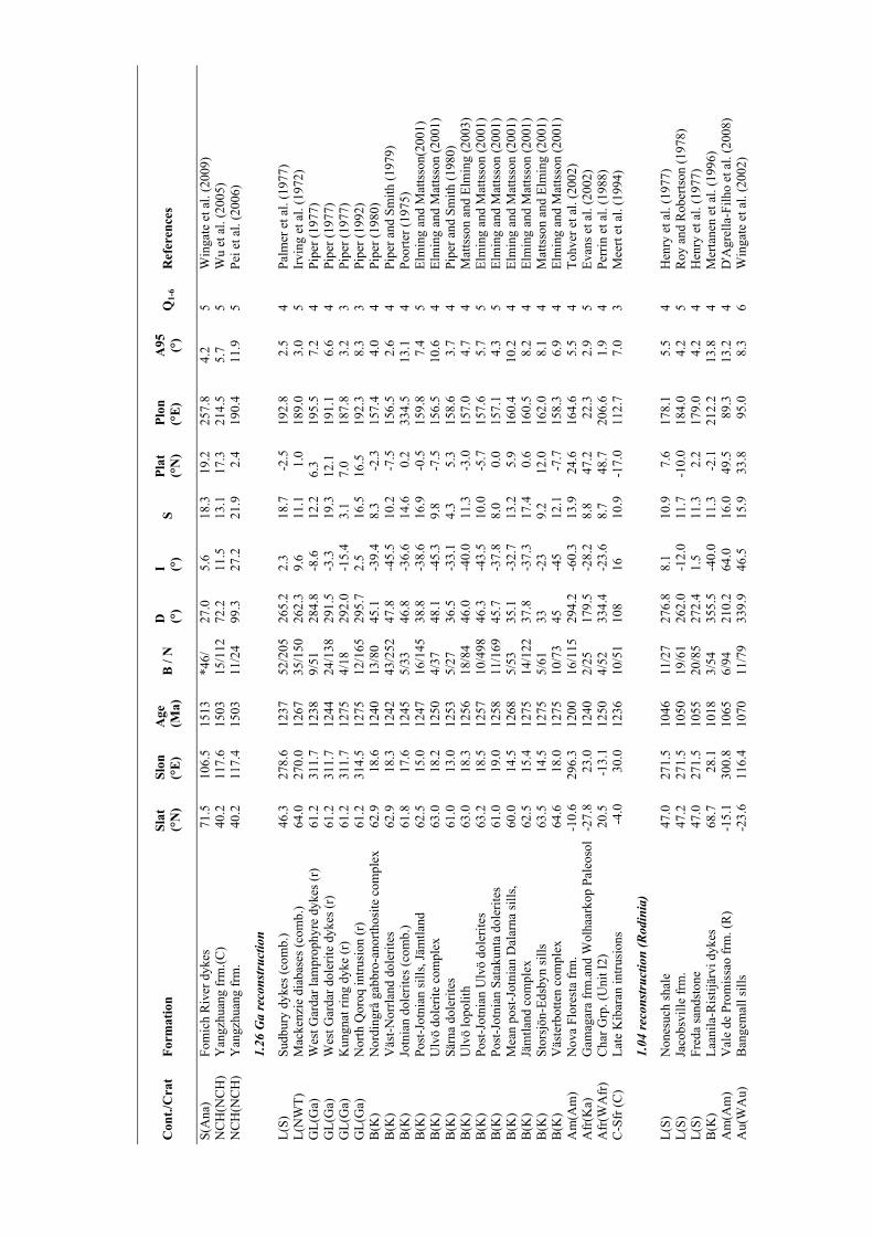
Con

t./C

rat

Form

atio

n Sl

at

(°N

) Sl

on

(°E

) A

ge

(Ma)

B

/ N

D

(°

) I (°

) S

Plat

(°

N)

Plon

(°

E)

A95

(°

) Q

1-6

Ref

eren

ces

S(A

na)

Fom

ich

Riv

er d

ykes

7

1.5

106.

5 15

13

*46/

27

.0

5.6

18.3

1

9.2

257.

8 4.

2 5

Win

gate

et a

l. (2

009)

N

CH

(NC

H)

Yan

gzhu

ang

frm

.(C

) 4

0.2

117.

6 15

03

15/1

12

72.2

11

.5

13.1

1

7.3

214.

5 5.

7 5

Wu

et a

l. (2

005)

N

CH

(NC

H)

Yan

gzhu

ang

frm

. 4

0.2

117.

4 15

03

11/2

4 99

.3

27.2

21

.9

2.

4 19

0.4

11.9

5

Pei

et a

l. (2

006)

1.26

Ga

reco

nstru

ctio

n

L(S

) S

udbu

ry d

ykes

(co

mb.

) 4

6.3

278.

6 12

37

52/2

05

265.

2 2.

3 18

.7

-2.

5

19

2.8

2.5

4

Pal

mer

et a

l. (1

977)

L

(NW

T)

Mac

kenz

ie d

iaba

ses

(com

b.)

64.

0 27

0.0

1267

35

/150

26

2.3

9.6

11.1

1.0

189.

0 3

.0

5 Ir

ving

et a

l. (1

972)

G

L(G

a)

Wes

t Gar

dar

lam

prop

hyre

dyk

es (

r)

61.

2 31

1.7

1238

9/

51

284.

8 -8

.6

12.2

6.

3 19

5.5

7.2

4

Pip

er (

1977

) G

L(G

a)

Wes

t Gar

dar

dole

rite

dyk

es (

r)

61.

2 31

1.7

1244

24

/138

29

1.5

-3.3

19

.3

12.1

19

1.1

6.6

4

Pip

er (

1977

) G

L(G

a)

Kun

gnat

rin

g dy

ke (

r)

61.

2 31

1.7

1275

4/

18

292.

0 -1

5.4

3.1

7.0

187.

8 3

.2

3 P

iper

(19

77)

GL

(Ga)

N

orth

Qor

oq in

trus

ion

(r)

61.

2 31

4.5

1275

12

/165

29

5.7

2.5

16.5

16

.5

192.

3 8

.3

3 P

iper

(19

92)

B(K

) N

ordi

ngrå

gab

bro-

anor

thos

ite

com

plex

6

2.9

18.

6 12

40

13/8

0 45

.1

-39.

4 8.

3 -

2.3

157.

4 4

.0

4 P

iper

(19

80)

B(K

) V

äst-

Nor

rlan

d do

leri

tes

62.

9 1

8.3

1242

43

/252

47

.8

-45.

5 10

.2

-7.

5 15

6.5

2.6

4

Pip

er a

nd S

mit

h (1

979)

B

(K)

Jotn

ian

dole

rite

s (c

omb.

) 6

1.8

17.

6 12

45

5/33

46

.8

-36.

6 14

.6

0.

2 33

4.5

13.1

4

Poo

rter

(19

75)

B(K

) P

ost-

Jotn

ian

sill

s, J

ämtl

and

62.

5 1

5.0

1247

16

/145

38

.8

-38.

6 16

.9

-0.

5 15

9.8

7.4

5

Elm

ing

and

Mat

tsso

n(20

01)

B(K

) U

lvö

dole

rite

com

plex

6

3.0

18.

2 12

50

4/37

48

.1

-45.

3 9.

8 -

7.5

156.

5 10

.6

4 E

lmin

g an

d M

atts

son

(200

1)

B(K

) S

ärna

dol

erit

es

61.

0 1

3.0

1253

5/

27

36.5

-3

3.1

4.3

5.

3 15

8.6

3.7

4

Pip

er a

nd S

mit

h (1

980)

B

(K)

Ulv

ö lo

poli

th

63.

0 1

8.3

1256

18

/84

46.0

-4

0.0

11.3

-

3.0

157.

0 4

.7

4 M

atts

son

and

Elm

ing

(200

3)

B(K

) P

ost-

Jotn

ian

Ulv

ö do

leri

tes

63.

2 1

8.5

1257

10

/498

46

.3

-43.

5 10

.0

-5.

7 15

7.6

5.7

5

Elm

ing

and

Mat

tsso

n (2

001)

B

(K)

Pos

t-Jo

tnia

n S

atak

unta

dol

erit

es

61.

0 1

9.0

1258

11

/169

45

.7

-37.

8 8.

0

0.0

157.

1 4

.3

5 E

lmin

g an

d M

atts

son

(200

1)

B(K

) M

ean

post

-Jot

nian

Dal

arna

sil

ls,

60.

0 1

4.5

1268

5/

53

35.1

-3

2.7

13.2

5.9

160.

4 10

.2

4 E

lmin

g an

d M

atts

son

(200

1)

B(K

) Jä

mtl

and

com

plex

6

2.5

15.

4 12

75

14/1

22

37.8

-3

7.3

17.4

0.6

160.

5 8

.2

4 E

lmin

g an

d M

atts

son

(200

1)

B(K

) S

tors

jön-

Eds

byn

sill

s 6

3.5

14.

5 12

75

5/61

33

-2

3 9.

2 1

2.0

162.

0 8

.1

4 M

atts

son

and

Elm

ing

(200

1)

B(K

) V

äste

rbot

ten

com

plex

6

4.6

18.

0 12

75

10/7

3 45

-4

5 12

.1

-7.

7 15

8.3

6.9

4

Elm

ing

and

Mat

tsso

n (2

001)

A

m(A

m)

Nov

a F

lore

sta

frm

. -1

0.6

296.

3 12

00

16/1

15

294.

2 -6

0.3

13.9

2

4.6

164.

6 5

.5

4 T

ohve

r et

al.

(200

2)

Afr

(Ka)

G

amag

ara

frm

.and

Wol

haar

kop

Pal

eoso

l-2

7.8

23.

0 12

40

2/25

17

9.5

-28.

2 8.

8 4

7.2

22.

3 2

.9

5 E

vans

et a

l. (2

002)

A

fr(W

Afr

) C

har

Grp

. (U

nit I

2)

20.

5 -

13.1

12

50

4/52

33

4.4

-23.

6 8.

7 4

8.7

206.

6 1

.9

4 P

erri

n et

al.

(198

8)

C-S

fr (

C)

Lat

e K

ibar

an in

trus

ions

-

4.0

30.

0 12

36

10/5

1 10

8 16

10

.9

-17.

0 11

2.7

7.0

3

Mee

rt e

t al.

(199

4)

1.04

reco

nstru

ctio

n (R

odin

ia)

L(S

) N

ones

uch

shal

e 4

7.0

271.

5 10

46

11/2

7 27

6.8

8.1

10.9

7.6

178.

1 5

.5

4 H

enry

et a

l. (1

977)

L

(S)

Jaco

bsvi

lle

frm

. 4

7.2

271.

5 10

50

19/6

1 26

2.0

-12.

0 11

.7

-10.

0 18

4.0

4.2

5

Roy

and

Rob

erts

on (

1978

) L

(S)

Fre

da s

ands

tone

4

7.0

271.

5 10

55

20/8

5 27

2.4

1.5

11.3

2.2

179.

0 4

.2

4 H

enry

et a

l. (1

977)

B

(K)

Laa

nila

-Ris

tijä

rvi d

ykes

6

8.7

28.

1 10

18

3/54

35

5.5

-40.

0 11

.3

-2.

1 21

2.2

13.8

4

Mer

tane

n et

al.

(199

6)

Am

(Am

) V

ale

de P

rom

issa

o fr

m. (

R)

-15.

1 30

0.8

1065

6/

94

210.

2 64

.0

16.0

4

9.5

89.

3 13

.2

4 D

'Agr

ella

-Fil

ho e

t al.

(200

8)

Au(

WA

u)

Ban

gem

all s

ills

-2

3.6

116.

4 10

70

11/7

9 33

9.9

46.5

15

.9

33.

8 9

5.0

8.3

6

Win

gate

et a

l. (2

002)

Con

t./C

rat

Form

atio

n Sl

at

(°N

) Sl

on

(°E

) A

ge

(Ma)

B

/ N

D

(°

) I (°

) S

Plat

(°

N)

Plon

(°

E)

A95

(°

) Q

1-6

Ref

eren

ces

Au(

SA

u)

Alc

urra

dyk

es a

nd s

ills

-2

5.9

133.

1 10

73

9/47

29

1.2

50.8

14

.4

2.

8 8

0.4

8.8

4

Sch

mid

t et a

l. (2

006)

S

(Al)

K

umak

ha f

rm.

58.

9 13

5.1

1053

1/

*13

297.

2 3.

9 11

.9

-13.

9 20

1.2

7.0

2

Pav

lov

et a

l. (2

000)

S

(Tu)

L

inok

frm

. 6

6.0

88.

4 10

53

6/*1

39

15.2

-5

7.9

8.6

-15.

2 25

6.2

7.5

6

Gal

let e

t al.

(200

0)

S(A

l)

Mal

gina

frm

. 5

8.3

135.

0 10

53

4/*8

9 99

.7

-42.

0 15

.7

-25.

4 23

0.5

2.8

5

Gal

let e

t al.

(200

0)

S(A

l)

Mil

kon

frm

. 5

8.1

135.

5 10

53

2/*3

3 29

8.7

-18.

5 13

.4

-5.

6 19

5.9

3.9

3

Pav

lov

et a

l. (2

000)

Afr

(Ka)

K

alkp

unt f

rm.

-28.

4 2

1.6

1085

7/

21

170.

0 -7

.0

7.9

57.

0

3.0

5

.3

2 B

ride

n et

al.

(197

9)

I(D

h)

Ana

ntha

pur

alk-

thol

. dyk

es (

E-W

)

14.

1 7

8.3

1026

*8

/>40

65

.2

-57.

0 18

.5

10.

0 21

1.4

12.4

5

Pra

dhan

et a

l. (2

009)

C

-Sfr

(S

fr)

Ilhe

us d

ykes

-1

4.8

321.

0 10

10

17/5

2 60

.0

-66.

8 8.

9 3

0.3

100.

4 4

.0

4 D

'Agr

ella

-Fil

ho e

t al.

(199

0)

C-S

fr (

Sfr

) It

aju

de C

olon

ia d

ykes

-1

5.2

320.

4 10

10

23/6

9 99

.0

-71.

9 25

.8

7.

7 11

1.0

9.8

5

D'A

grel

la-F

ilho

et a

l. (1

990)

C

-Sfr

(S

fr)

Oli

venc

a dy

kes

(N)

-14.

8 32

1.0

1010

31

/93

82.4

-7

1.0

25.6

1

6.1

107.

0 7

.8

4 D

'Agr

ella

-Fil

ho e

t al.

(199

0)

C-S

fr (

Sfr

) O

live

nca

dyke

s (R

) -1

4.8

321.

0 10

10

18/5

4 29

8.8

60.7

19

.9

-9.

5 10

0.2

8.6

4

D'A

grel

la-F

ilho

et a

l. (1

990)

C

-Sfr

(S

fr)

Sal

vado

r dy

kes

(N)

-12.

9 32

1.6

1010

8/

35

110.

8 -7

9.3

22.6

6.4

122.

7 14

.9

5 D

'Agr

ella

-Fil

ho e

t al.

(200

4)

C-S

fr (

Sfr

) S

alva

dor

dyke

s (R

) -1

2.9

321.

6 10

10

7/20

29

0.7

64.7

14

.6

-5.

6 10

2.6

9.2

4

D'A

grel

la-F

ilho

et a

l. (2

004)

C

-Sfr

(S

fr)

Sal

vado

r ba

sic

dyke

s -1

3.0

321.

5 10

20

9/36

99

.0

-79.

1 24

.4

9.

8 12

1.1

16.7

5

D'A

grel

la-F

ilho

(19

92)

NC

H(N

CH

) T

ieli

ng f

rm. (

C)

40.

2 11

7.3

1103

11

/70

296.

3 -4

9.8

42.3

2.2

163.

6 25

.6

4 Z

hang

et a

l. (2

006)

Con

tine

nt (

Cra

ton)

ref

ers

to te

xt a

nd F

ig. 1

. For

mat

ion

give

s th

e ge

olog

ical

roc

k un

it; R

, N, C

in p

aren

thes

is g

ives

the

chos

en p

olar

ity,

whe

re R

(N

) is

rev

erse

d (n

orm

al)

and

C i

s co

mbi

ned

R&

N,

resp

ecti

vely

. ”r

” m

eans

tha

t th

e po

le h

as b

een

rota

ted

due

to P

hane

rozo

ic t

ecto

nic

even

ts:

Gre

enla

nd p

oles

hav

e be

en r

otat

ed r

elat

ive

to L

aure

ntia

usi

ng E

uler

pol

e of

66.

6°N

, 240

.5°E

, rot

atio

n an

gle

-12.

2° (

Roe

st a

nd S

rivi

stav

a, 1

989)

. S

lat,

Slo

n re

fer

to s

ite

Lat

itud

e, s

ite

Lon

gitu

de. B

/N i

s th

e nu

mbe

r of

sit

es/s

ampl

es a

nd *

den

otes

whi

ch l

evel

was

use

d in

Fis

her-

calc

ulat

ions

. D

, I r

efer

to D

ecli

nati

on, I

ncli

nati

on o

f th

e C

hara

cter

isti

c re

man

ent m

agne

tiza

tion

. S is

the

Ang

ular

Sta

ndar

d D

evia

tion

(C

ox, 1

969)

of

the

pole

s as

exp

lain

ed i

n te

xt. P

lat,

Plo

n ar

e la

titu

de, l

ongi

tude

of

the

pale

omag

neti

c po

le. A

95 i

s th

e 95

% c

onfi

denc

e ci

rcle

of

the

pole

. Q1-

6 is

the

tot

al

Q-v

alue

of

six

step

s as

exp

lain

ed in

text

.

Paleo-Mesoproterozoic Supercontinents – A Paleomagnetic Vie · Paleo-Mesoproterozoic...

Documents

Transcript of Paleo-Mesoproterozoic Supercontinents – A Paleomagnetic Vie · Paleo-Mesoproterozoic...