THE INTERNATIONAL RESERVES GLUT: IS IT FOR REAL?

Giulio Cifarelli* Giovanna Paladino**

October 2005

Abstract

Monthly data from January 1985 to December 2004 are used to investigate reserves management in

ten Asiatic and Latin American countries. Idiosyncratic explanatory variables enter cointegration

relationships based on a stochastic buffer stock model, where a reserve variability measure is obtained

via conditional variance approaches. International factors influence the cointegration residuals

(representing the excess demands for reserves), which tend to co-move within and across

geographical areas. Principal components analysis is implemented then to associate their common

drivers with the US fed fund effective interest rate and real effective exchange rate. This two-step

approach sheds light on some controversial aspects of reserves and exchange rate management in

emerging markets such as “fear of floating” and mercantilist behavior. Our results suggest, contrary to

common belief, that the size of recent excess reserves holdings is probably overstated.

Keywords: emerging markets’ international reserves, cointegration analysis, principal components analysis. * University of Florence, Economics Department, via delle Pandette 9, 50127 Florence, Italy. giulio.cifarelli@unifi.it ** LUISS University and Sanpaolo IMI Economic Research Dept., viale dell’Arte 25, 00144 Rome, Italy. giovanna.paladino@sanpaoloimi.com

The average reserve holdings of several emerging markets have risen in recent years,

irrespectively of their official exchange rate regime, both in absolute terms and as percentages

of GDP or of standard international trade and finance adequacy indicators, such as the level of

imports or the short term external debt. They have reached $1.8 trillion at the end of 2004, up

roughly $800 billion from 2002 and more than four times their level in 1994, exceeding the

potential requirements of any foreseeable shock. So what is the purpose of possessing

international reserves in excess of common measures of adequacy? This puzzle has attracted

considerable attention from both practitioners and academics. Precautionary behavior of

central banks, fear of the disruptive effects of an exchange rate depreciation (motivated by the

experience of the financial crises and sudden capital reversals of the 1990s), difficult access to

international capital markets and mercantilist export support are possible explanations set out

in a burgeoning literature.

In this paper monthly data from January 1985 to December 2004 are used to investigate the

national idiosyncratic and international determinants of reserve changes in five Asiatic and

five Latin American countries. Idiosyncratic explanatory variables are mostly associated with

the tenets of the benchmark buffer stock model of Frenkel and Jovanovic (1981) while

international explanatory factors reflect the pivotal role played by the U.S. monetary

authorities in emerging markets finance.

The use of a monthly frequency has a number of drawbacks due to the non stationary nature

of the time series and to the difficulty of estimating consistent cointegration relationships and

error correction structures. The twenty year data span, however, provides a large number of

observations and allows to estimate the relevant relationships for each country in isolation.

Most previous empirical studies (Flood and Marion, 2002, Aizenman and Marion, 2004,

among others) are performed with yearly data and rely on the panel data approach. The latter

posits that the specification of the relationship is the same over the cross section and that any

idiosyncratic effect is adequately captured by differences in the constant term. In the present

investigation, however, the specification of the demand for reserves, the sign and the

significance of the coefficients and the speed of convergence to equilibrium differ too much

across the countries of the sample to be properly assessed using a pooled data procedure. A

different estimation methodology is called for.

1

The rapid growth of short term capital flows provides a sensible explanation for the relevance

of the precautionary demand for reserves of the buffer stock model. Capital flows to and from

emerging markets, however, have specific characteristics that go beyond the standard

approach. According to the buffer stock model international reserves are explained by

domestic factors only, reserve volatility and a national bond yield which reflects the

opportunity cost of holding them. This parameterization misses some relevant determinants of

reserve behavior. International financial flows involving emerging markets are highly volatile

and are affected by US monetary policy. Over the last two decades convincing evidence

shows that financial turbulence (and the ensuing impact on reserve holdings) is not restricted

to the epicentre of a crisis but tends, usually, to spread from country to country within and

even across geographical areas. The two-step estimation procedure implemented in this paper

is meant to capture these aspects of emerging markets finance.

Cointegration reserve relationships are independently estimated, at first, for each country. The

corresponding residual time series are assumed to quantify the fraction of the long run reserve

holdings which cannot be explained by the buffer stock model explanatory variables.1 Their

correlation is carefully analyzed in a second step and the relevance of common drivers is

assessed using principal components analysis. Geographical area co-movements are

identified; the behavior of the first principal component - which explains almost 40 percent of

the variability of the residuals of the Asiatic reserve cointegration relationships - turns out to

be affected by the U.S. federal funds and real effective exchange rate.

The signs of the estimated coefficients suggest that reserve residual co-movements reflect

both the generalized impact of U.S. monetary policy due to a “fear of floating” reaction

(Calvo and Reinhart, 2002) and a common desire to prevent real exchange rate appreciation.

The latter may be related to an export support mercantilist exchange rate policy (Aizenman

and Lee, 2005 ).

The paper improves upon previous research in the following aspects:

1 The two-step approach fits well with the model of Frenkel and Jovanovic which posits that observed reserves are proportional to optimal reserves – determined according to the buffer stock paradigm – up to an error term that is uncorrelated with the determinants of the latter. Optimal reserve holdings are the fitted values of the cointegration relationships.

2

- the empirical section includes an accurate analysis of the time series; additive outliers that

may affect both the unit root tests and the cointegration results are disposed of using

approaches set forth by Perron and Rodríguez (2003) and Nielsen (2004).

- Reserves volatility clustering is modelled using conditional volatility techniques; the

IGARCH parameterizations produced by the data suggest that the volatility estimates in

previous research, that relied on unconditional variance estimation, may well be biased.

- The two-step estimation approach sheds light on some controversial aspects of exchange

rate management, such as “fear of floating” and mercantilist behavior. A distinction is

drawn between the national (idiosyncratic) and the international factors that affect reserve

holdings. The former enter the long run cointegration relationships while the latter

influence the disequilibrium residuals, which tend to co-move across countries. Principal

components analysis is then used to associate their common drivers to US monetary and

exchange rate policy.

- Contrary to common belief and, indeed, to the implications of standard adequacy

measures, our analysis suggests that current excess reserve holdings are not consistently

larger than their 1995-2004 averages.

The paper is structured as follows. Section 1 summarizes the theoretical and empirical

discussion on reserve adequacy rules and on optimal reserve holdings; section 2 measures

reserve excess demand, using rules of thumb and cointegration analysis; section 3 investigates

excess reserve co-movements and assesses the relevance of “fear of floating” and of

mercantilist export support policies. Section 4 concludes the paper.

1 The demand for international reserves

In this section the literature on the demand for international reserves is briefly summarized.

The structure of the dynamic stochastic model set forth by Frenkel and Jovanovic (1981) is

then examined in more detail as it constitutes the theoretical framework of the applied

analysis of the subsequent sections.

3

1.1 From rules of thumb to optimal reserve management

An adequate stock of reserves is assumed to finance potential gaps between outlays and

receipts of foreign currency, smoothing out external payment imbalances and preventing in

that way an exchange rate crisis. It is typically determined by a ratio between the minimum

amount of reserves the authorities have to hold on average and a component of the balance of

payments. In the 1950s and 1960s the trade balance was the largest aggregate of the latter and,

according to standard Keynesian macroeconomics, reserves were geared to imports. Studies

by the IMF Staff (1958) and Triffin (1960) suggested that reserve adequacy required a

minimum average yearly reserve to import ratio of 30-35 percent.

The relative marginalization of trade aggregates in the overall balance of payments accounts

brought about by the liberalization of capital flows in the 1980s and 1990s called for the

introduction of a more effective rule of thumb. It was suggested that since recent currency

crises tended to be associated with capital outflows rather than with trade financing, the size

of the reserves of emerging market economies be somehow related to their short run external

debt outstanding. The Asian crisis had shown that the countries that held large reserves had

been able to weather the turbulence better than the others.2

Two proposals for a new minimum reserve stock benchmark were set out in 1999,

respectively, by Pablo Guidotti, Argentina’s former Deputy Minister of Finance, and Alan

Greenspan, Chairman of the US Federal Reserve Board, both involving short term emerging

market debt.

Guidotti proposed, as an empirical rule of thumb for reserve stock adequacy, that a country be

able to satisfy its net external payments liabilities without additional foreign borrowing for up

to one year. The current account deficit is thus included in this reserve adequacy criterion

along with short term debt. In a similar way Greenspan suggested to calibrate reserve

adequacy on short term debt outstanding with maturity of less than one year. He introduced,

however, two additional conditions: (i) that the average maturity of a country’s external

2 A link has been identified in a recent IMF study (IMF, 2000) between short term debt over reserves and the likelihood of a crisis in a sample of emerging market economies. In the same way Early Warning System studies by Bussière and Mulder (1999), among others, have found that low reserve to short term external debt ratios increased the probability of a crisis.

4

liabilities exceed a three year threshold and (ii) that the reserve authorities operate following a

“liquidity at risk” procedure.

A third reserve adequacy criterion is the reserve to broad money (M2) ratio. Kaminsky et al.

(1997), among others consider it an accurate predictor of crises. De Beaufort Wijnholds and

Kapteyn (2001) point to the usefulness of this ratio for assessing the relevance of internal

demand for foreign reserves due to possible capital exports by domestic residents.

In an authoritative study Heller (1966) went beyond reserve adequacy and analyzed

precautionary optimal reserve management by monetary authorities. International liquid

reserves allow to finance external imbalances and to avoid deflationary measures with a

relevant macroeconomic cost. Reserve holdings, however, have an opportunity cost given by

the difference between the social yield on capital invested and the (lower) yield of

international reserves. The optimal stock of reserves corresponds to the amount which

minimizes the sum of the cost of adjusting for and of financing the balance of payments

disequilibrium in such a way that the marginal cost of the former equals that of the latter. The

analysis of Heller is relevant also from a formal point of view.3 In spite of the shortcomings

pointed out by Hamada and Ueda (1977), it provides the basic original framework for most

subsequent theoretical and empirical research on optimal foreign reserve management.

1.2 The stochastic buffer stock model of the demand for reserves

Extending a previous model on transactions and precautionary demand for money, Frenkel

and Jovanovic (1981) set forth a stochastic reformulation of optimal reserve demand based on

the tenets of inventory management. Their model posits that changes in reserve holdings,

between restockings, be modelled by the following stochastic equation

dR dt dWt = − + tµ σ (1)

3 He assumes that the process of change in the stock of international reserves is a random walk and provides an algebraic formulation which links the optimal amount of reserves a country should hold to the propensity to import, the opportunity cost of holding reserves and to a proxy for the stability of its international accounts, as reflected by the average yearly past imbalances.

5

where is a Wiener process with mean zero and variance t. At any point in time the

distribution of the reserve holdings reads as

Wt

R R Wt = − +0 tµ σ (2)

where is the optimal initial stock of reserves, R0 µ is a drift parameter and σ is the standard

deviation of the Wiener reserve increment. Optimal reserve management involves the

selection of the cost minimizing stock of reserves once reserves have reached a lower bound,

set here to zero. Since reserve holdings follow a stochastic process, the authorities are

assumed to select the initial level of reserves that minimizes total expected costs. Costs

here have two interrelated components : (i) the opportunity cost of reserve holdings and (ii)

the adjustment cost of reserve restocking whenever the latter have reached their lower bound.

The latter stems from the output (welfare) reduction brought about by the need to generate the

balance of payments surplus, which will generate the reserve build up.

R0

Frenkel and Jovanovic assume that balances of payments tend on average to be in equilibrium

and that the reserve drift between restockings µ is zero. They obtain, after some algebraic

manipulation, the following second order Taylor series approximation of optimal initial

reserve holdings in logarithmic terms

log . log . logR c0 05 0 25= + − rσ (3)

The crucial additional assumption is then made that observable reserves are proportional

to optimal (initial) reserves up to an error term that is uncorrelated with

Rt

σ and r. The

following testable relationship is then derived

log log logR b b b r ut t= + t t+ +0 1 2σ (4)

where it is assumed a priori that b and b1 0> 2 0< .4

4 Flood and Marion (2002) argue that optimal and observed reserves are linked by the relationship , where B is a country specific proportionality factor.

R BR etut= −

0

6

Reserve holdings at time t are reduced if the opportunity cost r rises and increased whenever

their volatility

t

σ t rises. A higher volatility implies that holdings are likely to hit their lower

bound more frequently and require costly restockings that the authorities want to avoid.

The resurgence of interest for reserve hoarding management in the aftermath of the financial

crises of the 1990s has prompted various attempts to adapt precautionary demand modelling

to the financial characteristics of emerging market countries. The latter have to face a limited

access to international borrowing in periods of stress, an inefficient tax collection system and

- at times – a severe default risk. Reserves are assumed to have an insurance value. Aizenman

and Marion (2004), using a two period intertemporal consumer utility maximization model,

suggest that reserves reduce the cost of consumption smoothing between prosperous and bad

states of nature. In the latter the marginal cost of public funds would be much higher.

Subsequent studies focus on an output stabilization role of international reserves. Aizenman et

al. (2004) show that reserve holdings mitigate the probability of a banking crisis and thus

reduce the expected output costs of a sudden freeze of international capital inflows. Their

demand for reserves increases both with the expected output cost of a credit crisis and with

the effectiveness of reserves in reducing the probability of the crisis. As shown in Aizenman

and Lee (2005) a macro liquidity shock to an emerging market cannot be diversified away and

may force the liquidation of a first period investment if it exceeds the stock of reserves

outstanding, reducing second period output. Optimal reserve management diminishes

potential liquidation costs.

1.3 Empirical investigation on precautionary reserves management

A large body of empirical research relies on the buffer stock model paradigm, spanning more

than twenty years – see Bahmani-Oskooee and Brown (2002) for a comprehensive survey.

Reserves are typically linked to four regressors in a panel data study: a variability measure,

the marginal (or average) propensity to import, the level of imports and an opportunity cost

proxy.

It is generally found that net external payments variability exerts a positive and significant

impact on reserve holdings; the demand for the latter increases with the fluctuations in the

balance of payments, quantified in various ways by a variability index.

7

The sign of the coefficient of the second regressor, the propensity to import, is more

controversial. On Keynesian grounds it should be negative; the larger the propensity to

import, the smaller the adjustment cost when expenditure reduction policies are called for and

the smaller the demand for reserves (Heller, 1966). If, however, the propensity to import is

assumed to quantify a country’s openness and vulnerability to external shocks, the sign of the

coefficient should be positive as more reserves are required whenever the propensity rises

(Aizenman and Lee, 2005).

The third regressor, the value of imports, is positively related to the demand for reserves. It is

believed to measure the effects of trade and is used as a scale variable.5 Indeed Heller (1968),

assumed that banks’ transactions demand for foreign exchange increased with the square root

of the level of transactions. De Beaufort Wijnholds and Kapteyn (2001) point out that the

presence of economies of scale (which justify the use of imports as scale variable) hinges on

the hypothesis that balance of payments disequilibria grow in proportion to international

transactions.

The opportunity cost of holding reserves has been measured in various ways. Frenkel and

Jovanovic (1981) used government bond yields and Edwards (1985), among many others,

spreads between domestic and corresponding US interest rates. The negative coefficient of the

opportunity cost regressor is seldom significantly different from zero, a finding that can be

attributed to the risk averse nature of central banks.

The choice of the variables entering the cointegration analysis performed in the paper - as the

first step of the estimation procedure - is broadly in line with the above mentioned research.

Long run reserve demand is assumed to be related to a variability index, the level of imports

and to a long term bond yield. The average propensity to import is dropped from the analysis.

The problems associated with openness and external vulnerability are dealt with in the second

step.

2 Assessment of the excess demand

One of the main lessons to be drawn from the Asian and Latin American crises is that fear of

insolvency may trigger sudden and dangerous capital reversals even in countries that do not

8

seem to have - prima facie – serious debt sustainability problems. Reserve and debt

management are thus key factors in crisis prevention.6 Holding foreign assets is costly and

while the case for Central Bank reserve accumulation is evident, it is still not clear what is

their optimal level. Indeed, some countries seem to have an insatiable appetite for reserves as

if “Mrs Machlup’s wardrobe theory” were to hold.7

In this section measurements of excess reserve demand are set forth for ten countries located

in Asia and in Latin America using two alternative approaches.

2.1 Stylized evidence from the rules of thumb

In the absence of a widely accepted theoretical approach to optimal reserve size, popular rules

of thumb, summarized in section 1.1 above, have supplied guidance to central bankers.

[Insert Table I]

The computation of five different reserve adequacy benchmarks for Argentina, Brazil, Chile,

Mexico, Venezuela, Indonesia, Korea, Malaysia, the Philippines and Singapore is set forth in

table I. The description and the sources of the time series used in the empirical analysis can be

found in Appendix I.

The first benchmark is measured in terms of month worth of imports. It can be seen –

according to a balance of trade and/or a consumption smoothing criterion – as a way to ensure

a certain degree of autonomy from scarce international borrowing. International reserves are

thus required to cover 4 to 6 months of imports. This index has lost most of its relevance over

time as emerging economies increasingly rely on private capital flows to balance their

external accounts. The Guidotti rule discussed above is motivated by this development and by

evidence that vulnerability, during the Asian crisis, was mainly related to a country’s asset

and liquidity management. It provides a benchmark based on a ratio of reserves to short term

debt and is meant to gauge the capability of a country to live without foreign borrowing for up

to a year (in that case the reserve adequacy ratio would be 100 per cent). The third column 5 A positive coefficient, smaller than one in absolute value, would signal the presence of economies of scale. Real GDP, real GDP per capita or population size are also used as scaling variables. 6“…..We have also seen in the recent crises that countries that had big reserves by and large did better in withstanding contagion than those with smaller reserves..” , (p.1-3). Fischer, S. (2001). ‘Opening Remarks’, IMF/World Bank International Reserves: Policy Issues Forum (Washington, DC, April 28).

9

expands the Guidotti rule and incorporates an additional cushion of 3 percent over and above

short term external debt in order to buy time for the required policy change before the

reserves to short term debt threshold is reached (Bird and Rajan, 2002).

De Beaufort Wijnholds and Kapteyn (2001) argue that a reserve to short term debt ratio may

fail to capture the threat of an “internal drain” due to capital exports by residents. Capital

flights are accounted for with greater accuracy by the measure based on broad money supply

(M2) of column four. The ratio of reserves to M2 should be close to 30 percent as only a

fraction of M2 may realistically be expected to be mobilized on short notice.

The last index too takes into account both internal and external capital drains. It is based on

the Greenspan “liquidity at risk” refinement of the Guidotti rule.8 We implement here the

version set out by De Beaufort Wijnholds and Kapteyn (2001). The denominator of the

Guidotti rule is modified introducing a “probability factor” which depends on a country risk

index weighted according to the exchange rate regime. The ratio is fully explained in the

notes to table I.

This table sets forth adequacy measures computed for the years 1985, 1995 and 2004. They

are underlined if the estimates exceed the corresponding adequacy benchmarks. The reserve

to import ratios record a net improvement over time, with the exception of Mexico and the

Philippines, where the increase is less relevant. As for the remaining indexes, they suggest

that all the countries in the sample currently hold reserves that are significantly above the

adequacy thresholds set at 100 percent and 30 percent for, respectively, the Guidotti and

Guidotti-Greenspan rules and for the reserve to M2 ratio. Our findings so far, in line with the

common wisdom, support the hypothesis of a generalized increase in reserve holdings from

1985 to 2004.

2.2 Long-run demand and reserves misalignment

Conventional adequacy rules are simplistic by construction and may underestimate emerging

markets reserve requirements. This section describes the econometric strategy used to

7 Professor Machlup suggested that monetary authorities tended to maximize the stock of reserves as his wife was maximizing the amount of clothes in the wardrobe. 8 A. Greenspan (1999). ‘Currency Reserves and Debt’, remarks at the World Bank Conference on Trends in Reserve Management (Washington, DC, April 29).

10

determine the optimal long run demand for reserves. This measure of reserve adequacy

evolves over time and provides a dynamic benchmark that can be used to assess the relevance

of overstocking. The optimal buffer stock model demand for reserves, discussed in section

1.2, is estimated using Johansen’s (1988, 1991) cointegrating approach. The data set spans the

January 1985 - December 2004 time period and encompasses some important episodes of

distress both in Asia and Latin America.

2.2.1 Stationarity and volatility analysis

Recent econometric findings summarized in Vogelsang (1999) have shown that additive

outliers introduce in the residuals of standard unit root test estimates a moving average

component with a negative coefficient which, in turn, inflates the size of the test and causes

over-rejection of the null hypothesis. The Latin American and Asiatic crises have brought

about long lasting changes in Central Bank behavior and the corresponding outliers in the

time series may well be considered additive in the sense of Hendry and Doornik (1994). We

have implemented the test procedure of Perron and Rodríguez (2003) and have identified

several additive outliers. The value of the test statistics that are significant at the 5 percent

level and the corresponding dates are set out in Appendix II. The unit root tests of table II are

thus performed using the statistic by Ng and Perron (2001), which is robust to size distortions

due to negative serial correlation of the residuals. With one single exception, they fail

systematically to reject the null of non stationarity.

[Insert table II]

Additive outliers may also distort inference on cointegration rank in finite samples (Franses

and Haldrup, 1994). Following the interpolation strategy suggested by Nielsen (2004), the

outlying observations are eliminated and replaced by an average of the respective adjoining

data. The smoothed time series will then be used in the cointegration analysis below.

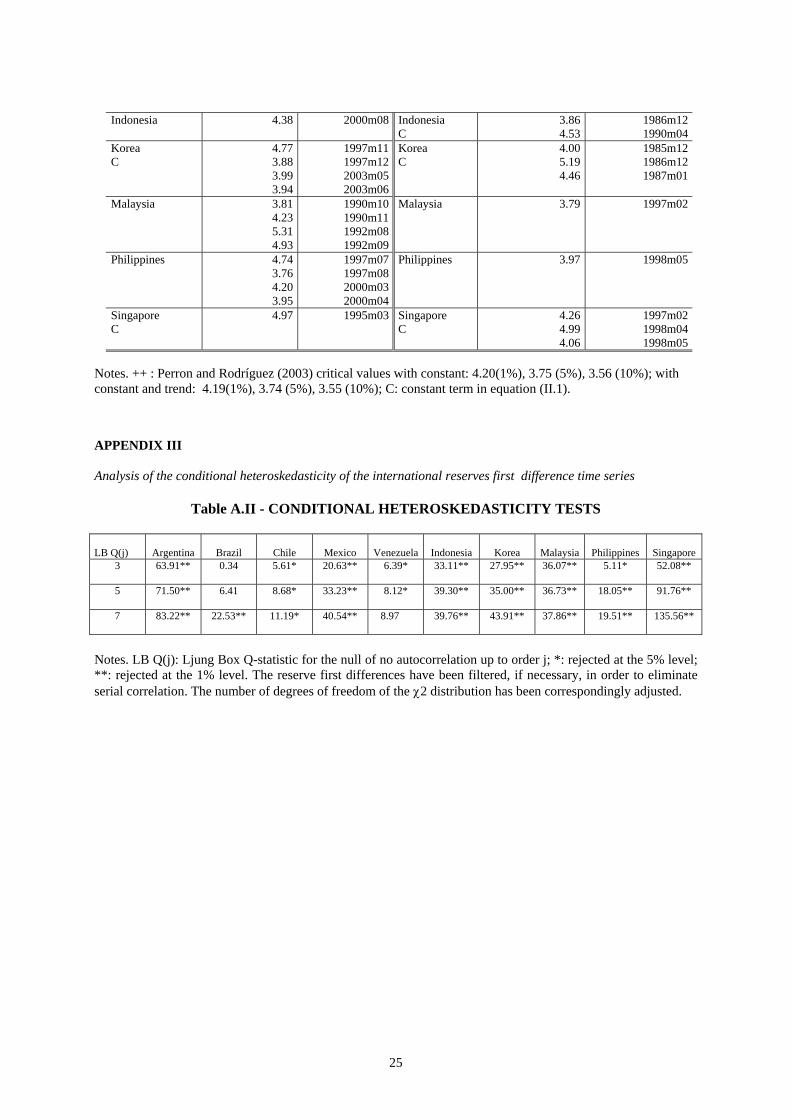
Reserve volatility plays a relevant role in models of optimal demand for foreign reserves and

has to be carefully estimated. Most previous empirical studies borrow a method originally

developed by Frenkel (1974) and estimate reserve volatility as a multiperiod rolling standard

11

deviation of (detrended) reserve changes.9 Our sample period includes periods of turbulence

and reserve changes display volatility clustering i.e. autoregressive conditional

heteroskedasticity. The presence of ARCH effects is corroborated by the serial correlation of

the squared reserve increments. Indeed, almost all Ljung Box Q-statistics in table A.II reject

the null of no ARCH at the standard levels of significance. Unbiased volatility estimates are

thus obtained using conditional measures, computed as the square root of the GARCH(1,1)

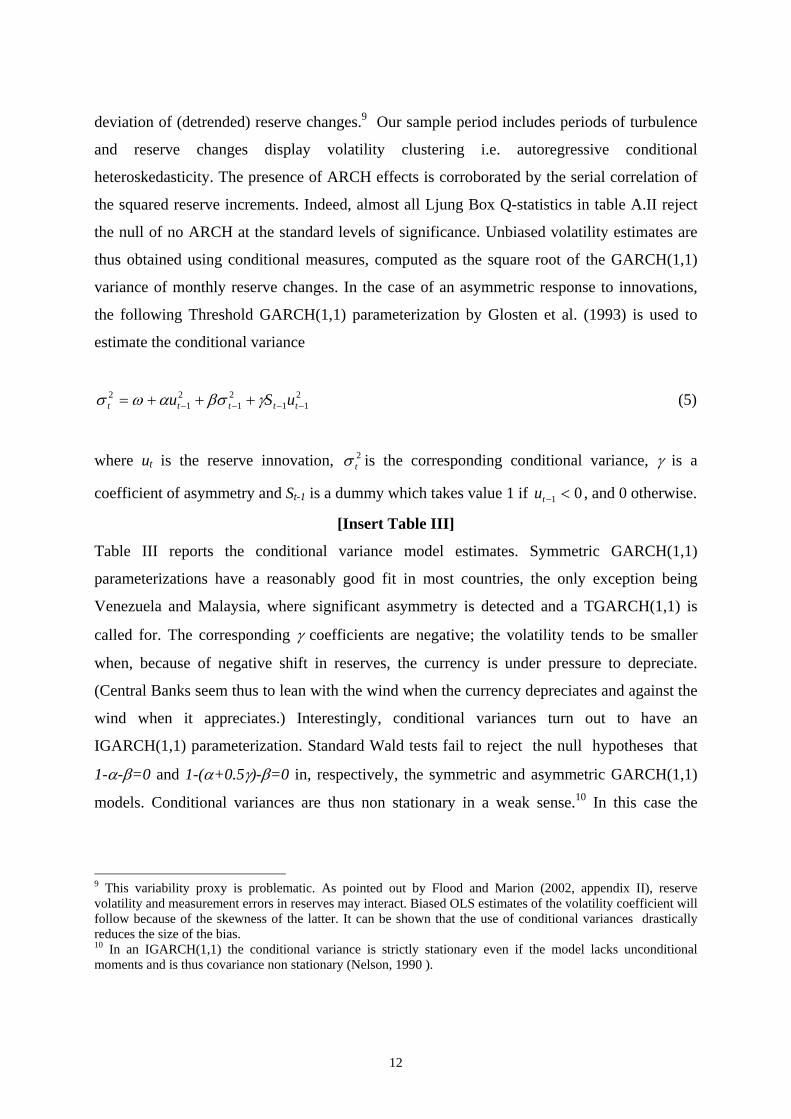
variance of monthly reserve changes. In the case of an asymmetric response to innovations,

the following Threshold GARCH(1,1) parameterization by Glosten et al. (1993) is used to

estimate the conditional variance

σ ω α βσ γt t t tu S21

21

21 1

2= + + +− − − tu −

(5)

where ut is the reserve innovation, is the corresponding conditional variance, γ is a

coefficient of asymmetry and S

2tσ

t-1 is a dummy which takes value 1 if u , and 0 otherwise. t− <1 0

[Insert Table III]

Table III reports the conditional variance model estimates. Symmetric GARCH(1,1)

parameterizations have a reasonably good fit in most countries, the only exception being

Venezuela and Malaysia, where significant asymmetry is detected and a TGARCH(1,1) is

called for. The corresponding γ coefficients are negative; the volatility tends to be smaller

when, because of negative shift in reserves, the currency is under pressure to depreciate.

(Central Banks seem thus to lean with the wind when the currency depreciates and against the

wind when it appreciates.) Interestingly, conditional variances turn out to have an

IGARCH(1,1) parameterization. Standard Wald tests fail to reject the null hypotheses that

1-α-β=0 and 1-(α+0.5γ)-β=0 in, respectively, the symmetric and asymmetric GARCH(1,1)

models. Conditional variances are thus non stationary in a weak sense.10 In this case the

9 This variability proxy is problematic. As pointed out by Flood and Marion (2002, appendix II), reserve volatility and measurement errors in reserves may interact. Biased OLS estimates of the volatility coefficient will follow because of the skewness of the latter. It can be shown that the use of conditional variances drastically reduces the size of the bias. 10 In an IGARCH(1,1) the conditional variance is strictly stationary even if the model lacks unconditional moments and is thus covariance non stationary (Nelson, 1990 ).

12

unconditional variance of reserve innovations is not defined and the conditional GARCH

approach provides the only meaningful measure of reserve volatility.

2.2.2 Cointegration estimates of long run reserves demand

The empirical investigation is performed using the multivariate cointegration analysis of

Johansen (1988, 1991). The selection of this approach is not arbitrary. It is motivated by its

resilience in terms of power and of size to the conditional heteroskedasticity of the VECM

residuals detected by Boswijk et al. (2000).11

[Insert table IV]

The trace test statistics set forth in table IV identify a single cointegration relationship in each

of the ten countries. The treatment of the deterministic component is not homogeneous and

reflects the differing properties of the time series.

Table V presents the cointegration equation estimates and the corresponding error correction

coefficients obtained with the FIML procedure of Johansen and Juselius (1990). The short

term components of the VECM are not set forth here for lack of space. The long run reserve

demand relationship is formulated as

log log $ log logR t M rt t t− − − − t t− =ρ ρ β σ β β ε0 1 1 2 3 (6)

where $σ t is the fitted value of a preliminary IGARCH conditional volatility estimate of the

reserve change, is the volume of imports, r is the domestic (US dollar denominated)

government bond yield and t is a time trend.

Mt t

[Insert table V]

11 They perform a Monte-Carlo comparison of the Johansen LR cointegration test and of alternative LM approaches that try to exploit the non-normality of the residuals in the case of Gaussian and non-Gaussian distributions of the VECM innovations. The Gaussian QLR test of Johansen loses power in the presence of skewness and of flat tailedness. It turns out, however, to outperform the alternative cointegration tests when the innovations exhibit, a major problem in our empirical analysis, GARCH(1,1) volatility clustering (see table 1, pages 15-16). The sizes of the cointegration tests are not seriously affected by non-Gaussianity but for the rather unrealistic case of an ARCH(1) parameterization of persistent conditional volatility.

13

The estimates are far from homogeneous across countries.12 The computed values of the

coefficients of reserve volatility and of the opportunity cost proxy corroborate the

specification of the buffer stock model only in the case of the Asiatic countries. A rise in

interest rates is associated with an increase in reserve holdings in three of the five Latin

American countries, possibly reflecting - as suggested by Aportela et al. (2005) - the effect of

foreign capital inflows sterilization policies by local monetary authorities. Reserve volatility

too does not fit well with the model in Latin America: with the exception of Venezuela it is

either irrelevant or has a negative impact on the demand for reserves. Only the coefficient of

the volume of imports is significant and has the appropriate sign in most countries of the

sample. With few exceptions, its size fails to support the hypothesis of economies of scale in

the use of reserves, a finding that may be due to the impact of the introduction of reserve

adequacy rules geared on imports.

The error correction terms, finally, are – with two exceptions, Malaysia and the Philippines –

significant and of the correct sign. Rather small in absolute value, they suggest that it might

take long time for the reserve equations to return to equilibrium after a shock.

3 Excess reserve co-movements and international capital markets integration

Standardized cointegration residuals in figures 1 and 2 show that the amount of recent excess

reserve holdings may well be overstated. Contrary to common belief - and, indeed, to the

implications of the adequacy thresholds of table I - emerging market countries’ Central Banks

do not seem to have modified their behavior in recent years since excess reserve holdings are

not consistently larger than their 1995-2004 averages.

[Insert Figure I]

[Insert Figure II]

Having singled out the idiosyncratic factors that determine, in each country, the precautionary

demand for reserves, we investigate the co-movements among the cointegration residuals in

order to assess the relevance of common international drivers on reserve overstocking.

Factors that influence international capital and trade flows are likely to affect 12 The differences involve the sign, absolute value and significance of the coefficients of most regressors and are not restricted to the constant term. These findings suggest that a panel data procedure would be misleading if applied to our data set.

14

contemporaneously the entire set of countries of the sample. The size of the cross country

correlation coefficients reported in table VI is indicative of a common element among the

estimates of excess reserve holdings.

[Insert Table VI]

3.1 Principal components analysis

Principal components analysis (PCA) allows to investigate the pattern of the co-movements in

reserve misalignments. Exploiting the potential information redundancy in multivariate data

sets, PCA reduces the dimensionality of the data with minimal loss of information. It

transforms a set of N correlated variables (the Johansen cointegration residuals) into a smaller

subset of M ≤ N uncorrelated variables (principal components) that are orthogonal linear

combinations of the original ones. The first component will have the maximum possible

variance, the second the maximum possible variance among the linear combinations

uncorrelated with the first principal component and so on.

Let be a Tx1 vector of cointegration residuals and N,...,i,yi 1= iiii )yy(x σ−= be the

corresponding standardized residual vector where iy and iσ are the unconditional sample

mean and standard deviation. is a column of the TxN matrix, X, of standardized excess

reserve time series. Principal components analysis is based on the eigenvalue eigenvector

decomposition of the (correlation) matrix

ix

T/X'X=Σ .

The principal components transformation of X reads as

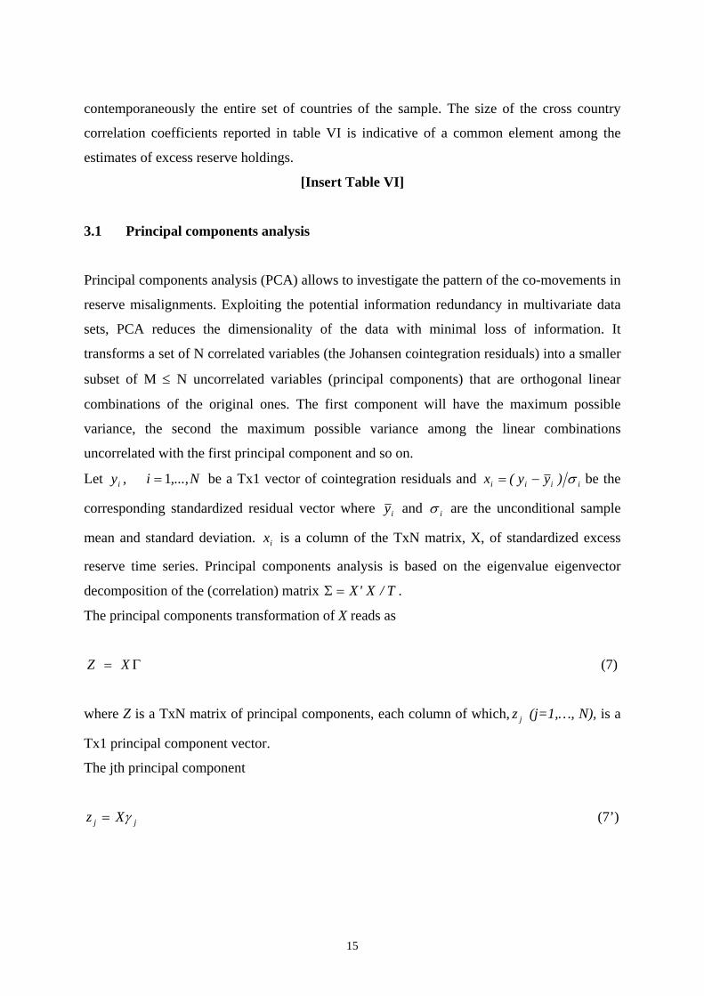
Γ= XZ (7)

where Z is a TxN matrix of principal components, each column of which, (j=1,…, N), is a

Tx1 principal component vector.

z j

The jth principal component

z Xj = jγ (7’)

15

has zero mean and variance λ j . With the latter appropriately normalized it is possible to

measure the fraction of the variance of the original data explained by the corresponding

principal component. Similarly, the sum of the first M normalized eigenvalues indicates how

much variation is explained by the first M principal components.

Consistent estimation of the correlation matrix and of the corresponding principal components

requires that the time series be stationary. This is the case here since cointegration residuals

are stationary by construction.

PCA, implemented on excess reserve holdings, shows that the first principal component may

explain up to 38 percent of the variability of the residuals of the reserve cointegration

relationships in the case of Asia. The first three principal components explain 60 to 85 percent

of the excess reserve variability in the single area and cross area estimates.

[Insert Table VII]

3.2 Fear of floating and mercantilist factors affecting reserve holdings

The remaining issue is whether there are international drivers able to explain the behavior of

the identified common patterns (principal components) among excess reserve holdings. This

section presents the economic rationale and the empirical evidence supporting the hypothesis

that the US policy rate and the US dollar real effective exchange rate are key international

factors driving Central Banks’ decisions to accumulate reserves beyond their optimal level.

Recent global economic integration has offered interesting financing opportunities but has

also increased the exposure of emerging countries to contagion and to inflation pass through.

Several studies suggest that capital flows are driven by common international factors. As

shown by Calvo et al. (1996) and Mody et al. (2001), among others, shifts in US monetary

policy influence emerging markets financial liquidity. A tight US monetary policy makes

investment in these countries less attractive, raising debt price. The corresponding increase in

the rate of interest differential results in cross border financial flows.13

The extent to which the local monetary authorities react to changes in the US interest rate

depends, in principle, on the nature of the exchange rate arrangements. Under a pegged

16

exchange rate regime the reaction would be strong, in order to avoid the insurgence of a risk

premium. Under floating regimes, changes in international interest rates could be

accommodated through exchange rate movements. Frankel (1999), however, found that also

in free floating countries (such as Brazil and Mexico) an increase in the fed fund rate brings

about a more than proportional increase in the domestic interest rate. The latter is due to the

large effect of interest rate differentials on capital outflows and to the required large premium

for devaluation and default risk.

This picture is not exhaustive since the monetary policy framework matters as well. Under an

inflation targeting regime, even in the case of free floating exchange rates, an increase in the

US interest rate may cause a depreciation of the national currency (because of lower capital

inflows or capital reversals towards higher US risk adjusted returns) and the authorities will

be willing to reduce liquidity, trading off economic growth with inflation. This fear of floating

can be faced, alternatively, increasing the foreign reserve holdings above precautionary levels.

In general, a large buffer for future exchange market intervention reduces the degree of

external vulnerability to contagion. International linkages among monetary policies may thus

influence the strategies of Central Banks directly through the interest rate and indirectly via

reserve holding decisions. If, according to the empirical evidence mentioned above, a US

monetary policy tightening has an adverse effect on emerging market financial stability, we

expect a positive relation between the US fed fund effective rate and reserve overstocking.

Purchases of foreign currency during a period of upward pressure on the domestic exchange

rate and rather limited intervention on the downside are consistent with an attempt to avoid a

deterioration of national competitiveness i.e. with a deep-rooted mercantilist desire to

maintain an undervalued exchange rate. This explanation agrees with the suggestion of

Dooley at al. (2003) that emerging countries build up reserves in order to support their

exports. A sensible development strategy might then require a distortion in the real exchange

rate in order to channel domestic investment towards export industries and a process of

reserve accumulation, which would appear sub-optimal, is in reality an element of an optimal

investment strategy.

13 See Arora and Cerisola (2001) and Uribe and Yue (2003). It is also believed that US monetary policy plays a relevant role in triggering financial and banking crises since a rise in industrial country interest rates worsens the conditions for the access of emerging markets to offshore funds.

17

The depreciation of the US real effective exchange rate is used here as a synthetic (global)

measure of domestic foreign exchange pressure due to trade. Thus a depreciation, i.e. a

negative shift, in the US real effective exchange rate has to be associated with an increase in

excess reserve holdings. Emerging market Central Banks buy foreign assets and sell domestic

ones in order to avoid a reduction of domestic competitiveness through an undesired

exchange rate appreciation.14

In this section empirical evidence on the impact of the selected international factors is

provided by regressing the first principal component of the interregional and of the two

regional sets of countries on the US fed fund effective rate and on the US dollar real effective

exchange rate. The following relationship is estimated

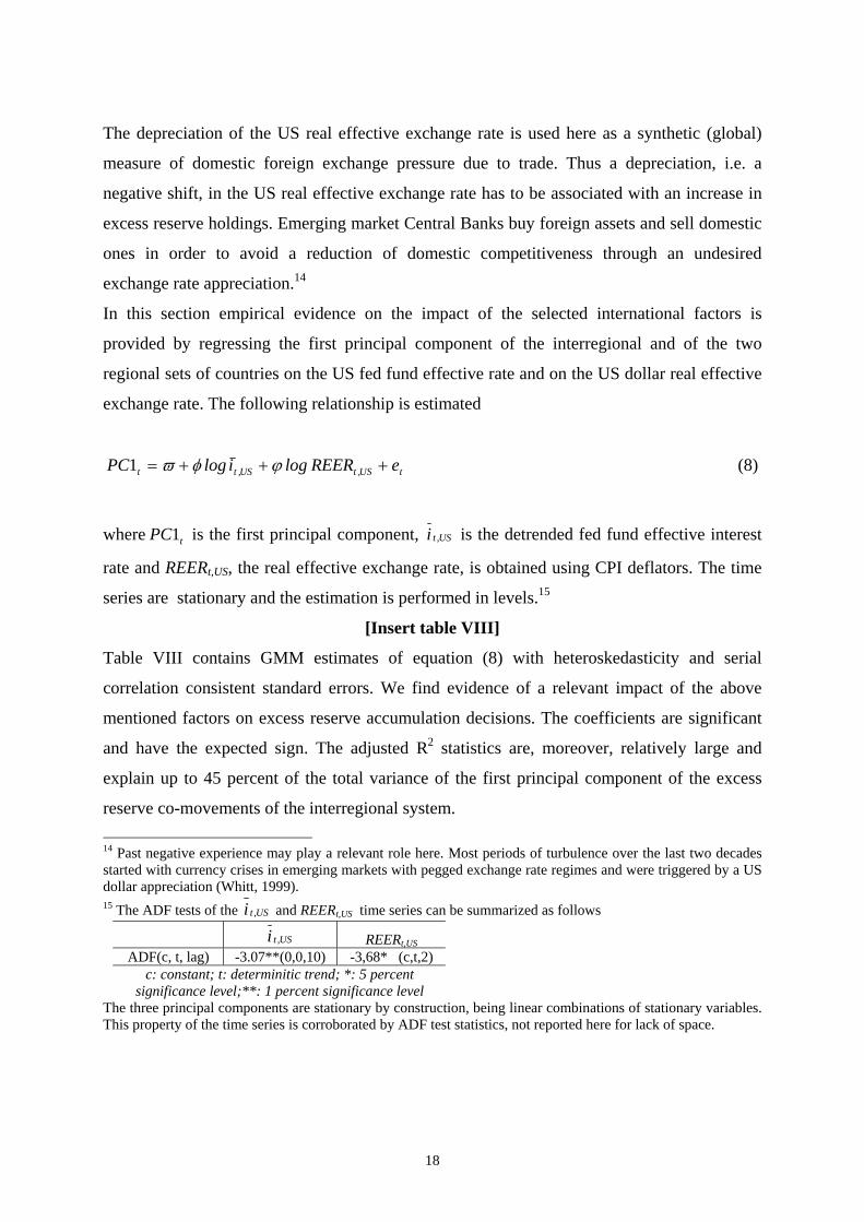
PC i REER et t US t U1 = + S t+ +ϖ φ ϕlog log, , (8)

where is the first principal component, PC t1 USti , is the detrended fed fund effective interest

rate and REERt,US, the real effective exchange rate, is obtained using CPI deflators. The time

series are stationary and the estimation is performed in levels.15

[Insert table VIII]

Table VIII contains GMM estimates of equation (8) with heteroskedasticity and serial

correlation consistent standard errors. We find evidence of a relevant impact of the above

mentioned factors on excess reserve accumulation decisions. The coefficients are significant

and have the expected sign. The adjusted R2 statistics are, moreover, relatively large and

explain up to 45 percent of the total variance of the first principal component of the excess

reserve co-movements of the interregional system. 14 Past negative experience may play a relevant role here. Most periods of turbulence over the last two decades started with currency crises in emerging markets with pegged exchange rate regimes and were triggered by a US dollar appreciation (Whitt, 1999). 15 The ADF tests of the USti , and REERt,US time series can be summarized as follows

USti , REERt,US

ADF(c, t, lag) -3.07**(0,0,10) -3,68* (c,t,2) c: constant; t: determinitic trend; *: 5 percent

significance level;**: 1 percent significance level The three principal components are stationary by construction, being linear combinations of stationary variables. This property of the time series is corroborated by ADF test statistics, not reported here for lack of space.

18

4 Conclusion

Large-scale accumulation of foreign reserves by emerging market economies has recently

attracted considerable attention. Most rules of thumb point out that reserve demand is

excessive with respect to common adequacy levels. These rules, however, are simplistic by

construction and tend to underestimate actual reserve requirements. This paper proposes an

alternative assessment of reserve adequacy based on long run estimates of the buffer stock

model for ten emerging countries, located in Asia and Latin America, over the 1985-2004

time period. Optimal reserves are the fitted values of cointegration relationships obtained with

the Johansen procedure and the corresponding cointegration residuals quantify excess reserve

holdings. Our results suggest that the current size of excess reserves is probably overstated in

the literature.

Over-accumulation may be attributed to Governments’ “fear of floating” and/or to a

mercantilist rationale. In the first case foreign reserves are stocked to reduce vulnerability to

external shocks in countries with uncertain and pro-cyclical access to global financial

markets. Capacity to draw on reserves smoothes consumption in the presence of external

shocks and reduces vulnerability to creditor runs arising from currency and maturity

mismatches. Mercantilist reserve accumulation is driven by a desire to maintain competitive

exchange rates and, hence, economic growth. (The thesis by Dooley et al. 2003 assumes that a

strategy of deliberately under-valuing the exchange rate to promote exports can deliver long

run benefits.) The relevance of these interpretations is corroborated by our empirical findings.

Cointegration residual co-movements - filtered using principal components analysis - are

investigated to detect the impact of common international factors such as the US fed fund rate

and the US dollar real effective exchange rate. The former represents the US monetary policy

and is an identified driver of international capital flows, while the latter quantifies adverse

external shocks on emerging markets competitiveness.

The US interest rate exerts a significant positive effect on excess reserve demand as central

bankers try to reduce their exposure to sudden capital reversals. In the same way, a

depreciation of the US dollar real effective exchange rate brings about an increase in excess

19

demand as central bankers react to the negative impact on competitiveness of an appreciation

of the domestic currency.

Central bankers' behavior is far from irrational and is explained by idiosyncratic and common

economic factors. Reserves are accumulated above buffer stock precautionary levels in order

to weather financial crises and to foster export led economic growth.

Bibliography

Aizenman, J., Marion, N., 2004. International Reserve Holdings with Sovereign Risk and

Costly Tax Collection. Economic Journal 114, 569-591.

Aizenman, J., Lee, Y., Rhee, Y., 2004. International Reserve Management and Capital

Mobility in a Volatile World: Policy Considerations and a Case Study of Korea.

NBER Working Paper Series n. 10534.

Aizenman, J., Lee, J., 2005. International Reserves: Precautionary versus Mercantilist Views,

Theory and Evidence. NBER Working Paper Series n. 11366.

Aportela, F., Gallego, F., García, P., 2005. Reserves over the Transitions to Floating: Lessons

from the Developed World. Mimeo, Central Bank of Chile.

Arora,V., Cerisola, M., 2001. How Does the US Monetary Policy Influence Sovereign Spread

in Emerging Markets? IMF Staff Papers 48, 474-498.

Bahmani-Oskooee, M., Brown, F., 2002. Demand for International Reserves: A Review

Article. Applied Economics 34, 1209-1226.

Bird, G., Rajan, R., 2002. Too Much of a Good Thing? The Adequacy of International

Reserves in the Aftermath of the Crises. Discussion Paper no.0210, CEIS Adelaide

University, Australia.

Boswijk, H.P., Lucas, A., Taylor, N., 2000. A Comparison of Parametric, Semi-

nonparametric, Adaptive and Nonparametric Cointegration Tests. Fomby, T.B., Hill,

R.C. (eds). Applying Kernel and Nonparametric Estimation to Economic Topics. JAI

Press, Stamford.

Bussière, M., Mulder, C., 1999. External Vulnerability in Emerging Market Economies: How

High Liquidity Can Offset Weak Fundamentals and the Effects of Contagion. IMF

Working Paper 99/88.

20

Calvo, G., Leiderman, L., Reinhart, C., 1996. Inflows of Capital to Developing Countries in

the 1990’s. Journal of Economic Perspectives 10, 123-139.

Calvo, G., Reinhart, C., 2002. Fear of Floating. Quarterly Journal of Economics, 2, 379-408.

De Beaufort Wijnholds, J.O., Kapteyn, A., 2001. Reserve Adequacy in Emerging Market

Economies. IMF Working Paper 01/43.

Dooley, M.P., Folkerts-Landau, D., Garber, P., 2003. An Essay on the Revised Bretton

Woods System. NBER Working Paper Series n. 9971.

Edwards, S., 1985. On the Interest-Rate Elasticity of the Demand for International Reserves:

Some Evidence from Developing Countries. Journal of International Money and

Finance 4, 287-295.

Flood, R., Marion, N., 2002. Holding International Reserves in an Era of High Capital

Mobility. IMF Working Paper 02/62.

Frankel, J., 1999. No Single Currency Regime is Right for All Countries or at All Times.

NBER Working Paper Series, n. 7338.

Franses, P.H., Haldrup, N., 1994. The Effect of Additive Outliers on Tests for Unit Roots and

Cointegration. Journal of Business and Economic Statistics 12, 471-478.

Frenkel, J.A., 1974. The Demand for International Reserves by Developed and Less

Developed Countries. Economica 41, 14-24.

Frenkel, J.A., Jovanovic, B., 1981. Optimal International Reserves: A Stochastic Framework.

Economic Journal 91, 507-514.

Glosten, L.R., Jagannathan, R., Runkle, D., 1993. On the Relation Between the Expected

Value and the Volatility of the Nominal Excess Return on Stocks. Journal of Finance

48, 1779-1801.

Hamada, K., Ueda, K., 1977. Random Walks and the Theory of the Optimal International

Reserves. Economic Journal 87, 722-742.

Heller, R.H., 1966. Optimal International Reserves. Economic Journal 76, 296-311.

Heller, R.H., 1968. The Transaction Demand for International Means of Payment. Journal of

Political Economy 76, 141-145.

Hendry, D.F., Doornik, J.A., 1994. Modelling Linear Dynamic Econometric Models. Scottish

Journal of Political Economy 41, 1-33.

21

International Monetary Fund, 1958. International Reserves and Liquidity, A Study by the

Staff of the International Monetary Fund. Washington DC.

International Monetary Fund, 2000. Debt- and Reserve-Related Indicators of External

Vulnerability. Policy Development and Review Department, Washington DC.

Available at http://www.imf.org/external/np/pdr/debtres/index.htm

Johansen, S., 1988. Statistical Analysis of Cointegration Vectors. Journal of Economic

Dynamics and Control 12, 231-254.

Johansen, S., 1991. Estimation and Hypothesis Testing of Cointegration Vectors in Gaussian

Vector Autoregressive Models. Econometrica 59, 1551-1580.

Johansen, S., 1995. Likelihood-Based Inference in Cointegrated Vector Autoregressive

Models. Oxford University Press, Oxford.

Johansen, S., Juselius, K., 1990. Maximum Likelihood estimation and Inference on

Cointegration – with Applications to the Demand for Money. Oxford Bulletin of

Economics and Statistics 52, 169-210.

Kaminsky, G., Lizondo, S., Reinhart, C., 1997. Leading Indicators of Currency Crises. Policy

Research Working Paper n. 1852, World Bank.

Mody, A., Taylor, M., Kim, J.Y., 2001. Forecasting Capital Flows to Emerging Markets: a

Kalman Filtering Approach. Applied Financial Economics 11, 581-589.

Nelson, D., 1990. Stationarity and Persistence in the GARCH(1,1) Model. Econometric

Theory 6, 318-334.

Ng, S., Perron, P., 2001. Lag Length Selection and the Construction of Unit Root Tests with

Good Size and Power. Econometrica 69, 1519-1554.

Nielsen, H.B., 2004. Cointegration Analysis in the Presence of Outliers. Econometrics Journal

7, 249-271.

Perron, P., Rodríguez, G., 2003. Searching for Additive Outliers in Nonstationary Time

Series. Journal of Time Series Analysis 24, 193-220.

Triffin, R., 1960. Gold and the Dollar Crisis. Yale University Press, New Haven.

Uribe, M., Yue, V.Z., 2003. Country Spreads and Emerging Countries: Who Drives Whom?

NBER Working Paper Series n.10018.

Vogelsang, T.J., 1999. Two Simple Procedures for Testing for a Unit Root When There Are

Additive Outliers. Journal of Time Series Analysis 20, 237-252.

22

Whitt, J., 1999. The Role of External Shocks in Asian Financial Crises. Economic Review

Federal Reserve Bank of Atlanta, Second Quarter 18-31.

APPENDIX I

Data description

Time series are monthly and cover the period between January 1985 and December 2004.

- Reserves excluding gold are series l1da quoted in US dollars from the IMF International Financial

Statistics Data Base. International reserves do not include gold because of valuation problems and of

the modest amount of the precious metal in the EME reserve stocks.

- Interest rates are the money market rates in series 60b for Argentina, Brazil, Indonesia, Korea,

Malaysia, Mexico, and Singapore. Treasury bill rate in series 60c was used for the Philippines. The

deposit rate in series 60l was used for Chile and Venezuela. They are all from the IMF International

Financial Statistics Data Base.

- Imports are series 71da (cif quoted in US dollars) from the IMF International Financial Statistics Data

Base.

- M2 is the sum of M1 series 35a and Quasi money 34a. The M2 series are quoted in national currency

and were converted into US dollars using the end of period exchange rate. They are all obtained from

the IMF International Financial Statistics Data Base.

- Real effective exchange rate for the US is USI..RECE - CPI BASED SADJ from the IMF

International Financial Statistics Data Base.

- US short interest rate, federal fund effective interest rate is from the Federal Reserve database.

- Short term external debt series are taken from the IIF data base but for the Singaporean one which is

computed adding item G-H-I taken from the BIS/IMF/World Bank /OECD data base.

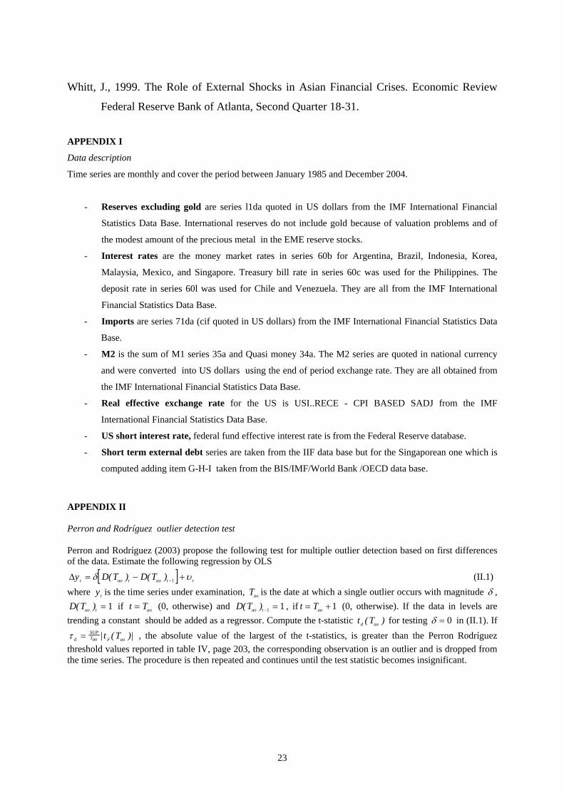
APPENDIX II Perron and Rodríguez outlier detection test Perron and Rodríguez (2003) propose the following test for multiple outlier detection based on first differences of the data. Estimate the following regression by OLS

[∆y D T D Tt ao t ao t= − −δ ( ) ( ) 1 ] t+υ (II.1) where is the time series under examination, is the date at which a single outlier occurs with magnitude yt Tao δ ,

if (0, otherwise) and D Tao t( ) = 1 t Tao= D Tao t( ) − =1 1 , if t Tao= +1 (0, otherwise). If the data in levels are trending a constant should be added as a regressor. Compute the t-statistic t T for testing d ao( ) δ = 0 in (II.1). If τ δd

SUPTao aot T= | ( )| , the absolute value of the largest of the t-statistics, is greater than the Perron Rodríguez

threshold values reported in table IV, page 203, the corresponding observation is an outlier and is dropped from the time series. The procedure is then repeated and continues until the test statistic becomes insignificant.

23

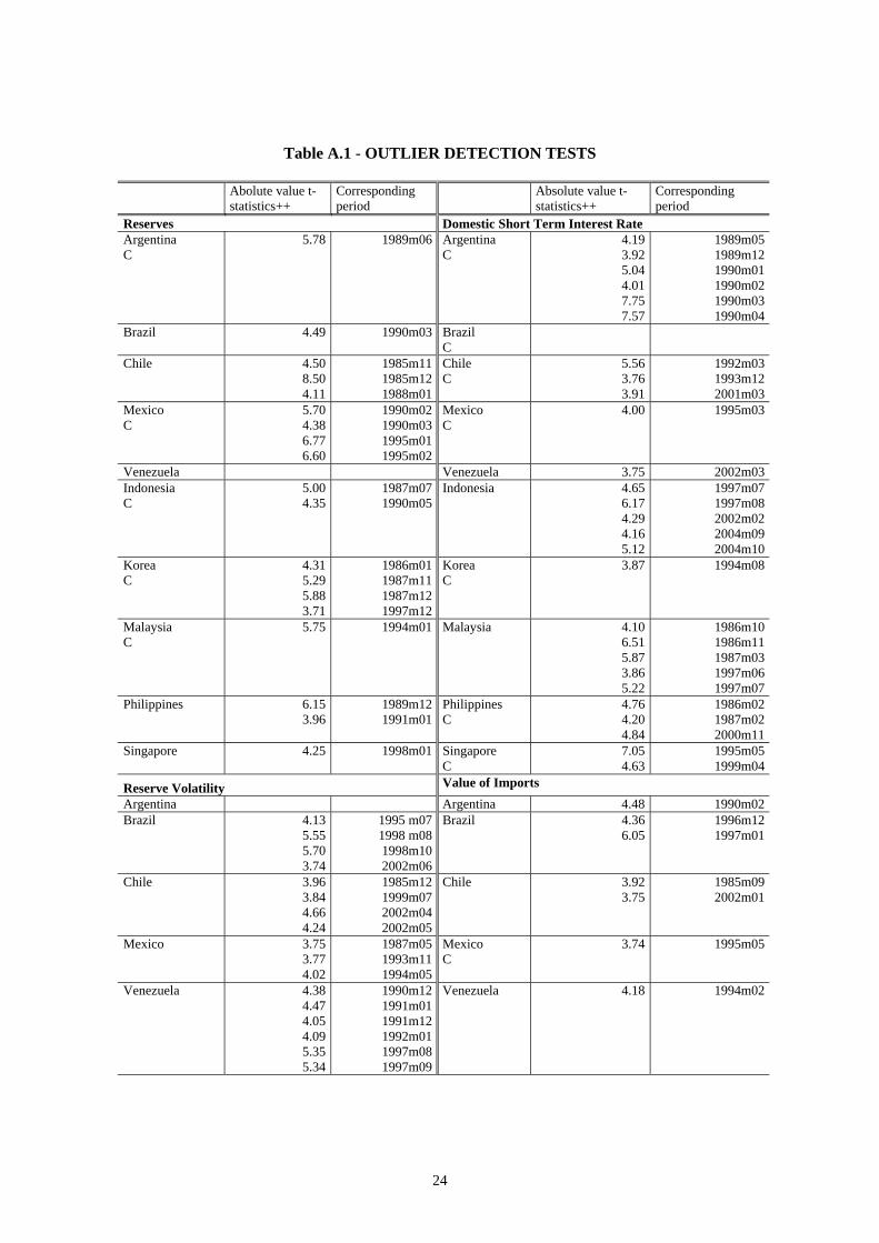
Table A.1 - OUTLIER DETECTION TESTS

Abolute value t- statistics++

Corresponding period

Absolute value t- statistics++

Corresponding period

Reserves Domestic Short Term Interest Rate Argentina C

5.78 1989m06 Argentina C

4.19 3.92 5.04 4.01 7.75 7.57

1989m051989m121990m011990m021990m031990m04

Brazil

4.49 1990m03 Brazil C

Chile

4.50 8.50 4.11

1985m111985m121988m01

Chile C

5.56 3.76 3.91

1992m031993m122001m03

Mexico C

5.70 4.38 6.77 6.60

1990m021990m031995m011995m02

Mexico C

4.00 1995m03

Venezuela Venezuela 3.75 2002m03Indonesia C

5.00 4.35

1987m071990m05

Indonesia

4.65 6.17 4.29 4.16 5.12

1997m071997m082002m022004m092004m10

Korea C

4.31 5.29 5.88 3.71

1986m011987m111987m121997m12

Korea C

3.87 1994m08

Malaysia C

5.75 1994m01 Malaysia

4.10 6.51 5.87 3.86 5.22

1986m101986m111987m031997m061997m07

Philippines 6.15 3.96

1989m121991m01

Philippines C

4.76 4.20 4.84

1986m021987m022000m11

Singapore 4.25 1998m01 Singapore C

7.05 4.63

1995m051999m04

Reserve Volatility Value of Imports Argentina Argentina 4.48 1990m02Brazil 4.13

5.55 5.70 3.74

1995 m071998 m081998m102002m06

Brazil 4.36 6.05

1996m121997m01

Chile

3.96 3.84 4.66 4.24

1985m121999m072002m042002m05

Chile 3.92 3.75

1985m092002m01

Mexico

3.75 3.77 4.02

1987m051993m111994m05

Mexico C

3.74 1995m05

Venezuela

4.38 4.47 4.05 4.09 5.35 5.34

1990m121991m011991m121992m011997m081997m09

Venezuela

4.18 1994m02

24

Indonesia 4.38 2000m08 Indonesia C

3.86 4.53

1986m121990m04

Korea C

4.77 3.88 3.99 3.94

1997m111997m122003m052003m06

Korea C

4.00 5.19 4.46

1985m121986m121987m01

Malaysia

3.81 4.23 5.31 4.93

1990m101990m111992m081992m09

Malaysia

3.79 1997m02

Philippines 4.74 3.76 4.20 3.95

1997m071997m082000m032000m04

Philippines

3.97 1998m05

Singapore C

4.97 1995m03 Singapore C

4.26 4.99 4.06

1997m021998m041998m05

Notes. ++ : Perron and Rodríguez (2003) critical values with constant: 4.20(1%), 3.75 (5%), 3.56 (10%); with constant and trend: 4.19(1%), 3.74 (5%), 3.55 (10%); C: constant term in equation (II.1).

APPENDIX III Analysis of the conditional heteroskedasticity of the international reserves first difference time series

Table A.II - CONDITIONAL HETEROSKEDASTICITY TESTS

LB Q(j)

Argentina

Brazil

Chile

Mexico

Venezuela

Indonesia

Korea

Malaysia

Philippines

Singapore

3 63.91**

0.34

5.61*

20.63**

6.39*

33.11**

27.95**

36.07**

5.11*

52.08**

5 71.50**

6.41

8.68*

33.23**

8.12*

39.30**

35.00**

36.73**

18.05**

91.76**

7 83.22**

22.53**

11.19*

40.54**

8.97

39.76**

43.91**

37.86**

19.51**

135.56**

Notes. LB Q(j): Ljung Box Q-statistic for the null of no autocorrelation up to order j; *: rejected at the 5% level; **: rejected at the 1% level. The reserve first differences have been filtered, if necessary, in order to eliminate serial correlation. The number of degrees of freedom of the χ2 distribution has been correspondingly adjusted.

25

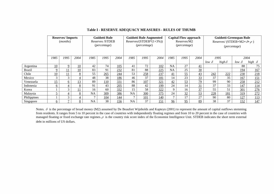
Table I - RESERVE ADEQUACY MEASURES - RULES OF THUMB

Reserves/ Imports

(months) Guidotti Rule

Reserves /STDEB (percentage)

Guidotti Rule Augmented Reserves/(STDEB*(1+3%))

(percentage)

Capital Flow approach Reserves/M2 (percentage)

Guidotti-Greenspan Rule ∗ ∗ Reserves/ (STDEB+M2 δ ρ )

(percentage)

1985 1995 2004 1985 1995 2004 1985 1995 2004 1985 1995 2004 1995low δ highδ

2004 low δ high δ

Argentina 10 9 10 42 74 105 41 72 102 NA 27 41 88 75Brazil 9 11 10 83 91 232 81 88 225 NA 25 30 194 167Chile 10 11 8 55 265 244 53 258 237 41 55 43 242 222 230 218Mexico 3 3 4 48 38 186 46 37 181 14 23 33 37 35 167 151Venezuela 15 6 13 89 110 331 86 107 321 42 53 79 99 90 258 212Indonesia 6 4 8 91 43 205 88 42 199 24 14 31 37 33 147 114Korea 1 3 11 16 60 332 15 58 322 9 16 37 55 51 301 276Malaysia 5 4 8 NA 309 386 NA 300 375 24 32 53 228 181 319 272Philippines 1 3 4 7 104 144 7 101 140 7 17 27 90 80 127 113Singapore 6 7 8 NA 38 156 NA 37 151 96 95 89 38 37 152 147

Notes. δ is the percentage of broad money (M2) assumed by De Beaufort Wijnholds and Kapteyn (2001) to represent the amount of capital outflows stemming from residents. It ranges from 5 to 10 percent in the case of countries with independently floating regimes and from 10 to 20 percent in the case of countries with managed floating or fixed exchange rate regimes. ρ is the country risk score index of the Economist Intelligence Unit. STDEB indicates the short term external debt in millions of US dollars.

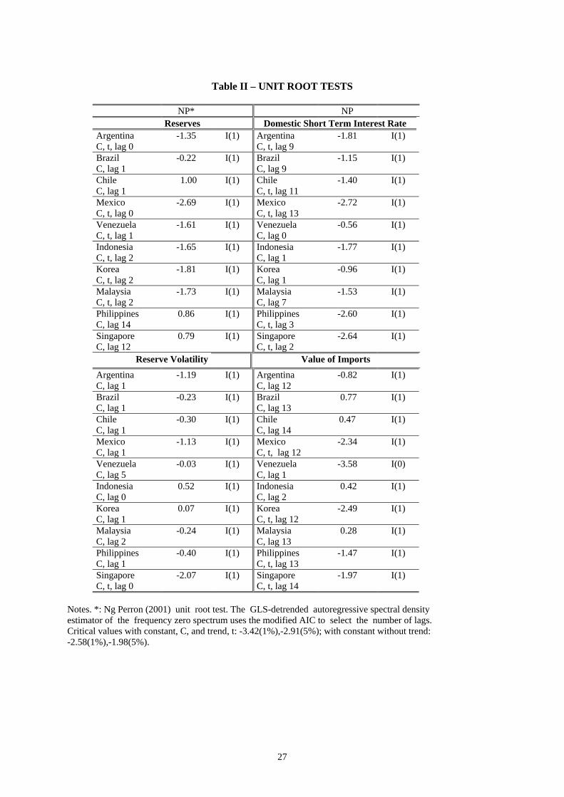
Table II – UNIT ROOT TESTS

NP* NP Reserves Domestic Short Term Interest Rate

Argentina C, t, lag 0

-1.35 I(1) Argentina C, t, lag 9

-1.81 I(1)

Brazil C, lag 1

-0.22 I(1) Brazil C, lag 9

-1.15 I(1)

Chile C, lag 1

1.00 I(1) Chile C, t, lag 11

-1.40 I(1)

Mexico C, t, lag 0

-2.69 I(1) Mexico C, t, lag 13

-2.72 I(1)

Venezuela C, t, lag 1

-1.61 I(1) Venezuela C, lag 0

-0.56 I(1)

Indonesia C, t, lag 2

-1.65 I(1) Indonesia C, lag 1

-1.77 I(1)

Korea C, t, lag 2

-1.81 I(1) Korea C, lag 1

-0.96 I(1)

Malaysia C, t, lag 2

-1.73 I(1) Malaysia C, lag 7

-1.53 I(1)

Philippines C, lag 14

0.86 I(1) Philippines C, t, lag 3

-2.60 I(1)

Singapore C, lag 12

0.79 I(1) Singapore C, t, lag 2

-2.64 I(1)

Reserve Volatility Value of Imports

Argentina C, lag 1

-1.19 I(1) Argentina C, lag 12

-0.82 I(1)

Brazil C, lag 1

-0.23 I(1) Brazil C, lag 13

0.77 I(1)

Chile C, lag 1

-0.30 I(1) Chile C, lag 14

0.47 I(1)

Mexico C, lag 1

-1.13 I(1) Mexico C, t, lag 12

-2.34 I(1)

Venezuela C, lag 5

-0.03 I(1) Venezuela C, lag 1

-3.58 I(0)

Indonesia C, lag 0

0.52 I(1) Indonesia C, lag 2

0.42 I(1)

Korea C, lag 1

0.07 I(1) Korea C, t, lag 12

-2.49 I(1)

Malaysia C, lag 2

-0.24 I(1) Malaysia C, lag 13

0.28 I(1)

Philippines C, lag 1

-0.40 I(1) Philippines C, t, lag 13

-1.47 I(1)

Singapore C, t, lag 0

-2.07

I(1) Singapore C, t, lag 14

-1.97 I(1)

Notes. *: Ng Perron (2001) unit root test. The GLS-detrended autoregressive spectral density estimator of the frequency zero spectrum uses the modified AIC to select the number of lags. Critical values with constant, C, and trend, t: -3.42(1%),-2.91(5%); with constant without trend: -2.58(1%),-1.98(5%).

27

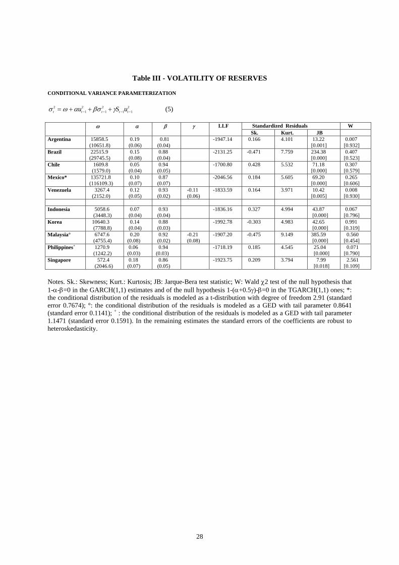
Table III - VOLATILITY OF RESERVES

CONDITIONAL VARIANCE PARAMETERIZATION σ ω α βσ γt t t tu S2

12

12

1 12= + + +− − − tu − (5)

ω α β γ LLF Standardized Residuals W Sk. Kurt. JB Argentina 15858.5

(10651.8) 0.19 (0.06)

0.81 (0.04)

-1947.14 0.166 4.101 13.22 [0.001]

0.007 [0.932]

Brazil 22515.9 (29745.5)

0.15 (0.08)

0.88 (0.04)

-2131.25 -0.471 7.759 234.38 [0.000]

0.407 [0.523]

Chile 1609.8 (1579.0)

0.05 (0.04)

0.94 (0.05)

-1700.80 0.428 5.532 71.18 [0.000]

0.307 [0.579]

Mexico* 135721.8 (116109.3)

0.10 (0.07)

0.87 (0.07)

-2046.56 0.184 5.605 69.20 [0.000]

0.265 [0.606]

Venezuela 3267.4 (2152.0)

0.12 (0.05)

0.93 (0.02)

-0.11 (0.06)

-1833.59 0.164 3.971 10.42 [0.005]

0.008 [0.930]

Indonesia 5058.6

(3448.3) 0.07 (0.04)

0.93 (0.04)

-1836.16 0.327 4.994 43.87 [0.000]

0.067 [0.796]

Korea 10640.3 (7788.8)

0.14 (0.04)

0.88 (0.03)

-1992.78 -0.303 4.983 42.65 [0.000]

0.991 [0.319]

Malaysia° 6747.6 (4755.4)

0.20 (0.08)

0.92 (0.02)

-0.21 (0.08)

-1907.20 -0.475 9.149 385.59 [0.000]

0.560 [0.454]

Philippines+ 1270.9 (1242.2)

0.06 (0.03)

0.94 (0.03)

-1718.19 0.185 4.545 25.04 [0.000]

0.071 [0.790]

Singapore 572.4 (2046.6)

0.18 (0.07)

0.86 (0.05)

-1923.75 0.209 3.794 7.99 [0.018]

2.561 [0.109]

Notes. Sk.: Skewness; Kurt.: Kurtosis; JB: Jarque-Bera test statistic; W: Wald χ2 test of the null hypothesis that 1-α-β=0 in the GARCH(1,1) estimates and of the null hypothesis 1-(α+0.5γ)-β=0 in the TGARCH(1,1) ones; *: the conditional distribution of the residuals is modeled as a t-distribution with degree of freedom 2.91 (standard error 0.7674); °: the conditional distribution of the residuals is modeled as a GED with tail parameter 0.8641 (standard error 0.1141); + : the conditional distribution of the residuals is modeled as a GED with tail parameter 1.1471 (standard error 0.1591). In the remaining estimates the standard errors of the coefficients are robust to heteroskedasticity.

28

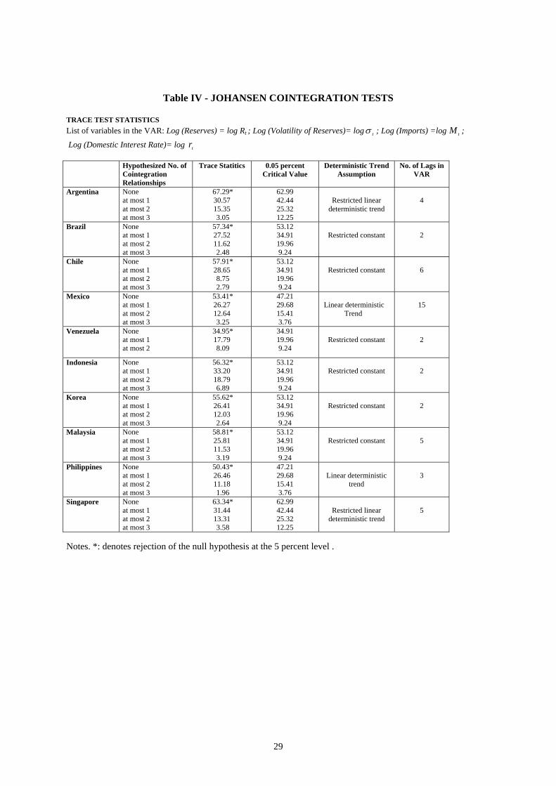
Table IV - JOHANSEN COINTEGRATION TESTS

TRACE TEST STATISTICS List of variables in the VAR: Log (Reserves) = log Rt ; Log (Volatility of Reserves)= logσ t ; Log (Imports) =log ; M t

Log (Domestic Interest Rate)= log r t

Hypothesized No. of

Cointegration Relationships

Trace Statitics 0.05 percent Critical Value

Deterministic Trend Assumption

No. of Lags in VAR

Argentina None at most 1 at most 2 at most 3

67.29* 30.57 15.35 3.05

62.99 42.44 25.32 12.25

Restricted linear

deterministic trend

4

Brazil None at most 1 at most 2 at most 3

57.34* 27.52 11.62 2.48

53.12 34.91 19.96 9.24

Restricted constant

2

Chile None at most 1 at most 2 at most 3

57.91* 28.65 8.75 2.79

53.12 34.91 19.96 9.24

Restricted constant

6

Mexico None at most 1 at most 2 at most 3

53.41* 26.27 12.64 3.25

47.21 29.68 15.41 3.76

Linear deterministic Trend

15

Venezuela None at most 1 at most 2

34.95* 17.79 8.09

34.91 19.96 9.24

Restricted constant

2

Indonesia None at most 1 at most 2 at most 3

56.32* 33.20 18.79 6.89

53.12 34.91 19.96 9.24

Restricted constant

2

Korea None at most 1 at most 2 at most 3

55.62* 26.41 12.03 2.64

53.12 34.91 19.96 9.24

Restricted constant

2

Malaysia None at most 1 at most 2 at most 3

58.81* 25.81 11.53 3.19

53.12 34.91 19.96 9.24

Restricted constant

5

Philippines None at most 1 at most 2 at most 3

50.43* 26.46 11.18 1.96

47.21 29.68 15.41 3.76

Linear deterministic

trend

3

Singapore None at most 1 at most 2 at most 3

63.34* 31.44 13.31 3.58

62.99 42.44 25.32 12.25

Restricted linear

deterministic trend

5

Notes. *: denotes rejection of the null hypothesis at the 5 percent level .

29

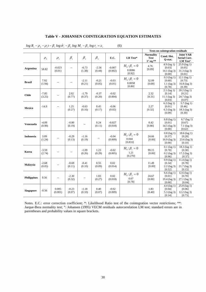
Table V - JOHANSEN COINTEGRATION EQUATION ESTIMATES

(6) log log $ log logR t M rt t t t t− − − − − =ρ ρ β σ β β ε0 1 2 3 t

Tests on cointegration residuals

ρ0 ρ1 β1 β2 β3

E.C.

LR Test* Normality

Test 1° eq.**

Cond. Het. Q-stat.

Joint VAR Serial Corr.

LM Test°

Argentina 58.82 -0.023 (0.01)

--

-6.73 (1.38)

-2.56 (0.44)

-0.007 (0.002)

H0 1 0:β = 0.0086 [0.92]

4.76 [0.09]

4.9 (lag 1) [0.03]

14.1 (lag 3) [0.00]

25.9 (lag 1) [0.05] 31.3 (lag 3)

[0.01]

Brazil 7.92 (1.94) -- -- -2.11

(0.21) -0.21 (0.05)

-0.03 (0.01)

H0 1 0:β = 0.0058 [0.80]

32.09 [0.00]

0.3 (lag 1)[0.60]

1.1 (lag 3)[0.78]

12.1 (lag 1) [0.73] 16.8 (lag 3) [0.39]

Chile -7.85 (3.25) -- 2.02

(0.77) -1.79 (0.37)

-0.37 (0.20)

-0.02 (0.004) 2.32

[0.31]

2.1 (lag 1) [0.14] 11.1 (lag 3) [0.03]

20.2 (lag 1) [0.21] 24.7 (lag 3)

[0.07]

Mexico

-14.9

--

1.25 (0.27)

-0.63 (0.16)

0.45 (0.17)

-0.06 (0.02)

2.27 [0.32]

6.2 (lag 1) [0.01] 6.3 (lag 3)

[0.09]

5.7 (lag 1) [0.46] 18.3 (lag 3) [0.30]

Venezuela -4.09 (0.99) -0.80

(0.19) -- 0.24 (0.11)

-0.027 (0.018) 0.42

[0.80]

6.8 (lag 1)[0.01]

14.5 (lag 3)[0.00]

6.7 (lag 1) [0.67] 7.1 (lag 3) [0.62]

Indonesia

3.09 (1.24)

-- -0.29 (0.13)

-1.16 (0.19)

-- -0.04 (0.009)

H0 3 0:β = 0.044 [0.833]

24.66 [0.00]

0.8 (lag 1)[0.37]

16.9 (lag 3)[0.00]

18.6 (lag 1) [0.28]

23.6 (lag 3)[0.10]

Korea -3.59 (2.74) -- -- -1.09

(0.26) 1.23

(0.29) -0.02

(0.005)

H0 1 0:β = 1.21

[0.270]

99.15 [0.00]

0.1 (lag 1)[0.70]

0.2 (lag 3)[0.96]

18.3 (lag 1) [0.30]

17.2 (lag 3) [0.37]

Malaysia -2.68 (0.05) -- -0.69

(0.11) -0.41 (0.10)

0.55 (0.09)

0.02 (0.014) 11.49

[0.00]

0.9 (lag 1)[0.34]

2.2 (lag 3)[0.52]

11.4 (lag 1) [0.78]

21.7 (lag 3) [0.15]

Philippines 0.56 -- -2.30 (0.32) -- 1.83

(0.27) 0.02

(0.018)

H0 2 0:β = 0.07

[0.78]

24.67 [0.00]

6.6 (lag 1)[0.01]

19.4 (lag 3)[0.00]

12.6 (lag 1) [0.70]

27.1 (lag 3) [0.04]

Singapore -0.56 0.005 (0.001)

-0.23 (0.07)

-1.18 (0.10)

0.40 (0.07)

-0.02 (0.009) 1.83

[0.40]

4.4 (lag 1)[0.04]

5.3 (lag 3)[0.14]

25.8 (lag 1) [0.06]

12.2 (lag 3) [0.73]

Notes. E.C.: error correction coefficient; *: Likelihood Ratio test of the cointegration vector restrictions; **: Jarque-Bera normality test; °: Johansen (1995) VECM residuals autocorrelation LM test; standard errors are in parentheses and probability values in square brackets.

30

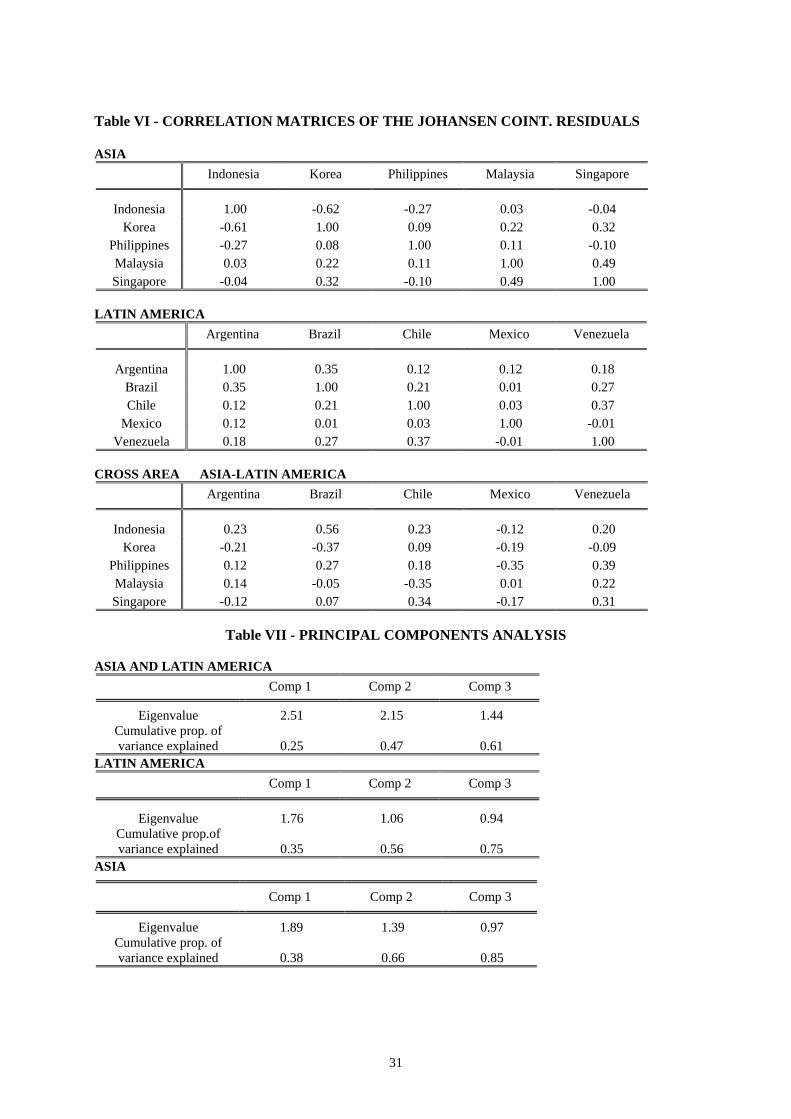
Table VI - CORRELATION MATRICES OF THE JOHANSEN COINT. RESIDUALS ASIA

Indonesia Korea Philippines Malaysia Singapore

Indonesia 1.00 -0.62 -0.27 0.03 -0.04 Korea -0.61 1.00 0.09 0.22 0.32

Philippines -0.27 0.08 1.00 0.11 -0.10 Malaysia 0.03 0.22 0.11 1.00 0.49 Singapore -0.04 0.32 -0.10 0.49 1.00

LATIN AMERICA

Argentina Brazil Chile Mexico Venezuela

Argentina 1.00 0.35 0.12 0.12 0.18 Brazil 0.35 1.00 0.21 0.01 0.27 Chile 0.12 0.21 1.00 0.03 0.37

Mexico 0.12 0.01 0.03 1.00 -0.01 Venezuela 0.18 0.27 0.37 -0.01 1.00

CROSS AREA ASIA-LATIN AMERICA

Argentina Brazil Chile Mexico Venezuela

Indonesia 0.23 0.56 0.23 -0.12 0.20 Korea -0.21 -0.37 0.09 -0.19 -0.09

Philippines 0.12 0.27 0.18 -0.35 0.39 Malaysia 0.14 -0.05 -0.35 0.01 0.22 Singapore -0.12 0.07 0.34 -0.17 0.31

Table VII - PRINCIPAL COMPONENTS ANALYSIS

ASIA AND LATIN AMERICA

Comp 1 Comp 2 Comp 3

Eigenvalue 2.51 2.15 1.44 Cumulative prop. of variance explained 0.25 0.47 0.61

LATIN AMERICA Comp 1 Comp 2 Comp 3

Eigenvalue 1.76 1.06 0.94 Cumulative prop.of variance explained 0.35 0.56 0.75

ASIA

Comp 1 Comp 2 Comp 3

Eigenvalue 1.89 1.39 0.97 Cumulative prop. of variance explained 0.38 0.66 0.85

31

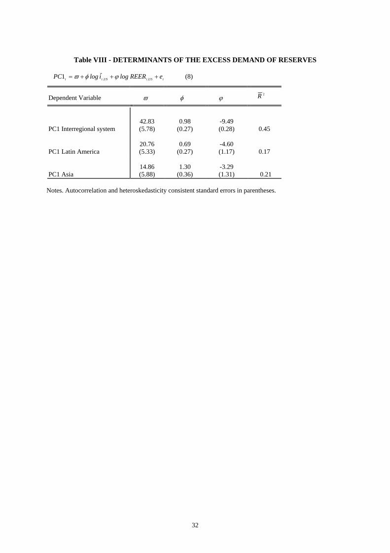
Table VIII - DETERMINANTS OF THE EXCESS DEMAND OF RESERVES

PC i REER et t US t US, t1 = + + +ϖ φ ϕlog log, (8)

Dependent Variable ϖ φ ϕ R 2

PC1 Interregional system 42.83 (5.78)

0.98 (0.27)

-9.49 (0.28) 0.45

PC1 Latin America 20.76 (5.33)

0.69 (0.27)

-4.60 (1.17) 0.17

PC1 Asia 14.86 (5.88)

1.30 (0.36)

-3.29 (1.31) 0.21

Notes. Autocorrelation and heteroskedasticity consistent standard errors in parentheses.

32

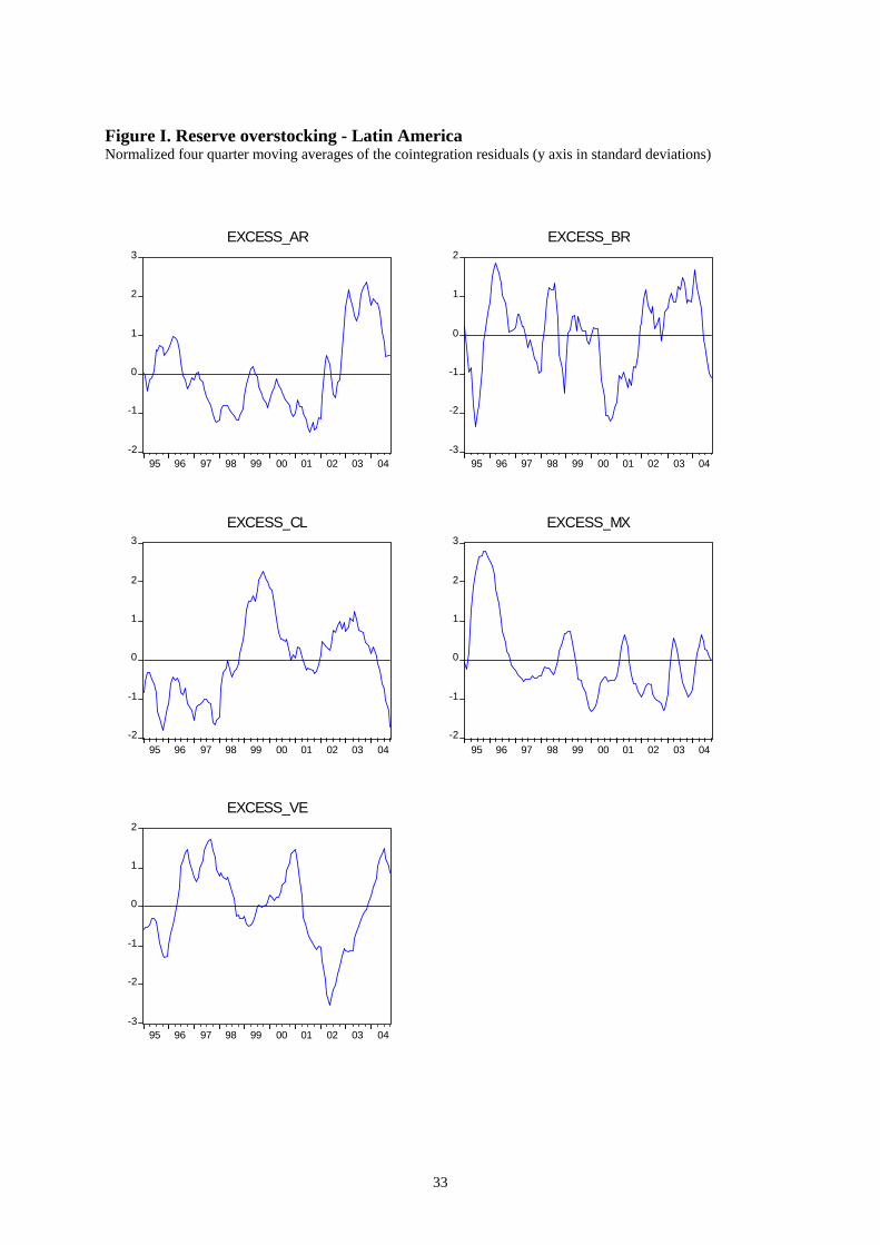
Figure I. Reserve overstocking - Latin America Normalized four quarter moving averages of the cointegration residuals (y axis in standard deviations)

-2.0

-1.5

-1.0

-0.5

0.0

0.5

1.0

1.5

2.0

95 96 97 98 99 00 01 02 03 04

EXCESS_ID

-2

-1

0

1

2

3

4

95 96 97 98 99 00 01 02 03 04

EXCESS_KO

-2

-1

0

1

2

3

95 96 97 98 99 00 01 02 03 04

EXCESS_MY

-3

-2

-1

0

1

2

95 96 97 98 99 00 01 02 03 04

EXCESS_PH

-3

-2

-1

0

1

2

3

95 96 97 98 99 00 01 02 03 04

EXCESS_SP

-2

-1

0

1

2

3

95 96 97 98 99 00 01 02 03 04

EXCESS_AR

-3

-2

-1

0

1

2

95 96 97 98 99 00 01 02 03 04

EXCESS_BR

-2

-1

0

1

2

3

95 96 97 98 99 00 01 02 03 04

EXCESS_CL

-2

-1

0

1

2

3

95 96 97 98 99 00 01 02 03 04

EXCESS_MX

-3

-2

-1

0

1

2

95 96 97 98 99 00 01 02 03 04

EXCESS_VE

33

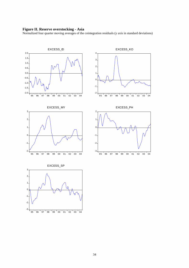
Figure II. Reserve overstocking - Asia Normalized four quarter moving averages of the cointegration residuals (y axis in standard deviations)

-2.0

-1.5

-1.0

-0.5

0.0

0.5

1.0

1.5

2.0

95 96 97 98 99 00 01 02 03 04

EXCESS_ID

-2

-1

0

1

2

3

4

95 96 97 98 99 00 01 02 03 04

EXCESS_KO

-2

-1

0

1

2

3

95 96 97 98 99 00 01 02 03 04

EXCESS_MY

-3

-2

-1

0

1

2

95 96 97 98 99 00 01 02 03 04

EXCESS_PH

-3

-2

-1

0

1

2

3

95 96 97 98 99 00 01 02 03 04

EXCESS_SP

34