Poverty and Social Dynamics Paper Series PSDPS : 1

Pakistan Panel Household Survey Sample Size, Attrition and

Socio-demographic Dynamics

Durr-e-Nayab

and

G. M. Arif

PAKISTAN INSTITUTE OF DEVELOPMENT ECONOMICS ISLAMABAD

All rights reserved. No part of this publication may be reproduced, stored in a retrieval system or transmitted in any form or by any means—electronic, mechanical, photocopying, recording or otherwise—without prior permission of the Publications Division, Pakistan Institute of Development Economics, P. O. Box 1091, Islamabad 44000.

© Pakistan Institute of Development Economics, 2012.

Pakistan Institute of Development Economics Islamabad, Pakistan E-mail: publications@pide.org.pk Website: http://www.pide.org.pk Fax: +92-51-9248065

Designed, composed, and finished at the Publications Division, PIDE.

C O N T E N T S

Page

1. Introduction and Background 1

2. Selection of Districts and Primary Sampling Units (PSUs) 2

3. Handling the Split Households 4

4. Sample Size Over the Different Rounds 5

5. Scope of the Panel Survey 6

6. An Analysis of the Sample Attrition 7

6.1. Theoretical Considerations 7

6.2. Extent of Attrition 9

6.3. Attrition Bias 9

7. Socio-demographic Profile of the Sample 12

7.1. Mean Household Size and Sex Ratio 12

7.2. Dependency Ratio 13

7.3. Age-sex Structure 14

7.4. Head of Households—Their Sex and Age 15

7.5. Marital Status 17

7.6. Literacy Rates 18

7.7. Employment 20

8. Conclusions 23

Annexures 24

References 28

List of Tables Table 1. Primary Sampling Units (PSUs) by Province and District 3

Table 2. Households Covered during the Three Waves of the Panel Survey 5

(iv)

Page

Table 3. Scope of the Panel Survey: Modules included in Household Questionnaires 7

Table 4. Sample Attrition Rates of Panel Households—Rural 9

Table 5. Determinants of Attrition through Logit Regression 10

Table 6. Household Expenditure: OLS Regression Model 2001-2010 11

Table 7. Correlates of Poverty: Logistic Regression Model 2001-2010 12

Table 8. Mean Household Size and Sex Ratio by Consumption Quintiles 13

Table 9. Dependency Ratio by Consumption Quintile 14

Table 10. Proportion of Female Headed Households and Mean Age of Household Heads by Sex 16

Table 11. Literacy Rates by Age, Sex and Consumption Quintiles (%) 19

List of Figures Figure 1. Map Showing Selected Districts for the PPHS-2010 4

Figure 2. Age-sex Pyramids 15

Figure 3. Proportion Never-Married by Age and Sex (%) 17

Figure 4. Crude and Refined Activity Rates (Age 10 Years and Above) by Sex and Region in PPHS-2010 21

Figure 5. Age Specific Activity Rates by Sex (%) 22

Figure 6. Unemployment Rate by Sex and Region (%) 22

1. INTRODUCTION AND BACKGROUND *

The socio-economic databases in Pakistan, as in most countries, can be classified into three broad categories, namely registration-based statistics, data produced by different population censuses and household survey-based data. The registration system of births and deaths in Pakistan has historically been inadequate [Afzal and Ahmed (1974)] and the population censuses have not been carried out regularly. The household surveys such as Pakistan Demographic Survey (PDS), Labour Force Survey (LFS) and Household Income Expenditure Survey (HIES) have been periodically conducted since the 1960s. These surveys have filled the data gaps created by the weak vital registration system and the irregularity in conducting censuses. The data generated by the household surveys have also enabled social scientists to examine a wide range of issues, including natural increase in population, education, employment, poverty, health, nutrition, and housing. All these surveys are, however, cross-sectional in nature so it is not possible to gauge the dynamics of these social and economic processes, for example the transition from school to labour market, movement into or out of poverty, movement of labour from one state of employment to another. A proper understanding of such dynamics needs longitudinal or panel datasets where the same households are visited over time. Since panel surveys are complex and expensive to carry out, they are not as commonly conducted as the cross-sectional surveys anywhere in the world and in Pakistan they are even rarer.

One of the available panel surveys in Pakistan is the International Food Policy Research Institute (IFPRI) conducted over a period of five years from 1986 to 1991 covering 800 households. The IFPRI sample comprised rural areas of only four districts with no representation from Balochistan and urban areas of the country. In these five years the sampled households were almost visited biannually. Another two-round panel data available in the country is that of the Pakistan Socio-Economic Survey (PSES) carried out by the Pakistan Institute of Development Economics (PIDE) in 1998-99 and 2001 in the rural as well as urban areas of Pakistan. Both the IFPRI and the PSES panels could not be continued after the above-mentioned rounds.

In 2001, the PIDE took a major initiative, with the financial assistance of the World Bank, to revisit the IFPRI panel households after a gap of 10 years. The sample was expanded from four to 16 districts, adding districts from all four

The authors are, respectively, Chief of Research and Joint Director at the Pakistan Institute of Development Economics (PIDE), Islamabad.

Authors’ Note: The authors are thankful to Shujaat Farooq for his help in the analysis regarding attrition of the sample. Thanks are due to Syed Majid Ali and Saman Nazir as well for their help in the tabulation for this paper. Usual disclaimer applies.

2

provinces. Continuing to be a rural survey, it was named the Pakistan Rural Household Survey (PRHS). The second round of the PRHS was carried out in 2004 while the third round was completed in 2010. The third round marked the addition of the urban sample to the existing survey design of the PRHS leading the Survey to be named as the Pakistan Panel Household Survey (PPHS).

Attrition bias can affect the findings of the subsequent rounds of a panel survey, so it is important to examine the extent of sample attrition and determine whether it is random and has not affected the representativeness of the panel sample. After conducting three rounds of the PRHS-PPHS there is a need to evaluate the panel dataset for any attrition bias. The present paper looks into the socio-demographic profile of the sample over the three rounds and evaluates the presence, or otherwise, of an attrition bias. The paper, thus, has three major objectives, which are to:

(a) Describe the sample size of three rounds of the panel survey (b) Analyse the extent of sample attrition and analyse whether it is random, and (c) Examine the socio-demographic dynamics of household covered in three

rounds.

2. SELECTION OF DISTRICTS AND PRIMARY SAMPLING UNITS (PSUs)

As noted earlier, the IFPRI panel (1986-1991) was limited to the rural areas of four districts, namely Dir in Khyber Pakhtunkhwa (KP), Attock and Faisalabad in Punjab and Badin in Sindh. A rural sample based on these districts cannot be considered representative of the rural areas spread across more than 100 districts of the country. To give more representation to the uncovered areas 12 new districts were added to the PRHS-I round carried out in 2001. From KP two new districts, Mardan and Lakki Marwat, were added to give representation to the Peshawar-Mardan valley and the Kohat-Dera Ismail Khan belt, respectively. The Hazara belt of KP still needs to be added for an even better representation. Three districts from south Punjab (Bahawalpur, Vehari and Muzaffargarh) and one district from central Punjab (Hafizabad) were also included in the PRHS-I. By this addition, all the three broad regions of Punjab, north, central and south, have their representation in the panel survey (Table 1). The three added districts from Sindh were Mirpurkhas, Nawabshah and Larkana. Balochistan was not part of the IFPRI panel so for the PRHS three districts from the province were included, namely Loralai, Khuzdar and Gawadar (Table 1).

For the rural sample a village or deh is considered as the PSU. Table 1 presents the number of rural PSUs by district. It is noteworthy that there were 43 PSUs (or village/deh) in four districts of the IFPRI panel (Attock, Dir, Badin and Faisalabad). From the 12 new districts, 98 more PSUs (villages/deh) were selected randomly. The total rural PSUs, after all the additions and inclusions, now stand at 141 as can be seen in Table 1. For details regarding each selected PSU, their respective tehsils, districts and provinces see Table A1, A2, A3 and A4 in the Annexure.

3

Table 1

Primary Sampling Units (PSUs) by Province and District

Province Districts

Number of PSUs

Rural Urbanc

Punjab Faisalabada 6 16 Attocka 7 4 Hafizabadb 10 4 Veharib 10 4 Muzaffargarhb 9 4 Bahawalpurb 9 7

Sindh Badina 19 3 Nawab Shahb 8 4 Mirpur Khasb 8 4 Larkanab 11 7

KP Dira 11 2 Mardanb 7 6 Lakki Marwatb 5 2

Balochistan Loralaib 7 2

Khuzdarb 7 3

Gwadarb 7 3

Total 141 75 Note: PRHS-I (2001) and PPHS (2010) covered all districts. PRHS-II (2004) was limited to 10

districts of Punjab and Sindh. a. Districts included in the IFPRI panel. b. New districts added since 2001. c. Included only in PPHS-2010.

It is worth mentioning here that the second round of the panel survey,

PRHS-II, was carried out only in the rural areas of Punjab and Sindh. Because of security concerns the other two provinces, KP and Balochistan, could not be covered in this round.

The urban sample was added in the third round (PPHS) carried out in 2010 in all 16 districts. A selected district was the stratum for the urban sample. All the urban localities in each district were divided into enumeration blocks, consisting of 200 to 250 households in each block. In total, 75 urban enumeration blocks (PSUs) were selected randomly for the third round (PPHS-2010).

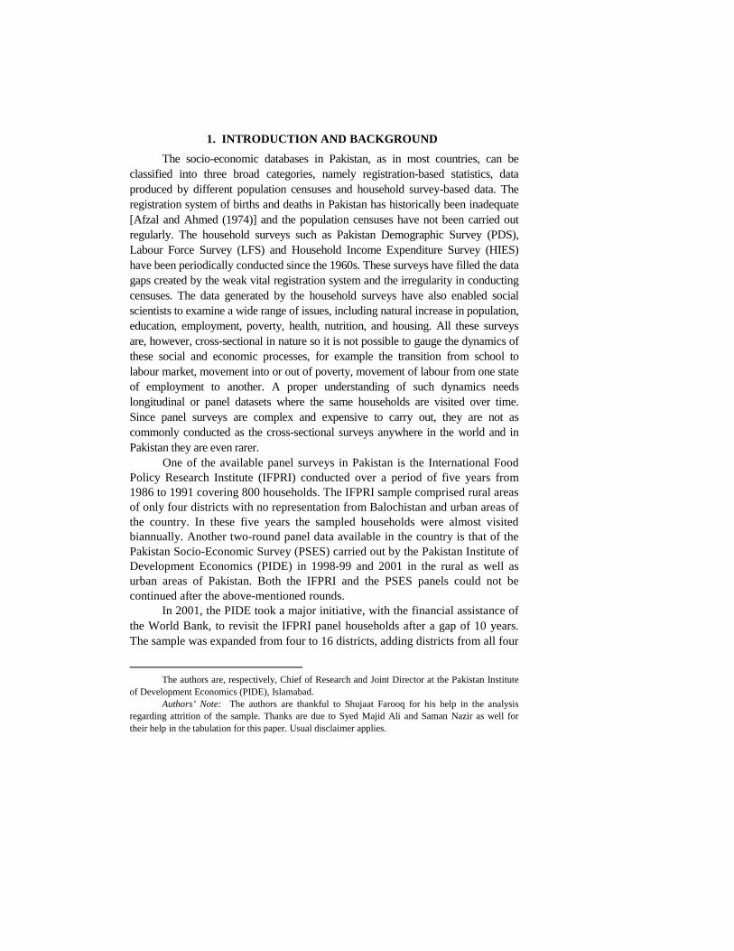
The scatter of the selected districts, as can be seen from Figure 1, is a good indicator of the geographical coverage of the districts covered under the PPHS. The sample covers the whole length of the country, strengthening its representativeness.

4

Fig. 1. Map Showing Selected Districts for the PPHS-2010

3. HANDLING THE SPLIT HOUSEHOLDS

Before discussing the sample size, it is important to understand how the split households have been dealt with in the panel survey. A split household is defined as a new household where at least one member of an original panel household has moved in and is living permanently. This movement of a member from a panel household to a new household could be due to his/her decision to live separately with his/her family or due to marriage of a female member. If not handled properly, the demographic composition of the sampled households is likely to change over time.

In the rounds two and three of the PRHS-PPHS split households were also interviewed. They, however, were only those households that were residing in the same village as the original panel household. In other words, movement of panel households or their members residing out of the sampled villages were not followed because of the high costs involved in this type of follow-up.

5

4. SAMPLE SIZE OVER THE DIFFERENT ROUNDS

The size of the sample for each round of the panel survey is shown in Table 2. The total size varies from 2721 households in 2001 to 4142 households in 2010. These variations, as discussed earlier, are for three reasons. First, the PRHS-II carried out in 2004 was limited to two provinces, Punjab and Sindh, while the other two rounds covered all four provinces. Second, in the PRHS-II as well as the PPHS-2010, split households were also interviewed (Table 2). Third, urban sample was added in the third round, PPHS, 2010.

As can be seen from Table 2, in the PRHS-I, carried out in 2001, the total sample consisted of 2721 rural households. The sample size decreased to 1614 households in PRHS-II (2004) because of the non-coverage of two provinces. However, 293 split households were interviewed in PRHS-II to raise the total sample size to 1907 households. Table 2 shows that in the PPHS-2010 the total rural households interviewed in four provinces were 2800, out of which 2198 were panel households and the remaining 602 were split households. With the addition of 1342 urban households, the total sample size of the PPHS 2010 accounted for a total of 4142 households (Table 2).

Table 2

Households Covered during the Three Waves of the Panel Survey

PRHS-I 2001

PRHS-II 2004 PPHS-2010 Panel house-holds

Split house-holds

Total Panel house-holds

Split house-holds

Total Rural house-holds

Urban house-holds

Total Sample

Pakistan 2721 1614 293 1907 2198 602 2800 1342 4142

Punjab 1071 933 146 1079 893 328 1221 657 1878

Sindh 808 681 147 828 663 189 852 359 1211

KP 447 – – – 377 58 435 166 601

Balochistan 395 – – – 265 27 292 160 452

Source: PRHS 2001, 2004 and PPHS 2010 micro-datasets.

Four features of the three rounds of the panel data are noteworthy, which

are as follows:

(i) Urban households, which have been included for the first time in the sample in the third round (PPHS) held in 2010, are not panel households as yet. Essentially, the urban sample can be analysed as a cross-sectional dataset at present and after their coverage in the next round of the survey they can be treated as panel households.

(ii) Split households are not strictly panel households, particularly those where a female has moved due to her marriage. Thus, the matching of

6

split households with the original panel households is not a straight- forward exercise. While doing any analysis the split households need to be handled carefully.

(iii) Only the rural sampled households in Punjab and Sindh are covered in all three rounds, so the analysis of the three-wave data is restricted to these two provinces.

(iv) For the analysis of all rural areas covering four provinces, panel data are available for the 2001 and 2010 rounds.

5. SCOPE OF THE PANEL SURVEY

The scope of the panel survey is examined in terms of the types of information (modules) gathered through the structured questionnaires. In all three rounds, two separate questionnaires for male and female respondents were prepared and different modules were included in these questionnaires (Table 3). A two-member team of enumerators, one male and one female, visited each sampled household to gather information. Female enumerators were responsible to fill the household roster and pass it immediately to her male counterpart. Education and employment modules were included in both male and female questionnaires but the relevant information regarding children (under 5 years old), both male and female, was recorded in the female questionnaire. One major objective of the PRHS-PPHS panel survey has been to examine the movement into or out of poverty therefore a detailed consumption expenditure module has been a part of the female questionnaire in all the three rounds. Expenditures on durable items, however, were recorded in the male questionnaire. Health and migration modules were included in PRHS-I and PPHS 2010 rounds. A module on household-run businesses and enterprises was part of the latter two rounds as well.

Each round of the survey has had certain specific areas of focus. Agriculture, for example, was the main focus of the PRHS-I when information even at the plot level was collected from the land operating households. In the other two rounds only a brief agriculture module was included. The main focus of the PRHS-II was mental health, dowry, inheritance and marriage-related transfers. The PPHS-2010 was conducted at a time when inflation was high and the nation had also faced some natural disasters including droughts and floods. In the latest round modules on shocks, food security, subjective wellbeing and overall security were specially included in the questionnaire.

In short, the scope of the three rounds of the panel survey is wide. A variety of social, demographic and economic issues can be explored from these rounds. While some core modules are common to all rounds, there are others that are specific to a certain round. Some of the information is, thus, cross-sectional in nature but can be linked to the household socio-demographic dynamics made available through the core modules.

7

Table 3

Scope of the Panel Survey: Modules included in Household Questionnaires

Modules PRHS-1 (2001) PRHS-II (2004) PPHS (2010) Male Female Male Female Male Female

Household Roster √ √ √ √ √ √ Education √ √ √ √ √ √ Agriculture √ × √ × √ × Non-Farm Enterprises √ × × × √ × Employment √ √ √ √ √ √ Migration √ × √ × √ × Consumption √ √ √ √ √ √ Credit √ × √ × √ × Livestock Ownership × √ × √ × √ Housing × √ × × × √ Health × √ × √ × √ Dowry and Inheritance × √ × √ × × Mental Health × × × √ × × Marital history and marriage related transfers × × × √ × × Shocks and Coping Strategies × × × × × √ Household Assets × × × × × √ Household food security × × × × × √ Security × × × × √ √ Subjective welfare × × × × √ √ Business and enterprises × × × × √ × Transfer/Assistance from programme and Individuals × × × × √ ×

6. AN ANALYSIS OF THE SAMPLE ATTRITION

As shown earlier, in the PRHS-PPHS data have been collected from the same households over three points of time- 2001, 2004 and 2010. It is common in such surveys that some participants (households) drop out from the original sample for a variety of reasons including geographical movement and refusal to continue being part of the panel. This attrition of the original sample represents a potential threat of bias if the attritors are systematically different from the non-attritors. It can lead to ‘attrition bias’ because the remaining sample becomes different from the original sample [Miller and Hollist (2007)]. If the participating units, however, are not dropped out systematically, meaning that there are no distinctive characteristics among the attriting units, then there is no attrition bias even though the sample has decreased between waves. It is, therefore, important to examine the attrition bias in our panel survey. 6.1. Theoretical Considerations1

Attrition in panel surveys is one type of non-response. At a conceptual level, many of the insights regarding the non-response in cross-sections carry

1This sub-section depends heavily on Arif and Biquees (2006) who have examined the

attrition bias between two rounds of the Pakistan Socio-Economic Survey (PSES) carried out in 1998-99 and 2001 by the Pakistan Institute of Development Economics.

8

over to panels. According to Fitzgerald, et al. (1998), attrition bias is associated with models of selection bias. Their statistical framework for the analysis of attrition bias, which has been used by several other studies [see for example, Alderman, et al. (20000; Thomas, et al. (2001); Aughinbaugh (2004)], makes distinction between selections on variables observed in the data and variables that are unobserved. Alderman, et al. (2000) believe that,

‘there is sample attrition, one determines whether or not there is selection on observables. For this purpose, selection on observables includes selection based on endogenous observables. For this purpose, selection on observables includes prior to attrition (e.g. in the first round of the survey). Even if there is selection on observables, this does not necessarily bias the estimates of interest. Thus, one needs to test for possible attrition bias in the estimates of interest as well’ [Alderman, et al. (2000)].

Assume that the object of interest is a conditional population density f(y|x) where y is scalar dependent variable and x is a scalar independent variable (for illustration, but in practice the extension to making x a vector is straightforward):

y= β0 + β1 + ε, y observed if A=0 … … … … (1)

where A is an attrition indicator equal to 1 if an observation is missing its value of y because of attrition, and equal to zero if an observation is not missing its value y. Since (1) can be estimated only if A=0 that is, one can only determine g(y|x, (A=0)), one needs additional information or restrictions to infer f(.) from g(.). These can come from the probability of attrition, PR(A=0|y, x, z), where z is an auxiliary variable (or vector) that is assumed to be observable for all units but not included in x. This implies estimates of the form:

A* = δ0 +δ1x + δ2z + V … … … … … (2)

A = I if A* ≥ 0 … … … … … … (3) = 0 if A* < 0

If there is selection on observables, the critical variables is z, a variable that affects attrition propensities and that is also related to the density of y conditional on x. In this sense, z is “endogenous to y”. Indeed, a lagged value of y can play the role of z if it is not in the structural relation being estimated is related to attrition. Two sufficient conditions for the absence of attrition bias due to attrition on observables are either (1) z does not affect A or (2) z is independent of y conditional on x. Specification test can be either of these two conditions. One test is simply to determine whether candidates for z (for example, lagged value of y) significantly affect A. Another test is based on Beketti, et al. (1988), and is known as BGLW test. It has been applied by Fitzgerald, et al. (1998) and Alderman, et al. (2000). In the BGLW test, the value of y at the initial wave of the survey (y0) is regressed on x and on A. This

9

test is closely related to the test based on regressing A and x and y0 (which is z in this case); in fact, two equations are simply inverses of one another [Fitzgerald, et al. (1998)]. Clearly, if there is no evidence of attrition bias from these specification tests, then one has the desired information on f(y|x). 6.2. Extent of Attrition

Table 4 presents the attrition rate for different rounds. Between 2001 and 2010, the attrition rate was around 20 per cent while the rate for the 2004 to 2010 period was 25 per cent, suggesting some households had dropped in 2004 and re-entered the panel in 2010. For the 2004-10 period, the highest attrition rate is found in Balochistan hinting towards more movement of sampled households than in other provinces.

Table 4

Sample Attrition Rates of Panel Households—Rural (%)

2001-2004 2001-2010 2004-2010 Pakistan 14.1 19.6 24.9 Punjab 12.9 17.1 23.8 Sindh 15.7 18.3 26.2 KPK – 16.1 – Balochistan – 33.2 –

Source: Authors’ computations based on PRHS 2001 and PPHS 2010 micro-datasets. 6.3. Attrition Bias

As stated earlier, the urban sample was included in the panel survey in 2010 for the first time and hence the attrition issue is related to the rural sample. It has also been noted that the PRHS-II was limited to two large provinces, Punjab and Sindh. All the rural areas were covered in round I (2001) and round III (2010). The attrition bias is examined between the two waves 2001 and 2010. Five models have been estimated where the dependent variable is whether attrition occurred between these two rounds (1= yes; 0 = no), results for which are presented in Table 5. The sample included in these models consists of all 2001 households and all regressors are measured in 2001.

Following Thomas, et al. (2001) and Arif and Bilquees (2006), the first model of attrition includes the only one covariate, In(PCE), where per capita consumption (PCE) is used as a measure of households’ economic status. Table 5 presents coefficient estimates from the logit regressions. The first model indicates that there is a statistically significant negative relationship between PCE and the probability of leaving the panel. On average, lower economic status households were more likely to attrite between the two waves, so without weighting the PPHS-2010 would be less representative of lower economic status households than would be a random household survey.

10

In model 2, two variables, ln(PCE) and ln(household size) have been included. Both increasing PCE and family size (in 2001) are significantly associated with a household staying part of the subsequent round of the panel survey. The third model in Table 5 adds one dummy, that of a household consisting of only one or two members. The association between attrition and PCE and household size still remains negatively significant. On the other hand, small size households (with 1 or 2 members) show a significant association with attrition.

Model 4 included measures related to three characteristics of the head of the household, which are age, sex and literacy. None of these variables turned out to be statistically significant. Two economic variables, ownership of livestock and land, and provincial dummies are added in model 5. Both the economic variables are significantly associated with keeping households part of the panel and maintaining them as non-attritors (see Table 5). Among the provinces, households in Balochistan are more likely to leave the sample than households located in other provinces. It is evident from the multivariate analyses that there is a positive association between leaving the panel and small household size. Improving economic status of the household is statistically significant to keep the household in the sample, so it is mainly the poorer households that are attriting.

Table 5

Determinants of Attrition through Logit Regression Correlates (2001/02) Model 1 Model 2 Model 3 Model 4 Model 5 Log per capita consumption –0.286* –0.342* –0.353* –0.214** –0.152*** Log household size –0.257* –0.177*** –0.014 0.056 Households with 1 or 2 family members only (yes=1) 0.416*** 0.426*** 0.353

Age of head of household (years) 0.001 0.003

Age-square of head of household 0.000 0.000

Female headed households (yes=1) 0.378 0.493***

Literacy of the head (literate=1) –0.138 0.010

Livestock owned (yes=1) –0.443* –0.451* land owned (yes=1) –0.280* –0.377*

Provinces (Punjab as ref.) Sindh –0.009 KPK –0.021 Balochistan 0.910* Constant 0.580 1.458** 1.36** 0.926 0.222 LR chi-square 11.93 (1) 19.35(2) 21.63(3) 53.71 (9) 102.63 (12) Log likelihood –1353.789 –1350.079 –1348.941 –1332.229 –1307.268 Observations 2,714 2,714 2,714 2,711 2,711

Source: Authors’ computations based on PRHS 2001 and PPHS 2010 micro-datasets. Note: ***P<0.01; ** P<0.05, * P<0.10.

11

As discussed in the beginning of this section, BGLW test, introduced and used initially by Becketti, et al. (1988), is the other method of testing the attrition bias. This test examines whether those who subsequently leave the sample are systematically different from those who stay in terms of their initial behaviourial relationships. We examine the consumption (lnPCE) equations as well as poverty equations but distinguishing two successively more restrictive subsets of participants—all 2001 households, and those still in the sample in 2010, labelled as ‘Always in’ or non-attritors.

Tables 6 and 7 present estimates of OLS regression for consumption equations and logit estimates for poverty equations respectively. A standard set of household and the head of the household characteristics, including age, and literacy of the head of the household, family size, and ownership of dwelling unit and livestock have been entered as independent variables into these equations. All the equations are significant, as can be seen from Table 6 and Table 7. These estimates indicate a number of associations that are consistent with widely-held perceptions about consumption behaviour and poverty. For example, age and literacy of the head of the households have a positive impact on consumption while they are negatively associated with poverty. A similar pattern of association was also found for family size as it has a positive association with poverty but a negative relation with the per capita consumption expenditure. The ownership of both livestock and land has a positive association with per capita expenditure, but a negative relation with the incidence of poverty.

Table 6

Household Expenditure: OLS Regression Model 2001-2010

Variables Full Sample ‘Always in’(Non-attrition) t-difference

test Coefficients St. Error Coefficients St. Error Age (years) –0.001 0.004 0.001 0.004 –0.500 Age2 0.000 0.000 0.000 0.000 0.000 Literacy (literate=1) 0.196* 0.023 0.190* 0.025 0.251 Family Size –0.032* 0.003 –0.036* 0.003 1.333 Land Ownership (yes=1) 0.255* 0.023 0.252* 0.025 0.125 Livestock 0.142* 0.025 0.133* 0.028 0.341 Own House (yes=1) –0.104** 0.047 –0.134** 0.055 0.592 Constant 6.838* 0.105 6.870* 0.117 –0.290 F-stat 56.46 47.66 – R-square 0.1305 0.1367 – Observations 2,642 2,115 –

Source: Authors’ computations based on PRHS 2001 and PPHS 2010 micro-datasets. ***P<0.01; ** P<0.05, * P<0.10.

Our interest here, however, is more in the difference that the attritors might have brought in the sample. To ascertain this we apply the t-difference test with the following hypotheses and assumption:

12

H0: No significant difference between attritor and non-attritor. H1: Significant difference exists between attritor and non-attritor. Assumption: unequal sample size, unequal variance.

The t-difference test results (see last columns of Table 6 and 7) show that there are no significant differences between the set of coefficients for the sub-sample of those lost to follow-up versus the sub-sample of those re-interviewed for indicators of either consumption or poverty. These estimates, therefore, suggest that the coefficient estimates of standard background variables are not affected by sample attrition.

Table 7

Correlates of Poverty: Logistic Regression Model 2001-2010

Correlates Full Sample ‘Always in’(Non-attritors) t-difference

test Coefficients St. Error Coefficients St. Error Age (years) 0.025 0.019 0.022 0.022 0.147 Age2 0.000*** 0.000 0.000 0.000 0.000 Literacy (literate=1) –0.545* 0.102 –0.504* 0.117 –0.376 Family Size 0.093* 0.011 0.108* 0.013 –1.257 Land Ownership (yes=1) –0.827* 0.102 –0.840* 0.116 0.120 Livestock (yes=1) –0.592* 0.105 –0.504* 0.122 –0.780 Own House (yes=1) 0.538** 0.210 0.639** 0.263 –0.430 Constant –1.817* 0.483 –1.994* 0.568 0.339 LR chi-square 206.39 160.22 – Log likelihood –1374.198 –1058.706 – Observations 2,642 2,115 –

Source: Authors’ computations based on PRHS 2001 and PPHS 2010 micro-datasets. *** P<0.01; **P<0.05; * P<0.1.

7. SOCIO-DEMOGRAPHIC PROFILE OF THE SAMPLE

One of the major advantages of a panel survey is to track the dynamics of any variable over time more precisely. A brief profile of the PRHS-PPHS sample is given here through selected socio-demographic characteristics, including mean household size, sex ratio, dependency ratio, age-sex structure, education and employment. Literature shows that these characteristics are linked to socio-economic well-being and are, therefore, good indicators to monitor the progress any population is making.

7.1. Mean Household Size and Sex Ratio

Many studies find household size being positively linked to poverty, and the PRHS-PPHS data conform to this trend, as can be seen from Table 8. Comparing the mean rural household size by consumption quintiles in PRHS-I, PRHS-II and the PPHS we find the sharpest decline in the richest quintile (Q5) where the household size reduced by 1.8 persons per household. On the contrary, the reduction in the household size for the poorer quintiles remain

13

much lower suggesting that the reduced overall size of the household is mainly due to the reduction in the household size of the top quintile (see Table 8). Also worth noting is the widening of the difference between the mean rural household size of the bottom (Q1) and top (Q5) quintiles from PRHS-1 in 2001 to PPHS-2010, increasing from a difference of 0.9 to 2.4 persons per household. Not surprisingly, the urban mean household size is smaller than the rural areas, as found in the PPHS-2010 (Table 8).

Table 8

Mean Household Size and Sex Ratio by Consumption Quintiles

Quintiles1

2001 2004 2010 Rural Only Rural Only Rural Urban Total

Mean Household Size All 8.3 7.8 7.8 7.1 7.6 Q1 9.2 9.2 8.9 8.5 8.8 Q2 8.5 8.2 8.3 7.4 8.0 Q3 8.2 7.9 7.9 6.9 7.6 Q4 7.9 7.5 7.3 6.7 7.1 Q5 8.3 6.3 6.5 6.2 6.9

Sex Ratio All 107.8 107.9 109.0 108.1 108.7 Q1 108.7 99.3 104.9 99.3 103.3 Q2 108.2 108.4 110.2 116.6 112.2 Q3 102.1 111.6 111.9 100.4 108.4 Q4 108.2 107.4 107.2 109.2 107.8 Q5 111.8 116.4 111.8 109.1 111.3

Source: Authors’ computations based on PRHS 2001 and PPHS 2010 micro-datasets. Note: 1-Quintiles based on per capita monthly consumption expenditure. Q1 is the quintile with least

per capita consumption expenditure.

Sex ratios found in the panel survey over the decade show no regular

pattern except that there is a constant male bias in it (Table 8). A trend that is visible for all rounds and regions, except in the one in 2001, is the lowest sex ratio for the bottom quintile (Q1). A possible reason for this trend can be out-migration of males from the poorest households depressing the sex ratio to a level lower than other quintiles (Table 8). 7.2. Dependency Ratio

The dependency ratio declines as we go up the quintiles for all the rounds of the PRHS and PPHS, as can be seen from Table 9. Comparing the rural dependency ratios in 2001, 2004 and 2010 we find a reducing trend over the years with the ratio declining from 86 to 71 over the decade. The decline from

14

2001 to 2010 is more pronounced for the lower quintiles (Q1, Q2 and Q3) where the dependency ratio reduced by a bigger margin than the top quintiles (Q4 and Q5).

There is much talk of the demographic transition taking place in the country resulting in declining dependency ratios, and Table 9 shows that this trend was found in the PRHS-PPHS sample as well. Further analysis will ascertain the exact nature and source of this decline but the reducing fertility is the primary cause of this decline as the proportion contributed by the child dependency in the total dependency has gone down over time.

Table 9

Dependency Ratio by Consumption Quintile

Quintiles 2001 2004 2010

Rural Only Rural Only Rural Urban Total

All 85.9 79.0 70.9 66.4 69.6

Q1 111.9 95.5 88.7 77.5 85.9

Q2 93.0 82.3 69.1 71.6 69.7

Q3 88.3 82.3 65.4 6.7 66.1

Q4 79.6 72.9 59.3 54.5 57.8

Q5 59.4 55.9 53.1 49.9 52.1

Source: Authors’ computations based on PRHS 2001 and PPHS 2010 micro-datasets. Note: 1-Quintiles based on per capita monthly consumption expenditure.

7.3. Age-sex Structure

Linked to the dependency ratio is the age-sex structure of a population. Figure 2 presents the age-sex structure of the three rounds of the PRHS-PPHS sample. The inference drawn in the previous section regarding decline in fertility is visible in the population pyramids B, C and D of Figure 2. Juxtaposing the three rural pyramids in Figure 2, that is A, B and D, we see a successively shrinking base with time implying a decline in fertility. It is interesting to note the movement of the bulge move up the rural pyramids over the three rounds of the PRHS-PPHS (Figure 2). For the PRHS-I it is the 0–4 years age group that is the heaviest, while for PRHS-II and PPHS they are the 5-9 years and 10-19 years, respectively.

The only urban pyramid (Figure 2 C) shows a more pronounced fertility decline than the rural areas. The base is much smaller and almost like an inverted pyramid till 19 years of age, suggesting that the initiation of the fertility decline took place in the urban areas of the panel sample earlier than the rural areas. A trend common to both rural and urban areas, however, is the male bias which is evident from all four pyramids of Figure 2.

15

Fig. 2. Age-sex Pyramids A: PRHS-1

2001 B: PRHS-II

2004

C: PPHS-2010 Urban

D: PPHS-2010

Rural

Male

Female Source: Authors’ computations based on PRHS 2001 and PPHS 2010 micro-datasets. Note: PRHS 1 and II were solely rural.

7.4. Head of Households—Their Sex and Age

The female-headed households are thought to be more prone to experience poverty but various studies in Pakistan have shown otherwise. The PRHS-PPHS sample also does not show any monotonic relationship between the female-headed households and economic situation of a household. The proportion of the female-headed households across the quintiles, as can be seen in Table 10, shows no singular trend. One trend, however, is evident from Table 2 and that is one of increasing size of the female-headed households. From 1.5 per cent of the rural households headed by females in 2001 the proportion increased to 4.3 per cent in 2010 (Table 10).

16

Table 10

Proportion of Female Headed Households and Mean Age1 of Household Heads by Sex

PRHS-I 2001

PRHS-II 2004

PPHS-2010

Rural Urban Total

Total Sample Female headed hhs3 (%) Mean age of male heads Mean age female heads

1.5 46.9 56.5

2.3 47.3 57.4

4.3 48.2 54.1

4.6 46.6 53.3

4.4 47.7 53.9

Quintile One2

Female-headed hhs (%) Mean age of male heads Mean age of female heads

1.5 45.9 57.3

1.9 47.5 56.0

4.5 46.7 49.5

7.7 46.1 47.2

5.3 46.6 48.7

Quintile Two Female-headed hhs (%) Mean age of male heads Mean age of female heads

1.5 47.5 60.1

0.9 47.1 62.3

4.1 48.0 52.4

2.7 45.6 61.3

3.6 47.2 54.6

Quintile Three Female-headed hhs (%) Mean age of male heads Mean age of female heads

2.4 46.4 47.5

2.5 47.7 56.5

4.3 48.4 56.4

4.8 47.2 54.5

4.5 48.0 55.7

Quintile Four Female-headed hhs (%) Mean age of male heads Mean age of female heads

2.4 45.9 49.2

3.4 50.5 55.4

3.5 48.9 56.7

4.1 46.2 54.2

3.7 48.0 55.8

Quintile Five Female-headed hhs (%) Mean age of male heads Mean age of female heads

2.6 48.8 56.0

4.4 50.4 50.8

5.4 48.9 53.2

4.7 47.3 55.1

5.2 48.4 53.8

Source: Authors’ computations based on PRHS 2001 and PPHS 2010 micro-datasets. Note: 1. Refers to mean age in years. 2. Quintiles refer to per capita monthly consumption

expenditure. 3. hhs refers to households.

Regarding the mean age of the head of the households it is interesting to

note that the female heads are averagely older than the male heads in a range of five to ten years over the period of the panel survey from 2001 to 2010 in the rural Pakistan (Table 10). Like the proportion of the female-headed households, no systematic trend is found for the difference between the mean ages of male and female head of households and consumption quintiles making it difficult to draw any inference regarding the sex of the head of the household and its economic well-being.

17

7.5. Marital Status

Apart from its social connotations, marriage in Pakistan becomes all the more important because fertility in the country mainly means marital fertility. Due to this factor the later the population marries the higher is the probability of fertility coming down. Figure 3 shows the proportion of the PRHS-PPHS sample never being married by sex and age. A clear pattern of increasing age at first marriage is evident, as the proportion never being married at the younger ages is seen increasing over time.

Fig. 3. Proportion Never-Married by Age and Sex (%)

Females

Males

PRHS-1

Rural PRHS-II

Rural PPHS

Rural PPHS

Urban

Source: Authors’ computations based on PRHS 2001 and PPHS 2010 micro-datasets.

18

If we focus on the 15–19 years age group in Figure 3 for the rural females, we see that an increase of 9 per cent takes place for the proportion never getting married from 2001 to 2010, rising from 74 per cent to 83 per cent (Figure 3). The increasing trend is maintained for the 20-24 year age group, as can be seen from the figure. Since males marry later than females, the maximum increase in the proportion never being married is exhibited ten years later than females, that is in the age group 25–29 years. From 2001 to 2010, 11 per cent more rural males were never married in the age group 25-29 years increasing from 36 per cent to 47 per cent. As expected, urban males and females remain never married till later in life than their rural counterparts (Figure 3).

7.6. Literacy Rates

Education is arguably the most representative social indicator. Despite its common usage definitional issues still confront it. In the PRHS-PPHS survey design as well as the questions probing the educational status have evolved over time. In the first round of the PRHS in 2001 educational status of the respondents were measured by the basic ‘ever been to school’ question. In the later round of the PRHS in 2004 and then PPHS in 2010 an additional question was asked probing the respondent if she/he ‘can read and write any language with comprehension’, as it was considered a better measure of literacy than just asking about attending school. This disparity in the basic measurement question regarding literacy makes it difficult to track its dynamics over the three rounds of the panel survey a little dodgy. The best solution in this scenario is to compare the literacy question of PRHS-II with only PPHS-2010 (shown in Table 11), and compare the ‘ever been to school’ trend across all the three rounds (presented in Table A5).

Total literacy levels of the PRHS-PPHS rural sample show an increasing trend in the six years from 2004 to 2010 with both male and female literacy increasing by over 12 per cent, as can be seen from Table 11. The gains are generally visible across all the ages below 40 years of age for both males and females. Literacy rates for the age groups from 40 years onwards need to be taken with caution as they show a slight downward trend for all the age groups for both males and females which is rather counter-intuitive (Table 11). A similar trend is found for the urban areas in the PPHS-2010 as well. This discrepancy can be simply due to faulty field operations or may have meanings that need to be explored more deeply.

Literature is replete with evidence related to positive association between economic well-being and education, and findings of the PRHS-PPHS conform to this trend as well. Literacy levels by consumption quintiles for PRHS-II and PPHS show a regular increasing trend as we go up the quintile ladder for both

19

Table 11

20

males and females (Table 11). Seen across the rounds, literacy rates for each quintile also show an increasing trend from 2004 to 2010 for both males and females. It is worth noting that the increasing literacy trend between the two rounds of the panel survey for each quintile is contributed more by increasing female literacy rates than males.

Coming to the ‘ever been to school’ question that was asked in all the three rounds of the panel survey, we see an increasing trend of going to school for both the sexes in 2004 from where it was in 2001 (Table A5 in the Annexure). The increasing trend seems to taper off in 2010 when we compare the rates with that for the round conducted in 2004. An over 10 percentage point gain in 2004 for females going to school in the younger age groups is a trend worth noticing. This spike in female rates can be a result of the various incentives that were being given by the government of the day to encourage girls’ education, an analysis of which is beyond the scope of this paper and would be dealt with separately. The discrepancy that we found in the literacy rates among the 40 plus age group (Table 11) is not found when we analyse the rates for those who have ever been to school. Needless to say, the rates for those who have ever been to school (Table A5) is higher than those who reported to be ‘literate’ (Table 11), and are higher for the urban areas than the rural areas for both the sexes.

7.7. Employment

Being a rural panel till the last round in 2010, the PRHS-1 and PRHS-II used rather complicated questions spread across various sections to primarily measure the agriculture employment rates among the survey households. With the addition of the urban sample to the panel design coupled with the motivation to simplify and improve the measurement of the labour force, it was decided to use the definition employed by the Labour Force Survey in Pakistan asking the question, ‘Did……. do any work for pay, profit or family gain during the last week, at least for one hour on any day?’, in the PPHS-2010.

Figure 4 presents the crude activity rate (CAR) and the refined activity rate (RAR) among the population aged 10 years and above in the PPHS-2010. The CAR expresses the percentage of the labour force in the total population while the RAR is the percentage of the labour force in the population of aged 10 years and above. Technically the RAR is a better measure for obvious reasons but the CAR has its value too. For countries like Pakistan that have the potential to benefit from the opportunity provided by the demographic transition, referred to as the demographic dividend, through the CAR we get to know the actual number of productive persons in the population.

21

Fig. 4. Crude and Refined Activity Rates (Age 10 Years and Above) by Sex and Region in PPHS-2010

(%)

Total Rural Urban

Source: Authors’ computations based on PPHS 2010 micro-dataset.

Looking at Figure 4 we see that the rural CARs and RARs are higher for

both males and females and understandably the RARs are higher than the CARs. The figure shows that less than half the population aged 10 years and above is active in the labour market (44 per cent) with the rate being lower for females (22 per cent) than males (64 per cent). Reaping the demographic dividend is about making use of the reduced dependency rate and the increasing size of the population in the working ages. A CAR of 34 per cent, pulled down mainly by the low female rate of 17 per cent, needs to be much higher for Pakistan to have any realistic chance of taking advantage of the demographic opportunity offered to it at present.

The low female participation rates that characterise Pakistan’s labour market are visible in the PPHS-2010 as well, as can be seen from Figure 5 where at no point more than one-third of the females are active in the labour market. Male activity rates conform to the traditional trend of an almost universal activity rate after 30 years of age till nearing 60 years of their lives, and hence appear as the usual inverted-U line in Figure 5. Female activity rates reach the highest towards the end of their reproductive age (45-49 years) before going down again as they grow old. At no stage in their lives, however, there is any drastic change in their activity rate and the variation remains confined to a limited range, as can be seen in Figure 5.

22

Fig. 5. Age Specific Activity Rates by Sex (%)

Total Male Female

Source: Authors’ computations based on PRHS 2001 and PPHS 2010 micro-datasets.

Unemployment can be the worst fear for anyone in the labour market.

The PPHS-2010 uses the same definition of unemployment as is used in the LFS in Pakistan, which is any person who is 10 years of age and above, and during the week preceding the survey is without work but is available for work and is seeking work. On the basis of this definition 11 per cent of the population is unemployed in Pakistan, as can be seen in Figure 6, with the rates being much higher for females (24 percent) than males (7 per cent). Looking the regional differences we find the unemployment rates to be higher in the urban areas (14 pe rcent) than the rural areas (10 per cent). This trend is followed by both males and females as the rate of their being unemployed is higher in the urban than in the rural areas. In fact, the unemployment rate is the highest for urban females (30 per cent), and if seen together with the low activity rates present a picture of reduced employment opportunities available to women- willing and seeking work but remaining unemployed.

Fig. 6. Unemployment Rate by Sex and Region (%)

Total Male Female

Source: Authors’ computations based on PRHS 2001 and PPHS 2010 micro-datasets.

23

8. CONCLUSIONS

The PRHS-PPHS panel is a rich source of information regarding a range of socio-economic and demographic processes, and a means to understand their dynamics over time. Along with having a few core modules the panel questionnaire is flexible enough to accommodate any particular area of interest in a specific round without affecting the overall efficiency of the survey design. Addition of the urban sample in 2010 to the previously all rural sample has made the panel design even more comprehensive. With three rounds having been carried out so far, in 2001, 2004 and 2010, the panel sample retains its qualities despite all the attritions and inclusions of split households.

The selected socio-demographic characteristics discussed in this paper indicate that most of the trends found in the PPHS sample conform to the existing body of literature. Even in cases where the trends deviate from convention we have the advantage to analyse them more deeply because of the longitudinal nature of the survey. The various rounds of the panel survey provide us both hindsight and foresight of sorts to understand the issues more clearly. Extensive modules on interrelated issues further help to analyse any covered area more thoroughly and holistically.

24

ANNEXURES

Table A1

Sample list for Pakistan Panel Household Survey 2010: Punjab Province Code District Code Tehsil Code Village Code

Punjab 1 Faisalabad 1 Faisalabad 1 Saddon 206RB 1 Jaranawala 2 Sing Pura 2 Gojra 3 Jarwanwala Chak 3 Summandri 4 Subdarawala 363JB 4

Khalishabad 356JB 5 Summandri 6

Attock 2 Feth Jang 5 Khirala Kalan 7 Pindi Ghaip 6 Thathi Gogra 8

Kareema 9 Hattar 10 Makyal 11 Gulyal 13 Dhock Qazi 14

Hafizabad 5 Pindi Bhatian 11 Khatteshah 53 Nasowal 54 Khidde 55 Bahoman 56 Daulu Kalan 57 Bagh Khona 58 Shah Behlol 59 Purniki 60 Thata Karam Dad 61 Mona 62

Vehari 6 Mailsi 12 Chak No 118–WB 63 Chak No 190 WB 64 Kot Soro 65 Chak No 195 WB 66 Mandan 67 Kot Muzzfar 68 Muradabad 69 Chak No 109 WB 70 Chak No 166- WB 71 Maqsooda 72

Punjab 1 Muzafar Garh 7 Ali Pur 13 Mail Manjeeth 73 Makhan Bela 74 Tibbah Barrah 75 Malik Arain 76 Kohar Faqiran 77 NauAbad 78 Kundi 79 Nabi Pur 81 Kotla Afghan 82

Bahawalpur 8 Ahmed Pur East 14 Ghunia 83

Chak No 157- N.P. 84

Haji Jhabali 85

Mad Rashid 87

Mukhawara 88

Pipli Rajan 89

Qadir Pur 90

Ladpan Wali 91

Chak Dawancha 92

25

Table A2

Sample list for Pakistan Panel Household Survey 2010: Sindh Province Code District Code Tehsil Code Village Code

Sindh 2 Badin 3 Badin 7 Kerandi 21

Golarchi 8 Kalhorki 22

Shaikhpur 23

Khoro 24

Khirdi 25

Bhameri 26

Walhar 27

Parharki 28

Golarchi 29

Lucky 30

Nurlut 31

Mitho Debo 32

Sorahdi 33

Chakri 34

Fatehpur 35

Mari Wasayo 36

Bajhshan 37

Khirion 39

Kandiari 40

Nawab Shah

9 Daulat Pur 15 Jagpal 93

Kandhari 94

Khar 95

Sindal Kamal 96

Kaka 97

Bogri 98

Manhro 99

Uttar Sawri 100

Mir Pur Khas

10 Kot G. Mohammad 16 Deh 277 101

Deh 320 102

Deh 346 103

Deh 339A 104

Deh 306 105

Deh 302 106

Deh 285 107

Deh 257 108

Larkana 11 Qamber Ali 17 Chacha 109

Rato Dero 18 Dera 112

Laktia 113

Do-Abo 114

Nather 115

Haslla 116

Sanjar Abro 117

Khan Wah 118

Khuda Bux 120

Naudero 121

Saidu Dero 122

26

Table A3

Sample list for Pakistan Panel Household Survey 2010: Khyber Pakhtunkhwa Province Code District Code Tehsil Code Village Code

KP 3 Dir 4 Blambut Adenzal 9 Katigram 41

Batam 42

Shah Alam Baba 43

Bakandi 44

Khanpur 45

Kamangara 46

Malakand 47

Khema 48

Khazana 49

Shehzadi 50

Munjal 51

Mardan 12 Takht Bhai 19 Khan Killi 125

Dagal 126

Jangirabad 127

Saidabad 129

Mian Killi 130

Fethabad 131

Seri Behial 133

L. Marwat 13 L. Marwat 20 Nar Akbar 135

Nar Langar 136

Alwal Khel 138

Gorka 141

Ghazi Khel 142

Table A4

Sample list for Pakistan Panel Household Survey 2010: Balochistan Province Code District Code Tehsil Code Village Code

Balochistan 4 Loralai 14 Loralai 21 Sanghri 145

Urd Shahboza 146

Sor Ghand 147

Nigang 148

Marah Khurd 149

Mekhtar 150

Tor 151

Khuzdar 15 Khuzdar 22 Bajori Kalan 153

Ghorawah 154

Bhat 155

Khat Kapper 156

Sabzal Khan 157

Khorri 159

Par Pakdari 160

Gawadar 16 Gawadar 23 Ankra 161

Chibab Rekhani 162

Dhorgati 163

Grandani 164

Nigar Sharif 165

Shinkani Dar 167

Sur Bandar 168

27

Table A5

28

REFERENCES

Afzal, M. and T. Ahmed (1974) Limitations of Vital Registration System in Pakistan against Sample Population Estimation Project: A Case Study of Rawalpindi. The Pakistan Development Review 13:3.

Alderman, H., J. Behrman, H. Kholer, J. Mauccio and S. Watkins (2000) Attrition in Longitudinal Household Survey Data: Some Tests for Three Developing Country Samples. The World Bank, Development Research Group Rural Development. (Policy Research Working Paper 2447).

Arif, G. M. and F. Bilquees (2006) An Analysis of Sample Attrition in PSES Panel Data. Pakistan Institute of Development Economics, Islamabad. (MIMAP Technical Papers Series No. 20).

Aughinbaugh, A. (2004) The Impact of Attrition on the Children of the NLSY97. The Journal of Human Resources 39:2.

Becketti, S., W. Gould, L. Lillard, and F. Welch (1988) The Panel Study of Income Dynamics after Fourteen Years: An Evaluation. Journal of Labour Economics 6.

Fitzgerald, J., P. Gottschalk, and R. Moffit (1998) An Analysis of Sample Attrition in Panel Data. The Journal of Human Resources 33:2.

Miller, R. and C. Hollist (2007) Attrition Bias. Department of Child, Youth and Family Studies, University of Nebraska-Lincoln.

Thomas, D., E. Frankenberg, and J. Smith (2001) Lost but not Forgotten: Attrition in the Indonesian Family Cycle Survey. The Journal of Human Resources 36:3, 556–592.