PACS photometry Data Analysis and Reprocessing...

PACS photometry Data Analysis and Reprocessing Tools Luca Calzoletti PACS Instrument and Calibration Scientist 27/10/2016

L. Calzoletti| Exploiting the Herschel Science Archive: Analysis/Processing Tools | ESAC | 27/10/2016 | Slide 2

Outline

1.  How to perform aperture photometry within HIPE 2.  How to reprocess data by means of interactive scripts


Useful and Interactive scripts

PACS Photometry Useful scripts are available in the Script menu within HIPE

PACS Photometry Interactive (IPipe) scripts are available in the Pipelines menu within HIPE •  IPipe are more handy, self-explaining scripts for reprocessing purposes (modify

parameters, save evaluation plots, …)


level 2 , 2.5 or 3 products

annularSkyAperturePhotometry

Point source photometry


Point source photometry


EEF_blu_20.txt EEF_grn_20.txt EEF_red_20.txt EEF_blu_60para_21.txt EEF_grn_60para_21.txt EEF_red_60para_21.txt EEF_blu_20para_21.txt EEF_grn_20para_21.txt EEF_red_20para_21.txt EEF_blu_60_22.txt EEF_grn_60_22.txt

Encircled Energy Fraction

•  EEF depends on the the observing mode (Prime/Parallel) and the scan speed (20”/s, 60”/s)

•  EEF tables are available at PACS Calibration Wiki page and in the next future as ADPs •  Only for standard modes (Prime, 20”/s), the HIPE task can be applied:

apphot = photApertureCorrectionPointSource(result,band='red',calTree=calTree)


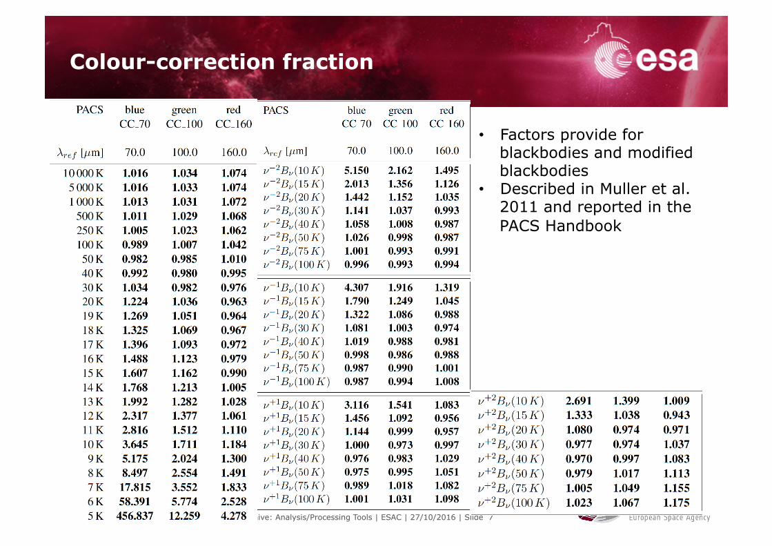
Colour-correction fraction

•  Factors provide for blackbodies and modified blackbodies

•  Described in Muller et al. 2011 and reported in the PACS Handbook


L3_pointSourceAperturePhotometry.py (single source)

•  It uses the annularSkyAperturePhotometry task •  Inputs: a list of fits files containing level 2 , 2.5 or 3 products

OBSLIST=['dra_red_25.fits’] •  Defaulf radii:

ap_blue = [12,35,45], ap_green = [12,35,45], ap_red = [22,35,45] •  Source positions are refined by means of the mapSourceFitter task •  Photometric error is provides as the rms of six background photometries (size =

annulus).

Point source photometry: useful scripts


OD OBSID AOR Target OBSMODE Filter Gain Dithering Repetitions PA (deg) ApertureRadius (") Peak Flux (Jy/pix) Pixel rms (Jy/pix) Flux (Jy) ApCorrFlux (Jy) Photometric error (Jy) xFWHM (") yFWHM (") 300 1342191958 gamDra_0004 gamma Dra Scan map red High false 1 99.4022187836 22 0.0125289214733 0.000120855918402 0.52377819326 0.640904703363 0.00504131240166 12.3112729904 10.4930814874

Point source photometry: useful scripts

L3_multipleSourceAperturePhotometry.py •  The input is an ASCII file:

Target1,12:34:56.7,-87:55:44.3 Target2,12h34m56.7s,-87d55m44.3s Target3,12.34567,-78.54321

•  Output text table:


JScanam Ipipe script

Few parameters to tune: •  deglitch = True: nSigmaDeglitch = 5 (default) •  galactic=True: just an offset is subtracted on baselineSubtraction Task •  stepAfter parameter into the scanamorphosMaskLongTermGlitches task

It projects frames after each pipeline step It shows evaluation plots


Unimap Ipipe script

The ipipe script invokes the Unimap MATLAB code by means the runUnimap task. The updated Unimap version, together with the free MATLAB runtime compiler, must be installed in the user computer. #Unimap installation directory path unimapDir = '/your/Unimap/directory’ #MATLAB MCR directory path mcrDir = '/your/MATLAB/Compiler/Runtime/directory' #The output files will be created and saved in the following directory:dataDir/#firstObsid_lastObsid_camera dataDir = '/your/data/directory’ Legacy maps available via HSA are generated with Unimap6.4.4. Compatibility of the Ipipe script is tested up to version 6.5.3, but results are not validated by the ICC Unimap memory optimized Ipipe script also is provided. It does not exploit the runUnimap task but, by subdividing the processing chain in two subsequent steps, it can save on RAM


Unimap parameters

•  Unimap depends on a large number of parameters. See the PDRG for details •  Unimap parameters are automatically optimized by default, according to the

characteristics (signal, extension,...) of each sky field. •  Files generated by runUnimap are left in the dataDir if cleanDataDir = True

•  Level1 frames formatted for Unimap: one FITS file per obsid and per band •  ASCII file with Unimap parameters (unimap_par.txt) •  Unimap LOG file (unimap_log.txt) •  Unimap output FITS maps: naïve, GLS, PGLS, WGLS •  Unimap evaluation FITS maps: Delta images

•  User can run several times the script by modifying the Unimap parameters and by saving the time for the generation of Level1 frames FITS files:

rewriteFramesFitsFiles = False

rewriteParametersFile = True: parameters are changed within the ipipe script False: unimap_par.txt is edited manually (just 9/40 parameters are pointed out in the ipipe script)


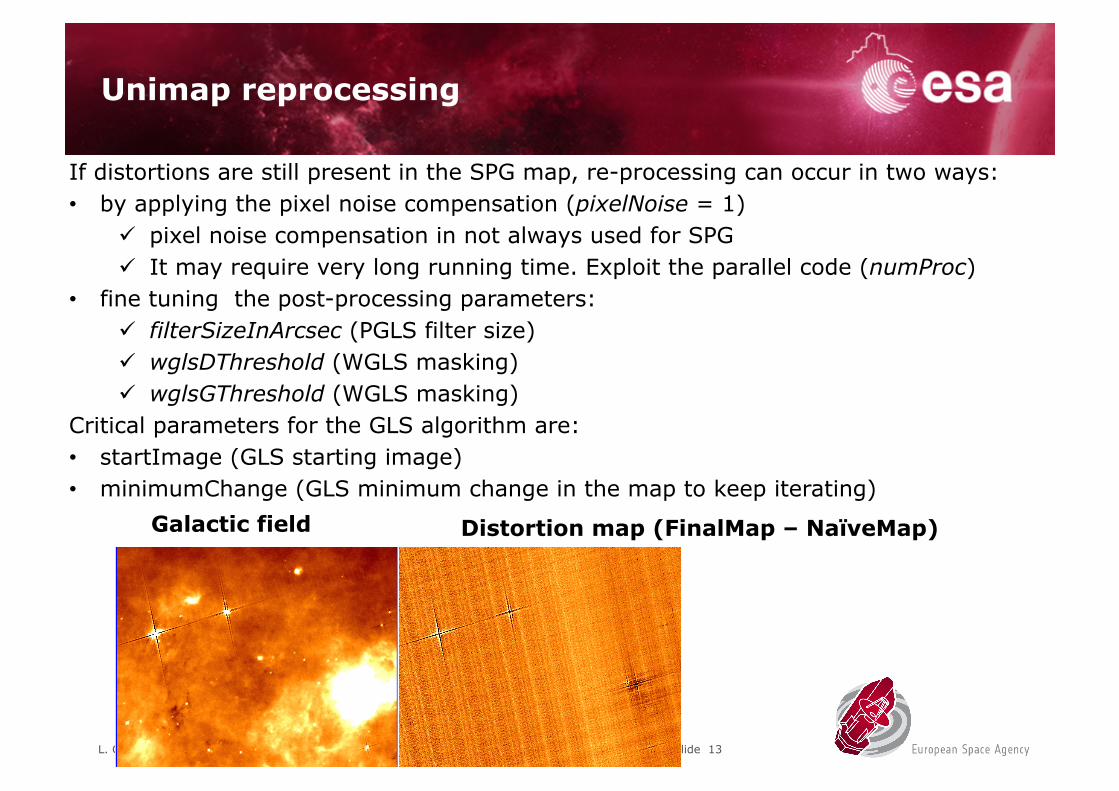
Unimap reprocessing

If distortions are still present in the SPG map, re-processing can occur in two ways: •  by applying the pixel noise compensation (pixelNoise = 1)

ü  pixel noise compensation in not always used for SPG ü  It may require very long running time. Exploit the parallel code (numProc)

•  fine tuning the post-processing parameters: ü  filterSizeInArcsec (PGLS filter size) ü  wglsDThreshold (WGLS masking) ü  wglsGThreshold (WGLS masking)

Critical parameters for the GLS algorithm are: •  startImage (GLS starting image) •  minimumChange (GLS minimum change in the map to keep iterating)

Galactic field Distortion map (FinalMap – NaïveMap)


QUESTIONS ?

PACS photometry Data Analysis and Reprocessing...

Documents

Transcript of PACS photometry Data Analysis and Reprocessing...