University of Tennessee, Knoxville University of Tennessee, Knoxville

TRACE: Tennessee Research and Creative TRACE: Tennessee Research and Creative

Exchange Exchange

Bulletins AgResearch

7-1991

Packing Fresh Vegetables in Tennessee: A Break-Even Analysis Packing Fresh Vegetables in Tennessee: A Break-Even Analysis

University of Tennessee Agricultural Experiment Station

Robert M. Ball

John R. Brooker

Robert P. Jenkins

Follow this and additional works at: https://trace.tennessee.edu/utk_agbulletin

Part of the Agriculture Commons

Recommended Citation Recommended Citation University of Tennessee Agricultural Experiment Station; Ball, Robert M.; Brooker, John R.; and Jenkins, Robert P., "Packing Fresh Vegetables in Tennessee: A Break-Even Analysis" (1991). Bulletins. https://trace.tennessee.edu/utk_agbulletin/448

The publications in this collection represent the historical publishing record of the UT Agricultural Experiment Station and do not necessarily reflect current scientific knowledge or recommendations. Current information about UT Ag Research can be found at the UT Ag Research website. This Bulletin is brought to you for free and open access by the AgResearch at TRACE: Tennessee Research and Creative Exchange. It has been accepted for inclusion in Bulletins by an authorized administrator of TRACE: Tennessee Research and Creative Exchange. For more information, please contact trace@utk.edu.

Bulletin 664July 1991

leking Fresh Vegetablesin Tennessee:

A Break-Even Analysis

Robert M. BallJohn R. BrookerRobert P. Jenkins

The University of TennesseeAgricultural Experiment Station

Knoxville, TennesseeD. O. Richardson, Dean

In Tennessee:

Packing Fresh Vegetables

A Break-Even Analysis

Robert M. BallJohn R. BrookerRobert P. Jenkins

University of TennesseeAgricultural Experiment Station

Knoxville, TennesseeBulletin 664, July 1991

AbstractA computer simulation program was used to estimate the break-even

volumes of five single-crop, one three-crop and two four-crop vegetablepackinghouse models. The packinghouse models were developed accord-ing to the economic-engineering approach. A representative study areawas selected to permit identification of appropriate vegetables. Out of anoriginal group of 15 vegetables, five were examined in two or more ofthe packinghouse models. Sensitivity analysis was also conducted on themulti-crop models to reveal the effects of adjustments in various specifi-cations regarding the operations of each model.

Packing three vegetables required 173 acres of tomatoes, 172 acres ofben peppers, and 344 acres of cabbage for the packinghouse to break even,with packing charges of $2.30, $3.00, and $2.55, respectively. Adding pota-toes as a fourth crop added another 136 acres to the amount required forthe packinghouse to reach the break-even point. Adding sweet corn in-stead of potatoes increased the total acreage by 375. Sweet corn requiredthe addition of an expensive hydrocooler, and potatoes required some spe-cial equipment, so total break-even volumes increased to cover higher fixedcosts. Average fixed, variable, and total cost curves were generated foreach vegetable.

IV

Table of ContentsABSTRACT iv

INTRODUCTION 1

OBJECTIVES 2

PROCEDURE 2

PACKINGHOUSE OPERATION 4

FACTORS AFFECTING OPERATING COSTS 6

PACKINGHOUSE INVESTMENT AND OPERATING COST 7Labor 7Packing Materials 8Administrative Expenses 8General Expenses 9Building, Equipment, and Land 9

PACKING CHARGES AND PRODUCT PRICES 9

RESULTS OF BREAK-EVEN SIMULATIONS 12Cabbage, Corn, Pepper, and Tomato Packinghouse 13Cabbage, Pepper, Potato, and Tomato Packinghouse 15Cabbage, Pepper, and Tomato Packinghouse 15Single-Crop Packinghouse Models 18Cost Curves For Three-Crop Packinghouse 25Effect of Selected Factors on Packing Costs 25

CLOSING REMARKS 31

REFERENCES 33

v

Packing Fresh VegetablesIn Tennessee:

A Break-Even Analysis

Robert M. Ball, John R. Brooker and Robert P. Jenkins * *

IntroductionThe recent decline in profitability for many traditionally Southern com-

modities and the increased profitability of other minor crops have forcedproducers to reexamine traditional farm production decisions [Estes andIngram). As a result, many farmers are considering vegetables for the com-mercial fresh market as a substitute or addition to their present sets ofproduction enterprises. Before undertaking commercial production, farm-ers should be aware of the unique production requirements and market-ing opportunities for vegetables. They should study the needs of thecommercial vegetable market and grow those crops that are most com-patible with their own resources [Runyan et al.).

In 1982, a total of 2,070 Tennessee farms with 30,096 acres were in-volved in the production of fresh vegetables [V. S. Bureau of Census). Asproducers switch from the more traditional commodities to productionof fresh vegetables, one problem to be solved is the establishment of con-sistent markets for their produce. The Tennessee fruit and vegetable in-dustry is characterized by numerous small-scale growers who producea large assortment of crops, even though there are several large scale

"Approved for publication in January, 1989.""Former Graduate Research Assistant and Professor, Dept. of Agri. Econ. and Rural So-ciology, Agri. Exp. Sta., and Professor, Dept. of Agri. Econ. and Resource Devel., Agri. Ext.Ser., Knoxville, Tennessee.

Tennessee growers [Brooker 1985). However, considering anyone par-ticular crop, Tennessee is a minor supply region with respect to total U.S.production.

The diversity of crops produced, widely scattered small-scale produc-tion, and relatively minor position with respect to total U.S. productioncreate serious market access barriers for Tennessee fruit and vegetablegrowers attempting to enter commercial wholesale markets. In order tointerest large-volume commercial buyers, new as well as experiencedsmall-scale vegetable producers have the option of organizing an assembly-packing facility to package and sell their produce collectively instead oftrying to perform these functions individually. The formation of a grow-ers"cooperative or growers' association provides an opportunity for pool-ing resources and for establishing a reputation of marketing qualityvegetables. Both aspects will help to open more marketing opportunitiesfor local production [Runyan et al.).

ObjectivesThere were three specific objectives of this study:1. to determine the costs involved in constructing and operating a pack-

inghouse facility for fresh vegetables,2. to analyze the impact on cost and returns from handling selected

combinations of fresh vegetables, and3. to analyze the sensitivity of returns from adjusting various specifi-

cations regarding the operation of each packinghouse model.

ProcedureApproaches to estimating packinghouse cost and efficiency relation-

ships may be grouped into three broad categories. One method is thedescriptive analysis of accounting data, which mainly involves combin-ing point estimates of average costs into various classes for comparativepurposes. A second method is the statistical analysis of accounting data,which attempts to estimate functional relationships by econometricmethods. The third method is to use the economic-engineering approach,which "synthesizes" production and cost relationships from engineeringdata or other estimates of the components of the production function[French). The economic-engineering approach was used in this study.

The total packinghouse production function is obtained by combiningthe production functions for the various operating stages or components.The "building blocks" for the stages of the production functions are thebuilding and equipment capacities and the associated input-output rela-tionships for labor, energy, and materials.

Once the production functions have been specified, the cost functionsare determined by applying factor prices. Short-run cost functions are ob-tained by the specification of a set of production techniques and their ca-

2

pacities (thus defining a unique hypothetical packinghouse) and computingvariable operating costs for a range of output rates up to or in excess ofthe design capacity limits.

To develop long-run cost functions, considerations must be given toall alternative stage production techniques and to the measurement ofprices of durable inputs. The usual procedure for the later is to specifyan expected life of the equipment, divide this into the installed cost, andadd an amount to cover the cost of borrowed capital, taxes, insurance,and in some cases, a portion of average maintenance costs.

The economic-engineering approach has been criticized for the lack offindings pertaining to diseconomies of scale. This has been attributed tothe use of constant input coefficients (especially for labor) and the inabil-ity to measure or account for coordination problems as plant scale in-creases. Furthermore, although the engineering approach may handletechnical aspects of production processes with considerable accuracy, es-timates pertaining to management, sales, and service activities are apt tobe very crude [French].

A computer simulation program was used to facilitate analysis of thesehypothetical packinghouse operations [Falk, Tilly, and Schatzer]. This com-puter program allows the user to adjust various components of the pack-inghouse model to observe the resulting effects on cost and returns. Inthis study the determination of the crop acreages necessary for the pack-inghouse model to break even was the primary focus of adjustments tothe base packinghouse model. In other words, after the crops were selectedand the acreages arbitrarily set at a beginning level, the computer pro-gram calculated the acreages required for this particular packinghousemodel to break-even financially. The computer simulation model adjuststhe initial acreages in unison. In an application to a particular situationthe model could be constrained to hold some crop acreages constant andforce the adjustments required to reach the break-even level on one ormore of the remaining crop acreages. If any of the input-output coeffi-cients of the packinghouse model are changed, such as the packing feecharged the grower or the cost of a particular piece of equipment, thenthe break-even acreage for each crop will change.

In order to facilitate specification of certain expenses, such as land andthe selection of crops to examine, a representative study area was chos-en. Grundy County and its seven contiguous counties were chosen as thestudy area. The small-scale production of vegetables in the study areanecessitated emphasis on the break-even acreages revealed the supply lev-els necessary to support a viable fresh vegetable packinghouse. Whetheror not the assumed Lo.b. price received for the packed products providesan adequate return to the grower is not examined in this report. Initially,15crops were examined in a multi-product packinghouse scenario. These15crops were identified as currently being grown, or suitable for growth,

3

in the study area. Based on analysis with the IS-crop model, the numberof crops included in two or more of the packinghouse models presentedin this report was reduced to five vegetables-bell peppers, cabbage, Irishpotatoes, sweet corn, and tomatoes. These five vegetables were selectedbecause of potential for development, current production in the area and/orexpressed interest in expanded production, and compatibility in a multi-product packinghouse.

Packinghouse OperationThe basic operations in a vegetable packinghouse are sorting, sizing,

grqding and packing. A floor plan of the model packinghouse is shownin Figure 1. Depending on the kind of produce, additional activities mayinclude degreening, curing, washing, bunching, chemical treatments, andprecooling [Akamine et al.l. The sequence of activities varies with differ-ent crops. These operations are essential preparatory steps to storage, trans-portation, and subsequent marketing.

High temperatures are detrimental to the keeping quality of fruits andvegetables. However, elevated produce temperature is inevitable, espe-cially when harvesting is done during hot days [Akamine et al.l. Precool-ing is a means of removing this field heat. The general aim is to slow downthe respiration of the produce, minimize the susceptibility to attack ofmicro-organisms, reduce water loss, and ease the load on the cooling sys-tem of the transport vehicle. Methods of precooling include air cooling,vacuum cooling, and hydro-cooling.

Most fruits and vegetables are washed after harvesting. Washing mayimprove the appearance of the produce if grime, soil, scale insects, sootymolds, etc. are present. Washing with a detergent will remove residuesof fungicides and insecticides.

Drying removes excess surface water from the vegetable. Heated airis blown on the vegetables as they pass through sponge roller conveyors.Drying may also be done by a series of rotating brush dryers made of softbristles. Minimum heat and dryer brush speed should be used to avoid'injury to the fruits. Some vegetables have a natural waxy layer on theouter surface that is partly removed by washing. A layer of wax appliedartificially with sufficient thickness and consistency to prevent anaero-bic conditions within the produce provides the necessary protection againstdecay organisms. Waxing is especially important if tiny injuries andscratches on the surface of the vegetable are present. These can be sealedby wax. Another advantage of waxing is the enhancement of the glossof certain vegetables. Appearance may be improved by waxing, thus mak-ing the produce more acceptable to consumers.

Truck Scales

Receiving Area

..o>.~>QoU

Pack

Pack

rade Weight Sizer

Meeting Workers' Workers' Refrigeration StorageRoom Restroom Restroom Units Areas

Bath

ReceptionManager's

OfficeArea Equipement OfficeOffice Storage

Figure 1. Layout for vegetable packinghouse model (not to scale).

Vegetables show considerable variations in quality due to genetic, en-vironmental, and agronomic factors. Grading is necessary to get suitablereturns commensurate with quality. Grades are based on soundness, firm-ness, cleanliness, size, weight, color, shape, maturity, and freedom fromforeign matter and diseases, insect damage, and mechanical injury.

After grading, the produce is sized for uniformity. Hand-sizing is use-ful for small-scale packing. One packer is assigned to each size. However,this method is inadequate for consistent separation of commodities intouniform size groups. For commercial operations various sizing devices arenecessary, based on either shape or weight of the produce. Sizing devicesmay consist of rollers that have varying spacing, conveyor lines with differ-ing size holes, or spring-balance scale cups.

Most vegetables require some refrigeration during storage and ship-ment. Mechanically refrigerated storage gives the packinghouse managersome flexibility to delay sales in anticipation of a more favorable priceat a later date.

Equipment capacities needed for storage facilities should be chosen sothat temperatures are lowered quickly as produce is loaded. Good insula-tion, sound design and construction, use of plastic curtains on doors, andloading in small batches can increase the refrigeration equipment's effi-ciency.

Factors Affecting Operating CostsPackinghouse size, season length, operating level, and total volume are

factors that affect the cost of fresh vegetable packinghouse operations.Evaluation of the feasibility (or profitability) of fresh vegetable packingoperations depends upon three necessary components: sufficient quanti-ties of the product at mutually acceptable prices, ability of the packing-house to operate efficiently, and ability of the organization to sell itsfinished product [Brooker and Pearson].

Workers usually insist on being paid for a minimum of four hours eachday they report for work. Therefore, a short supply of incoming fruit mayencourage the packinghouse manager to operate at less than desired ca-pacity in order to retain an adequate labor force.

A successful vegetable marketing organization must be able to assurecustomers that they will receive uniform quality produce. To fill require-ments of different classes of buyers, the packinghouse must use objec-tive grading standards and controls [Berberich]. Although quality issometimes only cosmetic, growers and packinghouse managers mustrecognize the importance of marketing and realize they must satisfy thebuyers standards and not their own [Motes et al.].

The quality of the incoming vegetables affects the operational efficien-cy of the packinghouse. If the quality is low, then the pack-out rate may

be limited by the number of graders. If quality is high, then dumpers andpackers may limit pack-out productivity. Because the percentage of cullsdepends on the quality of incoming produce, costs vary with changes inquality of incoming supplies.

Costs directly related to the number of hours a packinghouse operateswill also vary with quality. Quality influences costs through limiting thevolume packed in any given hour. With lower quality produce beingreceived by the packinghouse, either output will be lower or a longer num-ber of hours will be worked to pack the desired volume. In either event,those costs related to the hours of operation will increase. Therefore, costsdirectly related to the number of hours a packinghouse is operated areconsidered as quality associated costs [Bohall et al.l.

Quality will also affect costs which are fixed aggregate amounts peryear. With a given acreage of vegetables harvested and delivered to thepackinghouse, the total pack-out will decrease with poorer quality [Bo-hall et al.l. Hence, the fixed annual expenses must be spread over fewertotal crates of output, and average total cost per crate will rise.

Packinghouse Investment and Operating CostThe economic-engineering method was used to specify the investment

and operating cost of the vegetable packinghouses. Information was ob-tained for the cost of labor, packing materials, facilities, administration,land, general expenses, and cost of packing. The equipment was designedto pack-out 400 crates per hour when operating at 100 percent of ratedcapacity. This is the smallest size packing line that could be constructedwith the automatic sizing (weighing) machinery. Several operationalspecifications concerning the packing facility were necessary to facilitatethis analysis.

1. The packing facility has a beginning cash balance of $10,000. This may comefrom several varied sources such as producer fees, government support, or possi-ble funding from development oriented public agencies.

2. The organization is able to borrow ninety percent of the cost for equipment,facilities and operations to finance the operation at an interest rate of ten percent.The remaining ten percent of the cost for equipment, facilities and operations wouldhave to come from similar sources mentioned in assumption number one.

3. Payments on the building, machinery, and equipment are made quarterly.4. Salvage value is based on ten percent of initial value. The estimated life of

the grading and sizing equipment and hydrocooler is fifteen years. The conveyor,refrigeration, forklifts, scales, field crates and bulk bins have an estimated lifeof ten years and the building has an estimated life of twenty years.

5. The operating level of the packinghouse is set at 70 percent of rated capaci-ty, i.e., the pack-out rate is 280 crates per hour.

LaborThe number of workers required at each stage of the packing opera-

tion is presented in Table 1. It was presumed that only one product would

7

Table 1. Number of workers required at each station in a freshvegetable packinghouse designed to handle 400 crates perhour.

Bell Sweet Fall Spring IrishLabor Pepper Tomato Corn Cabbage Cabbage Potato

-----------------------------------------------workers -----------------------------------------------Dumper, Culls 2 2 2 2 2 2Forklift 1 1 1 1 1 1Dumper 2 2 2 2 2 2Unloading 0 0 2 2 2 0Grader 6 6 6 6 6 6Packer 20 20 20 20 20 20Crate Former 4 4 4 4 4 4Hydrocooler 0 0 2 0 0 0Storage 3 3 3 3 3 3Records 1 1 1 1 1 1

Source: Ball

be packed during a given work shift. While the packing line requires 20packers for the tomato line and 20 packers for the potato line, it mayormay not be the same 20 individuals. The packinghouse was designed tooperate as a multi-product facility, so the packing line was designed toutilize complementary equipment wherever possible.

The minimum wage of $3.35 per hour was paid to all the employeesexcept forklift operators. The forklift operator was paid a slight premiumabove minimum wage ($4.00 per hour) due to the special skills neededto operate the forklift. The State unemployment tax is 2.7 percent of thefirst $7,000. The Federal unemployment tax rate is 6.2 percent; but if theemployer pays the state tax on time, the law permits a 5.4 percent credit.

Packing MaterialsThe cost of 50-pound capacity potato bags was set at $0.44. Packaging

materials for bell peppers was set at $0.80 per 11/9 bushel waxed carton,20-pound cartons for tomatoes cost $0.95, 50-pound cartons for cabbagecost $1.10, and wire crates for 41/2 dozen ears of sweet corn cost $0.94.The cost of wooden pallets was covered by charging 19 cents per packedcrate.

Administrative ExpenseThe executive secretary was paid $5.00 per hour, for 40 hours per week

8

Building, Equipment and LandA blueprint design of the packing facility was obtained from Agri-Tech

Incorporated Uohnson]. The 25,000-square-foot building was estimatedto cost $500,000 (Table 2). The weight sizer costs $134,717, and was usedto size the tomatoes, bell peppers, and potatoes. The conveyor belt usedto grade and size the sweet corn and cabbage, cost $6,692. A hydrocooler,that was used only for sweet corn, cost $125,000. The field crates wereused by growers for delivering tomatoes and sweet corn to the packing-house. The bulk bins were used by the producers growing potatoes, bellpeppers, and cabbage.

The Monteagle, Tennessee area was chosen as a representative site lo-cation due to access to the interstate and because it is fairly centrally lo-cated within the study area. The Marion County tax office quoted thatland was selling for about $1,500 per acre and taxes would be $65 peryear. Three acres were needed for the hypothetical packinghouse.

[Snell]. The manager's salary was set at $24,000 per year. If a packingfacility hired an inspector for sixteen weeks (average length of a seasonl,it would cost the packinghouse about $8,000.

General ExpensesExpenses for utilities, telephones, office supplies, and postage are

presented in Table 2. The cost of office furniture, a computer system, type-writer, copy machine, check writer, and time clock were obtained fromappropriate business firms in Knoxville. An air conditioning/heater unitwas provided for the offices and reception area.

Packing Charges and Produce PricesCrop yields were based on the estimated yields published by the Ten-

nessee Agricultural Extension Service (Table 3). Market prices were speci-fied to be the average of those received on the Atlanta wholesale marketduring the summer months of 1982-1986 (Table 4). These Atlanta priceswere adjusted for brokerage fees and transportation expenses from thestudy area (Table 5). The computer model used in this study required theinput of selling prices received by the packinghouse. However, the possi-ble effect of fluctuations in the selling prices is neutralized in the modelbecause of the specification that growers receive the difference betweenthe selling price and the packing charge. Hence, the profitability of thepackinghouse is directly impacted by the volume packed and the per cratefee charged to the grower for packing the vegetables. The grower wouldbe impacted by volume packed and by the magnitude of the differencebetween selling price and packing fee.

9

Table 2. Initial investment and annual expenses for a fresh vege-table packinghouse.

Item Expense Amount

BUILDING AND EQUIPMENT:Building 125,000 square feet)Equipment (Weight Sizer)HydrocoolerRefrigeration UnitsForklift!-land ForkliftReturn Flow BeltField CratesBulk BinsTruck Scales

$500,000.00$134,717.00$125,000.00$ 20,000.00$ 18,500.00$ 2,000.00$ 6,692.00$ 45,000.00$ 40,000.00$ 30,000.00

1240' X 40', 5 Ton Units)lelectricl(manual, 4 at $500)Iconveyorl17500 @ $6.001(1000 @ $40.001

LAND:Current Value (3 acres @ $1,500/acrel $ 4,500.00

GENERAL:Office Furniture & Equipment

Furniture IReception area, Manager's Officeand Meeting Rooml

Computer SystemCopy MachineCheck WriterTime ClockAir Conditioning/Heating Units

$ 5,538.00$ 4,080.00$ 2,000.00$ 359.00$ 435.00$ 1,790.00

ANNUAL EXPENSESUtilitiesTelephoneOffice SuppliesProperty TaxesPostageInsurance on BuildingMaintenance & Repair on BuildingInsurance on Machinery & EquipmentMaintenance on Machinery & Equipment

$11,100.00$10,500.00$ 3,420.00$ 65.00$ 2,040.00$ 4,200.00$10,000.00

2%2%

Source: See Ball for details regarding sources of particular cost values.

10

Table 3. Crop yields specified for packinghouse feasibility analysis.

Crop Pounds per Crate Yield per Acre Marketablea

pounds crates percentIrish Potato 50 300 75Tomato 20 700 70Bell Pepper 40 350 75Sweet Corn 42 155 75Spring Cabbage 50 450 80Fall Cabbage 50 450 80

"Percentage of total yield that is marketable obtained from Jenkins and Rutledge.Source: Jenkins et al.

Table 4. Months vegetables packed, specified distribution of qual-ity, and product prices used in packinghouse models.

Quality" Selling Priceb

Crop Month #1 #2 #3 #1 #2 #3

-----------pecent ----------- --------------dollars --------------Irish Potatoes July 100 6.15Tomato July 40 40 20 7.47 7.47 3.72

August 40 40 20 7.15 7.15 3.75Sept. 40 40 20 6.38 6.38 3.19

Bell Pepper July 15 85 11.40 9.12August 15 85 9.01 7.21Sept. 15 85 11.17 8.94Oct. 15 85 9.51 7.61

Sweet Corn June 100 6.15July 100 5.89

Spring Cabbage June 100 7.34July 100 6.36

Fall Cabbage Oct. 100 4.95Nov. 100 4.93Dec. 100 5.90

"Distribution of packout by U.S.D.A. grade categories obtained from Rutledge, andJenkins.

hAverage monthly wholesale market price in Atlanta, 1982-1986, adjusted for transpor-tation and brokerage expenses from packinghouse study area [Neely].Source: Federal-State Market News Service.

11

Table 5. Freight and brokerage fees used to adjust Atlanta whole-sale market prices to Lo.b. packinghouse prices.

Crop Transportationa Brokerage Feeb

Irish PotatoTomatoBell PepperSweet CornSpring CabbageFall Cabbage

------------------------dollars per crate ------------------------0.30 0.100.30 0.250.24 0.250.18 0.250.30 0.150.30 0.15

"Transportation cost from Grundy County to Atlanta, Georgia.°Brokerage fee included in wholesale price quoted in Atlanta market.

Source: Neely.

The packing season in the study area for these four crops is June throughDecember (Table 6). The distribution of the crops among the seven monthsis an approximation and could be altered by weather conditions duringthe growing season and/or by adjustments in traditional planting dates.Coordination of the harvesting dates for each crop in order to assure aneven flow of incoming supplies over an extended harvesting season is crit-ical to the operation of the packinghouse.

Income to the packinghouse operation is generated by the packing feeit charges the growers. The packing fees specified in the base models wereobtained from two sources. The per crate packing charge for potatoes was$1.30, $2.30 for tomatoes, $3.00 for bell peppers, and $2.40 for sweet corn[Zwingli et al.]. The packing charge for cabbage was $2.55 per 50-poundbag [Kirkpatrick].

Results of Break-even SimulationsThe simulation results of three different packinghouse models are

presented in this section. First, a four-crop facility that packed tomatoes,bell peppers, sweet corn, and spring and fall cabbage. Second, a four-cropfacility without a hydro cooler that packed potatoes, tomatoes, bell pep-pers, and spring and fall cabbage. And third, a three-crop facility thatpacked tomatoes, bell peppers, and spring and fall cabbage. After examin-ing the impact of various factors on the crop acreages required for thepackinghouse to break even, each of the five crops was examined in asingle-crop packinghouse configuration. For each of these single-cropmodels, the assumed annual volume handled by the packinghouse wasvaried to measure cost scale relationships.

The acreage specified for each crop was set at an initial beginning pointand adjusted by the same percentage up or down, as guided by the com-

Table 6. Distribution of crops by harvest month, Grundy Countystudy area, Tennesseea.

MonthBell

PeppersIrish

Potatoes TomatoesSpring

CabbageFall

CabbageSweetCorn

............. -.- -.-.. ------ - -- percent .

June 50 25July 5 50 75 100 35August 45 35September 45 30October 5 45November 45December 10

"Study area includes Grundy and its seven contiguous counties.Source: Rutledge, and Jenkins.

puter program, until the volume handled by the packinghouse allowedit to operate at the break-even point. Except for sweet corn, all of the othercrop acreages were set equal to each other and vary a few acres in theresults because of rounding errors generated in the simulation model.Sweet corn acreage was arbitrarily set higher than the other crops becauseof the need to cover the cost of the expensive hydro-cooler.

Cabbage, Corn, Pepper, and Tomato PackinghouseThe facility packing cabbage, sweet corn, bell peppers, and tomatoes

requires a total of 1,064 acres (165 acres of tomatoes, 169 acres of bellpeppers, 400 acres of sweet corn, 165 acres of spring cabbage and 165acres of fall cabbage) to operate at the break-even level (Table 71.Whilethe total number of crates delivered to the packinghouse was 385,150crates, 290,513 crates were packed. This is because of the specificationthat 30 percent of the tomatoes, 25 percent of the bell peppers, 25 per-cent of the sweet corn, and 20 percent of the cabbage would not bemarketable.

Even though this four-crop packinghouse model breaks even financiallyunder the specified conditions, the cost of packing sweet corn and springand fall cabbage exceeds the specified packing charge. However, the costof packing tomatoes and bell peppers is less than the packing charge. Thepackinghouse model uses the profitable difference in the packing costsand packing charges for tomatoes and bell peppers to offset the negativedifference in the packing cost and packing charge for the sweet corn andspring and fall cabbage. To prevent the packing charge for one vegetablefrom being used to subsidize the cost of packing another, the packing-house manager would probably need to readjust the packing charges. Ex-cept for sweet corn, the acreages of the other crops were purposely kept

13

Table 7. Facility packing four crops: crop acreage, volume packed, cost per crate, and packing charge at thebreak-even level of operations.

Acres Yield Total Volume Average Cost PackingCrop Harvested Per Acre Received Packed Variable Fixed Total Charge

Number ----------------------------Crates ---------------------------- -----------------------------------Dollars -----------------------------------Tomato 165 700 115,500 80,850" 1.70 0.54 2.23 2.30Bell Pepper 169 350 59,150 44,363b 1.53 0.94 2.48 3.00Spring Cabbage 165 450 74,250 59,400c 1.85 0.78 2.63 2.55Fall Cabbage 165 450 74,250 59,400c 1.85 0.78 2.63 2.55Sweet Corn 400 155 62,000 46,500d 1.73 1.27 3.00 2.40

Total 1064 385,150 290,513

"Assuming 70-percent of harvested tomatoes are marketable.bAssuming 75-percent of harvested bell peppers are marketable.cAssuming 80-percent of harvested cabbages are marketable.dAssuming 75-percent of harvested sweet corn is marketable.

close to being equal to each other since the goal was to reveal minimumacreages for a packinghouse to break even. An unconstrained optimizingmodel would of course eliminate the total acreage of any crop that receiveda packing charge lower than the cost of packing. Another constraint placedon the packing-house simulations is the higher acreages specified for sweetcorn. This was permitted because of the high cost of the hydrocooler,which is necessary for the proper handling of sweet corn.

Cabbage, Pepper, Potato, and Tomato PackinghouseThe second packinghouse model was designed to pack four crops, but

in contrast to the first model, sweet corn was replaced by Irish potatoes.This eliminated the expense of a hydrocooler. At the break-even level ofoperation, this packinghouse model requires 150 acres of potatoes, 167acres of tomatoes, 168 acres of bell peppers, 170 acres of spring cabbage,and 170 acres of fall cabbage (Table 81.The total crop acreage is reducedfrom 1064 in the first model to 825 in this second model. The mainadjustment is the replacement of the 400 acres sweet corn by 150 acresof potatoes. The required acreages of tomatoes, bell peppers, and cabbageremained near the same levels.

The average cost of packing potatoes and spring and fall cabbage ex-ceeds the per crate packing charge. The cost of packing tomatoes and bellpeppers is less than the per crate packing charge. As with the first pack-inghouse model, the simulation program uses the difference in the pack-ing cost and packing charge of tomatoes and bell peppers to offset thedifference of the packing cost and packing charge of the potatoes and cab-bage. The model is constrained to pack at least 150 acres of potatoes. Other-wise, based on the $2.23 per crate cost of packing and the $1.30 per cratepacking charge, the logical actions would be to eliminate potatoes or in-crease the packing charge.

Cabbage, Pepper, and Tomato PackinghouseBased on the results of the two four-crop packinghouse models, this

third model is designed to pack three crops-tomatoes, bell peppers, andcabbage. With the packing charges at the same values as those used inthe two four-crop models, the break-even crop acreages results in a pack-out of 253,760 crates (Table 9). This is a smaller number of crates for thepackinghouse to handle than either of the four-crop break-even models.As expected with this smaller volume, the average fixed cost at the break-even point increases and average variable cost remains constant, thus forc-ing average total cost to increase. The cost of packing tomatoes increasesfrom $2.24 in the four-crop model to $2.33 per crate in this three-cropmodel, which is slightly higher than the specified packing charge of $2.30.Bell peppers remain on the positive side, and cabbage becomes even morecostly per crate in comparison to the packing charge.

15

Table 8. Facility packing four crops without a hydrocooler: crop acreage, volume packed, cost per crate, andpacking charge at the break-even level of operations.

Acres Yield Total Volume Average Cost PackingCrop Harvested Per Acre Received Packed Variable Fixed Total Charge

Number .......................... Crates .......................... ................................. Dollars .................................

Tomato 167 700 116,900 81,830" 1.70 0.54 2.24 2.30Bell Pepper 168 350 58,800 44,100b 1.53 0.85 2.38 3.00Spring Cabbage 170 450 76,500 61,200c 1.85 0.78 2.63 2.55Fall Cabbage 170 450 76,500 61,200c 1.85 0.78 2.63 2.55Irish Potato 150 300 45,000 33,750d 1.17 1.06 2.23 1.30

Total 825 373,700 282,080

"Assuming 70·percent of harvested tomatoes are marketable.bAssuming 75·percent of harvested bell peppers are marketable.cAssuming 80·percent of harvested cabbages are marketable.dAssuming 75·percent of harvested sweet corn is marketable.

Table 9. Facility packing four crops: crop acreage, volume packed, cost per crate, and packing charge at thebreak-even level of operations.

Acres Yield Total Volume Average Cost PackingCrop Harvested Per Acre Received Packed Variable Fixed Total Charge

Number ----------------------------Crates ---------------------------- -----------------------------------Dollars -----------------------------------Tomato 173 700 121,100 84770" 1.70 0.64 2.33 2.30Bell Pepper 172 350 60,200 45: 150b 1.53 1.04 2.57 3.00Spring Cabbage 172 450 77,400 61,920c 1.85 0.90 2.75 2.55Fall Cabbage 172 450 77,400 61,920c 1.85 0.90 2.75 2.55

Total 689 336,100 253,760

"Assuming 70-percent of harvested tomatoes are marketable.bAssuming 75-percent of harvested bell peppers are marketable.

•...• cAssuming 80-percent of harvested cabbages are marketable.--.:)

Single-Crop Packinghouse ModelsAnalysis of the three multi-crop models indicates that not all vegeta-

bles are able to cover their packing cost with the specified packing charge.To determine the economies of scale associated with packing each vegeta-ble included in the multi-crop models, each vegetable was examinedseparately in single-crop packinghouse models. The only adjustment inthe fixed cost items was the addition or deletion of any specialized equip-ment needed by a particular vegetable. The assumed volumes handledby the packinghouse are varied to generate the appropriate cost functions.

The average cost curves for a single-crop facility packing potatoes isillustrated in Figure 2. When the packing charge is set at $1.30, whichis the fee specified in the multi-crop models, the packinghouse is requiredto pack 1,575,000 crates of Irish potatoes to reach the break-even levelof operation. At the previously specified levels of yield and quality, itwould require 7,000 acres to obtain this volume. Irish potatoes would beharvested during July in the study area. If the packinghouse operated 24hours a day for 31 days at 100 percent of rated capacity (400 crates perhour), the facility could pack-out 297,600 crates. If the packing chargeis raised to $2.07, the facility could break-even with a pack-out of 225,000crates. However, to handle this volume in 31 days would require a pack-out of 7,259 crates per day. To handle this volume at 400 crates per hour,the facility would still need to operate 18 hours per day. It is unrealisticto assume that a packinghouse could operate at 100 percent of rated ca-pacity for 18 to 24 hours per day over an extended period of time. Therewould be problems with obtaining the required labor force, break-downof equipment, and difficulty securing a continual flow of incoming sup-plies to keep the packing facility operating smoothly.

The shape of the average total cost curve emphasizes the importanceof attaining the economies of scale available from increasing the volumehandled. This is especially true at the smaller volume levels when thecost curve declines rapidly with increases in output. While the examina-tion of a single-crop packinghouse cost curve can be discouraging, becauseof the large volume required to break even, it does provide considerableinsight into the need to have adequate packing fees and product volumesto support a economically viable packinghouse. It also supports the con-cept of packing complementary products to increase the total volumepacked over the entire season.

A single-crop facility packing tomatoes must handle approximately343,000 crates to reach the break-even level of operation (Figure 3). Thispack-out volume would require 700 acres of tomatoes. Because tomatoesare harvested during July, August, and September in the study area, thepackinghouse has a longer operating season than the single-crop potato model. Therefore, the total volume could be handled in 12

18

3.02.82.62.42.2

Q).•... 2.00'-U 1.8'-Q) 1.6n.(/) 1.4'-

>-' 0<.0

01.2

Cl 1.00.80.60.40.2

00

Average total cost

/Packingcharge ~1.30

Break-even point(1.575.000 crates)

\~ Average variable cost

2

Figure 2. Relationship between cost per crate and volume of potatoes packed in a single-crop packing house.

Average fixed cost

0.2 0.8 1 1.2 1.4Millions of Crates

1.81.60.4 0.6

weeks if the facility operated at 100 percent of rated capacity (400 cratesper hourI, for 72 hour per week. At the previously specified level of oper-ating over a packing season at 70 percent of rated capacity (280 cratesper hourI, the packinghouse would need to run 102 hours per week forthe full 12 weeks. Raising the packing charge from $2.30 to $2.75 reducesthe required break-even volume to 200,000 crates.

The single crop model for bell peppers is presented in Figure 4. It shouldbe noted that bell peppers are the only vegetable that had a packing chargethat exceeded the derived packing cost in all three multi-crop packing-house models examined in the previous section. The packing charge forbell peppers was specified as $3.00 per crate. Hence, the packinghousewould need to pack-out 140,000 crates to operate at the break-even point.This would require about 533 acres of bell peppers. The harvest seasonfor bell peppers is July, August, September, and October. To handle thisvolume in 16 weeks at an operating level of 280 crates per hour wouldrequire a pack-out of 8,750 crates per week, which would take slightlyless than 32 hours per week. If the packing facility were to decrease thepacking charge to $2.81, the total pack-out needed to maintain the break-even level of operation would be 157,800 crates (about 600 acresl. Pack-ing this larger volume would require the facility to operate 36 hours perweek for 16 weeks.

In the single-crop facility packing sweet corn, with a packing chargeof $2.40, the packinghouse would need to pack-out 290,000 crates to breakeven (Figure 5). Producers would be required to harvest 2,495 acres ofsweet corn to supply the required volume. Sweet corn is harvested in Juneand July (8 weeks), so the facility would need to pack-out 36,250 cratesper week. Operating at the 70-percent of rated capacity level, the facilitywould be required to operate 131 hours per week. To accomplish this task,the facility would be required to operate 19 hours per day, 7 days perweek. The packinghouse would encounter the same problem as the sin-gle crop facility packing Irish potatoes, since maintaining a labor forceand operating the facility for this length of time 7 days per week wouldcreate several problems. If the packing charge for sweet corn is raisedto $2.89, the break-even volume would be reduced to 117,000 crates. Tohandle this volume in eight weeks, the packinghouse hours of operationwould be reduced to 53 hours per week.

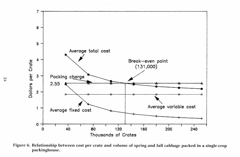
In the multi-crop models, the packing charge for spring and fall cab-bage is not high enough to cover the cost of packing. With the packingcharge value of $2.55, a single-crop facility packing cabbage would needto pack about 131,000 crates to reach the break-even point (Figure 61.Ap-proximately 364 acres at the specified yield could provide this volume.

20

7~-------------------------------,6 Average total cost

5 /C).•..0L-()

•• Break-even pointL-CD

(343.000 crates)a.lI)

3Packing /N L-

Charge,•.... 0(50 2.30

2

~ \ Average1 Variable

Average fixed cost Cost

00 200 -400

Thousands of Crates

Figure 3. Relationship between cost per crate and volume of tomatoes packed in a single-crop packinghouse.

10

9

8

7Q)

-+oJ0 SL.

UL.

5Q)0.

N UlN

L. 40

00 3

2

Average total

/cost

Break-even point(140,000 crates)

Packing charge /3.00 ~&---=--ir--~-&-----ir-------'=~--=::::t:==~

Average fixed cost-----~

Average Variable cost ---'"

o SO 80 100 120

Thousands of Crates1S0 20018020 40 140

Figure 4. Relationship between cost per crate and volume of peppers packed in a single-crop packinghouse.

7"'T"'"--------------------------------,6

Average total cost

5 /Q)+JCL-() 4L-Q) Break-even point0-

m 3 / (290.000 crates)L-N CW

00

2

Average variable cost

Average fixed cost ~

00 200 400

Thousands of Crates

Figure 5. Relationship between cost per crate and volume of sweet corn packed in a single-crop packinghouse.

7 ....•....-----------------------------------,

6

5

Average total cost

Cl) 4 / Break-even point+'0 (131.000)L..()

/L..3

N Cl)+>- a.

mL..

0(5 2Cl ,

I Average variable costAverage fixed cost

00 40 80 120 160 200 240

Thousands of Crates

Figure 6. Relationship between cost per crate and volume of spring and fall cabbage packed in a single-croppackinghouse.

Spring cabbage is harvested in June and July and fall cabbage is harvestedin October, November, and part of December. This would provide a pack-ing season of about 18 weeks in total. The packing facility would needto pack an average of 7,278 crates per week. Operating at 70-percent ofrated capacity (280 crates per hour), the facility could handle this weeklyvolume in 26 hours per week.

Cost Curves for Three-Crop PackinghouseAnalysis of the single crop packinghouse models reveals that several

crops require a larger volume than the facility could handle during a typicalharvesting period. To examine the impact of a multi-crop packinghousemodel on the packing cost curves, the three-crop model presented earlierwas used to generate the data. The cost curves should be observed as aset, in that the break-even acreages of tomatoes, bell peppers, spring cab-bage, and fall cabbage were determined simultaneously. From this break-even beginning point, the acreages of all three crops were increased anddecreased in unison. The resulting increase and decrease in volume packedallowed the cost curves to be estimated (Figures 7, 8, and 9).

Operating at the break-even level of operation would require 88,000crates of tomatoes, 32,000 crates of bell peppers, and 160,000 crates ofspring and fall cabbage. At these levels, the packing charge is equal tothe packing cost for each individual vegetable.

If the packinghouse manager was able to contract producers to plant800 acres (equally distributed among tomatoes, peppers, spring cabbage,and fall cabbage), the packinghouse would be able to pack-out 98,000crates of tomatoes (packing charge set at $2.30); 52,600 crates of bell pep-pers (packing charge set at $3.00); and 144,000 crates of spring and fallcabbage (packing charge set at $2.55). The packing charge exceeds pack-ing cost for tomatoes and bell peppers, but packing cost exceeds packingcharge by $0.05 for spring and fall cabbage. If the acreage planted wasincreased to 1000 acres and distributed equally among the crops, the pack-inghouse would be capable of packing out 122,500 crates of tomatoes,65,750 crates of bell peppers, and 180,000 crates of spring and fall cab-bage. By leaving the packing charges at $2.30 for tomatoes, $3.00 for bellpeppers, and $2.55 for spring and fall cabbage, each vegetable packingcharge would cover the packing cost.

Effect of Selected Factors on Packing CostsSensitivity of the cost functions from the three multi-crop packinghouse

models is discussed in this section. The interest rate, level of financing,operating level, and packing charge were varied from the values used togenerate the base solutions of the four-crop with a hydrocooler, four-cropwithout a hydrocooler, and the three-crop packinghouse models. The ef-fect on investment and operating costs, and on pack-out volume requiredto maintain the break-even level of operation, are presented in Table 10.

25

7-r---------------------------------,

C) 5-aL-UL- 4 Break-even pointC)a. / (32.000 crates)enL-a 3N

0'\ 0Pa~ingccharge23.00

1 Average ~ Average fixed costvariablecost

00 20 40 60 80 100 120

Thousands of Crates

6

Figure 8. Relationship between cost per crate and volume of peppers packed in a three-crop packinghouse.

7..,......----------------------------,

Average total cost

L.Q)Q.

(I) 3L.

ooo 2

/ Break-even point(88,000 crates)

~ Average variable cost

Average fixed cost

o 80 100. 120·.tAG

Thousands of Crates

Figure 7. Relationship between cost per crate and volume of tomatoes packed in a three-crop packinghouse.

.! 5oL-U

N00

L-Q)0-

ft)L-o(5o

7 ...•...------------------------------,

6

cost

Break-even point(160,000 crates)

Figure 9. Relationship between cost per crate and volume of cabbage packed in a three-crop packinghouse.

3Packing /charge~2.55 ~\.....--........--..;;;;poT===t:==::=::===::==:

2 " .Average vanable cost~

Average fixed cost

04-- -.....--..,.....-......--T"""""-.----,---+---..---r---r---,....-...,.....-""T"""---fo 80 120 160

Thousands of Crates

Table 10. Sensitivity of packinghouse cost and pack-out to adjustments in the interest rate, proportion ofinvestment financed, operating level, and packing charge.

Operating PackingPackinghouse model Interest Rate Financing Level Chargetotal costs, andpack-out 8% 12% 80% 50% 90% + $0.10

----------------------------------------------Percentage change from base solution ----------------------------------------------Four-crop:"

Fixed Cost -7 +7 -4 0 0 0Variable Cost -8 +7 -5 +62 -21 -18Crates Packed -8 +7 -5 +43 -15 -18

N Four-crop: (With hydrocooler)'<.D Fixed Cost -7 +7 -4 0 0 0

Variable Cost -7 +8 -4 +58 -20 -17Crates Packed -7 +8 -4 +40 -13 -17

Three-crop:dFixed Cost -7 +7 -4 0 0 0Variable Cost -7 +7 -4 +55 -19 -17Crates Packed -7 +7 -4 +37 -13 -17

"Packing charges were increased $0.10above the packing cost derived in the base solution."Cabbage, peppers, potatoes, and tomatoes.'"Cabbage, corn, peppers, and tomatoes.dCabbage, peppers, and tomatoes.

The interest rate was decreased from the solution level of 10 percentto 8 percent and also increased to 12 percent to reveal the impact of thisfactor on the break-even position of the packinghouse models. As antici-pated, the direction of the cost change coincided with the decrease or in-crease in the specified interest rate. For all three multi-crop packinghouses,the two percent change in the interest rate resulted in a seven to eightpercent change in total costs. This decrease (increase) in cost allowed thesimulation model to decrease (increase) the pack-out volume required forthe packinghouse to break even.

In the base solutions, a specification was included regarding the per-centage of the total investment being financed with borrowed capital. Thispercentage was reduced from 90 percent to 80 percent to observe the im-pact on the break-even analysis. Reducing the required level of financing10 percent generated a four percent reduction in both cost and pack-outof the break-even simulations of the three multi-crop packinghouses.

The percentage of rated pack-out capacity at which a packinghouseoperates is referred to as the operating level. This factor identifies the ef-ficiency of the packinghouse with respect to utilization of rated capacity.Few processing operations -run at 100 percent of rated capacity over anentire processing season. In most processing plants the percentage wouldvary during the season. The level selected for the base solutions was 70percent. Total fixed cost is not affected by adjustments in the operatinglevel. However, reducing the operating level to 50 percent had a substan-tial impact on variable cost. In the four-crop model without the hydro-cooler the total variable cost increased 62 percent (Table 10). This variablecost increase was associated with a 43 percent increase in the pack-outvolume required for the packinghouse to break even at this lower levelof operating efficiency. The impact on the other two packinghouse modelswas similar, but not quite as severe. This fact emphasizes the importanceof being able to operate the packinghouse at a high percentage of ratedcapacity. Operating at a low level of rated capacity increases the per cratevariable cost, thereby forcing the simulation model to require largervolumes to reduce average fixed cost until it eventually compensates forthe higher variable cost.

Increasing the level of operating efficiency to 90 percent reduced thetotal variable cost of the packinghouse approximately 20 percent in allthree models (Table 10). The cost reduction was possible due to the smallerpack-out necessary to reach the break-even level of operation. An impor-tant point here is the level at which the packinghouse operates has sub-stantially more impact on the economic viability of the packinghouse thanmoderate adjustments in the interest rate or financing level.

As noted earlier, the per crate packing charges entered into the threebase packinghouse models were obtained from sources reporting actual

30

industry rates. The simulation results also revealed the inadequacy of someof the packing fees when compared to the per crate packing cost of themodel packinghouse operating under the specified conditions. Using theper crate packing cost calculated in the break-even analysis of the threemodels as base values, the packing charges were adjusted to be $0.10 abovethe base value for each vegetable. This modification resulted in an increasein the packing charge for cabbage, corn, and tomatoes and a decrease forpeppers. The adjustment in packing fees did not affect total fixed cost(Table 10). With each crop supposedly paying its own way, the pack-outvolume required for the packinghouse to operate at the break-even pointdropped about 17 percent.

CLOSING REMARKSAmong the three multi-crop packinghouse models presented, the re-

quired pack-out volume for the operations to reach the break-even pointwas lowest when only three vegetables were being handled. The addi-tion of potatoes to a product group of tomatoes, bell peppers, and cab-bage did absorb some of the fixed cost, but changes in the break-evenacreages of the original three commodities were nominal. This was primar-ily due to the specified packing changes. Similarly, the addition of sweetcorn instead of potatoes to the packinghouse product mix substantiallyincreased the fixed expense because of the need for a hydrocooler. Tobreak even the packinghouse needed to pack the sweet corn from 400acres, plus nearly the same acreages of tomatoes, peppers, and cabbageas required by the three-crop model.

The impact on operating costs from adjustments in the specified pack-ing charges for each crop was visually emphasized in the cost curves gener-ated for the single-crop packinghouse models. Without any other productsto help cover part of the fixed expenses the break-even volumes identi-fied for each product were substantially higher than in the multi-cropmodels. The L-shaped acreage total cost curves for each vegetable revealedthe economics of scale available to the packing operation that can increasethe volume packed. The single-product cost curves also emphasized thenecessity for growers and packinghouse managers to agree on a packingcharge that is reasonable-a fee that allows the packing operation to beeconomically viable and also allow the grower to receive an adequatereturn for supplying the products. Growers receipts from the packinghousewill vary in response to industry wide supply and demand conditions be-cause of the normal price variation in vegetable prices within a market-ing season and from season to season. The packinghouse's receipts willdepend directly upon the volume handled, and sometimes the volume han-dled will be larger when Lo.b. prices are low. This possible conflict be-tween the interests of the growers and a packinghouse may be resolvedby the development of a packing fee based partially on the Lo.b. price.

31

While the single-crop packinghouse cost curves provide insight into thepacking fees that may be appropriate at various pack-out levels, the multi-crop packinghouse cost curves reveal the need to examine particularscenarios. The three-crop and two four-crop models presented in thisreport were selected to illustrate the volumes required for the packing-house model to break even. The packing charges were set at current in-dustry levels. Growers working together in a packing cooperative, ordealing with an independent packinghouse, should consider the packingfee appropriate for that particular packinghouse.

Analysis of the sensitivity of packinghouse costs and returns revealedthe substantial impact of the specified operating level. Adjusting the oper-ating level from 50 to 70 to 90 percent of rated capacity dramatically il-lustrated the importance of operating a packing facility as close to fullcapacity as possible. Adjustments in the specified interest rate and per-centage of investment being financed also affected the packinghouse, butless dramatically.

The packinghouse scenarios examined in this report provide introduc-tory evidence for application in a unique feasibility study. In other words,growers and packers need to work together to determine the selectionof crops to be packed and the acreage committed to the packinghouse.Then they should assess the likelihood of both the growers and the pack-inghouse attaining satisfactory net returns.

32

ReferencesAkamine, E. K., H. Kitagawa, H. Surbamanyam and P. G. Long. "Pack-

inghouse Operations." Postharvest Physiology Handling, and Utilizationof Tropical and Subtropical Fruits and Vegetables. Edited by E. R. B. Pan-tastico, the AVI Publishing Company, Inc., Westport, Connecticut,1975.

Ball, Robert Mason. "An Economic Feasibility Study For A Fresh Vege-table Packing Facility," M.S. Thesis, Dept. of Ag. Econ. and Rur. Soc.,Univ. of Tenn., Knoxville, Aug. 1988.

Berberich, Richard S. Small Fresh Fruit and Vegetable Cooperative Opera-tions. USDA Farmer Cooperative Service, FCS Information 106, June,1977.

Bohall, Robert W., Joseph C. Podany and Raymond O. P. Farrish. Pack-ing Mature Green Tomatoes: Quality, Costs, and Margins in the lower RioGrande Valley of Texas. USDA Economic Research Service MarketingResearch Report No. 635, November, 1963.

Brooker, John R., and James L. Pearson. Factors Affecting the EconomicFeasibility of Single Product Packinghouse Operations: Cantaloupes, Car-rots, Onions, and Radishes. Department of Agricultural EconomicsFlorida Agricultural Experiment Stations, University of Florida, Gaines-ville, Agricultural Economics Report 36, April, 1972.

Brooker, John R. An Assessment of the Structure of Fruit and Vegetable Mar-keting in Tennessee. Department of Agricultural Economics and RuralSociology, University of Tennessee Agricultural Experiment Station,Knoxville, Tennessee, Research Report 85-04, April, 1985.

Estes, Edmund, and Dewayne L. Ingram. "A Survey Perspective on Al-ternative Farming Programs in the South." Alternative Farming Oppor-tunities for the South. Proceedings of a Regional Conference, MississippiState University, January, 1987.

Falk, Constance, Daniel S. Tilley and R. Joe Schatzer. The Packing Simula-tion Model User's Manual. Department of Agricultural Economics, Ok-lahoma State University, Stillwater, Oklahoma, 1986.

Federal-State Market News Service. Atlanta Fresh Fruit and VegetableWholesale Market Prices, issue for 1982-1986, A.M.S., U.S.D.A.:Washington, D.C.

33

French, Ben C. "The Analysis of Productive Efficiency in Agricultural Mar-keting: Models, Methods, and Progress." A Survey of Agricultural Eco-nomics Literature, Vol. 1, Minneapolis, University of Minnesota Press,1977.

Jenkins, Robert P. Marketing Tennessee Fruits and Vegetables. TennesseeAgricultural Extension Service, University of Tennessee, Knoxville, Ten-nessee, Publication 1151, May, 1985.

Jenkins, Robert P., Larry Johnson, Alvin D. Rutledge, David L. Lockwoodand Robert M. Ray. Planning Budgets for Fruits and Vegetables. EC 890,Agricultural Extension Service, The University of Tennessee, January,1988.

Johnson, Larry. Sales Representative for Agri-Tech Incorporated, Wood-stock, Virginia. Telephone conversation concerning cost of packingequipment, September 24, 1987. Written correspondence concerningequipment cost and design, October 15, 1987.

Kirkpatrick, Tammy. Department of Agricultural Economics Virginia Poly-technic Institute and State University, Blacksburg, Virginia. Telephoneconversation and written correspondence concerning packing chargesof various packing facilities, January 4, 1988.

Motes, James E., Daniel S. Tilley and Raymond Joe Schatzer. "Vegetablesas Alternative Crops." Alternative Farming Opportunities for the South.Proceedings of a Regional Conference, Mississippi State University,January, 1987.

Neely, Leroy. Neely Wholesale Produce Company, Knoxville,Tennessee.Telephone conversation and visit to Neely Produce concerning cost offreight and brokerage fees, July 22, 1987.

Runyan, Jack L., Joseph P. Anthony, Jr., Kevin M. Kessecker and HaroldS. Ricker. Determining Commercial Marketing and Production Opportu-nities for Small Farm Vegetable Growers. USDA Agricultural MarketingService Marketing Research Report 1146, July, 1986.

Rutledge, Alvin. Tennessee Agricultural Extension Service Plant and SoilSpecialist, University of Tennessee, Knoxville, Tennessee, June 16,1987.

34

Zwingli, M. E., J. L. Andrian, W. E. Hardy and W. J. Free. Wholesale Mar-ket Potential for Fresh Vegetables Grown in North Alabama. AlabamaAgricultural Experiment Station, Auburn University, Bulletin 586, July,1987.

Snell, Larry. General Manager of Cumberland Farm Products, Monticello,and Russell Springs, Kentucky. Information obtained during personalinterview, October 30, 1987.

U.S. Bureau of Census, Census of Agriculture, 1982, Vol. I, Geographic AreaSeries, Part 42, Tennessee: State and County Data, U.S. Departmentof Commerce, May, 1984.

35

THE UNIVERSITY OF TENNESSEEAGRICULTURAL EXPERIMENT STATION

KNOXVILLE, TENNESSEE 37996-4500Ell-041S-QO-OO2-92

Agricultural Committee, Board of TrusteesJoseph E. Johnson, President of the University;

Amon Carter Evans, Chairman;L. H. Ivy, Commissioner of Agriculture, Vice Chairman;

Houston Gordon, R. B. Hailey, William Johnson, Jack Dalton;D. M. Gossett, Vice President for Agriculture

STATION omCERSAdministration

Joseph E. Johnson, PresidentD. M. Gossett, Vice President for Agriculture

D. O. Richardson, DeanT. H. Klindt, Associate DeanJ. I. Sewell, Associate Dean

William L. Sanders, Statistician

Department HeadsH. Williamson, Jr., Agricultural Economics and Rural Sociology

D. H. Luttrell, Agricultural EngineeringK. R. Robbins, Animal Science

Bonnie P. Riechert, CommunicationsCarroll J. Southards, Entomology and Plant Pathology

Hugh O. Jaynes, Food Technology and ScienceGeorge T. Weaver, Forestry, Wildlife, and Fisheries

Michael Zemel, NutritionG. D. Crater, Ornamental Horticulture and Landscape Design

John E. Foss, Plant and Soil ScienceJacquelyn Dejonge, Acting. Textiles, Merchandising. and Design

BRANCH STATIONSAmes Plantation, Grand Junction, James M. Anderson, SuperintendentDairy Experiment Station, Lewisburg. H. H. Dowlen, SuperintendentForestry Experiment Station: Locations at Oak Ridge, Tullahoma,

and Wartburg. Richard M. Evans, SuperintendentHighland Rim Experiment Station, Springfield, D. O. Onks, SuperintendentKnoxville Experiment Station, Knoxville, John Hodges III, Superintendent

Martin Experiment Station, Martin, H. A. Henderson, SuperintendentMiddle Tennessee Experiment Station, Spring Hill, J. W. High Jr., Superintendent

Milan Experiment Station, Milan, John F. Bradley, SuperintendentPlateau Experiment Station, Crossville, R. D. Freeland, Superintendent

Tobacco Experiment Station, Greeneville, Philip P. Hunter, SuperintendentWest Tennessee Experiment Station, Jackson, James F. Brown, Superintendent