Package ‘ursa’

Package ‘ursa’May 23, 2021

Type Package

Title Non-Interactive Spatial Tools for Raster Processing andVisualization

Version 3.9.4

Author Nikita Platonov [aut, cre] (<https://orcid.org/0000-0001-7196-7882>)

Maintainer Nikita Platonov <[email protected]>

Description S3 classes and methods for manipulation with georeferenced raster data: read-ing/writing, processing, multi-panel visualization.

License GPL (>= 2)

URL https://github.com/nplatonov/ursa

BugReports https://github.com/nplatonov/ursa/issues

Depends R (>= 3.0.0)

Imports utils, graphics, grDevices, stats, rgdal, png, jpeg

Suggests proj4, sf (>= 0.6-1), raster, ncdf4, locfit, knitr,rmarkdown, tcltk, sp, methods, fasterize, IRdisplay, caTools,shiny, rgeos, tools, webp, htmlwidgets, htmltools, leaflet,leafem, leafpop, RColorBrewer, ragg, widgetframe, geojsonsf (>=2.0.0), leaflet.providers

NeedsCompilation yes

ByteCompile no

Repository CRAN

Date/Publication 2021-05-22 23:50:02 UTC

R topics documented:ursa-package . . . . . . . . . . . . . . . . . . . . . . . . . . . . . . . . . . . . . . . . 4allocate . . . . . . . . . . . . . . . . . . . . . . . . . . . . . . . . . . . . . . . . . . . 4as.array . . . . . . . . . . . . . . . . . . . . . . . . . . . . . . . . . . . . . . . . . . . 5as.data.frame . . . . . . . . . . . . . . . . . . . . . . . . . . . . . . . . . . . . . . . . 7as.integer . . . . . . . . . . . . . . . . . . . . . . . . . . . . . . . . . . . . . . . . . . 9

1

https://github.com/nplatonov/ursa

https://github.com/nplatonov/ursa/issues

2 R topics documented:

as.matrix . . . . . . . . . . . . . . . . . . . . . . . . . . . . . . . . . . . . . . . . . . . 10as.Raster . . . . . . . . . . . . . . . . . . . . . . . . . . . . . . . . . . . . . . . . . . . 11as.raster . . . . . . . . . . . . . . . . . . . . . . . . . . . . . . . . . . . . . . . . . . . 14as.table . . . . . . . . . . . . . . . . . . . . . . . . . . . . . . . . . . . . . . . . . . . 15as.ursa . . . . . . . . . . . . . . . . . . . . . . . . . . . . . . . . . . . . . . . . . . . . 16bandname . . . . . . . . . . . . . . . . . . . . . . . . . . . . . . . . . . . . . . . . . . 18band_group . . . . . . . . . . . . . . . . . . . . . . . . . . . . . . . . . . . . . . . . . 20band_stat . . . . . . . . . . . . . . . . . . . . . . . . . . . . . . . . . . . . . . . . . . 21blank . . . . . . . . . . . . . . . . . . . . . . . . . . . . . . . . . . . . . . . . . . . . 22c . . . . . . . . . . . . . . . . . . . . . . . . . . . . . . . . . . . . . . . . . . . . . . . 24chunk . . . . . . . . . . . . . . . . . . . . . . . . . . . . . . . . . . . . . . . . . . . . 25close . . . . . . . . . . . . . . . . . . . . . . . . . . . . . . . . . . . . . . . . . . . . . 26codec . . . . . . . . . . . . . . . . . . . . . . . . . . . . . . . . . . . . . . . . . . . . 27colorize . . . . . . . . . . . . . . . . . . . . . . . . . . . . . . . . . . . . . . . . . . . 28colortable . . . . . . . . . . . . . . . . . . . . . . . . . . . . . . . . . . . . . . . . . . 32commonGeneric . . . . . . . . . . . . . . . . . . . . . . . . . . . . . . . . . . . . . . . 34compose_close . . . . . . . . . . . . . . . . . . . . . . . . . . . . . . . . . . . . . . . 35compose_design . . . . . . . . . . . . . . . . . . . . . . . . . . . . . . . . . . . . . . . 37compose_legend . . . . . . . . . . . . . . . . . . . . . . . . . . . . . . . . . . . . . . 41compose_open . . . . . . . . . . . . . . . . . . . . . . . . . . . . . . . . . . . . . . . 43compose_panel . . . . . . . . . . . . . . . . . . . . . . . . . . . . . . . . . . . . . . . 47compose_plot . . . . . . . . . . . . . . . . . . . . . . . . . . . . . . . . . . . . . . . . 48create_envi . . . . . . . . . . . . . . . . . . . . . . . . . . . . . . . . . . . . . . . . . 49cubehelix . . . . . . . . . . . . . . . . . . . . . . . . . . . . . . . . . . . . . . . . . . 52dim . . . . . . . . . . . . . . . . . . . . . . . . . . . . . . . . . . . . . . . . . . . . . 54discolor . . . . . . . . . . . . . . . . . . . . . . . . . . . . . . . . . . . . . . . . . . . 55display . . . . . . . . . . . . . . . . . . . . . . . . . . . . . . . . . . . . . . . . . . . . 56display_brick . . . . . . . . . . . . . . . . . . . . . . . . . . . . . . . . . . . . . . . . 58display_rgb . . . . . . . . . . . . . . . . . . . . . . . . . . . . . . . . . . . . . . . . . 59display_stack . . . . . . . . . . . . . . . . . . . . . . . . . . . . . . . . . . . . . . . . 60envi_files . . . . . . . . . . . . . . . . . . . . . . . . . . . . . . . . . . . . . . . . . . 62Extract . . . . . . . . . . . . . . . . . . . . . . . . . . . . . . . . . . . . . . . . . . . . 63focal_extrem . . . . . . . . . . . . . . . . . . . . . . . . . . . . . . . . . . . . . . . . 65focal_mean . . . . . . . . . . . . . . . . . . . . . . . . . . . . . . . . . . . . . . . . . 67focal_median . . . . . . . . . . . . . . . . . . . . . . . . . . . . . . . . . . . . . . . . 68focal_special . . . . . . . . . . . . . . . . . . . . . . . . . . . . . . . . . . . . . . . . 70get_earthdata . . . . . . . . . . . . . . . . . . . . . . . . . . . . . . . . . . . . . . . . 72glance . . . . . . . . . . . . . . . . . . . . . . . . . . . . . . . . . . . . . . . . . . . . 74global operator . . . . . . . . . . . . . . . . . . . . . . . . . . . . . . . . . . . . . . . 78groupGeneric . . . . . . . . . . . . . . . . . . . . . . . . . . . . . . . . . . . . . . . . 80head . . . . . . . . . . . . . . . . . . . . . . . . . . . . . . . . . . . . . . . . . . . . . 82hist . . . . . . . . . . . . . . . . . . . . . . . . . . . . . . . . . . . . . . . . . . . . . . 83identify . . . . . . . . . . . . . . . . . . . . . . . . . . . . . . . . . . . . . . . . . . . 84ignorevalue . . . . . . . . . . . . . . . . . . . . . . . . . . . . . . . . . . . . . . . . . 86is.na . . . . . . . . . . . . . . . . . . . . . . . . . . . . . . . . . . . . . . . . . . . . . 88legend_align . . . . . . . . . . . . . . . . . . . . . . . . . . . . . . . . . . . . . . . . . 89legend_colorbar . . . . . . . . . . . . . . . . . . . . . . . . . . . . . . . . . . . . . . . 90legend_mtext . . . . . . . . . . . . . . . . . . . . . . . . . . . . . . . . . . . . . . . . 94

R topics documented: 3

local_group . . . . . . . . . . . . . . . . . . . . . . . . . . . . . . . . . . . . . . . . . 95local_stat . . . . . . . . . . . . . . . . . . . . . . . . . . . . . . . . . . . . . . . . . . 97na.omit . . . . . . . . . . . . . . . . . . . . . . . . . . . . . . . . . . . . . . . . . . . 99nband . . . . . . . . . . . . . . . . . . . . . . . . . . . . . . . . . . . . . . . . . . . . 100open_envi . . . . . . . . . . . . . . . . . . . . . . . . . . . . . . . . . . . . . . . . . . 101open_gdal . . . . . . . . . . . . . . . . . . . . . . . . . . . . . . . . . . . . . . . . . . 102panel_annotation . . . . . . . . . . . . . . . . . . . . . . . . . . . . . . . . . . . . . . 103panel_coastline . . . . . . . . . . . . . . . . . . . . . . . . . . . . . . . . . . . . . . . 106panel_contour . . . . . . . . . . . . . . . . . . . . . . . . . . . . . . . . . . . . . . . . 109panel_decor . . . . . . . . . . . . . . . . . . . . . . . . . . . . . . . . . . . . . . . . . 113panel_graticule . . . . . . . . . . . . . . . . . . . . . . . . . . . . . . . . . . . . . . . 114panel_new . . . . . . . . . . . . . . . . . . . . . . . . . . . . . . . . . . . . . . . . . . 117panel_plot . . . . . . . . . . . . . . . . . . . . . . . . . . . . . . . . . . . . . . . . . . 119panel_raster . . . . . . . . . . . . . . . . . . . . . . . . . . . . . . . . . . . . . . . . . 121panel_scalebar . . . . . . . . . . . . . . . . . . . . . . . . . . . . . . . . . . . . . . . . 123panel_shading . . . . . . . . . . . . . . . . . . . . . . . . . . . . . . . . . . . . . . . . 125pixelsize . . . . . . . . . . . . . . . . . . . . . . . . . . . . . . . . . . . . . . . . . . . 127plot . . . . . . . . . . . . . . . . . . . . . . . . . . . . . . . . . . . . . . . . . . . . . 129polygonize . . . . . . . . . . . . . . . . . . . . . . . . . . . . . . . . . . . . . . . . . . 130read_envi . . . . . . . . . . . . . . . . . . . . . . . . . . . . . . . . . . . . . . . . . . 131read_gdal . . . . . . . . . . . . . . . . . . . . . . . . . . . . . . . . . . . . . . . . . . 133reclass . . . . . . . . . . . . . . . . . . . . . . . . . . . . . . . . . . . . . . . . . . . . 135regrid . . . . . . . . . . . . . . . . . . . . . . . . . . . . . . . . . . . . . . . . . . . . 136rep . . . . . . . . . . . . . . . . . . . . . . . . . . . . . . . . . . . . . . . . . . . . . . 140Replace . . . . . . . . . . . . . . . . . . . . . . . . . . . . . . . . . . . . . . . . . . . 141segmentize . . . . . . . . . . . . . . . . . . . . . . . . . . . . . . . . . . . . . . . . . 143seq . . . . . . . . . . . . . . . . . . . . . . . . . . . . . . . . . . . . . . . . . . . . . . 144session . . . . . . . . . . . . . . . . . . . . . . . . . . . . . . . . . . . . . . . . . . . . 146spatial_engine . . . . . . . . . . . . . . . . . . . . . . . . . . . . . . . . . . . . . . . . 148spatial_read . . . . . . . . . . . . . . . . . . . . . . . . . . . . . . . . . . . . . . . . . 153spatial_write . . . . . . . . . . . . . . . . . . . . . . . . . . . . . . . . . . . . . . . . . 154summary . . . . . . . . . . . . . . . . . . . . . . . . . . . . . . . . . . . . . . . . . . 156temporal_interpolate . . . . . . . . . . . . . . . . . . . . . . . . . . . . . . . . . . . . 157temporal_mean . . . . . . . . . . . . . . . . . . . . . . . . . . . . . . . . . . . . . . . 158ursa . . . . . . . . . . . . . . . . . . . . . . . . . . . . . . . . . . . . . . . . . . . . . 160ursaConnection . . . . . . . . . . . . . . . . . . . . . . . . . . . . . . . . . . . . . . . 162ursaGrid . . . . . . . . . . . . . . . . . . . . . . . . . . . . . . . . . . . . . . . . . . . 165ursaProgressBar . . . . . . . . . . . . . . . . . . . . . . . . . . . . . . . . . . . . . . . 166ursaRaster . . . . . . . . . . . . . . . . . . . . . . . . . . . . . . . . . . . . . . . . . . 168ursaStack . . . . . . . . . . . . . . . . . . . . . . . . . . . . . . . . . . . . . . . . . . 170ursaValue . . . . . . . . . . . . . . . . . . . . . . . . . . . . . . . . . . . . . . . . . . 172ursa_cache . . . . . . . . . . . . . . . . . . . . . . . . . . . . . . . . . . . . . . . . . . 174ursa_crop . . . . . . . . . . . . . . . . . . . . . . . . . . . . . . . . . . . . . . . . . . 175ursa_crs . . . . . . . . . . . . . . . . . . . . . . . . . . . . . . . . . . . . . . . . . . . 176ursa_dummy . . . . . . . . . . . . . . . . . . . . . . . . . . . . . . . . . . . . . . . . 177ursa_grid . . . . . . . . . . . . . . . . . . . . . . . . . . . . . . . . . . . . . . . . . . 179ursa_info . . . . . . . . . . . . . . . . . . . . . . . . . . . . . . . . . . . . . . . . . . 180ursa_new . . . . . . . . . . . . . . . . . . . . . . . . . . . . . . . . . . . . . . . . . . 182

4 allocate

write_envi . . . . . . . . . . . . . . . . . . . . . . . . . . . . . . . . . . . . . . . . . . 184write_gdal . . . . . . . . . . . . . . . . . . . . . . . . . . . . . . . . . . . . . . . . . . 186zonal_stat . . . . . . . . . . . . . . . . . . . . . . . . . . . . . . . . . . . . . . . . . . 187

Index 189

ursa-package Overview

Description

Have a great work with ursa!

Details

See table of content.

Author(s)

Nikita Platonov <[email protected]>

allocate Rasterization of point data into grid cells

Description

allocate takes x and y coordinates and values from data frame, which is describing point spatialdata, and puts them into cells of raster. The certain function (either mean value, sum of values,number of points) is applied for >0 points inside of the exact cell borders.

Usage

allocate(vec, coords = c("x", "y"), nodata = NA, attr = ".+", fun = c("mean", "sum", "n"),cellsize = NA, resetGrid = FALSE, verbose = FALSE)

Arguments

vec data.frame. At least x and y should be in colnames(vec). Is is allowed to use"SpatialPointsDataFrame" from package sp. The "on the fly" reprojection isnot supported.

coords Character of length 2. Colums names, which contain coordinates of data points.Raster bands are not produced for specified columns. For misreference of co-ordinate columns, the attempt to find more appropriate coordinate columns istaken.

fun Character keyword of function, which is applied to value of points, which aredropped into the same cell. Valid values are "mean" (mean value), "sum" (sumof values), "n" (number of points)

as.array 5

nodata Numeric of length 1. This value used to mark NA values in the writing to file.

attr Pattern in the format of regular expressions, which is used to select requiredcolumns in data frame. By default (".*") all columns are used.

cellsize Numeric. Desired size of cell in the raster grid. Used only when source dataare not in regular grid. Default is NA; cell size is determined automatically toexclude case of points overlapping.

resetGrid Logical. If TRUE then existing base grid (from session_grid()) will be over-written. Otherwise using of current grid will be attempted.

verbose Logical. Some output in console. Primarily for debug purposes.

Details

Here fun differs from R-styled fun in such functions as *apply, aggregate.

It was refused “rasterize” for function name to distinguish with rasterize in the package raster

Value

Object of class ursaRaster

Author(s)


Examples

session_grid(NULL)g1 <- session_grid(regrid(session_grid(),mul=1/10))n <- 1000x <- with(g1,runif(n,min=minx,max=maxx))y <- with(g1,runif(n,min=miny,max=maxy))z <- with(g1,runif(n,min=0,max=10))da <- data.frame(x=x,y=y,value=z)res <- c(mean=allocate(da,fun="mean")

,mean_=NA,sum=allocate(da,fun="sum"),count=allocate(da,fun="n"))

res["mean_"]=res["sum"]/res["count"]print(res)

as.array Export raster object to multidimensional array

Description

In the ursaRaster object the 3-dimensional image data are presented in 2-dimensional matrix.as.array transforms internal 2-dimensional data to the usual 3-dimansional data. as.matrix justextracts image data in internal 2-dimensional format.

6 as.array

Usage

## S3 method for class 'ursaRaster'as.array(x, ...)

## non-public.as.array(x, drop = FALSE, flip = FALSE, permute = FALSE, dim = FALSE)

Arguments

... Arguments, which are passed to .as.array.

x ursaRaster object

drop Logical. If drop=TRUE then single-band images are presented without third di-mension.

permute Logical. If permute=FALSE then returned array has dimension (samples, lines,bands). If permute=TRUE then returned array has dimension (lines, samples,bands).

flip Logical. If flip=TRUE then vertical flip (reverse coordinates for dimension #2)is applied for output image.

dim Logical. If dim=TRUE then array’s dimension is returned.

Details

Use permute=TRUE to create an object of class raster: as.raster(as.array(...))

The spatial reference system is lost.

Value

If dim=FALSE then as.array returns object of class array.If dim=TRUE then as.array returns dimension of array.as.matrix returns object of class matrix.

Author(s)


See Also

as.raster is a function to direct export to the object of class raster.as.matrix with argument/value coords=TRUE and as.data.frame for object of class ursaRasterkeep spatial reference system.

Examples

session_grid(NULL)a <- pixelsize()a <- (a-global_min(a))/(global_max(a)-global_min(a))b <- c(entire=a,half=a/2,double=a*2)str(m <- as.matrix(b))

as.data.frame 7

str(d1 <- as.array(b))str(d2 <- as.array(b[1],drop=FALSE))str(d3 <- as.array(b[1],drop=TRUE))contour(d3)filled.contour(d3)d4 <- as.array(b,perm=TRUE)/global_max(b)d4[is.na(d4)] <- 0str(d4 <- as.raster(d4))plot(d4)

as.data.frame Convert raster image to a data frame

Description

as.data.frame reorganizes ursaRaster object into data frame, where first two columns (x and y)are coordinates of cells, and the rest columns are cell values.

Usage

## S3 method for class 'ursaRaster'as.data.frame(x, ...)

# non-public.as.data.frame(obj, band = FALSE, id = FALSE, na.rm = TRUE, all.na = FALSE,

col.names = NULL)

Arguments

x, obj Object of class ursaRaster

... Set of arguments, which are recognized via their names (using regular expres-sions) and classes. Passed to non-public .as.data.frame.

Pattern (as.data.frame) Argument (.as.data.frame) Descriptionband band See below.id id See below.na\\.rm na.rm See below.all\\.na all.na See below.col(\\.)*name(s)* col.names See below.

band Logical. If band=FALSE then each band is presented by separate column in thedata frame. If band=TRUE then band name is presented as a factor in the column$band, and values are written in the column $z. If band=TRUE then number ofrows is

id Logical. If band=FALSE then is ignored. If id=TRUE then addiditional columns

8 as.data.frame

$id will contain unique cell number in the source raster.

na.rm Logical. If na.rm=FALSE then number of rows for data frame is equal to numberof cells of spatial grid of raster. If na.rm=TRUE then cells with ’no data’ valuesfor all (all.na=FALSE) or any (all.na=TRUE) bands are omitted.

all.na Logical. If na.rm=FALSE then ignored. If number of rows for data frame isequal to number of cells of spatial grid of raster. If na.rm=TRUE then cells with’no data’ values for all bands are omitted.

col.names Character vector or NULL. Names for columns of data frame. If NULL, then col-umn names are generated from band names. Default is NULL.

Details

The structure of voxel is kept. The number of rows for band=TRUE is equal to the number of rows forband=FALSE multiplied to number of bands. To extract all numeric data with destroying of voxel,you may use followed code:subset(as.data.frame(obj,band=TRUE),!is.na(z)).

Value

Data frame.

If band=TRUE then

x Horizontal coordinate of cell’s midpoint

y Vertical coordinate of cell’s midpoint

z Value

band Band as a factor

id Optional. Unique number for (x,y) coordinate.

If band=FALSE then

x Horizontal coordinate of cell’s midpoint

y Vertical coordinate of cell’s midpoint

... Additional columns. Names of columns are names of bands. Values of columnsare values of corresponded bands.

If ursaRaster is projected, then data frame has additional attribute attr(...,"proj") with valueof PROJ.4 string.

Author(s)


as.integer 9

Examples

session_grid(NULL)session_grid(regrid(res=50000,lim=c(-1200100,-1400800,1600900,1800200)))a0 <- ursa_dummy(nband=3,min=0,max=100)a0[a0<30 | a0>70] <- NAnames(a0) <- c("x","y","z")print(a0)b0 <- as.data.frame(a0)session_grid(NULL)a1 <- as.ursa(b0)print(a1-a0)session_grid(NULL)session_grid(regrid(res=5800000))set.seed(352)a2 <- as.integer(ursa_dummy(nband=2,min=0,max=100))a2[a2>50] <- NAprint(a2)print(b1 <- as.data.frame(a2,na.rm=FALSE))print(b2 <- as.data.frame(a2,na.rm=TRUE))print(b3 <- as.data.frame(a2,all.na=TRUE))print(b4 <- as.data.frame(a2,band=TRUE,na.rm=FALSE))print(b5 <- as.data.frame(a2,band=TRUE,all.na=FALSE))print(b6 <- as.data.frame(a2,band=TRUE,all.na=TRUE))print(b7 <- as.data.frame(a2,band=TRUE,all.na=TRUE,id=TRUE))

as.integer Transform values to type integer

Description

as.integer for object of class ursaRaster truncates decimal part of image values and then con-verts to type integer.

Usage

## S3 method for class 'ursaRaster'as.integer(x, ...)

Arguments

x ursaRaster object

... Other arguments which passed to function as.integer of package base.

Value

Object of class ursaRaster where storage.mode of values is integer.

10 as.matrix

Author(s)


Examples

session_grid(NULL)a <- pixelsize()a <- a-min(a)+0.5str(ursa_value(a))print(storage.mode(a$value))b <- as.integer(a)str(ursa_value(b))print(storage.mode(b$value))

as.matrix Convert raster image to a matrix

Description

as.matrix(coords=TRUE) prepares a list from the first band of ursaRaster, which is suitable asinput parameter for functions image, contour and filled.contour.

Usage

## S3 method for class 'ursaRaster'as.matrix(x, ...)## S3 method for class 'ursaRaster'x[[i]]

Arguments

x Object of class ursaRaster

... Set of arguments, which are recognized via their names (using regular expres-sions) and classes.

(coord(s)*|crd|^$) Logical If TRUE then list is created with x, y, z com-ponents, where component $z contains matrix, components $x and $y arecoordinates for elements if matrix.

i Positive integer or character of lentg. If integer, then band index. If character,then band name. If missing, then first band (value 1L) is used.

Details

Item colortable is mainly for internal usage, e. g., for mapping. Item proj is useful for convertionback to ursaRaster object by calling as.ursa function.

Extract operator x[[i]] is a wrapper for as.matrix(x[i],coords=TRUE)

as.Raster 11

Value

Depending of argument coords.

If coords=FALSE, then it is a two-dimensional matrix c(samples*lines,bands), unclassed fromursaValue class.

If coords=TRUE, then it is a list:

x Numeric. Midpoints of cells on horizontal axis

y Numeric. Midpoints of cells on vertical axis

z Numeric. Matrix of values

attr(*,"proj") PROJ.4 string for grid, defined by x and y

attr(*,"colortable")

Optional. Object of class ursaColorTable. Missing if raster has no color table.

Author(s)


Examples

session_grid(NULL)a <- ursa_dummy(nband=3,min=0,max=100)a <- a[a>=20 & a<=80]ignorevalue(a) <- 121str(ursa_value(a[2]))str(as.matrix(a[2]))b1 <- a[[2]]str(b1)image(b1,asp=1)b2 <- as.matrix(a[2:3],coords=TRUE)print(c('theSame?'=identical(b1,b2)))a2 <- as.ursa(b2)res <- c(src=a[2],exported_then_imported=a2,diff=a[2]-a2)print(res)

as.Raster Coercion to package ’raster’ objects

Description

as.Raster converts singe-band ursaRaster object to raster, multi-band ursaRaster object tobrick and list of ursaRaster objects to stack. S4 classes “raster”, “brick”, and “stack” are definedin package raster.

12 as.Raster

Usage

as.Raster(obj)

## S3 method for class 'ursaRaster'as.Raster(obj)

## S3 method for class 'list'as.Raster(obj)

## S3 method for class 'ursaStack'as.Raster(obj)

## S3 method for class 'NULL'as.Raster(obj)

Arguments

obj Object of class ursaRaster or list of ursaRaster objects

Details

Package raster is required for conversions.

The uppercase as.Raster is important, because as.raster is used in internal functions for coercionto object of class raster.

Single-banded ursaRaster object (with or without colortable) is coerced to RasterLayer. Col-ortables are kept.Multi-banded ursaRaster object is coerced to RasterBrick. Colortables are destroyed.Multi-layered object (list of ursaRaster objects) is coerced to RasterStack. Colortables are de-stroyed.

Value

Either RasterLayer, RasterBrick, or RasterStack object.

If package raster is not installed then return value is NULL

Note

Package raster is marked as "Suggested".

Author(s)


as.Raster 13

Examples

session_grid(NULL)if (requireNamespace("raster")) {

session_grid(regrid(mul=1/4))msk <- ursa_dummy(1,min=0,max=100)>40a1 <- ursa_dummy(1,min=200,max=500)[msk]a2 <- colorize(a1,ramp=FALSE)a3 <- as.integer(ursa_dummy(3,min=0,max=255.99))a4 <- ursa_stack(a3[msk])if (isLayer <- TRUE) {

print(a1)r1 <- as.Raster(a1)message(as.character(class(r1)))print(r1)print(raster::spplot(r1))b1 <- as.ursa(r1)print(c(exported=a1,imported=b1,failed=b1-a1))print(c(theSameValue=identical(ursa_value(a1),ursa_value(b1))

,rheSameGrid=identical(ursa_grid(a1),ursa_grid(b1))))}if (isLayerColortable <- TRUE) {

r2 <- as.Raster(a2)message(as.character(class(r2)))print(r2)print(raster::spplot(r2))b2 <- as.ursa(r2)print(c(theSameValue=identical(ursa_value(a2),ursa_value(b2))

,rheSameGrid=identical(ursa_grid(a2),ursa_grid(b2))))}if (isBrickOrRGB <- TRUE) {

r3 <- as.Raster(a3)message(as.character(class(r3)))print(r3)print(raster::spplot(r3))raster::plotRGB(r3)b3 <- as.ursa(r3)print(c(theSameValue=identical(ursa_value(a3),ursa_value(b3))

,rheSameGrid=identical(ursa_grid(a3),ursa_grid(b3))))}if (isStack <- TRUE) {

r4 <- as.Raster(a4)message(as.character(class(r4)))print(r4)print(raster::spplot(r4))b4 <- as.ursa(r4)print(c(theSameValue=identical(ursa_value(a4),ursa_value(b4))

,theSameGrid=identical(ursa_grid(a4),ursa_grid(b4))))}

}

14 as.raster

as.raster Export raster object to a colored representation.

Description

as.raster transforms object of class ursaRaster to the object of class raster (package grDe-vices)

Usage

## S3 method for class 'ursaRaster'as.raster(x, ...)

Arguments

x ursaRaster object

... Set of arguments, which are recognized via their names (using regular expres-sions) and classes:

max number giving the maximum of the color values range. Passed to functionas.raster for S3 class ’array’. Default is 255.

Value

A raster object. It is a matrix. The values of matrix are colors.

Author(s)


See Also

as.array

Examples

session_grid(NULL)session_grid(regrid(mul=1/2))a <- ursa_dummy(4,min=0,max=255)a[a<70] <- NAcompose_open(layout=c(1,4),legend=NULL)for (i in seq(4)) {

panel_new()panel_plot(as.raster(a[seq(i)]),interpolate=FALSE)panel_annotation(paste("Number of channels:",i))

}compose_close()

as.table 15

op <- par(mfrow=c(2,2),mar=rep(0.5,4))plot(as.raster(a[1:1]),interpolate=FALSE)plot(as.raster(a[1:2]),interpolate=FALSE)plot(as.raster(a[1:3]),interpolate=FALSE)plot(as.raster(a[1:4]),interpolate=FALSE)par(op)

as.table Frequency of unique values

Description

as.table is an implementation of function base::table for values of raster image.

Usage

## S3 method for class 'ursaRaster'as.table(x, ...)

ursa_table(x, ...)

Arguments

x ursaRaster object.... Other arguments which passed to function table of package base.

Details

If ursaRaster has a colortable, then values are replaced by names of categories.

ursa_table is synonym to method as.table for class `ursaRaster`.

Value

Object of class table.

Author(s)


Examples

session_grid(NULL)a <- colorize(pixelsize(),nbreak=4)t1 <- as.table(a)print(t1)str(t1)ursa_colortable(a) <- NULLt2 <- as.table(a)print(t2)

16 as.ursa

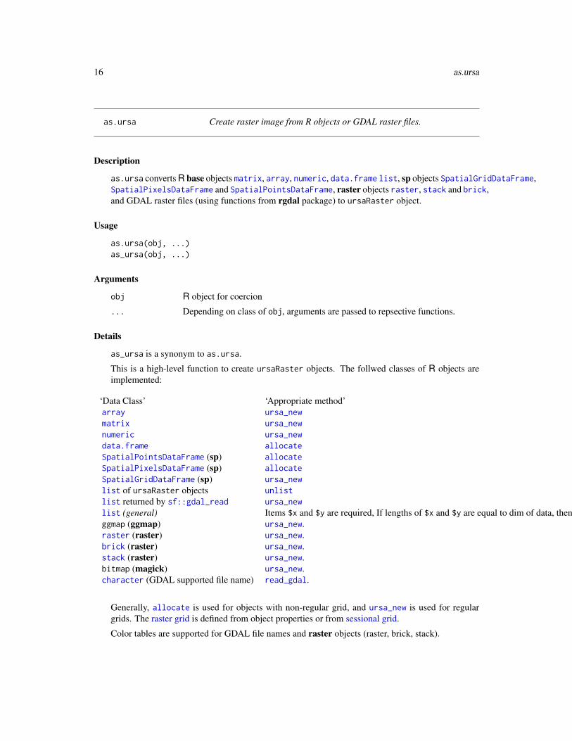
as.ursa Create raster image from R objects or GDAL raster files.

Description

as.ursa converts R base objects matrix, array, numeric, data.frame list, sp objects SpatialGridDataFrame,SpatialPixelsDataFrame and SpatialPointsDataFrame, raster objects raster, stack and brick,and GDAL raster files (using functions from rgdal package) to ursaRaster object.

Usage

as.ursa(obj, ...)as_ursa(obj, ...)

Arguments

obj R object for coercion

... Depending on class of obj, arguments are passed to repsective functions.

Details

as_ursa is a synonym to as.ursa.

This is a high-level function to create ursaRaster objects. The follwed classes of R objects areimplemented:

‘Data Class’ ‘Appropriate method’array ursa_newmatrix ursa_newnumeric ursa_newdata.frame allocateSpatialPointsDataFrame (sp) allocateSpatialPixelsDataFrame (sp) allocateSpatialGridDataFrame (sp) ursa_newlist of ursaRaster objects unlistlist returned by sf::gdal_read ursa_newlist (general) Items $x and $y are required, If lengths of $x and $y are equal to dim of data, then allocate, else: 1) raster grid is defined from $x and $y, 2) ursa_new is called.ggmap (ggmap) ursa_new.raster (raster) ursa_new.brick (raster) ursa_new.stack (raster) ursa_new.bitmap (magick) ursa_new.character (GDAL supported file name) read_gdal.

Generally, allocate is used for objects with non-regular grid, and ursa_new is used for regulargrids. The raster grid is defined from object properties or from sessional grid.

Color tables are supported for GDAL file names and raster objects (raster, brick, stack).

as.ursa 17

For ENVI *.hdr Labelled Raster Files there are alternatives:

1. Read object with GDAL (read_gdal);

2. Read object without GDAL (read_envi).

Value


Author(s)


Examples

session_grid(NULL)a1 <- as.ursa(volcano)print(a1)display(a1)

session_grid(NULL)b <- ursa_dummy(mul=1/16,bandname=format(Sys.Date()+seq(3)-1,"%A"))print(b)

c1 <- b[[1]] ## equal to 'c1 <- as.matrix(b[1],coords=TRUE)'str(c1)b1a <- as.ursa(c1)print(c(original=b[1],imported=b1a))print(c(projection.b1a=ursa_proj(b1a)))session_grid(NULL)b1b <- as.ursa(c1$z)print(b1b)print(c(projection.b1b=ursa_proj(b1b)))

c2 <- as.data.frame(b)str(c2)session_grid(NULL)b2a <- as.ursa(c2)print(b2a)

session_grid(NULL)attr(c2,"crs") <- NULLb2b <- as.ursa(c2)print(b2b)print(ursa_grid(b2b))

c3 <- unclass(as.matrix(b,coords=TRUE))str(c3)session_grid(b)b3a <- as.ursa(c3)print(b3a)print(ursa_grid(b3a))

18 bandname

session_grid(NULL)b3b <- as.ursa(c3)print(b3b)print(ursa_grid(b3b))

c4 <- as.array(b)str(c4)session_grid(b)b4a <- as.ursa(c4)print(b4a)print(ursa_grid(b4a))session_grid(NULL)b4b <- as.ursa(c4)print(b4b)print(ursa_grid(b4b))

n <- 20c5 <- data.frame(y=runif(n,min=1000000,max=5000000)

,x=runif(n,min=-3000000,max=1000000),value=runif(n,min=0,max=10))

print(head(c5))session_grid(b)b5a <- as.ursa(c5)print(b5a)display(b5a)session_grid(NULL)b5b <- as.ursa(c5)print(b5b)display(b5b)

b6 <- as.ursa(system.file("pictures/erdas_spnad83.tif",package="rgdal"))print(b6)display(b6,coast=FALSE,col="orange")

## package 'raster' is required -- beginif (requireNamespace("raster")) {

r <- raster::brick(system.file("external/rlogo.gri",package="raster"))print(r)b7 <- as.ursa(r)ursa_proj(b7) <- ""print(b7)display_rgb(b7)}

## package 'raster' is required -- end

bandname Band names for raster image.

Description

bandname (names) returns names of bands for object of class ursaRaster or existing ENVI labelled*.hdr file. bandname<- (names<-) sets names of bands for object of class ursaRaster.

bandname 19

Usage

bandname(x)bandname(x) <- value

## S3 method for class 'ursaRaster'names(x)

## S3 replacement method for class 'ursaRaster'names(x) <- value

Arguments

x Object of class ursaRaster. In the bandname function it is allowed to specifycharacter ‘ENVI labelled *.hdr’ file name.

value Character of length the same length of number of bands of x

Details

names is a synonym for bandname. names<- is a synonym for bandname<-

Value

For bandname and names, character vector.

For bandname<- and names<-, updated object of class ursaRaster.

Author(s)


See Also

nband

Examples

session_grid(NULL)a1 <- pixelsize()a2 <- c("Band 1"=a1,Band2=a1/2,sqrt=sqrt(a1),NA)print(a2)print(bandname(a2))bandname(a2)[1:2] <- c("Original","Half")print(a2)print(bandname(a2))

20 band_group

band_group Extract certain statistics of each band.

Description

Function from this band.* list returns required statistics for each band.

Usage

band_mean(obj)band_sd(obj)band_sum(obj)band_min(obj)band_max(obj)band_n(obj)band_nNA(obj)

Arguments

obj Object of class ursaRaster.

Details

• band_mean returns mean value.

• band_sd returns value of standard deviation with n-1 denominator.

• band_sum returns sum of values.

• band_min returns minimal value.

• band_max returns maximal value.

• band_n returns number of non-NA pixels.

• band_nNA returns number of NA pixels.

Value

Named vector of numerical or integer values. Band names are used for naming.

Note

Currently, implementation is not optimal, because firstly bundle of statistics is computed usingband_stat function, and then required statistics is extracted.

Author(s)


See Also

band_stat

band_stat 21

Examples

session_grid(NULL)a <- ursa_dummy()print(a)print(a<80)print(class(a))a[a<80]a[a<80] <- NAb1 <- band_stat(a)print(b1)b2.n <- band_n(a)str(b2.n)b2.mean <- band_mean(a)print(b1$mean)print(b2.mean)print(b1$mean-b2.mean)

band_stat Computes statistics for each band of raster.

Description

For each band of ursaRaster object, band_stat returns certain statistics (mean, sd, sum, min, max,number of non-NA pixels, number of NA pixels). Regarding to each band, it is global operations ofmap algebra.

Usage

band_stat(x, grid = FALSE, raw = FALSE)

Arguments

x Object of class ursaRaster.

grid Logical. If TRUE then metadata are returned instead of statistics. Default isFALSE

raw Logical. For the case of raster values are categories, if raw=TRUE, then func-tion returns statistics of categories; if raw=FALSE and names of categories canbe transformed to numerical values, then function returns statistics for decate-gorized values. Default is FALSE.

Details

If raster values are not in memory or grid=TRUE then ursa_info is returned.

Generic function print for object of class ursaRaster uses returned value of band_stat functionwith formatted columns.

Statistics is computed for omitted NA values.

22 blank

Value

data.frame. Row names are indices of bands. Column names are:

name Band name.

mean Mean value.

sd Value of standard deviation with n-1 denomination.

sum Sum of values.

min Minimal value.

min Maximal value.

n Number of non-NA pixels.

nNA Number of NA pixels.

Author(s)


See Also

Columns extraction from returned data frame is in the group of band.* functions.

Examples

session_grid(NULL)s <- substr(as.character(sessionInfo()),1,48)a <- reclass(ursa_dummy(mul=1/2,bandname=s),ramp=FALSE)band_stat(a,grid=TRUE)b2 <- band_stat(a)b3 <- band_stat(a,raw=TRUE)str(b2)str(b3)print(b2)print(a) ## 'print.ursaRaster' uses 'band_stat'print(a,raw=TRUE)

blank Does any band contain no information?

Description

Set of functions for checking is any or all bands have no data, and for retrieving indices for non-databands.

Usage

band_blank(obj, ref = c("any", "0", "NA"), verbose = FALSE)

ursa_blank(obj, ref)

blank 23

Arguments

obj Object of class ursaRaster

ref Character. Definition criteria, what is blank mean. If value "0", then blank isdetected, if all values are 0. If value "NA", then blank is detected, if all valuesare NA. Default value is "NA": both NA and 0 are flags of blank. Non-charactervalues are coerced to character.

verbose Logical. Value TRUE provides progress bar. Default is FALSE.

Details

It is defined locally that if all values of band are NA or 0 (see description to argument ref), thensuch band is blank. The fact is ursa_new create new object in memory with default values NA,but create_envi writes zeros to disk quick. It is decided to consider both these cases as blank.Function band_blank checks blanks for each band of image. If all bands are blank then functionursa_blank returns TRUE.

Value

Function ursa_blank returns logical value of length 1.

Function band_blank returns logical value of length nband(obj).

Author(s)


See Also

is.na returns object of class ursaRaster; it is mask of cells, which have NA value.

Examples

session_grid(NULL)a <- ursa_new(bandname=c("first","second","third","fourth"))ursa_value(a,"first") <- 0 ## 'a[1] <- 1' works, but it is slowprint(ursa_blank(a))a[3] <- pixelsize()a[4] <- a[3]>625print(a)print(band_blank(a))print(which(band_blank(a)))print(ursa_blank(a))

24 c

c Combine bands into raster brick.

Description

This function is an instrument for appending bands or for reorganizing bands.

Usage

## S3 method for class 'ursaRaster'c(...)

Arguments

... Objects of class ursaRaster or coerced to class ursaRaster. First argumentshould be the object of class ursaRaster. The objects in the sequence can benamed.

Details

You may use this function to assign new bandname for single-band raster: objDst <-c('Relativedensity'=objSrc)

Use also ’Extract’ operator [ ] to reorganize band sequence.

The returned object can be interpreted as a brick in the notation of package raster. To producestack just call list or ursa_stack.

Value

ursaRaster object.

Author(s)


See Also

ursa_brick converts list of ursaRaster objects (stack) to a singe multiband ursaRaster object(brick).

Examples

session_grid(NULL)session_grid(regrid(mul=1/16))a1 <- ursa_dummy(nband=2)names(a1) <- weekdays(Sys.Date()+seq(length(a1))-1)a2 <- ursa_dummy(nband=2)names(a2) <- names(a1)print(a1)

chunk 25

print(a2)a3 <- a1[1]print(names(a3))a4 <- c(today=a3)print(names(a4))print(b1 <- c(a1,a2))print(b2 <- c(a1=a1))print(b3 <- c(a1=a1,a2=a2))print(b5 <- c(a1=a1,a2=a2[1]))print(b4 <- c(a1,'(tomorrow)'=a1[2])) ## raster appendprint(b6 <- c(a1,50))

chunk Get indices for partial image reading/writing

Description

In the case of ’Cannot allocate vector of size ...’ error message chunk_band returns list of bandsindices, which are suitable for allocation in memory at once, chunk_line returns list of lines (rows)indices, which are suitable for allocation in memory at once. chunk_expand is used to expand linesindices and can by applied in focal functions.

Usage

chunk_band(obj, mem = 100, mul = 1)chunk_line(obj, mem = 100, mul = 1)chunk_expand(ind, size = 3)

Arguments


mem Numeric. Memory size in GB, which is suitable for allocation.

mul Numeric. Expansion or reduction factor (multiplier) of default value of memoryallocation.

ind Integer. Line indices.

size Integer. Size of focal window.

Value

chunk_band returns list with sequences of bands

chunk_line returns list with sequences of lines

chunk_expand returns list:

src expanded set if line indices

dst matching of source indices in the expanded set

26 close

Author(s)


Examples

## 1. Prepare datasession_grid(NULL)fname <- ursa:::.maketmp(2)a <- create_envi(fname[1],nband=3,ignorevalue=-99)for (i in seq(nband(a)))

a[i] <- pixelsize()^(1/i)close(a)rm(a)

## 2. Reada <- open_envi(fname[1])chB <- chunk_band(a,2)str(chB)for (i in chB)

print(a[i])chL <- chunk_line(a,2.5)str(chL)for (j in chL)

print(a[,j])

## 3. Filtering with partial readingb <- create_envi(a,fname[2])fsize <- 15for (j in chL) {

k <- chunk_expand(j,fsize)b[,j] <- focal_mean(a[,k$src],size=fsize)[,k$dst]

}d1 <- b[]

## 4. Filtering in memoryd2 <- focal_mean(a[],size=fsize)close(a,b)envi_remove(fname)print(d1-d2)print(round(d1-d2,4))

close Close connections for files with data

Description

close() for ursaRaster object closes connection for opened file using inheritted function base::close.Function close_envi() closes opened connection for ENVI binary file.

codec 27

Usage

## S3 method for class 'ursaRaster'close(...)

close_envi(...)

Arguments

... Object or sequence of objects of class ursaRaster.

Value

NULL

Author(s)


See Also

close of base package

Examples

session_grid(NULL)a <- create_envi()fname <- a$con$fnamemessage(paste("Created file",dQuote(basename(fname)),"will be deleted."))print(dir(pattern=basename(envi_list(fname))))close(a)invisible(envi_remove(fname))

codec Reduce and restore dimenstions for sparse data matrix

Description

compress reduces dimension of source image matrix and assigns indices. decompress uses indicesfor expansion of reduced image matrix.

Usage

decompress(obj)compress(obj)

Arguments


28 colorize

Details

After masking, vectorization of lines, points and small polygons image matrix is often sparse. Com-pressing (compress) is an option to reduce object size in memory. Decompressing (decompress)restore original data matrix.

Value


Note

Currently, usage of compressed image matrix is limited. Spatial filtering (e.g. focal_mean) doesnot operate with compressed data.

Author(s)


Examples

session_grid(NULL)b <- as.data.frame(pixelsize())b <- subset(b,x>1000000 & x<2000000 & y>3000000 & y<4000000)a1 <- as.ursa(b)print(a1)print(object.size(a1))a2 <- compress(a1)print(a2)print(object.size(a2))a3 <- decompress(a2)print(a3)print(object.size(a3))print(identical(a1,a3))

colorize Create color table

Description

colorize assigns color table to raster image.

Usage

colorize(obj, value = NULL, breakvalue = NULL, name = NULL, pal = NULL, inv = NA,stretch = c("default", "linear", "equal", "mean", "positive",

"negative", "diff", "category", "julian", "date", "time","slope", "conc", "sd", "significance", "bathy","grayscale", "greyscale", ".onetoone"),

colorize 29

minvalue = NA, maxvalue = NA, byvalue = NA, ltail = NA, rtail = NA, tail = NA,ncolor = NA, nbreak = NA, interval = 0L, ramp = TRUE, byte = FALSE,lazyload = FALSE, reset = FALSE, origin = "1970-01-01" ,format = "",alpha = "", colortable = NULL, verbose = FALSE, ...)

Arguments

obj ursaRaster object or one-dimension numeric vector.

value Numeric. Values to be assigned to categories.

breakvalue Numeric. Values to be assigned to intervals.

name Character. Names of categories.

pal Function or character. If function then value should corresponded to function,which creates a vector of colors. If character then values should correponded toR color names or hexadecimal string of the form "#RRGGBB" or "#RRGGB-BAA".

inv Logical. Invert sequence of colors.

stretch Character. Either kind of value transformation ("linear","equal") or pre-defined options with palette specification ("positive","data","significance",etc)

minvalue Numeric. Lower range limit.

maxvalue Numeric. Upper range limit.

byvalue Numeric. Increment of the sequence from minvalue to maxvalue.

ltail Numeric. Partition of omitted values at left tail.

rtail Numeric. Partition of omitted values at right tail.

tail Numeric. Partition of omitted values at both tail. If length of tail is 2 then leftand right tails may differ.

ncolor Numeric or interer. Number of desired colors (or categories)

nbreak Numeric or interer. Number of desired separators between colors.

interval Integer. How to underwrite categories? Use direct

ramp Logical. Is color ramp required?

byte Logical. Forcing to produce color table for storage in byte format (not morethan 255 colors). Default is FALSE.

lazyload Logical. If FALSE then raster is reclassified to categories. If TRUE then colortable is created without any change to source raster. Default is FALSE.

reset Logical. If TRUE and source raster has color table, then this color table is de-stroyed, and new one is created. Default is FALSE.

origin Character. Origin for stretch="date" (passed to function as.Date) and stretch="time"(passed to function as.POSIXct). See desription of orogin in respective func-tions. Default is "1970-01-01".

format Character. Format date/time objects for arguments stretch with values "date","time", or "julian". Default is "" (character of length 0).

30 colorize

alpha Character or numeric. The characteristics of transparency. If character, thenhexadecimal values between "00" and "FF" are allowed, and then coerced tonumeric value between 0 and 255. If numeric, and 0 <= alpha <= 1, then alphais multiplied to 255. alpha=0 means full transparency, alpha=255 means fullopacity. Default is ""; if palette has no alpha channel, then alpha is assign to"FF".

colortable Object of class ursaColorTable or object of class ursaRaster with color ta-ble. Reference color table. Is specified, then all other arguments are ignored,expexted lazyload. Default is NULL (unspecified).

verbose Logical. Some output in console. Primarily for debug purposes.

... If pal is a function, and argument names are in the format "pal.*" then prefix"pal." is omitted, and the rest part is used for argument names, which are passedto pal function.

Details

colortable is designed to prepare pretty thematic maps.

Color rampimg (ramp=TRUE) is not quick in computatons and has no effective labelling. It is in-toduced to visualize non-thematic maps, and it is assumed that labeling can be omitted for suchmaps.

The labelling implementation is based on some improvements of pretty function. The notation ofintervals is mixed by brackets and comparative symbols, for example: "<=1.5","(1.5,2.5]","(2.5,3.5]",">3.5"

Reserved values for interval:

• 0L or FALSE - no interlavs. Values are interpreted as category, even if they are in non-nominalscale

• 1L or TRUE - each category corresponds to interval. The low limit of lowest category is -Inf.The high limit of highest category is +Inf

• 2L - different implementation of interval=1. In some cases may relult more pretty labeling.If breaks is numerical vector and colors has zero length, then it is assumed interal scaling,and interval=1L is assigned to unspecified interval

Finite values of extreme intervals are neccessary sometimes, however this option is not imple-mented currently

Keywords for stretch to create pre-defined color tables:

• "positive" - lower limit is 0. Palette is "Oranges"

• "negative" - higher limit is 0. Palette is "Purples"

• "grayscale","greyscale" - palette is "Greys". Usually used for raw satellite images.

• "mean" - designed for common thematic maps and for averaged map across set of maps.Palette is "Spectral"

• "sd" - designed for spatial mapping of standard deviation across set of maps. Palette is "Yl-GnBu"

• "diff" - diverge palette "RdBu". Absolute values of lower and upper limits are equal, zero isin the middle of palette. Designed for anomaly maps.

colorize 31

• "slope" - is similar to diff but without extreme colors, which are reserved for contouring ofstatistically significant areas.

• "significance" - desiged to illustrate statistically significant areas of slope. The realisationis colortable(obj,value=c(-0.999,-0.99,-0.95,-0.9,-0.5,+0.5,+0.9,+0.95,+0.99,+0.999),interval=1L,palname="RdBu")

• "category" - Values are interpreted in nominal scale. Palette is based on random colors from"Pairs" palette.

• "conc" - designed for visualization of sea ice concentration data, which have lower limit 0and higher limit 100. Palette is "Blues"

• "bathy" - designed for ocean depth (bathymetry) maps. Internally colorize(obj,stretch="equal",interval=1L,palname="Blues",inv=TRUE)is used to detect the crossing from shelf waters to deep water basin. Better practice is to dosecond step with manual specification of value argument.

• "internal" - continuous colors, designed for conversion to greyscale with keeping of inten-sities.

• "default" - allowing to detect stretch by intuition, without any strong mathematical criteria

It is allowed manual correction of labels using followed code example: names(ursa_colortable(x))<-c("a<=0","0<a<=1","a>1")

Value

Object of class ursaRaster with named character vector of item $colortable

Author(s)


See Also

ursa_colortable, ursa_colortable<-

Examples

session_grid(NULL)a <- pixelsize()-350print(a)b1 <- colorize(a,ramp=FALSE)print(ursa_colortable(b1))b2 <- colorize(a,interval=1,stretch="positive",ramp=FALSE)print(ursa_colortable(b2))b3 <- colorize(a,interval=2,stretch="positive",ramp=FALSE)print(ursa_colortable(b3))b4 <- colorize(a,value=c(150,250),interval=1)print(ursa_colortable(b4))names(ursa_colortable(b4)) <- c("x<=150","150<x<=250","x>250")print(ursa_colortable(b4))display(b4)

32 colortable

colortable Color Tables of raster images.

Description

Manipulation with color tables of raster images.

Usage

## S3 method for class 'ursaColorTable'print(x, ...)

## S3 method for class 'ursaColorTable'x[i]

ursa_colortable(x)

ursa_colortable(x) <- value

ursa_colorindex(ct)

## S3 method for class 'ursaColorTable'names(x)

## S3 replacement method for class 'ursaColorTable'names(x) <- value

Arguments

x ursaRaster object.

ct ursaColorTable object with or without indexing.

value Named character vector. In Replacement functions:For ursa_colortable(): values are colors in “#RRGGBB” notation or R colornames (colors). names(value) are names of categories.For names(): values are names of categories. If length of names is n-1, wheren is length of colors, then intervaling is assumed, and codevalue are assign tointerval breaks.

i Integer vector. Indices specifying elements to extract part (subset) of color table.

... passing to generic print. Currently not used.

Details

The example of the class structure

colortable 33

Class 'ursaColorTable' Named chr [1:4] "#313695" "#BCE1EE" "#FDBE70" "#A50026"..- attr(*, "names")= chr [1:4] "<= 450" "(450;550]" "(550;650]" "> 650"

It is recommended to use ursa_colortable and ursa_colortable<- instead of colortable andcolortable<-. ursa_colortable and colortable are synonyms. ursa_colortable<- andcolortable<- are synonyms too. Package raster contains colortable and colortable<- func-tions. colortable and colortable<- will be remove from this package if the case of frequentjoint use of both packages.

If color tables describe continuous and non-intersecting intervals, then print gives additional lineof extracted breaks.

Value

ursa_colortable returns value of $colortable element if ursaRaster object.

ursa_colortable<- returns ursaRaster object with modified $colortable element.

Class of $colortable element is “ursaColorTable”. This is named character vector, where namesare categories, and values are “#RRGGBB” or R color names.

Extract function [] for ursaColorTable object returns object of class ursaColorTable.

Extract function names for ursaColorTable object returns character vector (names of categories).

Replace function names<- for ursaColorTable object returns ursaColorTable with changed namesof categories.

ursa_colorindex returns index (if presents) for ursaColorTable object.

Color tables are written to ENVI header file.

Warning

If colors are specified as R color names, then slow down may appear.

Author(s)


See Also

colorize

Examples

session_grid(NULL)print(methods(class="ursaColorTable"))

a <- pixelsize()print(a)b1 <- colorize(a,value=c(400,500,600,700),interval=FALSE)b2 <- colorize(a,value=c(450,550,650) ,interval=TRUE)display(list(b1,b2))print(is.ursa(a,"colortable"))print(is.ursa(b1,"colortable"))

34 commonGeneric

print(is.ursa(b2,"colortable"))print(ursa_colortable(a))print(ursa_colortable(b1))print(ursa_colortable(b2))ursa_colortable(b2) <- c("Low"="darkolivegreen1"

,"Moderate"="darkolivegreen2","High"="darkolivegreen3","errata"="darkolivegreen4")

print(ursa_colortable(b2))names(ursa_colortable(b2))[4] <- "Polar"print(ursa_colortable(b2))display(b2)

commonGeneric Some generic functions for ursaRaster class.

Description

Set of generic functions, implemented for objects of ursaRaster class.

Usage

## S3 method for class 'ursaRaster'duplicated(x, incomparables = FALSE, MARGIN = 2, fromLast = FALSE, ...)

## S3 method for class 'ursaRaster'diff(x, lag = 1, differences = 1, ...)

Arguments

x Object of ursaRaster class

incomparables Passed to S3 method duplicated for class matrix.

MARGIN Overwitten to value 2. Passed to S3 method duplicated for class matrix.

fromLast Passed to S3 method duplicated for class matrix.

lag Passed to default S3 method diff.

differences Passed to default S3 method diff.

... Other arguments, which are passed to the respective S3 method.

Value

duplicated(): logical of length equal to number of bands.

diff(): ursaRaster object.

Author(s)


compose_close 35

See Also

duplicated, diff,

Examples

a <- ursa_dummy(5)a[3] <- a[2]aduplicated(a)diff(a)

compose_close Finish plotting

Description

Function compose_close does followed tasks: 1) completes all unfinsished actions before shuttingdown graphical device, 2) cuts extra margins, and 3) opens resulted PNG file in the associatedviewer.

Usage

compose_close(...)

## non-public.compose_close(kind = c("crop2", "crop", "nocrop"),

border = 5, bpp = 0, execute = TRUE, verbose = FALSE)

Arguments

... Set of arguments, which are recognized via their names and classes, and thenpassed to .compose_close:

Pattern (compose_close) Argument (.compose_close)(^$|crop|kind) kind(border|frame) borderbpp bpp(render|execute|view|open) executeverb(ose)* verbose

kind Character keyword for cutting of excess white spaces. If kind="nocrop" thenthere is no cut. If kind="crop" then only outer margins are cutted. If kind="crop2"then all outer margins and inner white spaces (e.g., between color bar panel andtext caption) are cutted.

border Non-negative integer. Number of pixels for margins, which are not cropped.Default is 5L.

36 compose_close

bpp Integer. Bits per pixel for output PNG file. Valid values are 0L, 8L, 24L. Ifbpp=0L, then 8 bpp is used for "windows" type of PNG device, and 24 bppis used for "cairo" type of PNG device. The type of device is specified incompose_open function.

execute Logical. Should created PNG file be opened in the associated external programfor viewing graphical files? Default is TRUE.

verbose Logical. Value TRUE provides some additional information on console. Defaultis FALSE.

Details

The cut manipulations (crop="crop" or crop="crop2") are implemented using readPNG and writePNGfunctions of package png. These fuctions have limitations in the memory allocation.

Function compose_close clears all internal graphical options, specified during compose_open ex-ecuting.

Some parameters are specified in compose_open: weather output PNG file will be removed afteropening (logical delafter), or what is the time of waiting for file opening and next removing(numerical wait in seconds).

Value

Function returns NULL value.

Warning

Currenty, execute=TRUE is implemented for Windows platform only using construction R CMD open \emph{fileout}.

Author(s)


Examples

session_grid(NULL)a <- ursa_dummy(nband=6,min=0,max=255,mul=1/4)

## exam 1compose_open()compose_close()

## exam 2compose_open(a)compose_close()

## exam 3compose_open("rgb",fileout="tmp1")compose_plot(a[1:3])compose_close(execute=FALSE)Sys.sleep(1)a <- dir(pattern="tmp1.png")

compose_design 37

print(a)file.remove(a)

compose_design Organize multi-panel layout with images and color bars.

Description

compose_design prepares scheme for layout of images and color bars.

Usage

compose_design(...)

Arguments

... Set of arguments, which are recognized via their names and classes:

obj Object of class ursaRaster or list of objects of class ursaRaster or NULL.Default is NULL. Used to detect panel layout and coordinate reference sys-tem.

layout Integer of length 2 or NA. Layout matrix has dimensionsc(nr,nc), wherenr is number of rows, and nc is number of columns. If layout=NA thenlayout matrix is recognized internally using number of bands of obj andargument ratio. If layout=NA and obj=NULL then matrix c(1,1) is used.

byrow Logical. The order of filling of layout matrix. Default is TRUE. If byrow=TRUEthen matrix is filled by rows (from top row, consequently from left elementto right element, then next row). If byrow=FALSE then matrix is filled bycolumns.

skip Positive integer of variable length. Default in NULL (length is zero). In-dices of panels in the layout matrix, which are not used.

legend The descripition of rules how color bars (legends) or panel captions arelocated in the layout. It is the list of embedded lists of two elements, whichdescribe the color bars position in the layout. of Default is NA, it meansusing of internal rules. If legend=NULL then no plotting of color bars. Iflegend is positive integer in the range 1L:4L, then sinlge color bar is usedand legend’s side is corresponded to margins of R graphic system.

side Positive integer 1L, 2L, 3L, or 4L. Default is NA. Simplification of color barposition in the case that single color bar is used. The value is correspondedto margins of R graphic system. The synonym of integer value of legend.

ratio Positive numeric. The desired ratio of layout sides (width per height). Iflayout=NA then the dimensions of layout matrix are defined internally toget the given ratio of layout’s width per height. The default is (16+1)/(9+1)in the assumtion of optimal filling on the usual 16:9 screens.

38 compose_design

Details

Function compose_design extracts and validates required arguments from a list of parameters(three-dots construct) and passes them to internal function .compose_design.

Argument legend is a list or coerced to a list. The length of this list is equal to number of colorbars; each item describes certain color bar. This desctiption is a list again with two elements, whichdesribes the position of color bar in relation to main panels of images.

If argument legend is in interval 1L:4L then it is interpreted as argument side in functions axis,mtext. Argument side in function compose_design plays the same role. It is introduced forconsistency with R graphic system.

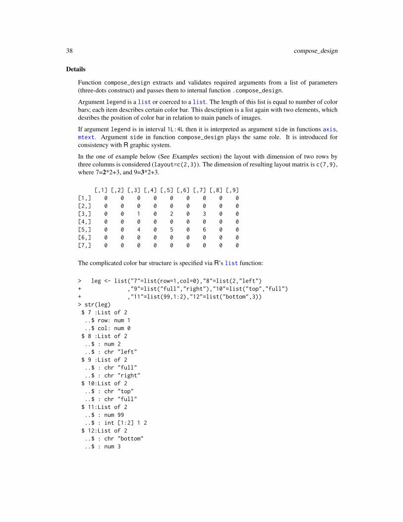
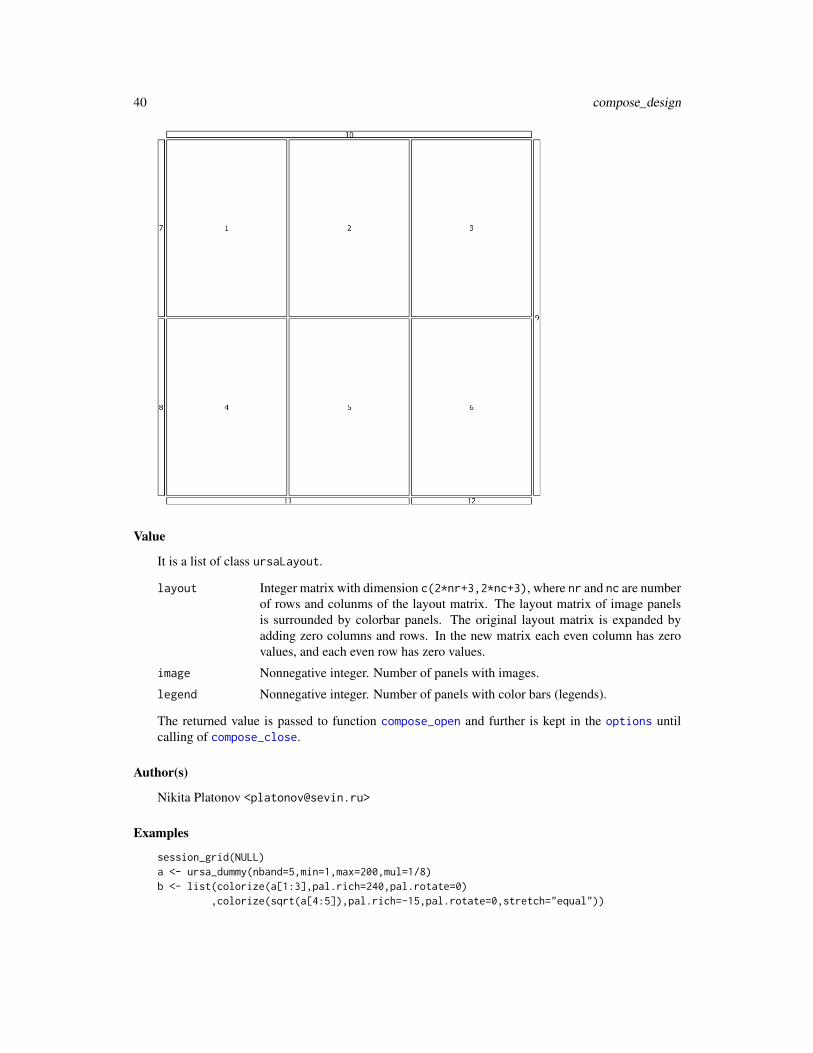
In the one of example below (See Examples section) the layout with dimension of two rows bythree columns is considered (layout=c(2,3)). The dimension of resulting layout matrix is c(7,9),where 7=2*2+3, and 9=3*2+3.

[,1] [,2] [,3] [,4] [,5] [,6] [,7] [,8] [,9][1,] 0 0 0 0 0 0 0 0 0[2,] 0 0 0 0 0 0 0 0 0[3,] 0 0 1 0 2 0 3 0 0[4,] 0 0 0 0 0 0 0 0 0[5,] 0 0 4 0 5 0 6 0 0[6,] 0 0 0 0 0 0 0 0 0[7,] 0 0 0 0 0 0 0 0 0

The complicated color bar structure is specified via R’s list function:

> leg <- list("7"=list(row=1,col=0),"8"=list(2,"left")+ ,"9"=list("full","right"),"10"=list("top","full")+ ,"11"=list(99,1:2),"12"=list("bottom",3))> str(leg)$ 7 :List of 2..$ row: num 1..$ col: num 0$ 8 :List of 2..$ : num 2..$ : chr "left"$ 9 :List of 2..$ : chr "full"..$ : chr "right"$ 10:List of 2..$ : chr "top"..$ : chr "full"$ 11:List of 2..$ : num 99..$ : int [1:2] 1 2$ 12:List of 2..$ : chr "bottom"..$ : num 3

compose_design 39

Here, six color bars are specified. It is a list of six lists (sub-lists). First item of sub-list is rownumber, and the second one is column number. Integers can be replaces by character keywords.

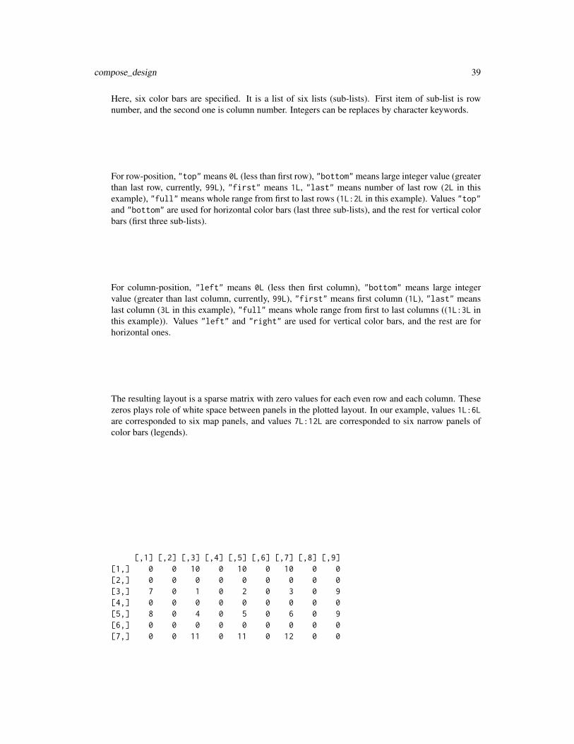
For row-position, "top" means 0L (less than first row), "bottom" means large integer value (greaterthan last row, currently, 99L), "first" means 1L, "last" means number of last row (2L in thisexample), "full" means whole range from first to last rows (1L:2L in this example). Values "top"and "bottom" are used for horizontal color bars (last three sub-lists), and the rest for vertical colorbars (first three sub-lists).

For column-position, "left" means 0L (less then first column), "bottom" means large integervalue (greater than last column, currently, 99L), "first" means first column (1L), "last" meanslast column (3L in this example), "full" means whole range from first to last columns ((1L:3L inthis example)). Values "left" and "right" are used for vertical color bars, and the rest are forhorizontal ones.

The resulting layout is a sparse matrix with zero values for each even row and each column. Thesezeros plays role of white space between panels in the plotted layout. In our example, values 1L:6Lare corresponded to six map panels, and values 7L:12L are corresponded to six narrow panels ofcolor bars (legends).

[,1] [,2] [,3] [,4] [,5] [,6] [,7] [,8] [,9][1,] 0 0 10 0 10 0 10 0 0[2,] 0 0 0 0 0 0 0 0 0[3,] 7 0 1 0 2 0 3 0 9[4,] 0 0 0 0 0 0 0 0 0[5,] 8 0 4 0 5 0 6 0 9[6,] 0 0 0 0 0 0 0 0 0[7,] 0 0 11 0 11 0 12 0 0

40 compose_design

Value

It is a list of class ursaLayout.

layout Integer matrix with dimension c(2*nr+3,2*nc+3), where nr and nc are numberof rows and colunms of the layout matrix. The layout matrix of image panelsis surrounded by colorbar panels. The original layout matrix is expanded byadding zero columns and rows. In the new matrix each even column has zerovalues, and each even row has zero values.

image Nonnegative integer. Number of panels with images.

legend Nonnegative integer. Number of panels with color bars (legends).

The returned value is passed to function compose_open and further is kept in the options untilcalling of compose_close.

Author(s)


Examples

session_grid(NULL)a <- ursa_dummy(nband=5,min=1,max=200,mul=1/8)b <- list(colorize(a[1:3],pal.rich=240,pal.rotate=0)

,colorize(sqrt(a[4:5]),pal.rich=-15,pal.rotate=0,stretch="equal"))

compose_legend 41

cl1 <- compose_design(layout=c(2,3),byrow=TRUE,legend=NULL)print(cl1)compose_open(cl1)compose_close()

cl2 <- compose_design(layout=c(2,3),byrow=FALSE,legend="left")print(cl2$layout)compose_open(cl2)compose_close()

cl3 <- compose_design(a,side=2)print(cl3)compose_open(cl3)compose_close()

cl4 <- compose_design(b)print(cl4)## to avoid over-time during example check -- begincompose_open(cl4)compose_plot(b,decor=FALSE,las=2)compose_close("nocrop")

## to avoid over-time during example check -- end

cl5 <- compose_design(b,byrow=FALSE,skip=3,legend=list(list("full","left"),list(1:2,"right")))

compose_open(cl5)compose_plot(b,decor=FALSE)compose_close("nocrop")

leg <- list(list(1,0),list(2,"left"),list("full","right"),list("top","full"),list(99,1:2),list("bottom",3))

str(leg)cl6 <- compose_design(layout=c(2,3),skip=NA,legend=leg)print(cl6)compose_open(cl6,scale=3,pointsize=16)compose_close("nocrop")

compose_legend Plot colorbars or marginal texts.

Description

compose_legend recognizes color tables and characters among arguments and passes them to suit-able functions for plotting on margins outside of panel area.

Usage

compose_legend(...)

42 compose_legend

Arguments

... If first argument is a list, then either ursaColorTable or character objects aredetected in this list. ursaColorTable can be extracted from ursaRaster (ifpresents). Other objects are coerced to character.If first argument is ursaColorTable or ursaRaster with color tables, then otherarguments are interpreted as color tables. If coercion to color table is impossible,the coersion is to character.legend_colorbar is called for objects of class ursaColorTable. legend_mtextis called for objects of class ursaColorTable. If first argument is a list, thenother arguments are passed to respective function calls.

Details

Named list in the first argument is allowed or named vectors are allowed if first argument is not alist. For legend_colorbar name of object can be used as an argument units.

This function is designed to make plot on moderate level of usage with the followed construction:

compose_open(...)compose_panel(...)compose_legend(...)compose_close(...)

Function compose_panel returns list of color tables of plotted rasters, and followed sequence isavailable:

ct <- compose_panel(a)compose_legend(ct) # or, if 'a' has color tables, then 'compose_legend(a)'

Value

NULL

Author(s)


See Also

legend_colorbar

legend_mtext

Examples

session_grid(NULL)b <- lapply(as.list(ursa_dummy(2)),colorize)cd <- compose_design(layout=c(1,2),legend=list(list(1,"left"),list(1,"right")

,list("top","full"),list("bottom",1)))for (i in 1:4) {

compose_open(cd,dev=i==1)

compose_open 43

ct <- compose_panel(b,decor=FALSE)if (i==2)

compose_legend(ct)else if (i==3)

compose_legend(ct[[1]],'Tomorrow'=b[[2]],top="This is example of legend composition",format(Sys.Date(),"(c) %Y"))

else if (i==4)compose_legend(c(ct,"top","bottom"),units=c("left","right"))

compose_close()}

compose_open Start displaying

Description

compose_open create plot layout and open PNG graphic device.

Usage

compose_open(...)

Arguments

... Set of arguments, which are recognized via their names and classes:

mosaic Layout matrix or reference object to produce layout matrix. It is per-mitted to do not use name for this argument. Multiple types of argumentare allowed: 1) object of class ursaRaster, 2) list of ursaRaster objects(raster stack), 3) object of class ursaLayout from function compose_design,4) character keyword or 5) missing. Default is NA.

fileout Character. Name for created PNG file. If absent ("") then temporalfile is created and removed in wait seconds after opening in the associatedexternal viewer. Default is absent ("").

dpi Positive integer. Dots (or pixels) per inch (DPI). The nominal resolutionof created PNG file. Default is 96L. The same as res argument in the pngfunction.

pointsize Positive integer. The pointsize of plotted text as it is applied in thepng function. Default is NA. If pointsize=NA then it is taken value 16Lmultiplied to relative DPI (dpi/96). In the case of unspecified scale andpointsize the size of text is defined internally.

scale Positive numeric or character. The scale factor applied to dimensionsof original raster. Default is NA. If scale is unspecified (scale=NA), thenscale is defined internally for intuitively better fitting in HD, FHD displays(single-panelled layout 900x700). If scale is character (e.g., "8000000","1:8000000") then dimensions of image panels are defined using "one cen-timeter of map is corresponded to 8000000 centimeres of site" rule.

44 compose_open

width Positive numeric or character. The desired width of each panel of multi-panel layout. If width is numeric, then units are pixels. If width is charac-ter (e.g., "12.5", "12.5 cm", "12.5cm") then units are centimeters in agree-ment with dpi argument. Default is NA. If width is unspecified (width=NA)then value 900 is used for single panelled layout.

height Positive numeric or character. The desired height of each panel of mul-tipanel layout. If height is numeric, then units are pixels. If heightis character (e.g., "9.6", "9.6 cm", "9.6cm") then units are centimetersin agreement with dpi argument. Default is NA. If height is unspecified(height=NA) then value 700 is used for single panelled layout.

colorbar or colorbarwidth Positive numeric. Scale factor to increase (colorbar>1)or decrease (colorbar<1) width (the shortest dimension) of color bars (leg-ends). Default value (NA) means 2.8% of image panel width.

indent or space or offset. Positive numeric. Scale factor to increase (space>1)or decrease (space<1) the white space between image panels and betweenimage and color bar panels. Default value (NA) means 0.8% of image panelwidth.

box Logical. If TRUE then boundary box is plotted around image panels andcolor bar panels. It is a transparent rectangle with black border. Default isTRUE.

delafter Logical. If TRUE then created PNG file will be deleted after viewing.Default is FALSE for specified file names and TRUE for unspecified (tem-poral) file names. It is implemented as file removing after opening in theexternal PNG viewer.

wait Positive numeric. Seconds between PNG file opening in the associatedprogram and file removing. It make sense only if delafter=TRUE. Defaultis 1.0 (one second).

device or type Character keyword, either "cairo", "windows" or "CairoPNG"for OS Windows, and either "cairo", "cairo-png", "Xlib" or "quartz"for other OSes. Should be plotting be done using cairographics or Win-dows GDI? The same as type argument in the png function, excepting"CairoPNG", which is handed by Cairo package. Default is "cairo".

antialias Character keyword, either "none" or "default". Defines the effecton fonts. The same as antialias argument in the png function. Default is"default".

font or family A length-one character vector. Specifies the font family. Thesame as family argument in the png function. Default is "sans" for device="windows"and "Tahoma" for device="cairo".

bg or background Character. The background color in PNG file. Passed asargument bg to png function. Default is "white"

retina Positive numeric. Scale coefficent for retina displays. Default is takenfrom getOption("ursaRetina"); if it missed, then 1.

dev Logical. If TRUE then this developer tool shows created layout without anythe followed plot functions from this package are ignored. Default is FALSE

verbose Logical. Shows additional output information in console. Default isFALSE.

... Arguments, which can be passed to compose_design function.

compose_open 45

Details

Other usage of compose_open(...,dev=TRUE) is

compose_open(...,dev=FALSE)compose_close()

The reason to use compose_design function before compose_open is to reduce number of argu-ments in the case of complicated layout matrix and non-standard settings.

compose_open passes arguments to png function.

If character values are specified for arguments width, height or scale, then layout development isoriented to produce PNG file, which will be used as a paper copy. Character values for width andheight are in centimeters. Character value V or 1:V of scale defines scale 1/V.

The Cairo device (device="cairo") is more quick on MS Windows computers. However WindowsGDI may produce less depth of colors (even 8 BPP) in the case of no font antialiasing. Usage ofWindows GDI (device="windows") is a way to produce illustations for scientific journals withstrict requirements of mininal line width, font size, etc.

The PNG layout reserves extra margins for captions of color bars. These margins are filled by whitespaces. The cropping of layout applies to created PNG file using read-write functions of packagepng. Only white ("white", "#FFFFFF") or transparent ("transparent") colors are regognized aswhite spaces. Therefore, specification of bg!="white" or bg!="transparent" breaks PNG imagecropping.

It is noted that Cyrillics is supported on Windows GDI (device="windows") and is not supportedon Cairo (device="cairo") types of PNG device on MS Windows platform.

Argument retina is ignored for leaflet-compatible tiling.

Value

Name of created PNG file.

If dev=TRUE then output on console is layout matrix.

The set of required parameters for plotting are kept until function compose_close call via options.

ursaPngAuto For developers. Indicator of high-level functions for internal use (manual set;value is TRUE). Or, can be missed.

ursaPngBox Argument box. If TRUE then box is called for each panel of layout at the end ofplotting.

ursaPngDelafter

Argument delafter. Applied in the function compose_close.

ursaPngDevice Argument device. Applied for effective plottting of rasters and checking theability for final reducing color depth from 24 to 8 bpp.

ursaPngDpi Argument dpi. Currently used for verbose only.

ursaPngFamily Applied for text plotting in annotations and legends.

ursaPngFigure Set 0L. Specifies number of current panel in layout matrix. Used to detect termfor applying $ursaPngBox option.

ursaPngFileout Name of created PNG file.

46 compose_open

ursaPngLayout Layout matrix, the object of class ursaLayout.ursaPngPaperScale

Numeric. Used for scalebar representation on the paper-based maps. If value0, then scalebar is display-based. If value is greater 0 then the scale is exact. Ifvalue is -1 then the resonable rounding is used for scale displaying.

ursaPngPlot The opposite to argument dev. If $ursaPngPlot is FALSE then any plottingfunctions of this package are ignored.

ursaPngScale The actual value of argument scale, specified during function call or statedinternally.

ursaPngShadow Set "". Used for shadowing of the part of color bars in the case of semi-transparent land or ocean filling mask in the panel_coastline function.

ursaPngSkipLegend

Integer vector of non-negative length. Defines list of images panels, for whichthe color bars are not displayed.

ursaPngWaitBeforeRemove

Argument wait. Applied in the function compose_close for temporal PNG file.

Author(s)


Examples

session_grid(NULL)b <- ursa_dummy(nband=4,min=0,max=50,mul=1/4,elements=16)p <- list(colorize(b[1:2],pal.rich=240,pal.rotate=0)

,colorize(sqrt(b[3:4]),pal.rich=-15,pal.rotate=0,stretch="equal"))p

## exam #01compose_open(width=950,dpi=150,pointsize=16,legend=NULL,dev=TRUE)

## exam #02compose_open(pointsize=8,dpi=150,scale="1:130000000")compose_plot(colorize(b[1]),scalebar=TRUE,coast=FALSE)compose_close()

## exam #03cl <- compose_design(layout=c(2,4)

,legend=list(list("top","full"),list("bottom",1:3)))compose_open(cl,dev=TRUE)

## exam #04cl <- compose_design(p,layout=c(2,3),skip=c(2,4,6))compose_open(cl,dev=TRUE)

## exam #05cl <- compose_design(p,side=3)compose_open(cl,dev=FALSE,bg="transparent")compose_close()

compose_panel 47

compose_panel Plot raster images and decorations on the multipanel layout.

Description

compose_panel divides the multi-band raster image (brick) or layers of raster images (stack) on thesequence of single-band images and plots each image on the separate panel of layout. Panel plottingis finalized by adding of decoration (gridlines, coastline, annotation, scalebar).

Usage

compose_panel(..., silent = FALSE)

Arguments

... Set of arguments, which are passed to panel_new, panel_raster, panel_coastline,panel_graticule, panel_annotation, panel_scalebar.

silent Logical. Value TRUE cancels progress bar. Default is FALSE.

Details

For each panel of layout the sequence of called functions is permanent:panel_new - - > panel_raster - - > panel_coastline - - > panel_graticule - - > panel_annotation- -> panel_scalebar.

If this order is undesirable, then call these functions in the required sequence.

Value

NULL

Author(s)


See Also

compose_plot, compose_legend

panel_new, panel_raster, panel_coastline, panel_graticule, panel_annotation, panel_scalebar

Examples

session_grid(NULL)a <- ursa_dummy(6)b1 <- list(maxi=a[1:4]*1e2,mini=a[5:6]/1e2)print(b1)b2 <- lapply(b1,function(x) colorize(x,nbreak=ifelse(global_mean(x)<100,5,NA)))compose_open(b2,byrow=FALSE

,legend=list(list("bottom",1:2),list("bottom",3),list("left")))

48 compose_plot

ct <- compose_panel(b2,scalebar=2,coastline=3:4,gridline=5:6,gridline.margin=5,annotation.text=as.character(seq(6)))

compose_legend(ct)legend_mtext(as.expression(substitute(italic("Colorbars are on the bottom"))))compose_close()

compose_plot Plot layout of images and color bars.

Description

compose_plot plots images (raster brick or raster stack) and corresponding color bars according togiven rectangular layout.

Usage

compose_plot(...)

Arguments

... Set of arguments, which are passed to compose_panel and compose_legend

Details

Function merges to functions. The first one plots image layout and returns list of color tables. Thesecond one plots legend (colorbars) based on returned color tables. Simplified description is:

ct <- compose_panel(...)compose_legend(ct,...)

These two functions are separated to allow use additional plotting on image panel after primary plotof raster and decorations before panel change or legend plot.

Value

This function returns NULL value.

Author(s)


See Also

compose_panelcompose_legend

create_envi 49

Examples

session_grid(NULL)a <- ursa_dummy(nband=6,min=0,max=255,mul=1/4)if (example1 <- TRUE) {

b1 <- ursa_brick(a)# b1 <- colorize(b1,stretch="positive",ramp=FALSE)compose_open(b1)compose_plot(b1,grid=FALSE,coast=FALSE,scale=FALSE,trim=1

,stretch="positive",ramp=!FALSE)compose_close()

}if (example2 <- TRUE) {

b2 <- ursa_stack(a)compose_open(b2)compose_plot(b2,grid=FALSE,coast=FALSE,labels=5,trim=2,las=0)compose_close()

}

create_envi Create ENVI or GDAL files on disk

Description

create_envi creates ENVI binary and header files on disk. ENVI binary file is filled by blank(zero) values.create_gdal is a wrapper for creating new object of class GDALTransientDataset.

Usage

create_gdal(x, ...)

create_envi(x, ...)

Arguments

x Filename, or any refenerce object to help assign properties of new ENVI file.Can be missed.

... Use name = value sequence. Properties of new ENVI file are extracted fromkeywords in ’name’ and data types of ’value’.

Details

create_envi and create_gdal use parameters of grid (boundary box, cell size, projection) fromreference object of class ursaRaster in argument x or calls session_grid. You may specifyvalues of GDAL or ENVI binary file later using [<-. If x is object of class ursaRaster thenmetadata parameters (interleave, data type, ignore value, etc) are inherited.

Keywords:

50 create_envi

• fname - character. File name for created GDAL or ENVI file.

For create_envi only: If compress of connections is not specified then example for “file-out” file name:

– "fileout" - If external ’gzip’ is found then "fileout.envigz" is created else "fileout.envi"– "fileout.envi" - "fileout.envi" is created without any compression.– "fileout." - "fileout" is created without any compression.– "fileout.bin" - "fileout.bin" is created without any compression.– "fileout.img" - "fileout.img" is created without any compression.– "fileout.dat" - "fileout.dat" is created without any compression.

• driver - character. For create_gdal only. Which GDAL driver is used.

• layername - character of length>=1. Layernames (‘Band name’ in ENVI header file)

• bandname - character of length>=1. Layernames (‘Band name’ in ENVI header file)

• name - character of length>=1. Layernames (‘Band name’ in ENVI header file)

• nodata - integer or numeric. Value in GDAL or ENVI binary file, which is interpretted as NAin R

• ignore - integer or numeric. Value in GDAL or ENVI binary file, which is interpretted as NAin R

• ignorevalue - integer or numeric. Value in GDAL or ENVI binary file, which is interprettedas NA in R

• bg - integer or numeric. Value in GDAL or ENVI binary file, which is interpretted as NA in R

• connection - character. For create_envi only. connections for ENVI binary file.

Valid values are:

– "gz" - connection is "gzfile"– "bz" - connection is "bzfile"– "xz" - connection is "xzfile"– "file" - connection is "file"

• interleave - character. Interleave. Valid values are "bsq", "bil", "bip". For create_gdaland driver="GTiff" valid values are "bsq" and "bil".

• datatype - character or integer (numeric). Data type.

Valid values are:

– 1, "byte", "Byte", "UInt8" = Byte: 8-bit unsigned integer– 2, "integer", "Int16" = Integer: 16-bit signed integer– 3, "Int32" = Long: 32-bit signed integer– 4, "real", "float", "Float32" = Floating-point: 32-bit single-precision– 5, "Float64" = Double-precision: 64-bit double-precision floating-point– 11, "UInt8" = Byte: 8-bit signed integer. Not in specification. Only for use with this

package.– 12, "UInt16" = Integer: 16-bit unsigned integer– 13, "UInt32" = Long: 32-bit unsigned integer

create_envi 51

Specification https://www.l3harrisgeospatial.com/docs/ENVIHeaderFiles.html is used.

• byteorder - numeric (integer). Byte order.

• bands - numeric( integer). Number of bands/layers

• nband - numeric( integer). Number of bands/layers

• nlayer - numeric( integer). Number of bands/layers

• layers - numeric( integer). Number of bands/layers

• compress - integer (numeric) or logical. For create_envi only. Should ENVI binary file becompressed after closing connection.

• wkt - integer (numeric) or logical. Forced adding ‘coordinate system string’ to ENVI headerfile

• ext - character. For create_envi only. Extension of ENVI binary file. For extensions not inc("envi","bin","dat","img") list

If file name is unknown, then random file name is used with informing via message().

Value

Object of class ursaRaster with opened connection of GDAL or ENVI binary file.

Author(s)


See Also

ursa_new creates object of class ursaRaster in memory and allows to assign values at once.

Use session_grid to check or specify parameters of grid before calling create_envi.

Use [<- to assign values to ENVI binary file after calling create_envi.

Use close (or close_envi) to close connections.

Examples

session_grid(NULL)a <- create_envi()fname <- a$con$fnamedir(pattern=basename(envi_list(fname)))close(a)invisible(envi_remove(fname))

a <- create_envi("exam1",layername=paste("Band",1:5),ignorevalue=99,datatype="Int16",interleave="bil")

ursa_info(a)print(a[])close(a)invisible(envi_remove("exam1"))

https://www.l3harrisgeospatial.com/docs/ENVIHeaderFiles.html

52 cubehelix

cubehelix Generate "cubehelix" palette.

Description

cubehelix returns set of RGB colours, which are screen display of intensity images

Usage

cubehelix(n, value = numeric(), weak = NA, rich = NA, rotate = NA, hue = NA, gamma = 1,dark = NA, light = NA, inv = NA, verbose = NA)

Arguments

n Positive integer. Length of returned color vector. If n is missing and length ofvalue is positive, then length of value. If missing n and empty value, thenn=256.

value Numeric vector of values, which are associated with a palette. If both positiveand negative values are in this vector, then divergence color palette is returned.Default in numeric of length zero (unspecified).

weak Numeric. The angle (in degrees) of the helix for color with light intensity. Ifboth rich and weak are specified, the rotate is defined as difference betweenrich and weak. If all weak, rich and rotate are unspecified, then randomvalues are used. Default is NA (unspecified).

rich Numeric. The angle (in degrees) of the helix for color with dark intensity. Ifboth rich and weak are specified, the rotate is defined as difference betweenrich and weak. If all weak, rich and rotate are unspecified, then randomvalues are used. Default is NA (unspecified).

rotate Numeric. The angle of rotation (in degrees) of the helix over the scale; can benegative. If rotate and weak are specified, then rich is defined as sum of weakand rotate. If rotate and rich are specified, then weak is defined as differencebetween rotate and weak. If all weak, rich and rotate are unspecified, thenrandom values are used. Default is NA (unspecified).

hue Non-negative numeric. Saturation of color. hue=0 gives pure greyscale. Ifunspecified, then random value in interval [0.9, 1.5] is used. Default is NA (un-specified).

gamma Numeric. Power of intensity. Intensity is between dark and light, whichare normalized to interval [0, 1]. gamma changes normalized intensity to in-tensity^gamma. Default is 1.

dark Positive numeric in interval between 0 and 255. The intensity of the darkestcolor in the palette. For light backgrounds default is 63. For dark backgroundsdefault is 14 (inverse order with light).

light Positive numeric in interval between 0 and 255. The intensity of the lightestcolor in the palette. For light backgrounds default is 241, for dark backgroundsdefault is 192 (inverse order with dark).

cubehelix 53

inv Logical. Inversion of color intensity. If TRUE then color vector is reversed beforereturn. Default is FALSE.

verbose Logical. Value TRUE provides information about cube helix on console. Defaultis NA, which is interpreted as FALSE.

Details

This is modified source code of function cubeHelix() from package rje under GPL>=2 license.

The palette design is oriented that figures can be printed on white paper. Under this assumption,light color is for small values, and dark color is for big values. In some computer vision and GISsoftware black background is used, and in this case light color for big values, and dark color ofsmall values looks more naturally. For some thematic maps big values are light, and small valuesare small (for example, sea ice concentration: open water is blue, close ice is white). RGB andGrayscale remote sensing and photo imagery use light colors for strong signal, and dark colors forweak signal.

Light background is default for figure (specified by argument background in function compose_open).

The palette divergency can be defined only if value is specified. If all values are positive, or allvalues are negative, then returned palette is not drivergent. For divergent palettes the helix sequenceis continuous.

If dark and lihgt are unspecified, the color contrast bewteen dark and light drops on reducingnumber of colors in returned vector.

Value

Vector of RGB color specification.

Acknowledgements

Dave Green, Robin Evans

Author(s)

Dave Green

Robin Evans


References

Dave Green’s ‘cubehelix’ colour scheme.

Green, D. A., 2011, ‘A colour scheme for the display of astronomical intensity images’, Bulletinof the Astronomical Society of India, 39, 289. http://astron-soc.in/bulletin/11June/289392011.pdf(pre-print at ’arxiv.org’)

rje::cubeHelix(); rje at CRAN: https://CRAN.R-project.org/package=rje

http://www.mrao.cam.ac.uk/~dag/CUBEHELIX/

https://arxiv.org/pdf/1108.5083.pdf

https://CRAN.R-project.org/package=rje

54 dim

Examples

session_grid(NULL)set.seed(352)session_grid(regrid(mul=1/16))a <- ursa_dummy(3,min=0,max=255)b4 <- b3 <- b2 <- b1 <- vector("list",length(a))for (i in seq_along(b1)) {

b1[[i]] <- colorize(a[i],pal=cubehelix(11,weak=45*i,rotate=+270),ncolor=11)b2[[i]] <- colorize(a[i],pal=cubehelix(11,weak=45*i,rotate=-270),ncolor=11)b3[[i]] <- colorize(a[i]-127,pal=cubehelix)hue <- sample(seq(2)-1,1)s <- ifelse(hue==0,NA,runif(1,min=91,max=223))b4[[i]] <- colorize(a[i]-127,pal=cubehelix,pal.hue=hue,pal.dark=s,pal.light=s)

}display(c(b1,b2),layout=c(2,NA),decor=FALSE)display(c(b3,b4),layout=c(2,NA),decor=FALSE)

dim Dimension of multiband raster image

Description

Retrieve the dimension of an object of class ursaRaster. The replacement function is dummy; itdoesn’t change raster dimension.

Usage

## S3 method for class 'ursaRaster'dim(x)## S3 replacement method for class 'ursaRaster'dim(x) <- value

Arguments


value Any. Ignored

Details

Use extract operator [] and combine function c to change third (e.g., temporal) dimension of raster.

Use regrid function to change grid parameters and to resize/resample raster into new grid.

Value

The ’Extract’ function dim returns named integer vector of length three: 1) number of lines/rows,2) number of samples/columns, 3) number of bands/channels/layers.The ’Replacement’ function dim<- returns ursaRaster object without changes.

discolor 55

Author(s)


Examples

session_grid(NULL)session_grid(regrid(mul=1/16))a <- ursa_dummy(nband=3)ursa_info(a)print(dim(a))dim(a) <- c(25,00,34)print(dim(a))b <- create_envi("tmp1",bandname=letters[1:5],compress=FALSE)print(dim(b))close(b)envi_remove("tmp1")

discolor Destroy color table for raster images.

Description

If raster’s categories are integer or numeric, then raster values are restored from names of categories.Otherwise only category names are dropped.

Usage

discolor(obj, nodata = NA)

Arguments


nodata Numeric. Flag value for "no-data". If NA, then no-data values are missed. De-fault is NA.

Value

Object of class ursaRaster without color table.

Author(s)


56 display

Examples

session_grid(NULL)a <- colorize(pixelsize(),ncolor=7)print(ursa_colortable(a))print(a)b <- discolor(a)print(ursa_colortable(b))print(b)

display Plot raster image(s) in the PNG format.

Description

High-level function to create multi-panel layout of images and to display with decoration (gridlines,coastlines, scalebar, colorbars) in the PNG format. It is an aggregator of low-level functions fortypical plotting.

Usage

display(obj, ...)

Arguments

obj Object of class ursaRaster or list of ursaRaster objects.

... Passed to either display_brick or display_stack or display_rgb functionsand further to hierarchy of plotting functions:

• compose_open

– compose_design

• compose_plot

– panel_new

– panel_raster

– panel_decor

* panel_graticule

* panel_coastline

* panel_scalebar

* panel_annotation

– compose_legend

• compose_close

display 57

Details

If argument obj is missing (e.g, calling display() without parameters) then plotting the sessionalCRS with blank image.

If argument obj is list of ursaRaster objects (or object of class ursaStack) then display_stackis called.

If argument obj is object of class ursaRaster and has 3 or 4 bands and values in each band areinteger and in interval between 0 and 255, then display_rgb is called.

If argument obj is object of class ursaRaster then firstly internal test is applied to detect either im-age’s bands contains homogeneous information (raster brick) or heterogeneous information (rasterstack). Then either display_brick or display_stack is called. This test is rough due to un-known data origin. It is supposed to adjust kind of plotting by means of direct specification ofdisplay_brick or display_stack.

Value

Returned value from either display_brick or display_stack or display_rgb functions.

Author(s)


See Also

display_brick, display_stack, display_rgb

R-styled plotting: plot, image

Examples

session_grid(NULL)set.seed(500)a.brick <- a.stack <- ursa_dummy(nband=3,min=0,max=255,mul=1/16)a.stack[2] <- a.stack[2]/10a.stack[3] <- sqrt(a.stack[3])a.rgb <- as.integer(round(a.brick))print(a.brick)print(a.stack)print(a.rgb)display(a.brick,decor=FALSE)display(a.stack,decor=FALSE)display(a.rgb)

58 display_brick

display_brick Plot multi-band homogenous raster image in the PNG format.

Description

Raster image is forced to be interpreted as homogenuous (having the same units). It implies creatingmulti-panel layout with multiple colorbars.

Usage

display_brick(obj, ...)display_homo(obj, ...)

Arguments


... Passed to hierarchy of plotting functions:

• compose_open

– compose_design

• compose_plot

– panel_new

– panel_raster

– panel_decor

* panel_graticule

* panel_coastline

* panel_scalebar

* panel_annotation

– compose_legend

• compose_close

Details

If argument obj is list of ursaRaster objects (or object of class ursaStack) then obj is coercedto class ursaRaster (’stack’ is coerced to ’brick’).

display_homo is a synonym to display_brick. It is introduced to emphasize the plotting ofhomogenous object.

Value


Author(s)


display_rgb 59

See Also

display, display_stack, display_rgb

Examples

session_grid(NULL)a <- ursa_dummy(nband=3,min=0,max=250)a[2] <- -a[1]a[3] <- sqrt(a[1])a2 <- ursa_stack(a)print(a2)display(a2) # likely 'display_stack' will be calleddisplay_brick(a2,stretch="eq",labels=c(-150,-100,0,10,12,20,100,150))

display_rgb Plot RGB (RGBA) color composition in the PNG format.

Description

Raster images are forced to be interpreted as color composition with 3 (RGB) or 4 (RGBA) chan-nels. Values should be in the range between 0 and 255.

Usage

display_rgb(obj, ...)

Arguments


... Passed to hierarchy of plotting functions:

• compose_open

– compose_design

• compose_plot

– panel_new

– panel_raster

– panel_decor

* panel_graticule

* panel_coastline

* panel_scalebar

• compose_close

60 display_stack

Details

If argument obj is list of ursaRaster objects (or object of class ursaStack) then obj is coercedto class ursaRaster (’stack’ is coerced to ’brick’).

Colorbar is not plotted.

By default, the created PNG has 24 bits per pixel. This is equal to parameter bpp=24 (compose_close).It is allow to specify other value, e.g., display_rgb(a,bpp=8).

By default, labels of gridlines are located in bottom and left sides of the panel with raster. Thisis equal to parameter margin=c(TRUE,TRUE,FALSE,FALSE) (panel_graticule). It is allow tospecify other value, e.g., display_rgb(a,margin=T).

Currently, for color compositions the argument useRaster (panel_raster) is introduced to fixpossible coordinate mismatch for Cairo-devices, but have never used.

Value


Author(s)


See Also

display, display_brick, display_stack

Examples

session_grid(NULL)a <- ursa_dummy(nband=3)display_rgb(a)

display_stack Plot multi-band heterogenous raster images in the PNG format.

Description

Raster images are forced to be interpreted as heterogenuous (having the different units). It impliescreating multi-panel layout with multiple colorbars.

Usage

display_stack(obj, ...)display_hetero(obj, ...)

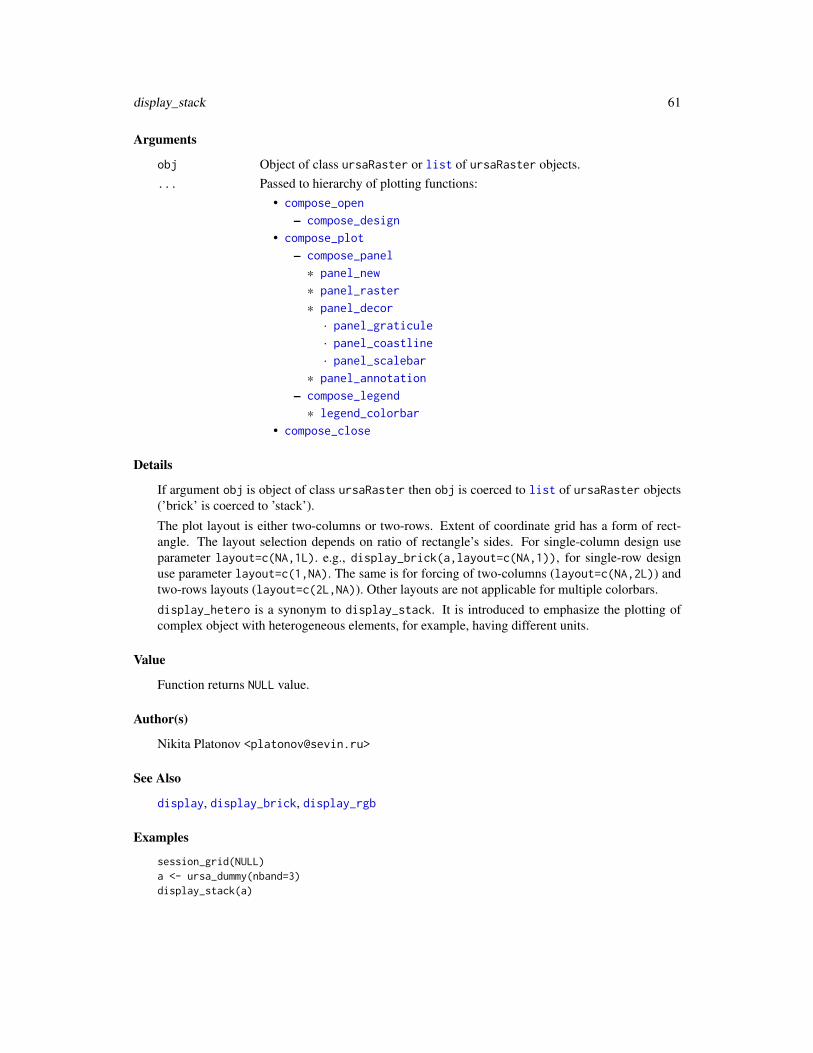
display_stack 61

Arguments

obj Object of class ursaRaster or list of ursaRaster objects.... Passed to hierarchy of plotting functions:

• compose_open

– compose_design

• compose_plot

– compose_panel

* panel_new

* panel_raster

* panel_decor

· panel_graticule

· panel_coastline

· panel_scalebar

* panel_annotation

– compose_legend

* legend_colorbar

• compose_close

Details

If argument obj is object of class ursaRaster then obj is coerced to list of ursaRaster objects(’brick’ is coerced to ’stack’).

The plot layout is either two-columns or two-rows. Extent of coordinate grid has a form of rect-angle. The layout selection depends on ratio of rectangle’s sides. For single-column design useparameter layout=c(NA,1L). e.g., display_brick(a,layout=c(NA,1)), for single-row designuse parameter layout=c(1,NA). The same is for forcing of two-columns (layout=c(NA,2L)) andtwo-rows layouts (layout=c(2L,NA)). Other layouts are not applicable for multiple colorbars.

display_hetero is a synonym to display_stack. It is introduced to emphasize the plotting ofcomplex object with heterogeneous elements, for example, having different units.

Value


Author(s)


See Also

display, display_brick, display_rgb

Examples

session_grid(NULL)a <- ursa_dummy(nband=3)display_stack(a)

62 envi_files

envi_files ENVI File Manipulation

Description

Management of ENVI files similar to functions of OS file manager.

Usage

envi_exists(pattern = ".+", path = ".", all.files = FALSE, full.names = TRUE,recursive = FALSE, ignore.case = TRUE, exact = FALSE)

envi_list(pattern = ".+", path = ".", all.files = FALSE, full.names = recursive,recursive = FALSE, ignore.case = TRUE, exact = FALSE)

envi_remove(pattern = ".+", path = ".", all.files = FALSE, full.names = recursive,recursive = FALSE, ignore.case = TRUE, verbose = FALSE)

envi_copy(src, dst, overwrite = TRUE)envi_rename(src, dst, overwrite = TRUE)

Arguments

pattern Either filename (like basename function) or mask in format of regular expres-sions or full path name.

path Either path name (like dirname function) or ignored if pattern describes fullpath.

all.files A logical value. If FALSE, only the names of visible files are returned. If TRUE,all file names will be returned. Similar to all.files argument in list.filesfunction

full.names A logical value. If TRUE, the directory path is prepended to the file names togive a relative file path. If FALSE, the file names (rather than paths) are returned.Similar to full.names argument in list.files function

recursive Logical. Should the listing recurse into directories? Similar to recursive argu-ment in list.files function

ignore.case Logical. Should pattern-matching be case-insensitive? Similar to ignore.caseargument in list.files function

exact Logical. Attempt to cancel regular expressions.

verbose Logical. TRUE provides some additional information on console.

src Strings of length 1 or more. Name or directory name or path of source ENVIfiles.

dst Strings of length 1 or more. Name or directory name path of destination ENVIfiles. Length is assuming to be equal to length of src

overwrite Logical. TRUE overwrites destinations ENVI files. FALSE does nothing if desti-naton ENVI file exists.

Extract 63

Details

Functions do not view content of any files. The major identifier of ENVI files in file system is ENVIheader (*.hdr) file. Binary file is searching along 1) original *.envi, *.bin, *.img, *.dat extensions,2) externally packing *.gz. *.bz2, *.xz extensions, or 3) packed by this package *.envigz, *.bingzextensions. Functions envi_copy() and envi_rename() keeps original extension of ENVI binaryfile; use file.rename to rename ENVI binary file.

Value

envi_exists() returns integer number of found ENVI files.

envi_list() returns character vector of found ENVI files.

envi_remove() returns character vector of deleted ENVI files.

envi_copy() returns 0L.

envi_rename() returns value of file.rename, which is applied to objects in file system.

Author(s)


Examples

session_grid(NULL)wd <- setwd(tempdir())a1 <- create_envi("tmp1.envi")a2 <- create_envi("tmp2.")close(a1,a2)envi_list()envi_copy("tmp1","tmp3")envi_copy("tmp2","tmp4")envi_list()envi_rename("tmp3","tmp5")envi_list()envi_exists("nofilewithsuchname")envi_exists("tmp[34]")envi_remove(".+")envi_list()setwd(wd)

Extract Extract portion of raster images

Description

This operator is used to get single band or subset of bands from multi-band ursaRaster object.Another purpose is get portions of data including data reading from files.

64 Extract

Usage

## S3 method for class 'ursaRaster'x[i, j, ..., drop = FALSE]

Arguments

x ursaRaster objecti Integer or character. If integer, then band index, specifying bands to extract. If

character, either list of band names or character sting for regular expressionto match band index. In the (spatial, temporal) interpretation of ursaRasterobject j points to temporal component.

j Integer. Line index, specifying lines to extract.... Mentioned for consistence with internal generic function [.

Use regexp=FALSE for matching by match, and regexp=TRUE for matching byPerl-compatible regexps case insensitive grep. Default is FALSE.

drop Not used. For consistence with generic function.

Details

Operator \sQuote{[} is high-level implementation for data reading. If x$value item is not applica-ble, then value of ursaRaster is not in memory. In this case the controlled by i and j portion isread to memory. If both i and j are missing, then x[] reads all values from file.

x[,j] is appropriate for time series analysis and processing in the case bands have relation totemporal observation. Use regrid for geographical subset and cropping.

Value

ursaRaster object with extracter bands. Values ($value item) are in memory.

Warning

It is not allowed to read simultaneously portion of bands and portion of lines from file, e.g.,

x <- open_envi(fname)y <- x[2:3,10:20]close(x)

Such brunch is not implemented in code. You use one of the followed tricks:

x <- open_envi(fname)y <- x[2:3][,20:30]close(x)

or

x <- open_envi(fname)y <- x[,20:30][2:3]close(x)

focal_extrem 65

Author(s)


Examples

session_grid(NULL)## Preparesession_grid(regrid(mul=1/8))a <- pixelsize()w <- c("Monday","Tuesday","Wednesday","Thursday","Friday","Saturday","Sunday"

,"MondayAgain")b <- rep(a/mean(a),length(w))+seq(length(w))-1bandname(b) <- wnr <- ursa_rows(b)bottom <- (as.integer(nr/2)):nrwrite_envi(b,"tmp1",compress=FALSE,interleave="bil")

## Extractprint(b["Monday",regexp=TRUE])print(b["Monday",regexp=FALSE])print(b["s"])print(b["^s"])d1 <- b[6,bottom]rm(b)

## Read from fileb <- open_envi("tmp1")print(b[])print(b[-c(6:8)])d2 <- b[,bottom][6] ## don't use b[6,bottom]close(b)envi_remove("tmp1")

## Compareprint(d1)print(d2)

focal_extrem Extremal spatial filter for image

Description

For each band and for each cell, depending of specification, function finds either minimal or maxi-mal value inside of square window. Focal operation of map algebra.

Usage

focal_extrem(x, kind = c("min", "max"), size = 3, cover = 1e-06,fillNA = FALSE, saveMargin = TRUE, verbose = 0L)

66 focal_extrem

focal_min(x, size = 3, cover = 1e-06, fillNA = FALSE, saveMargin = TRUE, verbose = 0L)focal_max(x, size = 3, cover = 1e-06, fillNA = FALSE, saveMargin = TRUE, verbose = 0L)

Arguments

x Object of class ursaRaster.kind Character. What kind of extremum is required. Allowed values "min" or "max".size Positive numeric. Odd values (3, 5, 7, . . . ) are allowed, but if other value is

specified, then it expanded to the next odd value not less than original value.Default is 3L.

cover Numeric. 0<=cover<=1. Quota for NA values in the focal window in relationto the squared size of the focal window. Quota exceeding leads to recording NAvalue in the cell. Default is cover=1e-6.

fillNA Logical. If TRUE then only NA values of source image can be changed, andnon-NA values of source image are kept without changes. It may provide less re-ducing of spatial resolution in the task of spatial interpolation. Default is FALSE.

saveMargin Logical. If TRUE then adaptive window size is used for cells, where originalwindow goes over image boundary. If FALSE then image is expanded to thehalf size of focal window by NA values and argument cover is applied to thisexpanded part. Default is TRUE.

verbose Integer of 0L, 1L, or 2L, or logical, which is coerced to integer. The level of ver-bosity. Values >0 provide some additional information on console, verbose=1Lis less detailed, verbose=2L is more detailed. Default is 0L.

Details

focal_min(x,...) is a wrapper to focal_extrem(x,"min",...)focal_max(x,...) is a wrapper to focal_extrem(x,"max",...)

Value

Object of class ursaRaster with the same number of bands as in input raster.

Author(s)


See Also

Other focal operations: focal_mean, focal_median.

Examples

session_grid(NULL)a <- ursa_dummy(nband=2,mul=1/8,elements=32)a[a<80] <- NAb.min <- focal_extrem(a,"min",size=4,cover=0.5,verbose=1L)b.max <- focal_extrem(a,"max",size=4,cover=0.5,verbose=1L)print(list(src=a,min=b.min,max=b.max,dif=b.max-b.min))

focal_mean 67

focal_mean Low-pass spatial filter for image.

Description

Low-pass filtering by a square window in the image processing. Focal operation of map algebra.Weight of pixels is proportional to cell area inside of focal window.

Usage

focal_mean(x, size = 3.0, cover = 1e-06, fillNA = FALSE, saveMargin = TRUE,noNA = TRUE, verbose = 0L)

Arguments


size Positive numeric. Size of square focal window. Fractional values are allowed.If size is not odd (3, 5, 7, . . . ), then window size is expanded to the nearest oddvalue not less than original value, and pixels on border are taken with the weight,which is proportional to the cell area inside of original size. Default size=3.

cover Numeric. 0<=cover<=1. Quota for NA values in the focal window in relation toall values. Values are taken with the weight proportional of cell areas inside offocal window. Quota exceeding leads to recording NA value in the cell. Defaultis cover=1e-6.



noNA Logical. If TRUE then NA values are transformed to numerical constant, which isinterpreted as "no data" value. Filter without NA values has more perfomance,and generally filter with pre- and post-transformations of NA values have moreperfomance too. Default is TRUE.


Details

The reference is always central pixel, even if window size is even.

If size=3 then multiplicator is 3^(-2) and elements have equal weights:

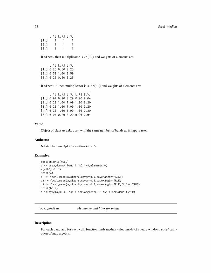
68 focal_median

[,1] [,2] [,3][1,] 1 1 1[2,] 1 1 1[3,] 1 1 1

If size=2 then multiplicator is 2^(-2) and weights of elements are:

[,1] [,2] [,3][1,] 0.25 0.50 0.25[2,] 0.50 1.00 0.50[3,] 0.25 0.50 0.25

If size=3.4 then multiplicator is 3.4^(-2) and weights of elements are:

[,1] [,2] [,3] [,4] [,5][1,] 0.04 0.20 0.20 0.20 0.04[2,] 0.20 1.00 1.00 1.00 0.20[3,] 0.20 1.00 1.00 1.00 0.20[4,] 0.20 1.00 1.00 1.00 0.20[5,] 0.04 0.20 0.20 0.20 0.04

Value


Author(s)


Examples

session_grid(NULL)a <- ursa_dummy(nband=1,mul=1/8,elements=0)a[a<80] <- NAprint(a)b1 <- focal_mean(a,size=6,cover=0.5,saveMargin=FALSE)b2 <- focal_mean(a,size=6,cover=0.5,saveMargin=TRUE)b3 <- focal_mean(a,size=6,cover=0.5,saveMargin=TRUE,fillNA=TRUE)print(b3-a)display(c(a,b1,b2,b3),blank.angle=c(-45,45),blank.density=20)

focal_median Median spatial filter for image

Description

For each band and for each cell, function finds median value inside of square window. Focal oper-ation of map algebra.

focal_median 69

Usage

focal_median(x, size = 3, cover = 1e-06, fillNA = FALSE, saveMargin = TRUE, verbose = 0L)

Arguments


size Positive numeric. Odd values (3, 5, 7, . . . ) are allowed, but if other value isspecified, then it expanded to the next odd value not less than original value.Default is 3L.

cover Numeric. 0<=cover<=1. Quota for NA values in the focal window in relationto the squared size of the focal window. Quota exceeding leads to recording NAvalue in the cell. Default is cover=1e-6.




Value


Author(s)


See Also

Other focal operations: focal_mean, focal_extrem.

Examples

session_grid(NULL)a <- ursa_dummy(1,mul=1/8,elements=0,bandname="src")a[a<80] <- NAbF <- c(fillNA.F=focal_median(a[1],size=5,cover=0.5,fillNA=FALSE))bT <- c(fillNA.T=focal_median(a[1],size=5,cover=0.5,fillNA=TRUE))print(c(diff=bT-bF))d <- c(a,bF,bT)print(d)display(d)

70 focal_special

focal_special Custom spatial filtering for image

Description

For each band and for each cell, function calculates value using specific matrix of square window.Focal operation of map algebra.

Usage

focal_special(x, type = c("custom", "gaussian", "laplacian", "osisaf","hires", "correl", "LoG", "sobel", "sobelG"),

fmask = NULL, size = 3, alpha = 0.5, sigma = (size-1)/4,cover = 1 - 1e-06, fillNA = FALSE, saveMargin = FALSE, verbose = 0L)

Arguments


type Character, which is checked by match.arg.

fmask Numeric square matrix. Filter mask. If NULL then matrix(1,ncol=1) is used.Default is NULL.

size Numeric. Diameter of circuled filter mask. Coerced to the nearest odd value notless than original value.

alpha Nimeric. Parameter alpha for "Laplacian", "LoG", "hires", "correl" filters. Ig-nored for others. Default is 0.5.

sigma Numeric. Parameter sigma for "Gaussian", "LoG" filters. Ignored for others.Default is 0.5.

cover Numeric. 0<=cover<=1. Quota for NA values in the focal window in relationto the squared size of the focal window. Quota exceeding leads to recording NAvalue in the cell. Default is cover=1-1e-6.


saveMargin Logical. If TRUE then adaptive window size is used for cells, where originalwindow goes over image boundary. If FALSE then image is expanded to thehalf size of focal window by NA values and argument cover is applied to thisexpanded part. Default is FALSE.


focal_special 71

Details

Developed under impression from Matlab’s "fspecial".

• type="custom"Filter mask (argument fmask) should be specified manually.

• type="gaussian"Gaussian filter. For cascade filtering (sequence of increasing or decreasing window size)sigma=(size-1)/4 produces the same distribution density relative to window size. If sigmais high but not Inf then it is low-pass filter with diameter=size of circular focal window.

• type="laplacian"Laplacian filter. Only size=3 makes sence. Any size is coerced to size=3.

• type="osisaf"Filter for edge detection. Only size=5 makes sence. Any size is coerced to size=5. TODO(pl): reference

-0.0625 -0.0625 -0.0625 -0.0625 -0.0625-0.0625 0.1250 0.1250 0.1250 -0.0625-0.0625 0.1250 0.0000 0.1250 -0.0625-0.0625 0.1250 0.1250 0.1250 -0.0625-0.0625 -0.0625 -0.0625 -0.0625 -0.0625

• type="hires"Filter for unsharping. Only size=3 makes sence. Any size is coerced to size=3.

-alpha alpha-1 -alphaalpha-1 alpha+5 alpha-1

-alpha alpha-1 -alpha

• type="correl"Filter for contrast increasing. Only size=3 makes sence. Any size is coerced to size=3.

alpha^2 -alpha*(1+alpha^2) alpha^2-alpha*(1+alpha^2) (1+alpha^2)^2 -alpha*(1+alpha^2)

alpha^2 -alpha*(1+alpha^2) alpha^2

• type="LoG"Laplacian of Gaussian. Filter for edge detection. sigma is used, alpha is ignored.

• type="sobel"Two-directional Sobel filtering. Only size=3 makes sence. Any size is coerced to size=3.

• type="sobelG"Sobel gradient. Only size=3 makes sence. Any size is coerced to size=3.

Value


Warning

Laplacian of Gaussian filter (type="LoG") is not implemented clearly due to applying continuous-valued formula to discrete matrix.

72 get_earthdata

Author(s)


References

TODO(pl): at least reference to ’osisaf’.

See Also

Other focal operations: focal_mean, focal_median, focal_extrem.

Examples

session_grid(NULL)v <- round(runif(8,min=-1,max=1),3)customFilter <- matrix(c(v[1:4],-sum(v),v[5:8]),ncol=3)a <- ursa_dummy(1,mul=4/8,elements=32)tpList <- eval(formals("focal_special")$type)res <- c(src=a,as.ursa(bandname=tpList))for (tp in tpList) {

message(tp)res[tp] <- focal_special(a,tp,fmask=customFilter,size=11,sigma=1,alpha=0.8

,saveMargin=0,verbose=2L)}print(res)display(res,decor=FALSE)

get_earthdata Retrive data from Global Imagery Browse Services (GIBS) using APIfor Developers

Description

get_earthdata allows retrieving georeferences optical satellite images of low and moderate spatialresolution (up to 250m per cell) using GIBS API for Developers.

Usage

get_earthdata(bbox = NA, res = c("2km", "1km", "500m", "250m"),date = NA, product = "", geocode = "",expand = 1.05, border = 0, display = FALSE,cache = NA, verbose = FALSE)

get_earthdata 73

Arguments

bbox Numeric of length 4 or character. Spatial extent in the notation c(minx,miny,maxx,maxy).Can be in utits of meters or degrees. If all absolute values are less than 360, thenunits are in degrees and projection is EPSG:3857, else units are in meters andprojection is EPSG:3413. If bbox=NULL, then function return list of availableproducts. If bbox=NA then boundary box is attempted for taking from sessiongrid. If character, then boundary box is taken from geocoding. Default is regionof Vaigach Island.

res Character or numeric. Parameter, which is responsible for dimension of outputraster image. If character, then zoom is selected using keyword list c("2km","1km","500m","250m")for EPSG:3413. If res<10 then it is interpreted as zoom for Web Map Tile Ser-vice (WMTS). If res>100 then res is interpreted as preffered image dimension.If res=NA then res=480L.

date Character or "Date" object. Date for image retrieving. Default is Sys.Date()-1L.

product Character of integer. Data product form GIBS. Currently only MODIS-oriented(corrected reflectance) products are available:

1. "MODIS_Aqua_CorrectedReflectance_Bands721"2. "MODIS_Terra_CorrectedReflectance_Bands721"3. "MODIS_Aqua_CorrectedReflectance_TrueColor"4. "MODIS_Terra_CorrectedReflectance_TrueColor"5. "VIIRS_SNPP_CorrectedReflectance_TrueColor"6. "Coastlines"

Please check actual list by calling get_earthdata(bbox=NULL).If numeric, then index of item among available products. Regular expressionscan be used to simplify value of product, e.g., case-insensitive "aqua 721", "terratruecolor", "suomi", "SNNP".

geocode Character. Keyword for geocode service. Valid values are "google", "nominatim".Default is ""; several services are considered in the case of failure.

expand Numeric. Multiplier for plotting panel zoom in relation to extent of plottinggeometry. Ignored if geocoding is not applied. Default is 1.05.

border Integer. Value in pixels of fixed margins around plotting geometry. Ignored ifgeocoding is not applied. Default is 0L.

display Logical. Value TRUE forces to display image instead of return it. Default isFALSE.

cache Logical. Is cache used? Default is NA, which is interpreted as TRUE for anyrequested date excepting not late time of today (approximately 17:00 UTC).

verbose Logical. Value TRUE may provide some additional information on console. De-fault is FALSE.

Details

Argument method="libcurl" is used in function download.file for tile downloading. Pleasecheck capabilities("libcurl").

Valid zoom values (e. g., specified via res argument) are 3:6 for EPSG:3413 and 0:8 for EPSG:3587.

74 glance

Longitude 180 degrees has a seam in EPSG:3857 (e.g., see bbox=c(170,68,-170,73) and bbox=c(-1600000,1308000,-1370000,1570000)for Wrangel Island. If region crosses longitude 180 degrees in EPSG:3857, then the prior day istaken for Western Hemisphere.

Value

If bbox=NULL, then character vector of available products.

If display=FALSE then object of class ursaRaster with RGBA image.

If display=TRUE then returned value of display_brick.

Author(s)


References

GIBS API for Developers

Examples

session_grid(NULL)pr <- get_earthdata()print(pr,quote=FALSE)

## internet connection is required -- begina1 <- get_earthdata(bbox=c(2000000,400000,2300000,700000))display(a1)

## internet connection is required -- enda2 <- get_earthdata(product=2,date=Sys.Date()-7L,res=7,bbox=c(57.8,69.4,62.3,70.8))display(a2)

glance Command line utility for spatial view of raster or vector GIS file.

Description

glance is a parser of command line arguments for non-public function .glance, which createsmulti-panel plots for each attribute of vector file or for each band of raster file.

Usage

glance(...)

# non-public.glance(dsn, layer = ".*", grid = NULL, field = ".+", size = NA, expand = 1,

border = 27, lat0 = NA, lon0 = NA, resetProj = FALSE, resetGrid = FALSE,

https://wiki.earthdata.nasa.gov/display/GIBS/GIBS+API+for+Developers

glance 75

style = "auto", feature = c("auto", "field", "geometry"), alpha = NA,basemap.order = c("after", "before"), basemap.alpha = NA,engine = c("native", "sp", "sf"), geocode = "", place="",

area = c("bounding", "point", "shape"), zoom = NA, gdal_rasterize = FALSE,silent = FALSE, verbose = FALSE, ...)

Arguments

dsn Character or object of either ursaRaster, Spatial, or sf classes. If character,then data source name (interpretation varies by driver - for some drivers, dsn isa file name, but may also be a folder, or contain the name and access credentialsof a database).

layer Character or integer. If integer, then layer index. If character, then pattern (regu-lar expressions) to recognize layer by name. Only one layer selection is allowed.If selected more then one layer, the error message contains indices and names oflayers. Usually, datasets (e. g., "ESRI Shapefile") have only one layer. Defaultis ".*"; interpreted as all layers.

grid Object of class ursaGrid or NULL. Reference CRS and boundary box for visu-alization. If NULL, then CRS and boundary box are zoomed to layer. Default isNULL.

field Character. Pattern for field (attribute, column,...) selection by name using regu-lar expressions. Multiple selection is allowed. Default is ".+"; all fields.

size Integer of length 1 or 2 or character of length 1. Size of plotting panel in pixels.If character, then parsed to integer of length 1 or 2. Length 2 is used only for webcartography. If length 1, then size defines width of panel, and height is definedautomatically. If integer, then width of panel for plotting in pixels. Default isNA; for web cartogrpaphy value of maximal size of static maps, and code640 forother cases.

expand Numeric. Multiplier for plotting panel zoom in relation to extent of plottinggeometry. Default is 1.0.

border Integer. Value in pixels of fixed margins around plotting geometry. Default is27L.

lat0 Numeric. Parallel os zero distortion. If NA, then parallel os zero distortion is de-termined from object geometry. Actual for "+proj=stere" projections. Defaultis NA.

lon0 Numeric. Central meridian, which have vertical direction on the plot. If NA, thencentral meridian is determined from object geometry. Default is NA.

resetProj Logical. Value TRUE overwrites projection of vector file. Default is FALSE.

resetGrid Logical. If TRUE, then session grid is ignored, and new session grid is assignedfrom input file. If FALSE, then input file is nested in the session grid.

style Character. Either projection class or source of web-catrogrpaphy for basemap.Specified by a sentence of words separated by spaces.

76 glance

• Projection classValid values are "stere", "laea", "merc", "longlat". Default is key-word "auto"; use object projection, if this projection differs from projec-tion class "+longlat", otherwise, projection ("stere" or "merc") is deter-mined internally.

• Web cartography.– Static map

Valid values are "google", "openstreetmap", "sputnikmap". Staticmaps have priority over tile services. however additional word "static"can be specified in the sentence, e.g., "openstreetmap static" or"static google". Additional parameters for request to web-script canbe added in the sentence in the form "argument1=value1 [argument2=value2]",e.g., style="google static maptype=terrain language=ru-RU scale=2".

– Tile serviceSupported tile services can be returned by calling of non-public func-tion ursa:::.tileService() without arguments. Valid values are"mapnik", "cycle", "transport", "mapsurfer", "sputnik", "thunderforest","carto", "kosmosnimki", etc.

By default, if data has no data fields (e. g., geometry only), then basemapis drawn in color, else in grayscale. Adding word "color" (or "colour")to the sentence forces to use colored basemap. Adding word "gray" (or"grey", "greyscale", "grayscale") to the sentence forces to use coloredbasemap.The order of words in the sentence is any.

Keywords "google", "openstreetmap" force to use "Google Static Map" or"OpenStreetMap static map images" for basemap; the resulted projection hasclass "+proj=merc".

feature Character. Appearance of visualization. If "field" then data of each field isplotted on separate panel (number of panels is equal to number of columns inattribute table). If "geometry" then each feature is plotted on separate panel(number of panels is equal to number of rows in attribute table). Default is"auto"; if intersects of features are found, then "geometry" is used, else "field".

basemap.order Character. The order of basemap layer rendering in the case of web-cartographybasemap.If "before", then basemap is plotted before object plot. If "after",then basemap is plotted over object.

basemap.alpha Character. The saturation of basemap in the case of web-cartography basemap.Default is NA; basemap.alpha=0.5 for basemap.order="before" and basemap.alpha=0.35for basemap.order="after".

alpha Character. The opacity of plotted object. Default is NA; 0.75 for basemap.order="before"in web-cartogrpaphy style, 1.00 - in all other cases.

engine Character keyword. Forcing to vector files processing by functions from pack-age sp (engine="sp") or package sf (engine="sf", if sf is installed). Defaultis "native"; if dsn is Spatial object or if sf is not installed, then "sp" is used.

geocode Character. Keyword for geocode service. Valid values are "google", "nominatim".If dsn is character and file dsn not found, then trying to interpret dsn as a re-quest to geocode service. The output is only basemap of web cartogrpaphy.

glance 77

Default is ""; several services are considered in the case of failure. Is styleis not specified, then "Google Static Map" is used for geocode="google", and"OpenStreetMap static map images" for geocode="nominatim".

place Character. Type of geographical object (river, island) in the geocoding request.If geocode service is "nominatim", then place is searched among attributes"class" and "type". Default is ""; any object is acceptable.

area Character. Keyword of spatial class of geocoded object. "bounding" is usedfor boundary box; "point" is used for point. Default value is extracted bymatch.arg(area).

zoom Positive integer or character. Zooming if web-cartography is applied for basemap.If integer, then value of zoom for tile services and staticmap. If character, then"0" means zoom by default (defined internally), "+1" means increment on 1 ofdefault zoom, "+2" means zoom increment on 2, "-1" means zoom decrementon 1, "-2" means zoom decrement on 2, etc. Default is NA; zoom is definedinternally.

gdal_rasterize Logical. If TRUE and GDAL utilities are in the system search path, then overlayfor panels is formed via rastetization of vector file. GDAL utility "gdal_rasterize"is used. Note, that GDAL (system level) is optional for this package. Default isFALSE.

silent Logical. Value TRUE cancels progress bar. Default is FALSE.

verbose Logical. Logical. Value TRUE may provide some additional information onconsole. Default is FALSE.

... glance: Arguments, which are passed to .glance or to display..glance: Arguments, which are passed to static maps API, colorize, display,etc.

Details

Command line usage implies set of arguments using pair: argument name and argument value.and values in the format "[name1=]value1 [name2]=value2". No spaces around = (equal symbol).Argument name can be omitted, symbol = is omitted too. If argument value has spaces, then argu-ment value should be surrounded by double quotes (fname="my test.shp"). If argument value ismatched to R function, then such value should be surrounded by single quotes (layer='density').

Command line usage example: Rscript -e ursa::glance() 'final_more_than_032.sqlite'attr="select" resetProj=TRUE expand=1.5

For OS Windows, bat-file can be created for raster and vector file association: Rscript -e ursa::glance()%*

Command line usage implies external software for PNG view session_pngviewer(TRUE).

Value

glance returns integer: 0L - successful, 10L - call without arguments.

Note

Package sf is ’Suggested’ for package ursa.

78 global operator

Author(s)


Examples

session_grid(NULL)f <- system.file("vectors","scot_BNG.shp",package="rgdal")glance(f,style="merc",field="(NAME|COUNT)")cmd <- paste("Rscript --vanilla -e ursa::glance()",paste0("\"",f,"\"")

,"style=\"merc\"","field=\"(lon|lat)\"")cat(" --------- Try in command line: -----------\n")message(cmd)cat(" ----------- end of quoting ---------------\n")## windows: figure will be opened using *.png file association

try(system(cmd,wait=FALSE))

require(sp)a <- data.frame(lat=c(70.734,71.657),lon=c(178.577,-177.38),place="Wrangel Island")coordinates(a) <- ~lon+latproj4string(a) <- "+init=epsg:4326"

## internet connection is requiredglance(a,style="google color maptype=terrain")

## internet connection is requiredglance(a,style="openstreetmap color")

## internet connection is requiredglance(a,style="mapnik color tile")

## internet connection is requiredglance("Svalbard")

global operator Extract certains statistics for whole image

Description

Function from this global.\emph{FUN} list returns required statistics FUN for the whole image.

Usage

global_mean(x, ursa = FALSE, ...)global_median(x, ursa = FALSE, ...)global_sd(x, ursa = FALSE, ...)global_sum(x, ursa = FALSE, ...)global_min(x, ursa = FALSE, ...)

global operator 79

global_max(x, ursa = FALSE, ...)global_n(x, ursa = FALSE, ...)global_nNA(x, ursa = FALSE, ...)global_range(x, ursa = FALSE, ...)

Arguments


ursa Logical. The class of returned value. If FALSE then numeric vector of lengthone is returned (for global_range vector has length two). If TRUE then returnedvalue is single-band raster image (two-bands image for global_range) withconstant value for all cells (blank image). Default is FALSE.

... Arguments in function global.\emph{FUN} which are passed to function \emph{FUN}.

Details

For any function global.\emph{FUN}, if argument na.rm is not in ..., then \emph{FUN} is calledwith forced na.rm=TRUE.global_range\emph{list of arguments} is implemented as c(global_min(\emph{list of arguments}), global_max(\emph{list of ar-guments})) with the same list of arguments.

Alternative method to get global statistics is function applying directly to the raster value. For exam-ple, sd(ursa_value(x,na.rm=TRUE)). This way is also appropriate for missing global functions:for example, var(ursa_value(x,na.rm=TRUE)).

Value

If ursa=FALSE then numeric.If ursa=TRUE then object of class ursaRaster.

Author(s)


Examples

session_grid(NULL)a <- ursa_dummy(2,min=-40,max=80)a[a<0] <- NAprint(a)a.mean <- global_mean(a)a.sd <- global_sd(a)a.sum <- global_sum(a)a.min <- global_min(a)a.max <- global_max(a)a.median <- global_median(a)print(c(mean=a.mean,sd=a.sd,sum=a.sum,min=a.min,max=a.max,median=a.median))v.max <- max(ursa_value(a),na.rm=TRUE)print(c('global_max()'=a.max,'max(ursa_value())'=v.max,dif=a.max-v.max))r.max <- global_max(a,ursa=TRUE)print(r.max)

80 groupGeneric

b <- c(a,'appended scalar value'=a.max)print(b)

groupGeneric Group Generic Functions for raster image

Description

These functions implement arithmetical and logical operations, mathematical functions for objectsof class ursaRaster as well as group generic functions from package base do similar for S3 class.These are local operations in the raster algebra (map algebra).

Usage

## S3 method for class 'ursaRaster'Ops(e1, e2 = NULL)

## S3 method for class 'ursaRaster'Math(x, ...)

## S3 method for class 'ursaRaster'Complex(z)

## S3 method for class 'ursaRaster'Summary(..., na.rm = FALSE)

Arguments

x ursaRaster object

e1 ursaRaster object

e2 Numeric of length 1, matrix, array, or ursaRaster object.

na.rm Logical. If na.rm=TRUE then no-data values are omitted.

z Any.

... For group Math - further arguments passed to methods. See description forgeneric.For group Summary - set of arguments, which are recognized via their names(using regular expressions), position and classes.

.* Position 1. Object of class ursaRaster.cov|cvr Position >1. Numeric between 0 and 1. If proportion of bands with

no data for given location exceeds cover then output value is NA (no data).Default is 0.5-1e-3.

w Position >1. Numeric of length number of bands or NULL. Band weights forweighted mean. Default is NULL; all bands have equal weights.

groupGeneric 81

name Position >1. Character of length 1. Band name for output raster. Defaultis ""; band name is assigned automatically.

verb(ose)* Position >1. Logical. verbose=TRUE provides some additionalinformation on console. Default is FALSE.

Details

The groups are 'Summary', 'Ops', 'Math', and 'Complex’. See “Details” section in the S3 GenericFunctions help page.

The group 'Complex' is unsupported.

The groups 'Math' and 'Summary' are implemented completely.

The group 'Ops' has some features.

• Logical operators "<", ">", "<=", ">=", "==", \"!=" return 'NA' for value FALSE and '1' forvalue TRUE to organize cells’ masking.

• Unary operator "!" is equal to binary operator operators "!=", where the second argument isscalar value 0 (zero).

The operators of groups 'Math' and 'Ops' destroy color tables.

For group 'Summary' the realization of local operators of map algebra is possible via apply func-tion:apply(ursa_value(obj),1,function(x) {y <-sd(x)+1;y})oras.ursa(apply(obj,1:2,function(x) {y <-sd(x)+1;y}))

Value

Operators of groups 'Complex' return stopOperators of groups 'Math', 'Ops', 'Summary' return object of class ursaRaster

Author(s)


See Also

Other S3 generic function for local operations of map algebra are mean, median.Standard deviation (local) and certain local operations can be extracted using local_stat.

Examples

session_grid(NULL)session_grid(regrid(mul=1/4))a1 <- ursa_dummy(nband=3,min=-5*pi,max=5*pi)print(a1)

try(print(complex1 <- Re(a1)))

print(math1 <- a2 <- round(a1))

82 head

print(math1 <- sin(a1))print(math2 <- floor(a1))print(math3 <- ceiling(a1))print(math4 <- cumsum(a1)) ## does this have a sense for rasters?

print(ops1 <- a1-2*rev(a1)+mean(a1))print(mean(ops1)) ## vanishinga2 <- ursa_new(value=c(1,2,4),bandname=c("single","double","quadruple"))print(a2)print(ops2 <- a2[1]==a2[2])print(ops3 <- a2[1]==a2[2]/2)print(ops4 <- a1>0)print(a1[a1>0])

print(sum1 <- sum(a1))print(sum2 <- range(a1))

head Extract first and last bands of raster image

Description

Functions to extract first bands (head), last bands (tail) and first+last bands (series) of rasterimage.

Usage

## S3 method for class 'ursaRaster'head(x, n = 3L, ...)

## S3 method for class 'ursaRaster'tail(x, n = 3L, ...)

series(x, n = 3L, s=170, ...)

Arguments


n Positive integer. Number of extracted bands.

s Positive numeric. Maximal size of memory in MB for extracted raster image inthe assumption that class of values is numeric.

... Not used.

Details

Function series combines consequtive calling head(x); tail(x) with checking the size of ex-tracted part of raster image. If size exceeds specified value of the argument s, then number ofextracted bands n is decreased.

hist 83

Value


Author(s)


Examples

session_grid(NULL)session_grid(regrid(mul=1/8))a <- ursa_dummy(nband=101)print(head(a))print(tail(a))print(series(a,2))print(series(a[1:5]))

hist Histogram of raster image

Description

Two functions for manipulation with histograms. In function hist values of ursaRaster objectsare passed to generic function hist, which allows compute and optionally plot histograms. Otherfunction, histogram, plots histogram in the graphical device png directly.

Usage

## S3 method for class 'ursaRaster'hist(x, ...)

ursa_hist(obj, width = 800, height = 600, ...)histogram(...)

Arguments

obj, x Object of class ursaRaster

width Positive integer. Width of histogram’s panel.

height Positive integer. Height of histogram’s panel.

... Other arguments, which are passed to colorize and compose_open functions.

84 identify

Details

histogram is synonym of ursa_hist.

Function hist for ursaRaster object is defined as hist(ursa_value(obj),...).In the function histogram each bin corresponds to category. The image splitting to categoriesis realized via colorize function. The panel of plotting is constucted using artificial coordinatesystem without geographical projection. The purpose of compose_open function is prepare layoutfor plotting raster images; in the case of histogram, the purpose of this function is prepare layoutfor plotting histogram

Value

Function histogram returns 0L.

Author(s)


See Also

colorize is used to define histogram bins.compose_open prepares panel for histogram plotting.hist computes and plots histograms.

Examples

session_grid(NULL)a <- pixelsize()hist(a)histogram(a,breaks=21)

identify Get value and coordinates from location

Description

Functions to extract values of raster image from given location, specified by coordinates in rasterprojection, by cell position or by geogpaphical coordinates. Additional utils to convert cell positionand planar coordinates mutually.

Usage

value_xy(obj, ...)

value_ll(obj, ...)

value_cr(obj, ...)

identify 85

coord_xy(obj, ...)

coord_cr(obj, ...)

Arguments


... the set of arguments, which are recognized via their names (using regular ex-pressions) and classes:

Matched pattern Function Used nameind *_* ind Index (positive integer) in internal value storage.^c *_cr col Integer of non-zero length. Index of column/sample Length of column and row indices should be the same for creating set of two-dimension coordinates.

^r *_cr row Integer of non-zero length. Index of row/line. Length of column and row indices should be the same for creating set of two-dimension coordinates.^x *_xy x Numeric of non-zero length. X-axis coordinate in grid of obj. The length of X-axis and Y-axis coordinates should be the same for creating set of two-dimension coordinates.^y *_xy y Numeric of non-zero length. Y-axis coordinate in grid of obj. The length of X-axis and Y-axis coordinates should be the same for creating set of two-dimension coordinates.^lon value_ll lon Longitude. The length of longitudes and latitudes should be the same for creating set of two-dimension coordinates.^lat value_ll lat Latitude. The length of longitudes and latitudes should be the same for creating set of two-dimension coordinates.

Details

value_xy returns values for location, which is specified by planar coordinates (x, y).value_cr returns values for location, which is specified by cell posisition (column, row) relative toupper-left corner of image .value_ll returns values for location, which is specified by longitude and latitude (long, lat).

coord_xy transforms planar coordinates (x, y) to cell position (column, row).coord_cr transforms cell position (column, row) to planar coordinates (x, y).

It is required to use a couple of coordinate vectors: (x,y), (c,r) or (lon,lat) of the same length.The unary argument is interpreted as index in internal value storage.

Position in column/row coordinates starts from upper-lever corner. The cell of upper-level cornerhas (1, 1) coordinates (in R indices starts from 1L), whereas in some GIS the same corner cell has(0, 0) coordinates.

The column names of returned matrix are character format of index in internal value storage. Thisindex can be specify in any function as argument ind instead of coordinates (planar, geographical,cell position).

Value

For value.* numeric matrix of raster values. Band values for specific coordinates are by column.Set of specific coordinates are by row. rownames are band names, and colnames are index ininternal value storage.

For coord.* numeric matrix of coordinates with a vector of couple coordinates, one coordinate perone row. rownames are returned coordinates, and colnames are index in internal value storage.

86 ignorevalue

Author(s)


Examples

session_grid(NULL)set.seed(352)a <- as.integer(ursa_dummy(3,min=0,max=999))ind <- which(ursa_value(a[1])==890)print(ind)msk <- a[1]==890am <- a[msk]b <- as.data.frame(am)b$jx <- b$x+runif(nrow(b),min=-1000,max=1000)b$jy <- b$y+runif(nrow(b),min=-1000,max=1000)print(b)cr1 <- coord_xy(a,x=b$jx,y=b$jy)cr2 <- coord_xy(a,y=b$y,x=b$x)cr3 <- coord_xy(a,ind=ind)print(cr1)print(all.equal(cr1,cr2,cr3))xy1 <- coord_cr(a,c=cr1["c",],r=cr1["r",])print(xy1)print(c(identical(unname(xy1["x",]),b[,"x",drop=TRUE])

,identical(unname(xy1["y",]),b[,"y",drop=TRUE])))val1 <- value_xy(a,x=b$jx,y=b$jy)val2 <- value_xy(a,x=b$x,y=b$y)val3 <- value_cr(a,ind=ind)val4 <- value_cr(a,c=cr1["c",],r=cr1["r",])print(val1)print(all.equal(val1,val2,val3,val4))ps <- pixelsize()ll <- c(lon=180,lat=70)v <- value_ll(ps,lon=180,lat=70)print(c('True scale'=v/with(ursa_grid(ps),1e-6*resx*resy)))

ignorevalue Extract and assign ‘nodata’ value of raster images.

Description

Ignored values (aka ’nodata’) are implemented via NA values, and are optional for raster imagesin memory. However, to avoid ambiguity for data storage, it is desirable to specify ignored value.“ENVI .hdr Labelled Raster” supports ‘nodata’ by means of “data ignore value” field in the headerfile.

ignorevalue 87

Usage

ignorevalue(obj)ursa_nodata(obj)

ignorevalue(obj) <- valueursa_nodata(obj) <- value

Arguments

obj ursaRaster object.

value Integer of numeric of length one. Ignored (‘nodata’) value.

Details

ursa_nodata is synonym to ignorevalue for both Extract and Replace methods.

The ‘nodata’ value of raster image obj is specified in the item obj$con$nodata.

If values of raster image are in memory then replace function ignorevalue<- also changes ‘nodata’values to NA values.

Value

Extract function ignorevalue returns value of $con$nodata item of ursaRaster object.

Replace function ignorevalue<- returns ursaRaster with modified $con$nodata item.

Author(s)


Examples

session_grid(NULL)a <- round(ursa_dummy(nband=1,min=0.500001,max=4.499999))print(a)print(as.table(a))print(ignorevalue(a))ignorevalue(a) <- NAprint(as.table(a))print(ignorevalue(a))ignorevalue(a) <- 4print(as.table(a))print(ignorevalue(a))print(a)

88 is.na

is.na ‘No data’ values for raster images.

Description

The "Extract" function is.na creates mask for each band. In this mask value 1L corresponds to NAvalue in the source image, and value NA corresponds non-missing values in the source image. The"Replacement" function is.na<- assigns numerical value for cells with ‘no data’ value.

Usage

## S3 method for class 'ursaRaster'is.na(x)

## S3 method for class 'ursaRaster'is.infinite(x)

## S3 method for class 'ursaRaster'is.nan(x)

## S3 replacement method for class 'ursaRaster'is.na(x) <- value

Arguments


value Numeric.

Details

These functions are corresponded to local operators of map algebra.

Value

"Extract" functions is.na, is.infinite, is.nan return object of class ursaRaster.

"Replacement" function is.na<- modifies object of class ursaRaster.

Author(s)


Examples

session_grid(NULL)session_grid(regrid(mul=1/4))a <- ursa_dummy(nband=2,min=0,max=100)print(a)

legend_align 89

print(is.na(a))a2 <- ursa_new(nband=2)print(a2)print(is.na(a2))a3 <- aa3[a3<30 | a3>70] <- NAprint(a3)print(is.na(a3))is.na(a3) <- 200print(a3)

legend_align Align caption position for legend

Description

When multiple panels on the same axis, the different order of values or different units of valuesmay provoke different shifting of values and caption from panels. legend_align repairs it bythe taking names of classes of the required rasters. The function output is for argument aling oflegend_colorbar.

Usage

legend_align(obj)

Arguments

obj Object of class ursaColorTable, or object of class ursaRaster, or list ofursaColorTable or ursaRaster objects.

Details

The function is defined as:

c(unlist(sapply(obj,function(x) names(ursa_colortable(x)))))

Value

Character vector.

Author(s)


See Also

legend_colorbar

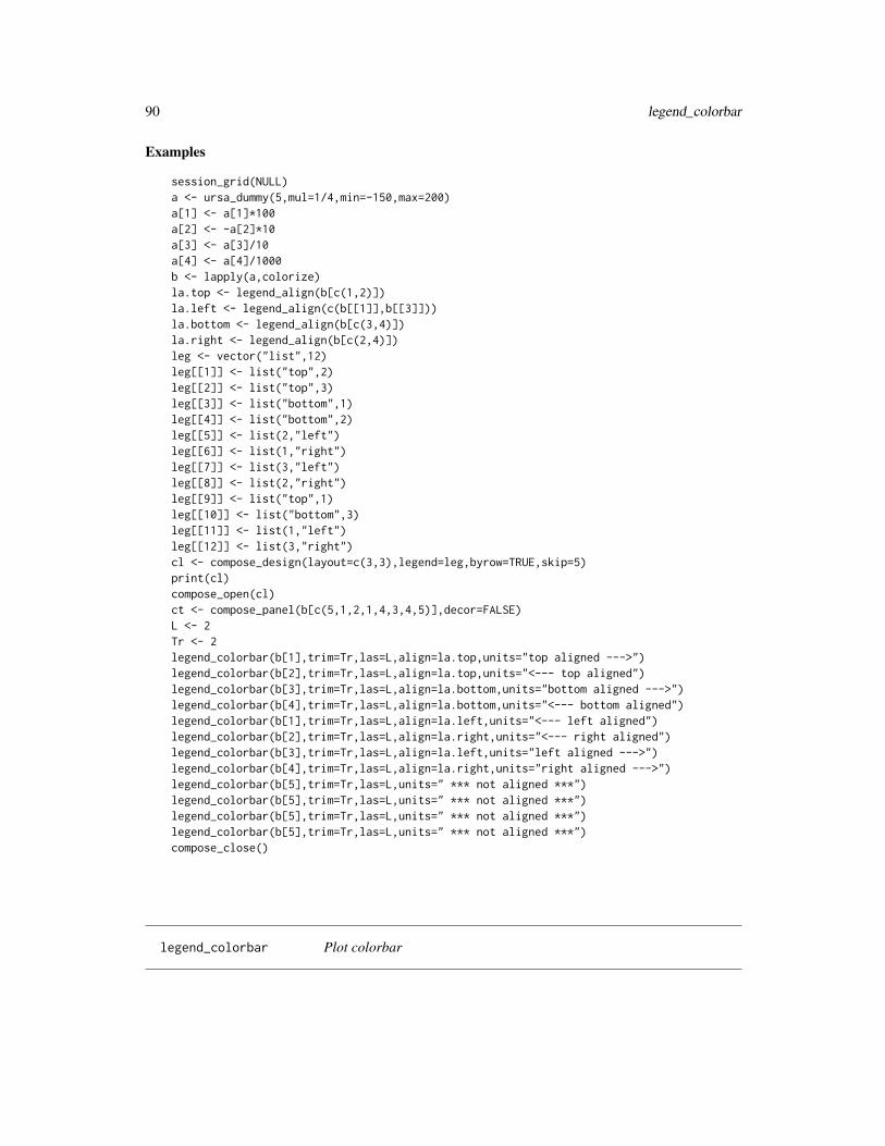
90 legend_colorbar

Examples

session_grid(NULL)a <- ursa_dummy(5,mul=1/4,min=-150,max=200)a[1] <- a[1]*100a[2] <- -a[2]*10a[3] <- a[3]/10a[4] <- a[4]/1000b <- lapply(a,colorize)la.top <- legend_align(b[c(1,2)])la.left <- legend_align(c(b[[1]],b[[3]]))la.bottom <- legend_align(b[c(3,4)])la.right <- legend_align(b[c(2,4)])leg <- vector("list",12)leg[[1]] <- list("top",2)leg[[2]] <- list("top",3)leg[[3]] <- list("bottom",1)leg[[4]] <- list("bottom",2)leg[[5]] <- list(2,"left")leg[[6]] <- list(1,"right")leg[[7]] <- list(3,"left")leg[[8]] <- list(2,"right")leg[[9]] <- list("top",1)leg[[10]] <- list("bottom",3)leg[[11]] <- list(1,"left")leg[[12]] <- list(3,"right")cl <- compose_design(layout=c(3,3),legend=leg,byrow=TRUE,skip=5)print(cl)compose_open(cl)ct <- compose_panel(b[c(5,1,2,1,4,3,4,5)],decor=FALSE)L <- 2Tr <- 2legend_colorbar(b[1],trim=Tr,las=L,align=la.top,units="top aligned --->")legend_colorbar(b[2],trim=Tr,las=L,align=la.top,units="<--- top aligned")legend_colorbar(b[3],trim=Tr,las=L,align=la.bottom,units="bottom aligned --->")legend_colorbar(b[4],trim=Tr,las=L,align=la.bottom,units="<--- bottom aligned")legend_colorbar(b[1],trim=Tr,las=L,align=la.left,units="<--- left aligned")legend_colorbar(b[2],trim=Tr,las=L,align=la.right,units="<--- right aligned")legend_colorbar(b[3],trim=Tr,las=L,align=la.left,units="left aligned --->")legend_colorbar(b[4],trim=Tr,las=L,align=la.right,units="right aligned --->")legend_colorbar(b[5],trim=Tr,las=L,units=" *** not aligned ***")legend_colorbar(b[5],trim=Tr,las=L,units=" *** not aligned ***")legend_colorbar(b[5],trim=Tr,las=L,units=" *** not aligned ***")legend_colorbar(b[5],trim=Tr,las=L,units=" *** not aligned ***")compose_close()

legend_colorbar Plot colorbar

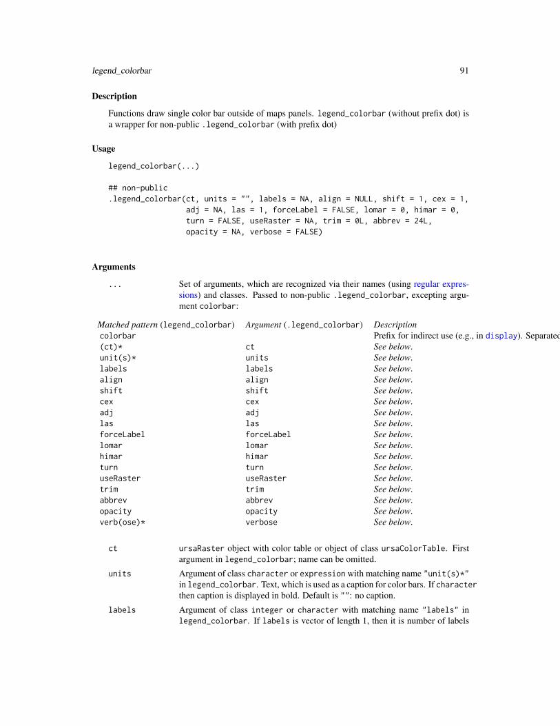
legend_colorbar 91

Description

Functions draw single color bar outside of maps panels. legend_colorbar (without prefix dot) isa wrapper for non-public .legend_colorbar (with prefix dot)

Usage

legend_colorbar(...)

## non-public.legend_colorbar(ct, units = "", labels = NA, align = NULL, shift = 1, cex = 1,

adj = NA, las = 1, forceLabel = FALSE, lomar = 0, himar = 0,turn = FALSE, useRaster = NA, trim = 0L, abbrev = 24L,opacity = NA, verbose = FALSE)

Arguments

... Set of arguments, which are recognized via their names (using regular expres-sions) and classes. Passed to non-public .legend_colorbar, excepting argu-ment colorbar:

Matched pattern (legend_colorbar) Argument (.legend_colorbar) Descriptioncolorbar Prefix for indirect use (e.g., in display). Separated by a dot ".", e.g., colorbar.units="mbar".(ct)* ct See below.unit(s)* units See below.labels labels See below.align align See below.shift shift See below.cex cex See below.adj adj See below.las las See below.forceLabel forceLabel See below.lomar lomar See below.himar himar See below.turn turn See below.useRaster useRaster See below.trim trim See below.abbrev abbrev See below.opacity opacity See below.verb(ose)* verbose See below.

ct ursaRaster object with color table or object of class ursaColorTable. Firstargument in legend_colorbar; name can be omitted.

units Argument of class character or expression with matching name "unit(s)*"in legend_colorbar. Text, which is used as a caption for color bars. If characterthen caption is displayed in bold. Default is "": no caption.

labels Argument of class integer or character with matching name "labels" inlegend_colorbar. If labels is vector of length 1, then it is number of labels

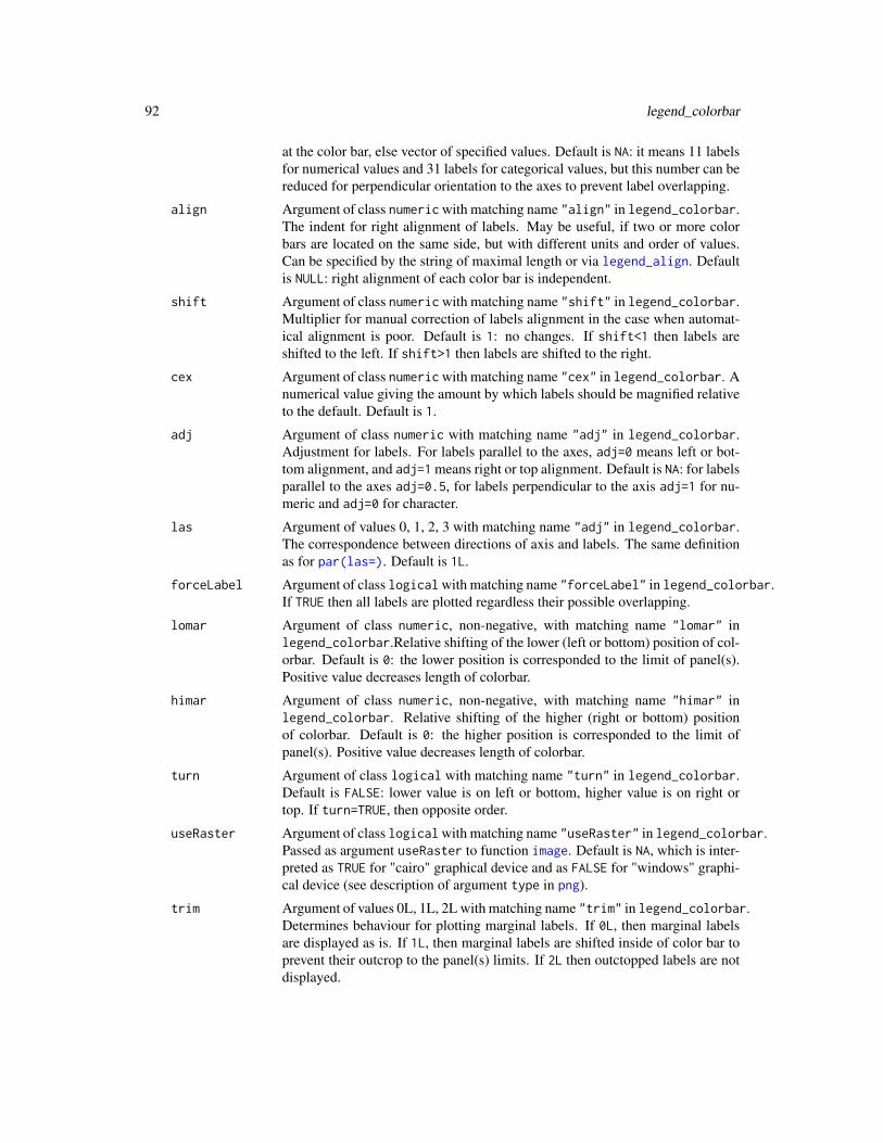
92 legend_colorbar

at the color bar, else vector of specified values. Default is NA: it means 11 labelsfor numerical values and 31 labels for categorical values, but this number can bereduced for perpendicular orientation to the axes to prevent label overlapping.

align Argument of class numeric with matching name "align" in legend_colorbar.The indent for right alignment of labels. May be useful, if two or more colorbars are located on the same side, but with different units and order of values.Can be specified by the string of maximal length or via legend_align. Defaultis NULL: right alignment of each color bar is independent.

shift Argument of class numeric with matching name "shift" in legend_colorbar.Multiplier for manual correction of labels alignment in the case when automat-ical alignment is poor. Default is 1: no changes. If shift<1 then labels areshifted to the left. If shift>1 then labels are shifted to the right.

cex Argument of class numeric with matching name "cex" in legend_colorbar. Anumerical value giving the amount by which labels should be magnified relativeto the default. Default is 1.

adj Argument of class numeric with matching name "adj" in legend_colorbar.Adjustment for labels. For labels parallel to the axes, adj=0 means left or bot-tom alignment, and adj=1 means right or top alignment. Default is NA: for labelsparallel to the axes adj=0.5, for labels perpendicular to the axis adj=1 for nu-meric and adj=0 for character.

las Argument of values 0, 1, 2, 3 with matching name "adj" in legend_colorbar.The correspondence between directions of axis and labels. The same definitionas for par(las=). Default is 1L.

forceLabel Argument of class logical with matching name "forceLabel" in legend_colorbar.If TRUE then all labels are plotted regardless their possible overlapping.

lomar Argument of class numeric, non-negative, with matching name "lomar" inlegend_colorbar.Relative shifting of the lower (left or bottom) position of col-orbar. Default is 0: the lower position is corresponded to the limit of panel(s).Positive value decreases length of colorbar.

himar Argument of class numeric, non-negative, with matching name "himar" inlegend_colorbar. Relative shifting of the higher (right or bottom) positionof colorbar. Default is 0: the higher position is corresponded to the limit ofpanel(s). Positive value decreases length of colorbar.

turn Argument of class logical with matching name "turn" in legend_colorbar.Default is FALSE: lower value is on left or bottom, higher value is on right ortop. If turn=TRUE, then opposite order.

useRaster Argument of class logical with matching name "useRaster" in legend_colorbar.Passed as argument useRaster to function image. Default is NA, which is inter-preted as TRUE for "cairo" graphical device and as FALSE for "windows" graphi-cal device (see description of argument type in png).

trim Argument of values 0L, 1L, 2L with matching name "trim" in legend_colorbar.Determines behaviour for plotting marginal labels. If 0L, then marginal labelsare displayed as is. If 1L, then marginal labels are shifted inside of color bar toprevent their outcrop to the panel(s) limits. If 2L then outctopped labels are notdisplayed.

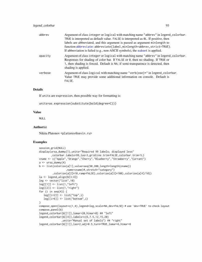
legend_colorbar 93

abbrev Argument of class integer or logical with matching name "abbrev" in legend_colorbar.TRUE is interpreted as default value. FALSE is interpreted as 0L. If positive, thenlabels are abbreviated, and this argument is passed as argument minlength tofunction abbreviate: abbreviate(label,minlength=abbrev,strict=TRUE).If abbreviation is failed (e.g., non-ASCII symbols), the subset is applied.

opacity Argument of class integer or logical with matching name "abbrev" in legend_colorbar.Responses for shading of color bar. If FALSE or 0, then no shading. If TRUE or1, then shading is forced. Default is NA; if semi-transparence is detected, thenshading is applied.

verbose Argument of class logical with matching name "verb(ose)*" in legend_colorbar.Value TRUE may provide some additional information on console. Default isFALSE.

Details

If units are expression, then possible way for formatting is:

units=as.expression(substitute(bold(degree*C)))

Value

NULL

Author(s)


Examples

session_grid(NULL)display(ursa_dummy(1),units="Required 99 labels; displayed less"

,colorbar.labels=99,las=3,gridline.trim=FALSE,colorbar.trim=1L)cname <- c("Apple","Orange","Cherry","Blueberry","Strawberry","Currant")a <- ursa_dummy(4)b <- list(colorize(a[1],value=seq(50,200,length=length(cname))

,name=cname)#,stretch="category"),colorize(a[2]*10,ramp=FALSE),colorize(a[3]*100),colorize(a[4]/10))

la <- legend_align(b[3:4])leg <- vector("list",10)leg[[1]] <- list(1,"left")leg[[2]] <- list(1,"right")for (i in seq(4)) {

leg[[i+2]] <- list("top",i)leg[[i+6]] <- list("bottom",i)

}compose_open(layout=c(1,4),legend=leg,scale=NA,dev=FALSE) # use 'dev=TRUE' to check layoutcompose_panel(b)legend_colorbar(b[[1]],lomar=20,himar=0) ## "left"legend_colorbar(b[[4]],labels=c(6,7.5,12,15,20)

,units="Manual set of labels") ## "right"legend_colorbar(b[[1]],las=2,adj=0.5,turn=TRUE,lomar=6,himar=6

94 legend_mtext

,units="Central adjustment; inverse order") ## ("top",1)legend_colorbar(b[[2]],cex=0.9

,units="Horizontal labels can be overlapped") ## ("top",2)legend_colorbar(b[[3]],las=3,align=la

,units="Increased width, but aligned -->") ## ("top",3)legend_colorbar(b[[4]],las=3,align=la,labels=3

,units="<-- Reduced width, but aligned") ## ("top",4)legend_colorbar(b[[1]],las=2,adj=0,shift=0.9,turn=FALSE,lomar=2,himar=10

,units="Left adjustement. Non-optimal; shifted") ## ("bottom",1)legend_colorbar(b[[2]],las=3,adj=0

,units="But right adj. is default for numeric") ## ("bottom",2)legend_colorbar(b[[3]],labels=99,las=3,trim=2L

,units="Required 99 labels, but displayed less") ## ("bottom",3)legend_colorbar('Caption from named item'=b[[4]],labels=99) ## ("bottom",4)compose_close()

legend_mtext Write marginal text

Description

Functions write text outside of maps panels. legend_mtext (without prefix dot) is a wrapper fornon-public .legend_mtext (with prefix dot).

Usage

legend_mtext(...)

## non-public.legend_mtext(text = "Annotation", cex = 1)

Arguments

... Set of arguments, which are recognized via their names (using regular expres-sions) and classes. Passed to non-public .legend_mtext, excepting argumentmtext:

mtext Prefix for indirect use (e.g., in compose_legend). Separated by a dot".", e.g., mtext.cex=0.85.

Matched pattern (legend_colorbar) Argument (.legend_colorbar) Descriptionmtext Prefix for indirect use (e.g., in compose_legend). Separated by a dot ".", e.g., mtext.cex=0.85.text text See below.cex cex See below.

text Argument of class character or expression with matching name "text" (orwithout name) in legend_mtext. Text, which is displayed. If character thentext is displayed in bold. Default is "Title/subtitle".

cex Argument of class numeric with matching name "cex" in legend_mtext. A

local_group 95

numerical value giving the amount by which labels should be magnified relativeto the default. Default is 1.

Details

If text is expression, then possible way for formatting is:

text=as.expression(substitute(bold(italic("Omega powered by alpha is ",Omega^alpha))))

Value

Returned value of function mtext from package graphics.

Author(s)


See Also

compose_legendlegend_colorbar

Examples

session_grid(NULL)a <- ursa_dummy(1,min=-10,max=+30)compose_open(legend=list("right","top","bottom","left"))panel_new()ct <- panel_raster(a)legend_colorbar(ct)#,units=as.expression(substitute(bold(degree*C))))legend_mtext("Characters are in bold")legend_mtext(as.expression(substitute(italic(

paste("Units can be interpreted as",~degree*C)))),cex=0.7)legend_mtext(text=as.expression(substitute(italic(paste("Omega powered by alpha is"

,~~Omega^alpha)))))compose_close(execute=!FALSE)

local_group Create single-band raster using statistics of multi-bands raster.

Description

Local operations (mean value, sum of values, median, minimum, maximum) of map algebra formulti-bands ursaRaster object.

96 local_group

Usage

local_mean(x, cover = 0.5 - 1e-3, weight = NULL, verbose = FALSE, bandname = "mean")local_sum(x, cover = 0.5 - 1e-3, weight = NULL, verbose = FALSE, bandname = "sum")local_median(x, cover = 0.5 - 1e-3, verbose = FALSE)local_min(x, cover = 0.5 - 1e-3, verbose = FALSE)local_max(x, cover = 0.5 - 1e-3, verbose = FALSE)local_sd(x, cover = 0.5 - 1e-3, verbose = FALSE)local_var(x, cover = 0.5 - 1e-3, verbose = FALSE)

## S3 method for class 'ursaRaster'mean(x, ...)

## S3 method for class 'ursaRaster'median(x, ...)

# non public.average(x, cover = 0.5 - 1e-3, weight = NULL, sum = FALSE, verbose = FALSE)

Arguments

x ursaRaster object. In function local_mean and local_sum it is allowed tospecify array with 3 dimensions (col, row, band) or (row, col, band)

cover Numeric. 0<=cover<=1 or >1. Quota for NA values in the location for all bands.Quota exceeding leads to recording NA value in the created map. If code>1 thennumber of bands. If 0<=cover<=1 then proportion cover to number of bands.

weight Positive numeric of length equal to number of bands. For local_mean andlocal_sum only. If specified, then weighted mean or sum are applied. Theprior normalization is not required.

sum Logical. For .average only. If sum=TRUE then fuction returns sum of valueselse mean value.

verbose Logical. If verbose=TRUE then some output appears in console. Used for debugand benchark.

bandname Character. Band name for created single-band image.

... Function mean - arguments, which are passed to local_mean.Function median - arguments, which are passed to local_median.

Details

If for valid output cell value it is required to have at least m values not marked as NA, specify quotaas cover=m/nband(x).

local_mean and local_sum are wrapper to non-public function .average.

Generic functions mean, median, sd for ursaRaster class are implemented via local_mean, local_median,local_sd, respectively.

local_stat 97

Value

Single-band ursaRaster object.

Author(s)


See Also

If bands are interpreted as time series, apply local_stat

Mean value for image brick global_mean

Mean value for each band band_mean

Examples

session_grid(NULL)b <- ursa_dummy(nband=7,min=0,max=100,mul=1/16)b[b<40] <- NAprint(b)res <- c('mean'=mean(b),'local_mean'=local_mean(b)

,'sum0'=local_sum(b,cover=0),'sum1'=local_sum(b,cover=1))print(res)

display(b)display(res)

local_stat Bundle of statistics, which is applied to each cell of multi-band image.

Description

If bands of ursaRaster object are interpreted as observations in time, then local_stat returnssome parameters for time-series analysis. This is a local operation of map algebra.

Usage

local_stat(obj, time = NULL, cover = 1e-06, smooth = FALSE, verbose = FALSE)

Arguments


time Numeric or NULL. If NULL then regression parameters are for regular time-seriesusing position of band in the brick (or, time=seq(obj)). If numeric, then lengthof time should be equal to number of bands of obj, and time is used to setirregularity for time-series.

98 local_stat

cover Numeric. 0<=cover<=1 or >1. Quota for NA values in the location for all bands.Quota exceeding leads to recording NA value in the cell of created band. Ifcode>1 then number of bands. If 0<=cover<=1 then proportion cover to num-ber of bands. Default is 1e-6.

smooth Logical. If TRUE then median focal smoothing is applying to created ’slope’band; it is more suitable for visualization. Default is FALSE.

verbose Logical. Value TRUE provides some additional information on console. Defaultis FALSE.

Value

Object of class ursaRaster with bands:

mean Mean value in each cell across all bands of source raster.

sd Standard deviation in each cell across all bands of source raster. Denominator isn.

sum Sum value in each cell across all bands of source raster.

min Minimal value in each cell across all bands of source raster.

max Maximal value in each cell across all bands of source raster.

n Number of non-NA values in each cell across all bands of source raster (numberof observations).

slope Slope value in each cell across all bands of source raster.

slopeS Significance of slope value taken with a sign of slope.

RSS Resisual sum of squares.

ESS Explained sum of squares.

Author(s)


See Also

Local statistics of map algebra, Group generics for objects of class ursaRaster.

Examples

session_grid(NULL)set.seed(353)session_grid(regrid(mul=1/8))a <- ursa_dummy(nband=15)a[a<60] <- NAcvr <- 12b <- local_stat(a,cover=cvr)print(b)c.mean <- c('<bundle> mean'=b["mean"]

,'local_mean'=local_mean(a,cover=cvr),'<generic> mean'=mean(a,cover=cvr))

na.omit 99

c.max <- c('<bundle> max'=b["max"],'local_max'=local_max(a,cover=cvr),'<generic> max'=max(a,cover=cvr))

print(c.mean)print(c.max)cmp <- c(mean=b["mean"]-local_mean(a,cover=cvr)

,sd=b["sd"]-local_sd(a,cover=cvr))print(round(cmp,12))d <- as.list(b)d[["slopeS"]] <- colorize(d[["slopeS"]],stretch="signif")display(d,blank.density=20,blank.angle=c(-45,45))

na.omit Drop bands which don’t have data.

Description

The bands with band_blank images, are omitted.

Usage

## S3 method for class 'ursaRaster'na.omit(object, ...)

Arguments

object Object of class ursaRaster.... Ignored. For consistence with definition of generic function.

Value

Object of class ursaRaster, which has no bands without any data.

Author(s)


See Also

band_blank

Examples

session_grid(NULL)session_grid(regrid(mul=1/4))a <- ursa_new(value=1:3)print(a)a[2] <- NAprint(a)a2 <- na.omit(a)print(a2)

100 nband

nband Get number of bands of raster image.

Description

nband (length) returns number of bands (layers, if appropriate in terminology) of ursaRasterobject.

Usage

nband(x)

## S3 method for class 'ursaRaster'length(x)

Arguments


Details

length for ursaRaster object is a synonym for nband.

Value

Positive integer of length 1.

Author(s)


See Also

bandname (names for ursaRaster object).

Examples

session_grid(NULL)a1 <- pixelsize()print(a1)print(nband(a1))a2 <- c("Band 1"=a1,Band2=a1/2,sqrt=sqrt(a1),NA)print(a2)print(nband(a2))

open_envi 101

open_envi open_envi file

Description

open_envi creates object of ursaRaster class, reads ENVI header file and prepares connectionsfor ENVI binary file

Usage

open_envi(fname, resetGrid = FALSE, headerOnly = FALSE, decompress = !headerOnly,cache = 0L, ...)

Arguments

fname Filename; full-name or short-name

resetGrid Logical. If TRUE then existing base grid (from session_grid) will be overwrit-ten. Otherwise the spatial subsetting will be attempted.

headerOnly Logical. If TRUE then only reading of ENVI header file without creating con-nection to binary data; there is no necessary to decompress packed binary in thiscase. Default is FALSE.

decompress If ENVI binary file is compressed and you have not to use ENVI values then putdecompress=FALSE to avoid useless operation

cache Integer. Using cache for compressed files. If 0L then cache is not used. If 1L,then cache is used. Any value, which is differed from 0L and 1L, resets cache.Default is 0L.

... If input file does not exists then these additional arguments will be passed tocreate_envi function.

Details

open_envi try to find ENVI files (binary and header) and open them. If unsuccessful then functionpasses ...-arguments to create_envi function

Value

Returns object of class ursaRaster. Values from ENVI binary are not in memory yet.

Author(s)


See Also

close, create_envi

102 open_gdal

Examples

session_grid(NULL)a <- pixelsize()write_envi(a,"example")a <- open_envi("example")dir(pattern="êxample.*")ursa_info(a)close(a)rm(a)envi_remove("example")

## additional arguments are enough to create new ENVI filedir(pattern="êxample.*")a <- open_envi("example",layername=paste0("test",1:3))ursa_info(a)dir(pattern="êxample.*")close(a)envi_remove("example")

open_gdal Open GDAL file

Description

open_gdal creates object of ursaRaster class, and prepares connections for data reading.

Usage

open_gdal(fname, verbose = FALSE)

ursa_open(fname, verbose = FALSE)

Arguments

fname Character. Filename; full-name or short-name.

verbose Logical. verbose=TRUE provides some additional information on console. De-fault is FALSE.

Details

ursa_open is a synonym to open_gdal. Generally, both function names are abridged version ofursa_open_dgal.

open_gdal doesn’t read data. Data can be read later using Extract operator [.

If argument fname is ENVI .hdr Labelled Raster then either open_gdal or open_envi can be used.The former provides external implementation for data reading via GDAL in rgdal package.

https://gdal.org/frmt_various.html#ENVI

panel_annotation 103

Value

Returns object of class ursaRaster. Values are not in memory.

Author(s)


See Also

close, open_envi, read_gdal.

Examples

session_grid(NULL)fname1 <- system.file("pictures/cea.tif",package="rgdal")message(fname1)a1 <- open_gdal(fname1)print(a1)print(a1[])close(a1)fname2 <- system.file("pictures/test_envi_class.envi",package="rgdal")message(fname2)b1 <- open_gdal(fname2)b2 <- open_envi(fname2)print(b1)print(b2)print(c('The same grid?'=identical(ursa_grid(b1),ursa_grid(b2))

,'The same data?'=identical(ursa_value(b1[]),ursa_value(b2[]))))close(b1,b2)

panel_annotation Add label or annotation to the image panel.

Description

panel_annotation puts an annotation (text label) on the panel with raster image without anchorsto any layer. Can be used as captions to image panels.

Usage

panel_annotation(...)

# non-public.panel_annotation(label = expression(), position = "bottomright",

lon = NA, lat = NA, x = NA, y = NA, cex = 1.0, adjust = 0.5,fg = "#000000", bg = "#FFFFFF1F", buffer = 1, fill = "#FFFFFF7F",

font = par("family"), vertical = FALSE, alpha = 1,interpolate = FALSE, resample = FALSE, verbose = FALSE, ...)

104 panel_annotation

Arguments


Matched pattern (panel_annotation) Argument (.panel_annotation) Description((caption|ann(otation)*) Logical or integer. Responsible for should annotation be displayed or not. If logical and TRUE then annotations are plotted on all panel of layout. If logical and FALSE then annotation is not displayed. If argument is a vector of positive integers, then annotations are plotted only in the specified panels, which sequence is defined in compose_design function and returned from getOption("ursaPngLayout")$layout. Default is TRUE.(label|text) label See below.pos(ition)* pos See below.lon(gitude)* lon See below.lat(itude)* lat See below.x$ x See below.y$ y See below.cex cex See below.adj(ust)* adjust See below.fg fg See below.bg bg See below.buf(fer)* buffer See below.fill fill See below.font font See below.vert(ical)* vertical See below.(alpha|transp(aren(cy)*)*) alpha See below.interp(olate)* interpolate See below.resample resample See below.verb(ose)* verbose See below.

label Character, expression, or objects of classes array or matrix. Text, symbolsor logo for displaying on image panel. Multi-row characters are allowed withdelimiter "\n". Default is expression().

position Character keyword or numeric of length 2 in the interval [0,1]. Defines thelocation of scale bar. If character, then one of the "bottomleft", "bottomright","topleft", "topright", "left", "right", "bottom", "top", or "center". If numeric thenrelative position on panel is defined using shift on horizontal and vertical axesfrom origin in the bottom-left corner. Default is "bottomright".

lon Numeric. Longitude for center of annotation’s position. Default is NA.

lat Numeric. Latitude for center of annotation’s position. Default is NA.

x Numeric. The horizontal coordinate of the annotation’s position in the units ofimage grid. Default is NA.

y Numeric. The vertical coordinate of the annotation’s position in the units ofimage grid. Default is NA.

cex Positive numeric. The relative font size for annotation’s label. Default is 1. Seedescription of argument cex in text function.

adjust One or two values in [0, 1]. Specifies the horizontal (and optionally vertical)adjustment of the labels. See description of argument adj in text function.

fg Character. Color name or code for label (texts and symbols). Default is "#000000"(black).

panel_annotation 105

bg Character. Color name or code for thin buffer around label’s elements. Defaultis NA, which is interpreted as "transparent" for captions and as "#FFFFFF1F"for annotations.

buffer Numeric. The relative width of buffer around label’s elements. Default is 1.

fill Character. Color name or code for circumscribed rectangle around labels. De-fault is NA, which is interpreted as "#FFFFFF7F" for captions and as "transparent"for annotations.

font Character. Font family. Default is getOption("ursaPngFamily"), which isspecified by argument font (or family) in compose_open().

vertical Logical or numeric. Vertical or inclined orientation of label. If FALSE, thenhorizontal labeling. If numeric then codevertical defines text direction in de-grees. Limitation: value 1 is interpreted as TRUE. Default is FALSE, which meanshorizontal text direction.

interpolate Logical. Passed as argument interpolate to function rasterImage for logoannotation.

resample Logical or numeric. Passed as argument resample to function regrid for logoannotation. Default is FALSE. If TRUE , then resized logo is drawn smoothly.

alpha Numeric or character. Level of transparency for logos. If numeric, the either0 <= alpha <= 1 or 0 <= alpha <= 255. If character, then one byte of hexadeci-mal value "00" <= alpha <= "FF". Default is 1.


Details

This function is based on function text with adding some decoration elements. For low-level plottinguse layout.text function, which is equal to function text with additional control of image panels.

Since the most of character keywords of position have relation to the boundary of image panel,such annotation is assigned as a caption for image panel. Default decoration is shadowed back-ground rectangle, which is implemented by function rect.

If location is defined by two-dimensional vector (either relative position inside of image boundaries(pos is numeric of length two), or pair lon, lat, or pair x, y), then such labeling is assigned as anannotation. Default decoration is thin buffer around symbols. The implementaion is via applicationof function function text for small diplacements around original position.

The priority of arguments (from higher to lower): 1) pair lon, lat, 2) pair x, y, 3) two-dimensionalnumeric of pos, 4) character keyword of pos. However, the default annotation is interpreted as acaption.

Value


Author(s)


106 panel_coastline

Examples

session_grid(NULL)## exam no.1 -- direct usecompose_open(layout=c(2,3),legend=NULL,device="cairo")for (i in seq(6)) {

panel_new()panel_annotation(label=LETTERS,cex=1.5)panel_annotation(pos=c(0.7,0.2)

,label=paste("panel",paste("no.",i),sep="\n"))if (i==1)

panel_annotation(pos="center")}compose_close()

## exam no.2 -- indirect usedisplay(pixelsize(),scale=2

,ann.label="FJL",ann.lon=52,ann.lat=80,ann.buffer=1,ann.bg="#8F6FFF2F",ann.fill="#FFFF7F9F",ann.font="courier")

panel_coastline Add coastline to the image panel.

Description

panel_coastline puts a coastline to the active panel of layout with optional land shadowing. Thepackage provides data for coastline.

Usage

compose_coastline(...)

panel_coastline(...)

update_coastline(merge = TRUE)

# not public.compose_coastline(obj = NULL, panel = 0, col = NA, fill = "transparent",

detail = NA, density = NA, angle = NA, land = FALSE,lwd = 0.5, lty = 1, fail180 = NA, verbose = FALSE)

# not public.panel_coastline(obj, verbose = FALSE)

Arguments


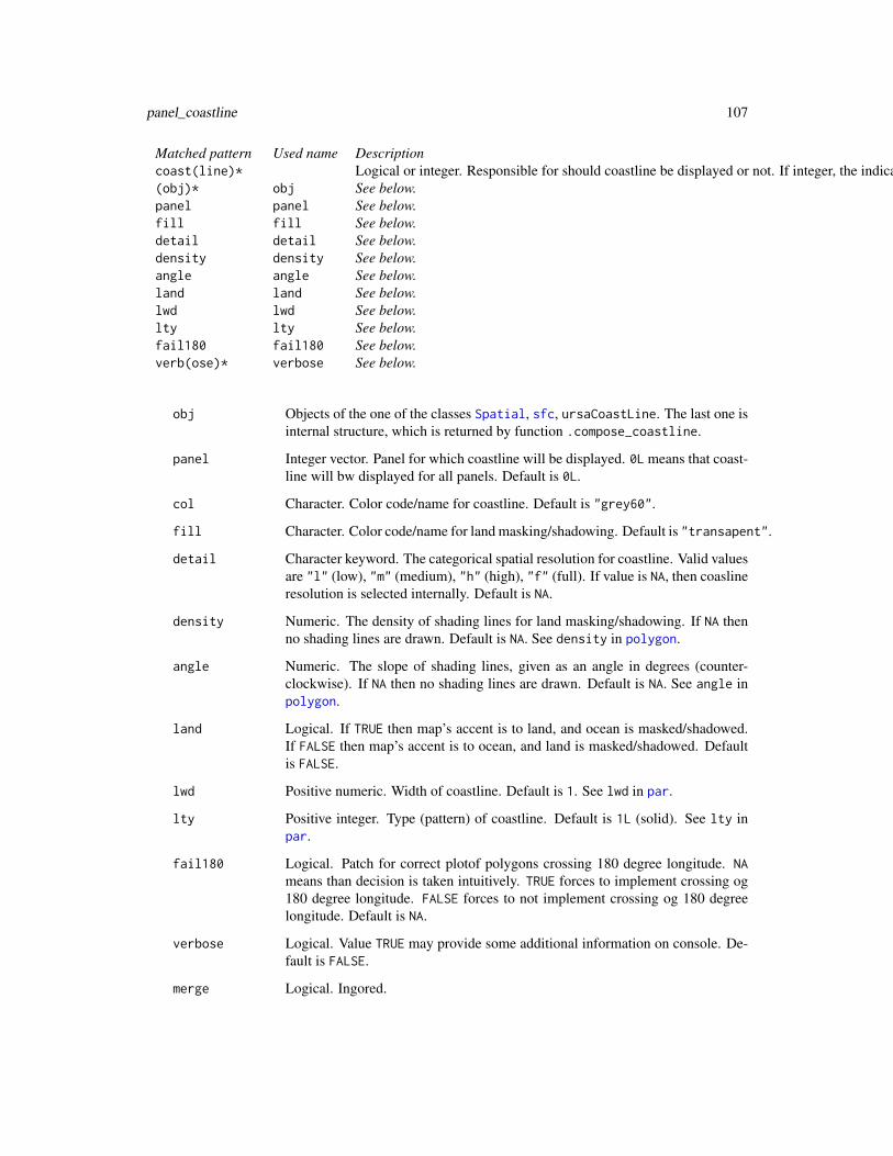
panel_coastline 107

Matched pattern Used name Descriptioncoast(line)* Logical or integer. Responsible for should coastline be displayed or not. If integer, the indicates panel index for coastline displaying. If TRUE then coastline is plotted. If FALSE then coastline is not displayed. Default is TRUE.(obj)* obj See below.panel panel See below.fill fill See below.detail detail See below.density density See below.angle angle See below.land land See below.lwd lwd See below.lty lty See below.fail180 fail180 See below.verb(ose)* verbose See below.

obj Objects of the one of the classes Spatial, sfc, ursaCoastLine. The last one isinternal structure, which is returned by function .compose_coastline.

panel Integer vector. Panel for which coastline will be displayed. 0L means that coast-line will bw displayed for all panels. Default is 0L.

col Character. Color code/name for coastline. Default is "grey60".

fill Character. Color code/name for land masking/shadowing. Default is "transapent".

detail Character keyword. The categorical spatial resolution for coastline. Valid valuesare "l" (low), "m" (medium), "h" (high), "f" (full). If value is NA, then coaslineresolution is selected internally. Default is NA.

density Numeric. The density of shading lines for land masking/shadowing. If NA thenno shading lines are drawn. Default is NA. See density in polygon.

angle Numeric. The slope of shading lines, given as an angle in degrees (counter-clockwise). If NA then no shading lines are drawn. Default is NA. See angle inpolygon.

land Logical. If TRUE then map’s accent is to land, and ocean is masked/shadowed.If FALSE then map’s accent is to ocean, and land is masked/shadowed. Defaultis FALSE.

lwd Positive numeric. Width of coastline. Default is 1. See lwd in par.

lty Positive integer. Type (pattern) of coastline. Default is 1L (solid). See lty inpar.

fail180 Logical. Patch for correct plotof polygons crossing 180 degree longitude. NAmeans than decision is taken intuitively. TRUE forces to implement crossing og180 degree longitude. FALSE forces to not implement crossing og 180 degreelongitude. Default is NA.


merge Logical. Ingored.

108 panel_coastline

Details

compose_coastline forms an obect of class ursaCoastLine. panel_coastline displays objectof class ursaCoastLine. It is expected higher performance for multi-panel plotting.

If obj is NULL, then internal data is used. This data is based on simplified polygons of OpenStreetMap-derived data. Source data is licensed under the Open Data Commons Open Database License(ODbL). The crossing longitude 180 degrees polygons are merged. Removing of small polygonsand simplifying of polygons geometry is applied for three levels of details ("l" - low, "i" - interim,"h" - high). For the full ("f") level of details data simplification is not applied.

Coastline data are taken from directory, which is specified by getOption("ursaRequisite") withdefault value system.file("requisite",package="ursa"). Package contains data of "l" (low)details level in the file system.file("requisite/coast-l.rds",package="ursa"). Data ofhigher levels can be added using update_coastline() function. It is required to specify user’srequisite path using options(ursaRequisite=path/to/user/files) before loading ursa, e.g.in the user’s ~/.Rprofile file. Otherwise, there is a chance that data can not be updated due to’permission deny’ of the system directories. Package sf and some it’s suggestions are required fordata update.

If detail=NA then the spatial resolution is selected using CRS boundary and resolution using intu-itive approach. If package’s database cannot supply required details, then lower resolution is used.

Source coastline data in EPSG:4326 are transformed to CRS projection, extracted using session_gridfunction. Coastlines with optional filling of either land or ocean area is interpreted as polygons. Iffilling is solid (there is no transparency or shading lines (numerical values of arguments densityand angle), then coastline plotting is imlemented via polypath function, otherwise polygon func-tion.

Value

panel_coastline returns NULL

compose_coastline returns of object of class ursaCoastLine. It is a list:

coast_xy Two-column matix of coordinates in the sessional projection. The polygons areseparated by c(NA,NA) rows.

panel Integer. Panel for coastline displaying. If 0L, then coastline is displayed on eachpanel.

col See description of argument col.

fill See description of argument fill.

shadow If filling is semi-transparent, then it is "alpha" of filling color (argument fill).

land See description of argument land.

density See description of argument density.

angle See description of argument angle.

lwd See description of argument lwd.

lty See description of argument lty.

License

Coastal data (land polygons) is distributed under ODbL.

https://osmdata.openstreetmap.de/data/land-polygons.html

https://osmdata.openstreetmap.de/data/land-polygons.html

https://osmdata.openstreetmap.de/info/license.html

panel_contour 109

Note

In the versions <=3.7-19 package ursa contained land polygons based on union of "GSHHS_l_L1.shp"and "GSHHS_l_L5.shp" data from Self-consistent Hierarchical High-resolution Geography Database(GSHHG), Version 2.3.3 (01 November 2014), distributed under the Lesser GNU Public License,Version 3 (29 June 2007).

Author(s)


Examples

session_grid(NULL)a <- pixelsize()p1 <- colorize(a[a>500],ramp=FALSE,interval=TRUE)p2 <- colorize(a,ramp=FALSE,pal=colorRampPalette(c("grey40","grey100"))

,verbose=!TRUE,interval=TRUE)compose_open(layout=c(2,2),legend=list(list(1,"right"),list(2,"left")))for (i in 1:4) {

panel_new(col=ifelse(i==2,"white",NA))if (i %in% c(3,4))

panel_raster(p1)else if (i %in% 2)

panel_raster(p2)if (i==1)

panel_coastline()panel_coastline(coast=4,col="#007F00",fill="lightgreen",land=TRUE)panel_coastline(coast=3,col="#0000003F",fill="#0000003F")panel_coastline(coast=2,col="black",fill="black",density=20

,angle=c(-45,45),lwd=0.25,detail="l")# panel_graticule(decor=4)panel_annotation(text=as.character(i))if (i==1)

panel_annotation(pos=c(1,1),text="default")else if (i==2)

panel_annotation(pos=c(0,1),text="greyscale")else if (i==3)

panel_annotation(pos=c(1,1),text="land is shadowed")else if (i==4)

panel_annotation(pos=c(0,1),text="ocean is masked")}compose_legend(p2,p1)compose_close()

panel_contour Add colored contour to the image panel

https://www.soest.hawaii.edu/pwessel/gshhg/

110 panel_contour

Description

An instrument to overlay multiple rasters on the same image panel. Contour is derived from oneband of raster image. The colors (and respective colorbar in legend) is an alternative to contourlabeling.

Usage

panel_contour(obj, type = "", ...)

Arguments

obj Object of class ursaRaster or NULL. Raster band for contouring. If NULL thencontour is not displayed. Default is NULL.

type Character. Keyword list to descibe characteristics of contour, which is inter-preted using regular expressions."label" specifies displaying labels on contour lines."line" specifies displaying contour lines."colo(u)*r" specifies displaying colored contour lines."fill" specifies displaying filled contour lines.Keywords can be combined in a single character, e.g., "fill label" specifiesdisplaying filled contours with labels.

... Set of arguments, which are recognized via their names (using regular expres-sions) and classes:bg Character. Color name or code for contour border. Used for contrast increas-

ing. Semi-transparency and transparency ("transparent") are allowed.Default is "black".

lwd(\\.fg)* Positive numeric. Width of contour line. Default is 1.lwd\\.bg Poistive numeric. Width of the back of contour line. For bordering

shoould exceed foreground width (argument lwd). Default is lwd*1.5.lty Numeric of character. Line type for contour. Default is 1.(lab)*cex Numeric. Character expansion factor for labels. Default is 0.85.method Character. Argument, which is passed to contour. Default is "flattest".expand Numeric. Scale factor (>=1) to artificial increasing contour details by

means of smoothing of increased image size. Not applicable for imageswith color tables. Default is NA; smoothing is determined intuitively.

before Logical. Should image reclassification be done before smoothing? De-fault is FALSE for categorical images and TRUE for numerical images.

cover Numeric. Argument, which is passed to regrid to control NA valuesduring smoothing. Default is NA; connected to default value of argumentcover in function regrid.

short Positive integer. Minimal number of points in segments for displaying.Prevents displaying very short segments in the case of high-detailed image.Default is 0: all segments are displayed.

panel_contour 111

verb(ose)* Logical. Value TRUE may provide some additional informationon console. Default is FALSE. Other arguments are used in the functuioncolorize to produce color tables.

Details

Function contourLines is used for contouring.

The color table of input raster image is kept. The output panel have one element left, becausecontours are borders between areas of the same color. It is recommended to use only gradientpalettes.

The color table is forced not to be ramp (argument ramp=FALSE in the function colorize) to preventextra density of contour lines.

The color table is forced to be interval (argument interval=1L in the function colorize) to preventlost of elements in the palette.

Value

Object of class ursaColorTable, which then should be used as an input argument for the colorbarlegend (function legend_colorbar). If there is no argument of class ursaRaster then functionreturns NULL value.

Author(s)


See Also

contourLines

contour

Examples

session_grid(NULL)a <- pixelsize()refval <- seq(450,650,by=25)val <- refval[seq(refval) %% 2 == 1]ref <- colorize(a,breakvalue=refval,pal.rich=45,pal.rotate=0)p1 <- colorize(a,breakvalue=val,pal.rich=135,pal.rotate=0)p2 <- colorize(a,breakvalue=val,pal.rich=-15,pal.rotate=0)p3 <- colorize(a,value=refval)if (exam1 <- FALSE) { ## to avoid 'Examples with CPU or elapsed time > 10s'

compose_open(legend=list(list(1,"left"),list(1,"right")),scale=2)panel_new()# ct1 <- panel_raster(ref)# ct2 <- panel_contour(p2,"colored line",palname="Greens",lwd=15,lwd.bg=0)ct2 <- panel_contour(p2,"colored line",pal.rich=240,pal.rotate=0,lwd.fg=15,lwd.bg=0)# panel_contour(ref,lwd=0)# mysource("contour.R")# mycontour(.panel_contour(a),lwd=0)if (exists("ct1"))

112 panel_contour

compose_legend(ct1,units="raster")if (exists("ct2"))

compose_legend(ct2,units="contour")compose_close(bpp=8)

}if (exam2 <- TRUE) {

compose_open(layout=c(2,2),byrow=FALSE,legend=list(list(1,"left"),list("bottom",1)

,list(1,"right"),list("top",2),list(2,"right"),list("bottom",2)))

panel_new()panel_raster(ref)panel_contour(a)panel_new()ct0 <- panel_contour(a,"color",value=val,pal.rich=240,pal.rotate=0,lwd=11,lwd.bg=12)panel_contour(a)panel_annotation(text="no colortable")panel_new()panel_raster(p1)ct1 <- panel_contour(p1,"color",lwd=11,lwd.bg=2)panel_contour(a)panel_annotation(text="colortable:category")panel_new()panel_raster(p2)ct2 <- panel_contour(p2,"color",lwd=11,lwd.bg=2)panel_contour(a)#,cex=0.5)panel_annotation(text="colortable:interval")compose_legend(ref,units="reference")compose_legend(ct0,units="contour")compose_legend(p1,units="raster")compose_legend(ct1,units="contour")compose_legend(p2,units="raster")compose_legend(ct2,units="contour")compose_close()

}if (exam3 <- TRUE) {

s <- 29session_grid(NULL)a <- as.ursa(volcano)if (FALSE) {

display(a)a2 <- regrid(a,mul=s,cascade=TRUE,verbose=TRUE)display(a2)session_grid(a)

}compose_open() ## device="windows")panel_new()ct1 <- panel_raster(a,ramp=FALSE,interval=TRUE)ct2 <- panel_contour(a,"label")rm(ct2)panel_decor()if (exists("ct2"))

legend_colorbar(ct2)

panel_decor 113

else if (exists("ct1"))legend_colorbar(ct1)

compose_close()}

panel_decor Add auxiliary elements to the plotting panel.

Description

panel_decor adds over plot sequentially the followed elements: coastline, gridline, scalebar. Un-like panel_decor, function layout.grid does not add scalebar.

Usage

panel_decor(...)

Arguments

... Passed to sequence of plotting functions:

• panel_graticule. To distinguish the same argument names in differentfunctions it is provided to use prefix “grid.*”, e.g., grid.col="grey40".

• panel_coastline. To distinguish the same argument names in differentfunctions it is provided to use prefix “coast.*”, e.g., coast.col="grey60".

• (not applicable for layout.grid) panel_scalebar. To distinguish thesame argument names in different functions it is provided to use prefix“scalebar.*”, e.g., scalebar.col="black".

Details

The sequence of elements is constant. To change order, use direct calling of panel_graticule,panel_coastline, panel_scalebar in any sequence.

Sometimes, for rasters with NA values the followed sequence may be used:

panel_coastline(col="transparent",fill="grey80")panel_raster(a)panel_coastline(col="grey40")

Value

panel_decor returns NULL value.layout.grid returns NULL value.

Author(s)


114 panel_graticule

Examples

session_grid(NULL)a <- ursa_dummy(nband=1,min=0,max=100)a[a<30] <- NAcompose_open()panel_new()ct <- panel_raster(a)panel_decor(graticule.col="green4",graticule.lwd=2,scalebar.col="brown")compose_legend(ct)compose_close()

panel_graticule Add latitude/longitude or metric grid to the image panel.

Description

panel_graticule puts a grid on the panel with raster image. If CRS is georeferenced then grid isgenerated from longitudes and latitudes.

Usage

panel_graticule(...)

compose_graticule(...)

# non-public.compose_graticule(panel = 0L, col = "grey70", border = "grey70", lon = NA, lat = NA,

lwd = 0.5, lty = 2, marginalia = rep(FALSE, 4), trim = FALSE,language = NA_character_, cex = 0.75, verbose = FALSE)

# non-public.panel_graticule(obj, marginalia = rep(TRUE, 4), verbose = FALSE)

Arguments


Matched pattern Used argument Description(graticule|grid(line)*) Logical. Responsible for should grid lines be displayed or not. If TRUE then grid lines are plotted. If FALSE then grid lines are not displayed. Default is TRUE.^(graticule|grid(line)*)$ panel See below.(graticule|grid(line)\.)*col col See below. Default value in compose_graticule depends on panel background color, "#0000002F" for ligth panel background, and "#FFFFFF4F" for dark panel background.(graticule|grid(line)\.)*border border See below. Default value in compose_graticule depends on figure background color, "#0000002F" for ligth figure background, and "#FFFFFF4F" for dark figure background.(graticule|grid(line)\.)*lon lon See below.(graticule|grid(line)\.)*lat lat See below.(graticule|grid(line)\.)*lwd lwd See below.(graticule|grid(line)\.)*lty lty See below.

panel_graticule 115

(decor|margin(alia)*) marginalia See below. .compose_graticule and .panel_graticule don’t validate correctness of this parameter.((graticule|grid(line)\.)*trim trim See below.(graticule|grid(line)\.)*language language See below.(graticule|grid(line)\.)*verb(ose)* verbose See below.

obj Objects of the class ursaGridLine. It is internal structure, which is returned byfunction .compose_graticule.

panel Integer vector. Panel for which coastline will be displayed. 0L means that coast-line will bw displayed for all panels. Default is 0L.

col Character. Color code/name for grid lines. Default is "grey70".

border Character. Color code/name for marginal labels and ticks. Default is "grey70".

lon Numeric vector. Set of longitudes for grid. If NA then set of logitudes is formedinternally. Default is NA.

lat Numeric vector. Set of latitudes for grid. If NA then set of latidudes is formedinternally. Default is NA.

lwd Positive numeric. Width of grid line. Default is 0.5. See lwd in par.

lty Positive integer. Type (pattern) of grid line. Default is 2 (dashed). See lty inpar.

marginalia Logical or integer vectors. Responsible for whether longitudes and latitudes (ormetric coordinates) be labelled on the frame of panel with raster image. If logi-cal and TRUE, then labels will be displatyed on each open side of panel. If logicaland FALSE then labels will not be displayed. If logical of length 4, then labelswill be displayed on specific side, where side index is c(bottom,left,top,right)(see description for marginal parameters in par). If argument is a vector of pos-itive integers, then labels for grid lines are plotted only for the specified pan-els, which sequence is defined in compose_design function and returned fromgetOption("ursaPngLayout")$layout. Default is c(TRUE,TRUE,TRUE,TRUE).

language Character. Language for longitude and latitude captions. If "ru" then captionsare in Russian else in English. Default is NA.

trim Logical. If grid lines are labelled then trim=TRUE prevents crossing the labelson neighbor perpendicular sides.

cex Positive numeric. The relative font size for grid lines’ labels. Make sence in thecase of labels plotting. Default is 0.75.


Details

If not language="ru" but environmental variable LANGUAGE=ru then labels are in Russian (cyrillics).

Argument gridline (or, grid) is introduced for unconditional calling of panel_graticule insideof high-level functions.

Grid lines can be controlled in high-level plot functions (e.g., display, compose_plot, display_stack,display_brick, display_rgb, etc.). To prevent displaying grid lines, use argument gridline=FALSE

116 panel_graticule

(or grid=FALSE). To display grid lines, use argument gridline=TRUE (or grid=TRUE) and pre-fix grid(line)* (gridline.* or grid.*) for grid lines’ parameters, e.g., gridline.verb=TRUE,grid.col="black". If prefix is omitted then arguments with the same names affect in other func-tions in the part of high-level function.

If grid lines are formed internally, then desirable number of lines for each direction is 3. The designof line density is based on intuition, providing pretty labelling.

If CRS is georeferenced then grid lines are corresponded to longitudes and latitudes. Integer minutesare used to illustate fractional values of degrees. If precision of minutes is insufficient, then integervalues of seconds are introduced. The fractional values of seconds are not used.

Labels are located at the points, where grid lines cross plot margin. Labels are not overlapped alongthe same side. To prevent overlapping along the same side, labels are shifted or omitted. Argumenttrim=TRUE prevents overlapping labels from neighbor sides via hidding.

Value


Author(s)


Examples

session_grid(NULL)## Changing of environmental variables is out of CRAN Policy

## Not run: Sys.setenv(LANGUAGE="ru")

# example no.1cl <- compose_design(layout=c(2,2),legend=NULL)session_grid(regrid(lim=3.2*1e6*c(-1,-1,1,1)))compose_open(cl)for (i in 1:4) {

panel_new()panel_coastline()panel_graticule(decor=TRUE,trim=i %in% c(2:4))panel_annotation(text=as.character(i))panel_scalebar(scalebar=i==3)

}compose_close()

# example no.2session_grid(regrid(lim=1e6*c(-0.5,0.5,1.5,2.5)))compose_open(layout=c(2,2),legend=NULL,skip=4)for (i in seq(getOption("ursaPngLayout")$image)) {

panel_new()panel_coastline()if (i==1)

panel_graticule()else if (i==2)

panel_new 117

panel_graticule(decor=TRUE,lon=seq(0,360,by=40)[-1],lat=seq(-90,90,by=10))else if (i==3)

panel_graticule(decor=TRUE,lon=seq(0,360,by=20)[-1],lat=seq(-90,90,by=5),trim=TRUE)

else if (i==4)panel_graticule(gridline=FALSE)

panel_scalebar(scalebar=1)panel_annotation(text=as.character(i))

}compose_close()

# example no.3 -- indirect usagesession_grid(NULL)display(pixelsize(),decor=TRUE,grid.col="green3",coast.col="darkgreen",side=2)

## Changing of environmental variables is out of CRAN Policy## Not run: Sys.setenv(LANGUAGE="") # reset environmental variable

panel_new Start plotting on the new image panel

Description

panel_new finishes plotting on previuos image panel and starts plotting on next image panel.

Usage

panel_new(...)

# non-public.panel_new(col = "chessboard", density = NA, angle = NA, lwd = 1, lty = 1,

asp = NA, mar = rep(0, 4), verbose = FALSE)

Arguments

... Set of arguments, which are recognized via their names (using regular expres-sions) and classes. Passed to non-public .panel_new. Optional prefix "blank"is used for indirect use. Separated by a dot ".", e.g., blank.fill="transparent".

Pattern (panel_new) Argument (.panel_new) Description(blank\\.)*(^$|bg|fill) col See below. Keyword "chessboard" is used by default to produce original background texture. However argument col has other default value.(blank\\.)*density density See below.(blank\\.)*angle angle See below.(blank\\.)*lwd lwd See below.(blank\\.)*lty lty See below.(blank\\.)*asp asp See below.(blank\\.)*mar mar See below.(blank\\.)*verb(ose)* verbose See below.

118 panel_new

col Character. Color code/name for panel filling/shadowing. Default is "grey80"for georeferenced images, and "grey90" for non-projected images.

density Numeric. The density of shading lines for fill/shadowing. If NA then no shadinglines are drawn. Default is NA. See density in rect.

angle Numeric. The slope of shading lines, given as an angle in degrees (counter-clockwise). If NA then no shading lines are drawn. Default is NA. See angle inrect.

lwd Positive numeric. Width of coastline. Default is 1. See lwd in rect.

lty Character or positive integer. Type (pattern) of coastline. Default is 1L (solid).See lty in rect.

asp Positive numeric. The y/x aspect ration. Default is 1. See asp in plot.window.

mar Positive numeric of length 4. Plot margins. Default is rep(0,4L). See mar inpar.


Details

Prefix blank is introduced for manipulations with panel_new inside of high-level functions (e.g.,display). Prefix skipping is the subject for confict with functions, which use the same name ofarguments.

It is required to call panel_new for every image panel. First calling starts plotting on the first panel.Second and next callings change image panels.

The panel sequence is set in function compose_design, which is called directly or indirectly fromcompose_open, and keeps in the options (access via getOption("ursaPngLayout")$layout).

Image background is formed via consecutive call of functions plot(...,type="n"), and rect(...).

Value


Author(s)


Examples

session_grid(NULL)# example no.1 -- direct usecompose_open(layout=c(1,2),legend=NULL)panel_new()panel_annotation(label="Default + Empty")panel_new(col="#0000FF3F",density=15,angle=45,lwd=3)panel_decor()panel_annotation(label="Settings + Grid")compose_close()

panel_plot 119

# example no.2 -- indirect usea <- pixelsize()a <- a[a>560]display(a,blank.col="#0000FF3F",blank.density=15,blank.angle=45,blank.lwd=3

,coast.fill="#007F005F",coast.density=20,coast.angle=c(-30,60))

panel_plot Add graphical elements to the image panel

Description

Standard fuctions for plotting from package graphics are used for manual adding elements to cur-rent plot. Theses series of functions used that standard instruments with additional controling theacceptability of plotting.

Usage

panel_plot(obj,...)

panel_box(...)panel_lines(...)panel_points(...)panel_text(...)panel_abline(...)panel_polygon(...)panel_segments(...)

Arguments

obj R object.

... In panel_plot arguments are passed to function plot.In panel_box arguments are passed to function box.In panel_lines arguments are passed to function lines.In panel_points arguments are passed to function points.In panel_text arguments are passed to function text.In panel_abline arguments are passed to function abline.In panel_polygon arguments are passed to function polygon.In panel_segments arguments are passed to function segments.

Details

If unable to get value TRUE from getOption("ursaPngPlot") then plotting is disable, and anyfunction from this series returns NULL.

Generally, for spatial objects argument add=TRUE is used in panel_plot.

120 panel_plot

Value

For spatial objects (simple features from sf or spatial abstract classes from sp) function panel_plotreturns object of class ursaLegend. It is a list with items, which can be used to as arguments oflegend(). This is intermediate step for experimental feature (not ready) to display colorbars onplot panel. For other objects function panel_plot returns value of function plot.

Function panel_box returns value of function box.Function panel_lines returns value of function lines.Function panel_points returns value of function points.Function panel_text returns value of function text.Function panel_abline returns value of function abline.Function panel_polygon returns value of function polygon.Function panel_segments returns value of function segments.

Note

For plotted elements it is possible to create legend for colors using color bars. No shapes kind andsize, no line widths.

To convert object x of class ursaLegend to object of class ursaColorTable please use ursa_colortable(x).

Author(s)


See Also

panel_contour

Package graphics (help(package="graphics")) and functions plot, box, lines, points, text,abline, polygon, segments.

Examples

session_grid(NULL)require(rgdal)a <- pixelsize()g1 <- session_grid()n <- 12Lk <- 5Lx <- with(g1,runif(n,min=minx,max=maxx))y <- with(g1,runif(n,min=miny,max=maxy))panel_plot(x,y) ## plots nothing, because 'compose_open(...,dev=F)' is not called yetsl <- lapply(seq(k),function(id){

x <- sort(with(g1,runif(n,min=minx,max=maxx)))y <- sort(with(g1,runif(n,min=miny,max=maxy)))sp::Lines(sp::Line(cbind(x,y)),ID=id)

})sl <- sp::SpatialLines(sl,proj4string=sp::CRS(ursa_proj(g1)))#,id=length(sl))lab <- t(sapply(sp::coordinates(sl),function(xy) xy[[1]][round(n/2),]))lab <- as.data.frame(cbind(lab,z=seq(k)))

panel_raster 121

sl <- sp::SpatialLinesDataFrame(sl,data=data.frame(ID=runif(k,min=5,max=9),desc=LETTERS[seq(k)]))

print(sl@data)ct <- colorize(sl@data$ID)#,name=sldf@data$desc)shpname <- tempfile(pattern = "___tmp",tmpdir=".",fileext=".shp")layername <- gsub("\\.shp$","",basename(shpname))try(writeOGR(sl,dirname(shpname),layername,driver="ESRI Shapefile"))compose_open(layout=c(1,2),legend=list(list("bottom",2)))panel_new()panel_decor()panel_lines(x,y,col="orange")panel_points(x,y,cex=5,pch=21,col="transparent",bg="#00FF005F")panel_points(0,0,pch=3)panel_text(0,0,"North\nPole",pos=4,cex=1.5,family="Courier New",font=3)panel_new()panel_decor()panel_plot(sl,lwd=4,col="grey20")if (file.exists(shpname))

panel_plot(shpname,lwd=3,col=ct$colortable[ct$index])panel_points(lab$x,lab$y,pch=as.character(lab$z),cex=2)compose_legend(ct$colortable)compose_close()file.remove(dir(path=dirname(shpname)

,pattern=paste0(layername,"\\.(cpg|dbf|prj|shp|shx)"),full.names=TRUE))

panel_raster Add raster to the image panel

Description

If specified image has 3 or 4 bands, then color composite is plotted on image panel, else the imageis plotted regarding to its color table.

Usage

panel_raster(...)

Arguments

... Set of arguments, which are recognized via their names (using regular expres-sions) and classes.1. Passed to colorize.2. interpreted in this function:

"(^$|obj)" as obj Object of class ursaRaster. Raster band for plotting. Mul-tiple bands are allowed if then can be interpreted as RGB or RGBA.

122 panel_raster

"useRaster" as useRaster Logical. If TRUE then a bitmap raster is used toplot the image instead of polygons. See argument useRaster in functionimage. Default depends on PNG device (getOption("ursaPngDevice"),which is set up in compose_open); it is TRUE for "cairo" device, and FALSEfor "windows" device.

"interp(olate)*" as interpolate Logical. Passed as argument interpolateto function rasterImage.

"(alpha|transp(aren(cy)*)*)" as alpha Numeric or character. Level oftransparency. If numeric, the either 0 <= alpha <= 1 or 0 <= alpha <= 255.If character, then one byte of hexadecimal value "00" <= alpha <= "FF".If NA, then transparency is used from colortable, else transparency of col-ortable is overwritten by alpha. Default is NA.

"verb(ose)*" as verbose Logical. Value TRUE may provide some additionalinformation on console. Default is FALSE.

Details

If obj is list of raster images, then panel_raster is applied to each item of list, and colortable oflast item is returned.

If obj has 3 or 4 bands then obj is interpreted as RGB(A) image.

Function attempts to speed up plotting by reduce image matrix for big rasters.

Value

If argument obj has strictly one band, then function returns color table - object of class ursaColorTable,which can be used as an input argument for the colorbar legend (function legend_colorbar). Oth-erwise function returns NULL value.

Author(s)


Examples

session_grid(NULL)# example no.1 -- direct usesession_grid(regrid(mul=1/32))dima <- with(session_grid(),c(columns,rows,3))a <- ursa_new(value=array(runif(prod(dima),min=127,max=255),dim=dima))p <- colorize(a,pal=c("black","white"),ramp=TRUE,value=0:256)compose_open(layout=c(2,3),skip=4,legend=list(list("top","full"),list("bottom",2:3)))for (i in seq(6)) {

panel_new()if (i<4)

panel_raster(p[i])else

panel_raster(a,interpolate=i==5)panel_decor(col="black",coast=FALSE)panel_annotation(c("red","green","blue"

,"interpolate=FALSE","interpolate=TRUE"))

panel_scalebar 123

}legend_colorbar(p,label=seq(0,256,by=16),units="channels")legend_mtext("color composite")compose_close()

# example no.2 -- indirect usedisplay(pixelsize(NULL),raster.verb=TRUE)

# example no.3 -- color table for legendsession_grid(NULL)compose_open()panel_new()ct <- panel_raster(pixelsize(),palname="Greens")panel_decor()compose_legend(ct)compose_close()

panel_scalebar Add scale bar to the image panel

Description

panel_scalebar puts a scale bar (’box’ style) on the panel with raster image.

Usage

panel_scalebar(...)

# non-public.panel_scalebar(position = "bottomleft", w = NA, cex = 0.85,

col = "#0000002F", bg = "transparent", fill = "#FFFFFF2F",language=NA, verbose = FALSE)

Arguments

... Set of arguments, which are recognized via their names (using regular expres-sions) and classes. Passed to non-public .panel_scalebar, excepting argumentscalebar:

Pattern (panel_scalebar) Argument (.panel_scalebar) Description(scalebar|ruler|decor) Logical or integer. Responsible for should scale bar be displayed or not. If logical and TRUE then scale bars are plotted on all panel of layout. If logical and FALSE then scale bars are not displayed. If argument is a vector of positive integers, then scale bars are plotted only in the specified panels, which sequence is defined in compose_design function and returned from getOption("ursaPngLayout")$layout. Default is TRUE.(scalebar\\.)*pos(ition)* position See below.(scalebar\\.)*w w See below.(scalebar\\.)*cex cex See below.(scalebar\\.)*col col See below.(scalebar\\.)*fill fill See below.(scalebar\\.)*bg bg See below.(scalebar\\.)*language language See below.(scalebar\\.)*verb(ose)* verbose See below.

124 panel_scalebar

position Character keyword or numeric of length 2 in the interval [0,1]. Defines thelocation of scale bar. If character, then one of the "bottomleft", "bottomright","topleft", "topright", "left", "right", "bottom", "top", or "center". If numeric thenrelative position on panel is defined using shift on horizontal and vertical axesfrom origin in the bottom-left corner. Default is "bottomleft".

w Positive numeric. The length in km of scalebar’s right segment. If w=NA thenlength of segment is defined automatically. Default is NA.

cex Positive numeric. The relative font size for scalebar’s labels. Default is 0.85.

col Character. Primary fill color for scalebar box and scalebar labels. Default is"#0000002F".

fill Character. Secondary fill color for scalebar box. Default is "#FFFFFF2F".

bg Character. Background color for the area of scalebar box and labels. Default is"transparent".

language Character. Language for longitude and latitude captions. If "ru" then captionsare in Russian else in English. Default is NA.


Details

The scalebar has 2 left segments and 2 right segments. Left and right segments are separated by 0.The length of left segments is a half of length of right segments.

Argument scalebar (or, synonym, ruler) is introduced for unconditional calling of panel_scalebarinside of high-level functions.

Default x=0 and y=0 define the "bottomleft" position of scale bar.

If argument scale in the function compose_open is character, then the length of one segment isexactly 1 cm, and the total length of scalebar is 3 cm.

If not language="ru" but environmental variable LANGUAGE=ru then labels are in Russian (cyrillics).

The length distortions is taken into account for transverse Mercator ("+proj=tmerc") projectionregarding to location of scalebar.

Scalebar (single occurence) can be controlled in high-level plot functions (e.g., display, compose_plot,display_stack, display_brick, display_rgb, etc.).

To plot scalebar, use argument scalebar=TRUE and prefix (ruler|scalebar) (scalebar.* orruler.*) for scalebar’s parameters, e.g., scalebar.pos="bottomright", scalebar.cex=0.9.

Scalebar is not displayed for longlat projection ("+proj=longlat"), where units are degrees.

Value


Author(s)


panel_shading 125

Examples

session_grid(NULL)# example no.1 -- direct usage

a <- colorize(pixelsize())compose_open(a)panel_new()panel_raster(a)panel_scalebar()compose_close()

# example no.2 -- indirect usagedisplay_rgb(ursa_dummy(nband=3,min=0,max=255)

,scalebar=TRUE,scalebar.col="white",scalebar.fill="black")

# example no.3 -- for paper copya <- colorize(pixelsize(),breakvalue=seq(400,650,by=50),palname="Greys",inv=FALSE)compose_open(scale="1:95000000",dpi=150,device="cairo",family="Times")compose_plot(a,gridline=FALSE,scalebar=TRUE,scalebar.x=1,units=expression(km^2))compose_close(bpp=8)

# example no.4 -- length distortion in the Transverse Mercator projectiona1 <- regrid(setbound=c(10,65,71,83),dim=c(100,100),crs=4326)a2 <- polygonize(ursa_bbox(a1))a3 <- spatial_transform(a2,3857)a4 <- regrid(setbound=spatial_bbox(a3),res=20000,crs=spatial_crs(a3))compose_open(legend=NULL)panel_new("white")panel_coastline(fill="#00000010")# panel_graticule()for (p in c("bottom","center","top"))

panel_scalebar(pos=p,w=200)compose_close()

panel_shading Shaded overlay by image mask

Description

This specific function is designed to illustrate linear slope and areas of statistically significant slopeon the same panel, however can be used commonly for shading by raster mask.

Usage

panel_shading(obj, level = NA, col = NULL, density = 25, angle = c( -45, 45),lwd = 1, lty = 1, verbose = TRUE)

126 panel_shading

Arguments


level Positive numeric. Threshold for obj reclassification { obj<(-level) | obj>(+level)}. If NULL then mask is created from non-NA values of obj. Default is NULL.

col ursaColorTable (ursaRaster with color table) or character. Color for shad-ing lines (grid). If object of class ursaColorTable.Two colors on the limits of color vector are extracted to separate source values<=(-level) and >=(+level).

density Numeric. The density of shading lines, in lines per inch. Default is 25. Seedescription of argument density in function polygon.

angle Numeric. The slope of shading lines, given as an angle in degrees (counter-clockwise). Default is vector of length two c(-45,45). See description of argu-ment angle in polygon function.

lwd Numeric. Line width for shading. Default is 1. See description of lwd in parfunction

lty Numeric or character. Line type for shading. Default is 1. See description oflty in par function.

verbose Logical. If TRUE then progresss bar is appeared. Default is TRUE.

Details

Values of input obj is reclassified to raster mask: { values<=(-level) OR values>=(+level) }.For common use, select appropriate level and, if necessary, reclassify obj prior.

Color limits are extracted using range function.

Raster images can be used for colored shading using alpha argument of panel_raster function,e.g. panel_raster(a,alpha=3/4)

Value

NULL

Author(s)


Examples

session_grid(NULL)if (first.example <- TRUE) {

session_grid(NULL)session_grid(regrid(mul=1/8))ps <- pixelsize()compose_open()ct <- compose_panel()panel_shading(ps>1.1*global_mean(ps),angle=90)compose_legend(ct)compose_close()

pixelsize 127

}if (second.example <- TRUE) {

session_grid(NULL)a <- ursa_dummy(nband=15,mul=1/8)b <- local_stat(a)compose_open()lev <- 0.90d <- as.matrix(b["slopeS"],coords=TRUE)e <- contourLines(d,levels=c(-lev,lev))p <- list(significance.raw=colorize(b["slopeS"])

,significance.formatted=colorize(b["slopeS"],stretch="significance"),slope=colorize(b["slope"]))

p <- c(p,rep(p[3],3))names(p)[c(3,4,5)] <- c("Slope and shaded significance"

,"Slope and contoured significance","Slope and 'contourLines'")

compose_open(p,layout=c(2,NA),byrow=FALSE)compose_panel(p[1])compose_panel(p[2])compose_panel(p[3])panel_shading(b["slopeS"],level=lev)compose_panel(p[4])panel_contour(b["slopeS"],value=c(-lev,lev))compose_panel(p[5])lapply(e,panel_polygon)compose_panel(p[6])ct <- panel_contour(b["slopeS"],"color"

,value=c(-0.99,-0.95,-0.9,-0.5,0.5,0.9,0.95,0.99))compose_legend(c(head(p,-1),'(Colorbar for contours)'=list(ct)),las=3)compose_close()

}

pixelsize The actual size of each grid cell with considerable distortion in areaof map projection.

Description

This function helps to calculate size of pixels in the unit of area (squared km) for zonal statisticswith taking into account distortion in area for classes of projections.

Usage

pixelsize(obj, verbose = FALSE)

Arguments

obj Either ursaRaster object or ursaGrid object or NULL or missing.


128 pixelsize

Details

pixelsize() is applied to coordinate reference system (grid) of ursaRaster object or to rastergrid directly. If argument obj is missed, then session grid is used.

Currently, only Stereographic ("+stere" in PROJ.4 notation), Mercator ("+merc"), and LambertAzimuthal Equal Area ("+laea") classes of map projections are implemented, though the last one(LAEA) has no distortion in area.

Value

Object of class ursaRaster, single-band. If size of cell is more than 10e5 square meters, then theunit is squared kilometers (band name is "Pixel Size (sq.km)") else squared meters (band name is"Pixel Size (sq.m)").

Author(s)


Examples

session_grid(NULL)pixelsize()

## internet connection is required; access was tested on 2018-06-04invisible({

dpath <- file.path("ftp://sidads.colorado.edu/pub/DATASETS","nsidc0081_nrt_nasateam_seaice/north")

dst <- tempfile(fileext=".bin")isOK <- FALSEd3 <- Sys.Date()for (i in seq(5)) {

src <- file.path(dpath,format(d3,"nt_%Y%m%d_f18_nrt_n.bin"))a <- try(download.file(src,dst,mode="wb"))if ((is.integer(a))&&(a==0)) {

isOK <- TRUEbreak

}d3 <- d3-1

}if (isOK) {

g1 <- regrid(bbox=c(-385,-535,375,585)*1e4,res=25*1e3,crs=paste("+proj=stere +lat_0=90 +lat_ts=70 +lon_0=-45"

,"+k=1 +x_0=0 +y_0=0 +a=6378273 +b=6356889.449","+units=m +no_defs"))

session_grid(g1)b <- readBin(dst,integer(),size=1L,n=136492L,signed=FALSE)ice <- ursa_new(value=tail(b,-300))ice[ice>251] <- NA ## keep Poleice[ice==251] <- 250 ## consider 100% ice at Poleice <- ice/2.5 ## uncategorizeice[ice<15] <- 0 ## not ice, if less 15%ice[ice>0] <- 100

plot 129

extent1 <- band_sum(ice*1e-2*ursa(ice,"cell")^2*1e-6)*1e-6extent2 <- band_sum(ice*1e-2*pixelsize(ice))*1e-6message(paste("Near real-time Arctic sea ice extent (NASA Team algorithm, NSIDC)"))message(sprintf(" Direct area calculation: %5.2f*1e6 km^2.",extent1))message(sprintf(" Distortion in area is corrected: %5.2f*1e6 km^2.",extent2))

}else

message("It is failed to get sea ice concentration data.")})

plot Simple display of raster images

Description

Function image for ursaRaster object calls generic function image.Function plot for ursaRaster object calls function filled.contour.Color tables are supported.

Usage

## S3 method for class 'ursaRaster'plot(x, ...)

## S3 method for class 'ursaRaster'image(x, ...)

Arguments


... Other parameters. Are passed to or filled.contour or to generic functionimage.

Details

Usage of both these functions is justified for low-level control of plotting. It is recommended to usehigh-level function display. It is flexible and power instrument for raster images visualization.

Function as.list for ursaRaster object transforms single band of raster image to a suitable objectfor plotting via function image from package graphics

Value

Returned value from image or filled.contour (both functions are in the package graphics)

Author(s)


130 polygonize

See Also

display

Examples

session_grid(NULL)a <- pixelsize()plot(a,asp=1)image(a,asp=1)b <- colorize(a,ncolor=15)plot(b,asp=1)image(b,asp=1)

polygonize Raster to vector (polygon) conversion.

Description

Representing each raster cell as a polygon. In comparison to common GIS raster to vector conver-sion, where neighbor cells with the same value are combined to the single polygon, the number ofoutput polygons is equal to number of non-NA values.

Usage

polygonize(obj, fname, engine = c("native", "sp", "sf"), verbose = NA, ...)

Arguments

obj Object of class ursaRaster.fname Missing or character. If specified, then ESRI Shapefile is created. Default is

missing.engine Character keyword from list c("native","sp","sf"). Define package with

tools for creating spatial data. If engine="sp", then functions from packagesp are used. If engine="sf", then functions from package sf are used. Ifengine="native", then appropriate package is used based on loaded names-paces before.

verbose Logical. If TRUE then convertion is attended by progress bar. Default is NA; itmeans TRUE for engine="sp" and FALSE for engine="sp".

... Additional arguments, which are passed to internal function for writing ESRIShapefile.compress Logical. Should output ESRI Shapefile files be compressed by zip?

Default is FALSE.

Details

Some GIS software (e.g., QGIS) has broad tools for display vector data. Excepting choroplets, it isassumed that visualization of each cell separately is more attractive than displaying of polygons withdifferent forms, which are produced, for example, by GDAL convertion utillity gdal_polygonize.py.

https://gdal.org/gdal_polygonize.html

read_envi 131

Value

If missing fname and tools from sp then object of class "SpatialPolygonsDataFrame" (package sp).If missing fname and tools from sf then object of class "sf" with geometry of class "sfc_POLYGON"(package sf).If fname is specified, then NULL.

Note

Implementation is very slow even for moderate image size. Use progress bar (verbose=TRUE) tocontrol this process.

Author(s)


Examples

session_grid(NULL)a <- ursa_dummy(mul=1/16)a <- a[a>100]print(a)print(band_mean(a))b2 <- polygonize(a,engine="sp") ## try 'engine="sf"'print(colMeans(spatial_data(b2),na.rm=TRUE))print(ursa_bbox(a))print(spatial_bbox(b2))

read_envi Read ENVI .hdr Labelled Raster file to memory

Description

Reads all or several bands of ENVI .hdr Labelled Raster file from disk to memory.

Usage

read_envi(fname, ...)

Arguments

fname Character. Filename for ENVI .hdr Labelled Raster file.

... For read_envi: Set of arguments, which are recognized via their names (usingregular expressions) and classes. In the case of grids mismatch some arguments(e.g., resample) are passed to regrid function.

132 read_envi

(subset)* Name can be omitted. Integer or character. If integer, then indicesof bands, either positive or negative. Positive indices are for included bands,negative indices for omitted bands. If character, then either sequence ofband names or regex string. By default (subset=NULL), function reads allbands.

(ref)* Name can be omitted. ursaRaster or ursaGrid object. Reference gridfor raster image resizing. By default (ref=NULL) there is no resizing.

(nodata|ignorevalue) Numeric. Value, which is ignored. By default (nodata=NaN)igrore value is taken from ENVI metadata (*.hdr or *.aux.xml).

reset(Grid)* Logical. If TRUE, then session grid is ignored, and new sessiongrid is assigned from input file. If FALSE, then input file is nested in thesession grid.

cache Integer. Using cache for compressed files. 0L - do not use cache, 1L -use cache; any other value resets cache. Default is FALSE.

verb(ose)* Logical. Value TRUE may provide some additional information onconsole. Default is FALSE.

Details

Function read_envi is designed to one-time reading (from disk to memory) ENVI .hdr LabelledRaster file. For multiple access to disk (by chunks), use followed construction:

a <- open_envi(fname)d1 <- a[condition_1]d2 <- a[condition_2]...close(a)

In this case, the connection keeps open. The gain is more effective for compressed binary files.

Value

Object of class ursaRaster.

Author(s)


See Also

open_envi, Extract method [ for ursaRaster object, close_envi.

read_gdal uses GDAL (rgdal) to read ENVI .hdr Labelled Raster file.

Examples

session_grid(NULL)fname <- tempfile()a <- ursa_dummy()bandname(a) <- c("first","second","third")

read_gdal 133

write_envi(a,fname,compress=FALSE)

print(read_envi(fname))print(read_envi(fname,c(1,3)))print(read_envi(fname,-c(1,3)))print(read_envi(fname,c("first","third")))print(read_envi(fname,"iR"))

print(session_grid())g <- regrid(session_grid(),mul=1/2.3)b <- read_envi(fname,ref=g)print(session_grid())print(b)

envi_remove(fname)

read_gdal Read GDAL supported raster files.

Description

read_gdal creates ursaRaster object from GDAL supported raster files using functions fromrgdal packages.

Usage

read_gdal(fname, resetGrid = TRUE, band = NULL, engine = c("native", "rgdal", "sf"),verbose = FALSE, ...)

ursa_read(fname, verbose = FALSE)

Arguments

fname Character. GDAL supported raster file name.

resetGrid Logical. If TRUE then new sessional grid is based on opened raster image. De-fault is TRUE

band Character (regular expression) or integer.

engine Character. Functionality of which package is used for reading data. If partialdata (band is not NULL), then engine is "rgdal". If value is "sf" and no par-tial data reading then sf::gdal_read() is used before importing. If value is"rgdal" or partial data reading, then interaction with rgdal is used. Currently,"native" is similar to "rgdal", but in next versions behaviour can be changedto engine selection depends on which namespace has already loaded or has sug-gested package sf been installed.


... Ignored.

134 read_gdal

Details

ursa_read is simplified implementation of gdal_read.

The composite GDAL formats (e.g., NetCDF: Network Common Data Format, HDF5: HierarchicalData Format Release 5) are likely unsupported.

read_gdal uses functions from rgdal:

• GDALinfo - to get raster metadata.

• getRasterData - to get raster data.

Category names and color tables are supported.

Value


Author(s)


See Also

rgdal::GDALinfo() for supported GDAL raster formats

as.ursa is an alternative call for GDAL raster files import.

Examples

session_grid(NULL)

rgdal::gdalDrivers()Fin1 <- system.file("pictures/Rlogo.jpg",package="rgdal")a1 <- read_gdal(Fin1)print(a1)display(a1)

Fin2 <- system.file("pictures/test_envi_class.envi",package="rgdal")b1 <- read_gdal(Fin2)b2 <- read_envi(Fin2,resetGrid=TRUE)print(identical(ursa_grid(b1),ursa_grid(b2)))print(identical(ursa_value(b1),ursa_value(b2)))print(identical(ursa_colortable(b1),ursa_colortable(b2)))print(ursa_colortable(b1))print(as.table(b1))display(b1,detail="l")

https://gdal.org/frmt_netcdf.html

https://gdal.org/frmt_hdf5.html

https://gdal.org/frmt_hdf5.html

reclass 135

reclass Reclassify specific values of image

Description

This is look-up table reclassification: the destination value is found for each source value.

Usage

reclass(obj, dst = NULL, src = NULL, sparse = FALSE, ...)

Arguments

obj Object of class ursaRaster or ursaColorTable.

dst Object of class ursaRaster, or object of class ursaColorTable, or numericvector. If numeric, then the desired destination set of values, else reference ob-ject for reclassification; this object should have numerical values of categories.

src Numerical vector, but allowed using with numerical vector of dst and length(src)==length(dst).Source set of values.

sparse Logical. If image has a lot of NA values then sparse=TRUE may speed up trans-formation. Default is FALSE.

... Other arguments are used for classification in the function colorize.

Details

If dst is numeric vector, then the source value have to be specific, without any ranges. It is requiredthe equality lengths of src and dst. If image has color table then function tries reconstruct dstfrom names of categories.

This function can be used for data compression for storage, e.g. for distribution or interchange.

Value

If obj is object of class ursaColorTable then numeric vector of categories’ centers.

If dst is numeric, then object of class ursaRaster without color table.

If dst is ursaColorTable then object of class ursaRaster (NA values) in color table.

If dst is NULL then object of class ursaRaster with empty color names (NA values) in color table.

Note

There were no a lot of tests how GIS software reads "ENVI .hdr Labelled Raster" files with colortables without color values (only categories). At least, GDAL recognizes categories (gdalinfoutility).

Author(s)


https://gdal.org/frmt_various.html#ENVI

https://gdal.org/gdalinfo.html

136 regrid

See Also

The reclassification from interval source values to specific destination values is used in colorize.

Examples

session_grid(NULL)# example no.1 manual classificationa <- as.ursa(round(matrix(runif(100,min=0.5,max=3.5),ncol=10)))print(as.table(a))b <- reclass(a,src=c(3,1,2),dst=round(runif(3),2))print(as.table(b))print(c(src=a,dst=b))

# example no.2 -- similarity to other objectsession_grid(NULL)a <- ursa_dummy(nband=2,min=-1,max=1)print(a)b1 <- colorize(a[1],value=seq(-1,1,length=21),pal.rich=240,pal.rotate=0)b2 <- reclass(a[2],b1)b3 <- reclass(a[2],ursa_colortable(b2))b <- c(b1,b2,b3)print(reclass(b))

# example no.3 -- compression with data losta <- pixelsize(NULL)b <- reclass(a,byte=TRUE,tail=0) ## try 'byte=FALSE'a2 <- reclass(b)res <- c(source=a,as_category=a2,difference=a-a2)print(res)message(paste("RMS error: ",format(sqrt(band_sum(res[3]^2)/band_n(res[3])))))prefix <- names(res)[1:2]fname <- file.path(tempdir(),paste0(prefix,".envi"))s <- data.frame(object.size=sapply(list(a,b),object.size))rownames(s) <- prefixprint(s)write_envi(a,fname[1])write_envi(b,fname[2])f <- file.info(dir(path=tempdir()

,pattern=paste0("(",prefix,")\\.(envi|hdr)",sep="|"),full.names=TRUE))[,"size",drop=FALSE]

colnames(f) <- "file.size"print(f)envi_remove(fname)

regrid Change raster image resolution and extent

Description

General function to change parameters of cells under the same geographical projection. It is imple-mented via raster resampling to the new grid.

regrid 137

Usage

regrid(x, ...)

## non-public.regrid(grid = NULL, mul = NA, res = NA, resx = NA, resy = NA, setbound = NA,

columns = NA, rows = NA, dim = NA, bbox = NA, expand = NA,minx = NA, miny = NA, maxx = NA, maxy = NA, cut = NA, proj4 = NA, crs = NA,

border = 0, zero = c("keep", "node", "center"), raster = FALSE, tolerance = NA,verbose = FALSE, ...)

Arguments


... 1. Arguments, which are passed to non-public .regrid to define parametersof new grid.

2. Set of arguments, which are recognized via their names (using regular ex-pressions) and classes:^reset(Grid)* Logical. Whether new grid will be defined as a sessional

parameter? If TRUE then returned raster defines new sessional grid. IfFALSE then session grid is not changed. Default is TRUE.

resample Logical or positive numeric. The range of aggregation in theunits of cell area. If 0 or FALSE then "nearest neighbor" value is used.The resample>0 defines the side of rectangular area in proportion tocell size; and aggregation of adjacent cells is weighted in proportionto overlapping parts of cells. Default is 1 (or, equally, TRUE); it meansthat value of output cell is weighted mean of values of overlapped inputcells in proportion of overlapping of output cell by input cells.

cover Positive numeric in the range [0,1]. The maximal fraction of NAvalues in adjusted input cells for the rule to write NA value to the outputcell. Default is 0.499.

cascade Logical. Option to get more smooth results. If TRUE and resample>2then resize function is applied sequentially with argument resample<=2.

verb(ose)* Logical. Value TRUE may provide some additional informa-tion on console. Default is FALSE.

grid Reference ursaGrid or ursaRaster object. If missing then reference grid isobtained from sessional grid session_grid()

mul numeric of length 1. Multiplication for changing image size by means of chang-ing of cell size (1/mul). mul>1 decreases cell size, mul<1 increases cell size

res numeric of length 1 or 2. New grid size by horizontal and vertical axes. Iflength is 1 then the same grid size for both axes.

resx Positive numeric of length 1. New grid size by horizontal axis.

resy Positive numeric of length 1. New grid size by vertical axis.

setbound numeric of length 4. Change units of spatial extension and define new spatialextension (boundary box) in the notation c(minx,miny,maxx,maxy).

138 regrid

columns Positive integer of length 1. Number of columns/samples in the case of defini-tion of new spatial extension (setbound is non-NA).

rows Positive integer of length 1. Number of rows/lines in the case of definition ofnew spatial extension (setbound is non-NA).

dim Positive integer of length 2. Dimenstion of raster image in the notation c(rows,columns)(or, c(lines,samples)) in the case of definition of new spatial extension (setboundis non-NA).

bbox numeric of length 4. New spatial extension (boundary box) in the notationc(minx,miny,maxx,maxy) in the same units of existing spatial extension.

minx numeric of length 1. New value for left boundary.

miny numeric of length 1. New value for bottom boundary.

maxx numeric of length 1. New value for right boundary.

maxy numeric of length 1. New value for top boundary.

cut numeric of length 4. Vector (left, bottom, right, top) in CRS units for extentexpand.

border numeric of length 1 or 4. If length 4, then vector (bottom, left, top, right) incells for extent expand. If length <4, then value is repeated for length 4.

proj4 character of length 1. New projection string in the PROJ.4 notation

crs character of length 1. The synonym to proj4.

expand numeric of length 1. Multiplier of boundary box.

raster logical. Should return blank ursaRaster object instead of ursaGrid object?See ‘Value’ section

zero character. Define central cell position relative to zero coordinates. If value is"keep", then central cell position is without changes. If value is "node", thenzero coordinates are on the crossing of cell borders. If value is "center", thenzero coordinates are in the center of central cell. Currently is not implemented.If grid is consistent, then value "keep" is used, else "node".

tolerance numeric. Threshold for comparison float point numerics. Required for internalcheck of grid consistence. Default is NA; value .Machine$double.eps multi-plied on maximal value of coordinates is used.

verbose Reporting via message about violation and restoration of coordinate grid regi-larity after non-consistence usage of parameters.

Details

Generally, argument resample sets a rectangular region. The area of this region is in proportion toarea of output cell. Argument resample is the value of this proportion. Each cell is interpreted as aset of adjoining rectangular figures. The value of output cells is a weighted mean of that input cells,which fall into rectangular region. The weights are defined as an partial area inside of rectangularregion.

Function implements "nearest neighbor" resampling method if argument resample=0 (or, resample=FALSE).If resample=1 (or, resample=TRUE) and both input and output rasters have the same cell size, thenresampling method is "bilinear interpolation".

regrid 139

Expand raster x to 3 times with cell repeating: regrid(x,mul=3,resample=FALSE) ## nearestneighbor;Expand raster x to 3 times with cell aggregation: regrid(x,mul=3,resample=TRUE) ## bilinearinterpolation;Contract raster x to 3 times without cell aggregation: regrid(x,mul=1/3,resample=FALSE) ##nearest neighbor;Contract raster x to 3 times with cell aggregation: regrid(x,mul=1/3,resample=TRUE) ## weightedmean;Low-pass filtering by 3 x 3 window size: regrid(x,resample=3*3) ## see focal_mean

However, simple contraction regrid(x,mul=1/2,resample=FALSE) is implemented as contrationwith aggregation (regrid(x,mul=1/2,resample=FALSE)), because centers or output cells are lo-cated in the nodes (crossing of boundaries of input cells).

It seems that for categorical rasters parameter resample=0 is more suitable, because nearest neig-boring does not introduce new values to output raster, excepting coincidence of input cells’ nodesand output cell centers.

Usage of proj4 argument specifies only desirable PROJ.4 string and does not do reprojection.

The violation of grid regualarity is due to columns and rows of image should be integer. Therestoration of grid regularity is realized by spatial extension (boundary box) expansion.

Value

regrid returns object of class ursaRaster.

Return value of non-public function .regrid depends on logical value of raster argument. Ifraster=FALSE then .regrid returns new grid without any change of sessional grid. If raster=TRUEthen .regrid returns blank image and changes sessional grid.

Author(s)


See Also

regrid, focal_mean

Examples

session_grid(NULL)print(g1 <- session_grid())print(g2 <- regrid(g1,mul=2))print(g3 <- regrid(g1,res=50000,lim=c(-1200000,-1400000,1600000,1800000)))print(g4 <- regrid(g1,res=50000,lim=c(-1200100,-1400900,1600900,1800100),verbose=TRUE))print(g5 <- regrid(g1,mul=1/4))print(g6 <- regrid(g1,mul=1/4,cut=c(-1,-2,3,4)*25000))print(g7 <- regrid(g1,mul=1/4,expand=1.05))print(session_grid()) ## equal to 'g1'print(a <- regrid(g1,mul=1/4,border=3,raster=TRUE))print(session_grid()) ## not equal to 'g1'

session_grid(NULL)

140 rep

'.makeRaster' <- function(nc=6,nr=8) {as.ursa(t(matrix(runif(nc*nr,min=0,max=255),ncol=nc,nrow=nr)))

}session_grid(NULL)a <- .makeRaster(12,18)expand <- 1/3a1 <- regrid(regrid(a,mul=expand,resample=FALSE),a,resample=FALSE)a2 <- regrid(regrid(a,mul=expand,resample=TRUE),a,resample=FALSE)b <- c('source'=a,'contract'=a1,'aggregation'=a2)print(b)display_brick(b,grid=TRUE

,grid.lon=(seq(ncol(a)*expand+1)-1)/expand,grid.lat=(seq(nrow(a)*expand+1)-1)/expand)

session_grid(NULL)a <- .makeRaster(6,8)expand <- 3b <- c("source"=regrid(a,mul=expand,resample=FALSE,resetGrid=FALSE)

,"simple"=regrid(a,mul=expand,cascade=TRUE,resetGrid=FALSE),"cascaded"=regrid(a,mul=expand,cascade=FALSE,resetGrid=FALSE))

print(b)display_brick(b)session_grid(a)eps <- 1e-4r <- c(0,expand^(-2)-eps,expand^(-2)+eps,1,expand^0.5

,(expand+2/3)^2-eps,(expand+2/3)^2+eps,99)g2 <- regrid(mul=expand)session_grid(g2)b <- ursa_new(bandname=sprintf("Resample=%.4f",r))for (i in seq(b))

b[i] <- regrid(a,g2,resample=r[i])print(b)display_brick(b,layout=c(2,NA)

,grid=TRUE,grid.lon=seq(ncol(a)+1)-1,grid.lat=seq(nrow(a)+1)-1)

rep Replicate bands of raster image.

Description

rep for object of class ursaRaster creates new ursaRaster objects with repitition of original bandsequence.

Usage

## S3 method for class 'ursaRaster'rep(x, ...)

Replace 141

Arguments


... Further arguments to be passed to or from other methods. Keywords:

times Positive integer. Number of times to repeat each band.

If argument has no name, then times is assumpted.

Value


Author(s)


See Also

c for ursaRaster.

Examples

session_grid(NULL)session_grid(regrid(mul=1/4))a <- ursa_dummy(nband=3)print(a)b1 <- rep(a,by=2)print(b1)b2 <- rep(a,length=5)print(b2)b3 <- rep(a[3],3)print(b3)

Replace assign values to the portion of raster images

Description

This operator is used to set or replace values in portion of bands or lines in ursaRaster object inmemory or data writing to file.

Usage

## S3 replacement method for class 'ursaRaster'x[i, j, ...] <- value

142 Replace

Arguments

x ursaRaster object

i Integer or character. If integer, then band index, specifying bands to replace. Ifcharacter, either list of band names or character sting for regular expressionto match band index. In the (spatial, temporal) interpretation of ursaRasterobject j points to temporal component.

j Mentioned for consistence with internal generic function [<-.

... Mentioned for consistence with internal generic function [<-.Use regexp=FALSE for matching by match, and regexp=TRUE for matching byPerl-compatible regexps case insensitive grep. Default is FALSE.

value ursaRaster object or numeric (scalar, matrix, array). The latter is coerced tointernal matrix of $value item of ursaRaster object.

Details

Operator \sQuote{[<-} is high-level implementation for data writing. If x$value item is not appli-cable, then value of ursaRaster is not in memory. In this case the controlled by i and j portion iswritten to file. If both i and j are missing, then x[] <-value writes values to file wholly.

It is not implemented the simultaneously writing to file portion of bands and portion of lines.

Files (currently, ENVI Binary) are opened for reading and writing.

Value

If values of ursaRaster object are in memory, then modified ursaRaster object with replacedbands or lines.If values of ursaRaster object are not applicable, then ursaRaster object as is.

Author(s)


See Also

Extract

Examples

session_grid(NULL)## Preparesession_grid(regrid(mul=1/4))a <- pixelsize()w <- c("first","second","third","fourth","fifth","sixth")b1 <- rep(a/mean(a),length(w))+seq(length(w))-1bandname(b1) <- wnr <- ursa_rows(b1)bottom <- (as.integer(nr/2)):nrwrite_envi(b1,"tmp1",compress=FALSE,interleave="bil")b2 <- b1

segmentize 143

print(b1)

## Replaceb2[1] <- 10+b1["second"]b2[2] <- 20try({

data(volcano)b2[3] <- 30+volcano

}) ## error: unable to coerceb2["fourth"] <- 40+as.matrix(b1[3])b2[5] <- 50+as.array(b1[4])set.seed(352)b2["six"] <- 60+6+runif(5,min=-1,max=1) ## only first value is used (66.42849)print(b2)print(object.size(b2))

## Writeb3 <- create_envi(b2,"tmp2")print(object.size(b3))for (i in chunk_line(b3,0.04)){

b3[,i] <- b2[,i]+100if (5 %in% i)

print(object.size(b3))}close(b3)print(object.size(b3))b4 <- read_envi("tmp2")print(b4)envi_remove("tmp[12]")

segmentize Create segmented line from points’ sequence

Description

Connect sequence of points (locations) by direct lines (tracks)

Usage

segmentize(obj, connect=c("consequent", "united"))

Arguments

obj Simple feature (package sf) or Spatial abstract class (package sp) with POINTSspatial geometry.

connect Structure of output segments; either sequence of single segments ("consequent")or single multi-segment ("united").

144 seq

Details

Function generates n-1 segments from n input points. Data (attribute table) is trasfered to outputobject with excluding of first row.

Value

Simple feature (package sf) or Spatial abstract class (package sp) with LINESTRING spatial ge-ometry.

Author(s)


Examples

session_grid(NULL)n <- 15lon <- rev(sort(runif(n,min=40,max=60)))lat <- sort(runif(n,min=30,max=50))pt <- data.frame(lon=lon,lat=lat,value=seq(n))sp::coordinates(pt) <- c("lon","lat")sp::proj4string(pt) <- "+proj=longlat"ct <- ursa_colortable(colorize(pt$value))tr <- segmentize(pt)session_grid(pt,expand=1.1)compose_open(2)panel_new()panel_plot(pt,col=ct)panel_decor()panel_new()panel_plot(tr,col=ct,lwd=3)panel_decor()compose_legend(ct)compose_close()

seq Sequence Generation for raster image and coordinate grid

Description

Set of functions to generate regular sequences of bands, x-/y-cordinates and columns/rows.

Usage

## S3 method for class 'ursaRaster'seq(...)

## S3 method for class 'ursaGrid'seq(...)

seq 145

ursa_seqx(obj)ursa_seqy(obj)ursa_seqc(obj)ursa_seqr(obj)

Arguments

... Set of arguments, which are recognized via their names (using regular expres-sions), position and classes.

.* First argument (position 1). Object of classes ursaRaster, ursaGrid.

.* Second argument (position >1). One-character name. Valid values are in thelist c("z","x","y","c","r","lines","samples"). "c" ("samples") and"r" ("lines") specify to generate cell sequence in the horizontal and ver-tical directions from bottom-left corner, whereas "z" specifies to generatesequence of bands. x and "y" return cell midpoints in spatial dimension.

obj Object of classes ursaRaster, ursaGrid. Missing obj is allowed; in this casethe session grid is considered.

Details

All ordinal sequences (axis is \dQuote{c}, \dQuote{r}, \dQuote{z}) start from 1L.axis=\dQuote{z} is ignored in the function seq for ursaGrid object. The returned value is 1L.

seq(obj) for ursaRaster objects is suitable for using in cycles across bands.

Value

Functions ursa_seqx and seq(obj,"x") return x-coordinates of cell midpoints.Functions ursa_seqy and seq(obj,"y") return y-coordinates of cell midpoints.Functions ursa_seqc, seq(obj,"samples") and seq(obj,"c") return sequence of cells in hori-zontal direction.Functions ursa_seqr, seq(obj,"lines") and seq(obj,"r") return sequence of cells in verticaldirection.Functions seq(obj) and seq(obj,"z") for ursaRaster object returns sequence of bands.Function seq(obj) and seq(obj,"z") for ursaGrid object returns 1L.

Author(s)


Examples

session_grid(NULL)session_grid(regrid(mul=1/16))print(session_grid())a <- ursa_dummy(nband=5)print(a)print(seq(a))print(seq(a,"c"))

146 session

print(seq(a,"x"))print(ursa_seqx())

session Get and set sessional parameters for grid, CRS, external software foropen PNG files.

Description

session_grid without arguments returns current grid properties. session_grid with argumentsspecifies grid, which is used by functions of this package, e.g., for plotting, for opened and createdraster images during current session.

session_pngviwer is used to permit external software to open PNG files.

session_tempdir specifies directory for temporal files in some cases.

session_use_experimental_functions allows to use undocumented (experimental) functions.

Group of functions session_proj4, session_crs, session_cellsize, session_bbox extractscertain properties of sessional grid.

Usage

session_grid(obj, ...)session_proj4()session_crs()session_cellsize()session_bbox()session_dim()

session_pngviewer(allow = NA)session_tempdir(dst = character())session_use_experimental_functions()

Arguments

obj Either missing, or NULL, or file name, or object of class ursaRaster, or objectof class ursaGrid, or spatial object (simple features (sf), spatial abstracts (sp)).

allow Logical. If TRUE then it is allowed to use external software for viewing PNGfiles. NA is interpreted as TRUE in the case of "Rscript" usage, and interpreted asFALSE in the case of interactive session or "R CMD BATCH" usage. Default isNA.

dst Character. Directory name for temporal files. Empty character or non-characteris interpreted as getwd() in the case of "Rscript" usage, and interpreted astempdir() in the case of interactive session or "R CMD BATCH" usage. De-fault is character() (empty character).

... Optional arguments passing to regrid at first.

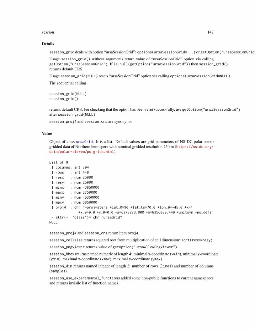
session 147

Details

session_grid deals with option “ursaSessionGrid”: options(ursaSessionGrid=...) or getOption("ursaSessionGrid").

Usage session_grid() without arguments return value of “ursaSessionGrid” option via callinggetOption("ursaSessionGrid"). If is.null(getOption("ursaSessionGrid")) then session_grid()returns default CRS.

Usage session_grid(NULL) resets “ursaSessionGrid” option via calling options(ursaSessionGrid=NULL).

The sequential calling

session_grid(NULL)session_grid()

returns default CRS. For checking that the option has been reset successfully, use getOption("ursaSessionGrid")after session_grid(NULL)

session_proj4 and session_crs are synonyms.

Value

Object of class ursaGrid. It is a list. Default values are grid parameters of NSIDC polar stereogridded data of Northern hemispere with nominal gridded resolution 25 km (https://nsidc.org/data/polar-stereo/ps_grids.html).

List of 9$ columns: int 304$ rows : int 448$ resx : num 25000$ resy : num 25000$ minx : num -3850000$ maxx : num 3750000$ miny : num -5350000$ maxy : num 5850000$ proj4 : chr "+proj=stere +lat_0=90 +lat_ts=70.0 +lon_0=-45.0 +k=1

+x_0=0.0 +y_0=0.0 +a=6378273.000 +b=6356889.449 +units=m +no_defs"- attr(*, "class")= chr "ursaGrid"

NULL

session_proj4 and session_crs return item proj4.

session_cellsize returns squared root from multiplication of cell dimension: sqrt(resx*resy).

session_pngviewer returns value of getOption("ursaAllowPngViewer").

session_bbox returns named numeric of length 4: minimal x-coodrinate (xmin), minimal y-coordinate(ymin), maximal x-coordinate (xmax), maximal y-coordinate (ymax).

session_dim returns named integer of length 2: number of rows (lines) and number of columns(samples).

session_use_experimental_functions added some non-public functions to current namespacesand returns invisile list of function names.

https://nsidc.org/data/polar-stereo/ps_grids.html

https://nsidc.org/data/polar-stereo/ps_grids.html

148 spatial_engine

Author(s)


See Also

Class ursaGrid. Use regrid to partial grid changing.

Examples

session_grid(NULL)getOption("ursaSessionGrid") ## NULL(g1 <- session_grid()) ## defaultg1$resx <- g1$resy <- 12500g1$columns <- as.integer(with(g1,(maxx-minx)/resx))g1$rows <- as.integer(with(g1,(maxy-miny)/resy))session_grid(g1)session_grid(NULL)a <- ursa_new(value=3)session_grid(a)

print(session_pngviewer())

spatial_engine Wrapper functions for manipulation with non-raster spatial objects

Description

These wrappers return iniform properties or do consimilar manipulations for spatial objects of dif-ferent types: simple features (package sf) and abstract class Spatial (package sp). Appropriatefunctionality (“engine”) of respective packages is used.

Usage

spatial_engine(obj, verbose = FALSE)

spatial_crs(obj, verbose = FALSE)spatial_proj(obj, verbose = FALSE)spatial_proj4(obj, verbose = FALSE)

spatial_crs(obj, verbose = FALSE) <- valuespatial_proj(obj, verbose = FALSE) <- valuespatial_proj4(obj, verbose = FALSE) <- value

spatial_bbox(obj, verbose = FALSE)spatial_bbox(obj, verbose = FALSE) <- value

spatial_data(obj, subset= ".+", drop = NA, verbose = FALSE)spatial_data(obj, verbose = FALSE) <- value

spatial_engine 149

spatial_geometry(obj, verbose = FALSE)spatial_geometry(obj, verbose = FALSE) <- value

spatial_geotype(obj, each = FALSE, verbose = FALSE)spatial_shape(obj, each = FALSE, verbose = FALSE)

spatial_transform(obj, crs, verbose = FALSE, ...)

spatial_coordinates(obj, verbose = FALSE)spatial_centroid(obj, verbose = FALSE)

spatial_fields(obj, verbose = FALSE)spatial_colnames(obj, verbose = FALSE)

spatial_fields(obj, verbose = FALSE) <- valuespatial_colnames(obj, verbose = FALSE) <- value

spatial_area(obj, verbose = FALSE)

spatial_dim(obj, verbose = FALSE)

spatial_count(obj, verbose = FALSE)

spatial_nrow(obj, verbose = FALSE)spatial_ncol(obj, verbose = FALSE)

spatial_filelist(path = ".", pattern = NA, full.names = TRUE, recursive = FALSE,ignore.case = TRUE)

spatial_dir(path = ".", pattern = NA, full.names = TRUE, recursive = FALSE,ignore.case = TRUE)

spatial_basename(fname)spatial_pattern(fname)

is_spatial(obj, verbose = FALSE)

is_spatial_points(obj, verbose = FALSE)is_spatial_lines(obj, verbose = FALSE)is_spatial_polygons(obj, verbose = FALSE)

spatial_intersection(x, y,geometry=c("default", "polygons", "lines", "points", "all"),verbose = FALSE)

spatial_symdifference(x, y, verbose = FALSE)spatial_difference(x, y, verbose = FALSE)spatial_union(x, y, byid=NA, verbose = FALSE)

150 spatial_engine

spatial_buffer(obj, dist = 0, quadsegs = 30L, verbose = FALSE)

spatial_trim(obj)

spatial_valid(obj, each = FALSE, reason = FALSE, verbose = FALSE)

spatial_grid(obj)

spatial_bind(...)

Arguments

obj Simple feature (package sf) or Spatial abstract class (package sp) for all func-tions, excepting spatial_geometry<-. Data frame for Replace function spatial_geometry<-.

x, y Objects of simple feature (package sf) class or Spatial abstract class (packagesp).

crs Projection EPSG code or projection PROJ.4 string.

subset Pattern to field names (colnames) of attribute table (data frame) for subbsettingusing regular expressions. By default, all fields are secected.

drop Logical. Dropping column of data frame. If TRUE, then vector of data is returned.If FALSE, then structure of data is kept. Default is NA, which is interpreted asTRUE for single column and as FALSE for multiple columns.

value Value for property assignment in replacement functions. Either numeric EPSGcode or character PROJ.4 string for spatial_crs<- and spatial_proj4<-.Spatial object or geometry of spatial object for spatial_geometry<-.

path See description of argument path in function dir.

pattern See description of argument pattern in function dir.

full.names See description of argument full.names in function dir.

recursive See description of argument recirsive in function dir.

ignore.case See description of argument ignore.case in function dir.

quadsegs Integer. Number of segments per quadrant (fourth of a circle), for all or per-feature. See description for quadsegs argument of gBuffer and for nQuadSegsargument of st_buffer.

dist Numeric. Buffer distance for all, or for each of the elements. See descriptionfor width argument of gBuffer and for dist argument of st_buffer.

byid Logical. For spatial_union function, TRUE does unite of each feature; FALSEreturns a single feature that is the geometric union of the set of features; defaultNA is coerced to FALSE for unary operation (missing y) and to TRUE for binaryoperation.

fname Character. Filename (source or packed) of spatial data.

each Logical. Whether result will be returned for each record (TRUE) or generalized(FALSE). Default is FALSE.

spatial_engine 151

geometry Character. Desired output geometry for engine="sf". If "default" then outputgeometry is defined internally (e.g., "polygons" for polygons intersection). If"all" then no output subsetting. Default is "default".

reason Logical. If TRUE, then the reason for validity ("Valid Geomerty") or invalidity isreturned. If FALSE, then logical value of validity is returned. Default is FALSE.

verbose Logical. Value TRUE provides information on console. Default is FALSE.

... 1) Spatial objects for function spatial_bind; 2) Further arguments in functionspatial_transform passed to sf::st_transform or to sp::spTransform.

Value

spatial_engine returns package name (character string "sf" or "sp"), which functionality is usedfor manipulation with spatial object obj.

spatial_crs and spatial_proj4 are synonyms, The Extract functions return projection string inthe PROJ.4 notation; the Replace functions change projection property of the object.

spatial_bbox (Extract function) returns numeric vector of length 4 with names "xmin", "ymin","xmax" and "ymax".

spatial_bbox<- (Replace function) assigns boundary bbox to the object; it is valid only for objectsof Spatial abstract class (package sp).

spatial_data (Extract function) returns attribute table only, without geometry. Subsetting fieldscan be specified by argument subset using regular expressions. If drop=TRUE and selected singlecolumn then vector is returned instead of data frame.

spatial_data<- (Replace function) adds spatial data to the object geomerty. Source data (ifpresents) are droped.

spatial_geometry (Extract function) returns only geometry, which format is depended on classof obj.

spatial_geometry<- (Replace function) addes geometry to the object.

spatial_transform does a transformation of spatial coordinates to the new CRS and returns objectof the same class as class of obj.

spatial_geotype and spatial_shape are synonyms; each returns type of spatial data: "POINT","LINESTRING", "POLYGON", "MULTIPOLYGON", . . . .

spatial_coordinates returns simplified matrix or list of coordinates of original object.

Extract functions spatial_fields and spatial_columns return column names of spatial attribu-tive table. spatial_columns is synonym to spatial_fields.

Replace functions spatial_fields<- and spatial_columns<- change column names of spatialattributive table. spatial_columns<- is synonym to spatial_fields<-.

spatial_area is valid for polygonal geometry. It returns area of polygons.

spatial_length is valid for linear geometry. It returns length of lines.

spatial_dim gets dimension of spatial coordinates; it returns either 2L (XY) or 3L (XYZ).

spatial_count returns number of items of object geometry.

spatial_nrow and spatial_ncol return number of rows and number of columns of attributivetable.

152 spatial_engine

spatial_filelist and its synonym spatial_dir return list of files with file extensions, whichare associated with certain GIS vector formats. The function’s basis is dir.

spatial_basename returns basename (without extension) of file fname of spatial object.

spatial_pattern returns pattern of spatial_basename for using in regular expressions.

is_spatial returns logical value does the object belong to the class of spatial data.

is_spatial_points returns logical value does the object have point geometry.

is_spatial_lines returns logical value does the object have (multi)linestring geometry.

is_spatial_polygons returns logical value does the object have (multi)polygonal geometry.

spatial_intersection returns intersection of two spatial objects.

spatial_difference returns difference of two spatial objects.

spatial_symdifference returns symmetric difference of two spatial objects.

spatial_buffer returns buffered spatial object.

spatial_union returns combined geometry without internal boundaries.

spatial_trim returns spatial object without extra attributes added by ursa package.

spatial_grid generates suitable spatial grid from input vector and returns object of class ursaGrid.

spatial_centroid returns spatial centroid.

spatial_bind returns spatial object concatenated from input spatial objects.

Acknowledgements

The great improvement for development of functions for manipulation with spatial objects has beenreached during work in series of projects (2015-2018) for design of marine protected areas in theArctic, which were supported by WWF Russia.

Author(s)


References

Classes and methods in packages sf and sp help.

Examples

session_grid(NULL)n <- 1e2x <- runif(n,min=25,max=65)y <- runif(n,min=55,max=65)z <- runif(n,min=1,max=10)da <- data.frame(x=x,y=y,z=z)if (requireNamespace("sp")) {

da.sp <- dasp::coordinates(da.sp) <- ~x+ysp::proj4string(da.sp) <- "+init=epsg:4326"print(spatial_bbox(da.sp))

spatial_read 153

print(spatial_crs(da.sp))}if (requireNamespace("sf")) {

da.sf <- sf::st_as_sf(da,coords=c("x","y"),crs=4326)print(spatial_bbox(da.sf))print(spatial_crs(da.sf))

}

spatial_read Wrapper functions for reading spatial objects.

Description

Read either simple features (package sf) and abstract of class Spatial (package sp) from disk usingappropriate functionality (“engine”) of respective packages is used.

Usage

spatial_read(dsn, engine = c("native", "sp", "sf"))

Arguments

dsn Character. File name of spatial object (vector GIS).

engine Character. Functionality of which package is used for reading data. If valueis "sf" then package is sf is used and simple features are returned. If value is"sp", then package rgdal is used and Spatial abstracts (package sp) are returned.If value is "native" then engine selection depends of which namespace hasalready loaded or has suggested package sf been installed.

Details

Currently, list of arguments of this funtion is simplified and can be expanded.

Value

Depending of used engine, either simple features (package sf) or Spatial abstracts (sp).

Author(s)


See Also

read_sf (valid if package sf is installed)

readOGR (package rgdal)

spatial_write

154 spatial_write

Examples

session_grid(NULL)n <- 1e2x <- runif(n,min=25,max=65)y <- runif(n,min=55,max=65)z <- runif(n,min=1,max=10)da <- data.frame(x=x,y=y,z=z)if (requireNamespace("sf",quietly=TRUE)) {

obj1 <- sf::st_as_sf(da,coords=c("x","y"),crs=4326)print(series(obj1))fname1 <- file.path(tempdir(),"res1.shp")print(fname1)spatial_write(obj1,fname1)res1 <- spatial_read(fname1,engine="sf")print(series(res1))

}if (requireNamespace("sp")) {

obj2 <- dasp::coordinates(obj2) <- c("x","y")sp::proj4string(obj2) <- sp::CRS("+init=epsg:4326")print(series(obj2))print(spatial_crs(obj2))fname2 <- file.path(tempdir(),"res2.shp")print(fname2)spatial_write(obj2,fname2)res2 <- spatial_read(fname2,engine="sp")print(series(obj2))

}print(spatial_dir(tempdir()))

spatial_write Wrapper functions for writing spatial objects.

Description

Write spatial object to disk. If spatial object is Simple Features, then appropriate functions frompackage sf are used. If spatial objest are abstract of class Spatial then appropriate functions frompackages sp and rgdal are used.

Usage

spatial_write(obj, fname, layer, driver = NA, compress = "",ogr2ogr = nchar(Sys.which("ogr2ogr")) > 0, verbose = FALSE)

Arguments

obj Spatial object: either Simple Features (sf) or Spatial Abstract (sp). List of spatialobjects can be used.

spatial_write 155

fname Character. File name with or without extension. If extension is missed, thenargument driver must be specified.

layer Character. Layer name. If missed, then basename of fname is used.

driver Character. Driver for specification of output file format. Default is NA; value isdetermined from extension of fname.

compress Character or logical. Will output file or list of files be packed after writing andwhat archive format will be used. Available character values are "" (default;no compression), "gz", "gzip", "bz2", "bzip2", "zip", "xz". If logical andTRUE, then "zip" is used for driver "ESRI Shapefile" and "gzip" otherwise. Iflogical and FALSE, then no compression.

ogr2ogr Logical. If "ogr2ogr" is found in system path, then GDAL utils are used forspeed up and layer merge (if obj is list of spatial objects)

verbose Logical. Value TRUE provides information on console. Default is FALSE.

Details

Based on sf::st_write and rgdal::writeOGR functions with additonal options: compressing ofoutput file(s), coordinates trasforming (to longitudes and latitudes for driver="GeoJSON"), creatingmulti-layer destination (for driver="SQLite").

Value

invisible NULL.

Author(s)


See Also

write_sf (valid if package sf is installed)

writeOGR (package rgdal)

spatial_read

Examples

session_grid(NULL)n <- 1e2x <- runif(n,min=25,max=65)y <- runif(n,min=55,max=65)z <- runif(n,min=1,max=10)da <- data.frame(x=x,y=y,z=z)if (requireNamespace("sf",quietly=TRUE)) {

obj1 <- sf::st_as_sf(da,coords=c("x","y"),crs=4326)print(series(obj1))fname1 <- file.path(tempdir(),"res1.shp")print(fname1)spatial_write(obj1,fname1)

156 summary

res1 <- spatial_read(fname1,engine="sf")print(series(res1))

}if (requireNamespace("sp")) {

obj2 <- dasp::coordinates(obj2) <- c("x","y")sp::proj4string(obj2) <- sp::CRS("+init=epsg:4326")print(series(obj2))print(spatial_crs(obj2))fname2 <- file.path(tempdir(),"res2.shp")print(fname2)spatial_write(obj2,fname2)res2 <- spatial_read(fname2,engine="sp")print(series(obj2))

}print(spatial_dir(tempdir()))

summary Summary of raster image.

Description

Function summary for ursaRaster object produces summaries for each band.Function summary for ursaValue object produces summaries for all values of raster image regard-less of bands.

Usage

## S3 method for class 'ursaRaster'summary(object, ...)

## S3 method for class 'ursaNumeric'summary(object, ...)

## S3 method for class 'ursaCategory'summary(object, ...)

Arguments

object Object of classes ursaRaster, ursaNumeric, or ursaCategory

... Additional arguments affecting the summary produced.

Details

summary for ursaRaster object applies summary to each column of two-dimensions value matrixand collating the results.summary for ursaValue object drops dimensions and applies summary to a vector.

temporal_interpolate 157

Value

summary for ursaRaster object returns value of function summary.matrix.summary for ursaValue object returns object of class \dQuote{summaryDefault}.

Author(s)


See Also

summary in package base.

Examples

session_grid(NULL)session_grid(regrid(mul=1/4))a <- ursa_dummy(nband=3)print(summary(a))print(summary(ursa_value(a)))print(a)

temporal_interpolate Fill gaps across bands using moving mean window

Description

temporal_interpolate is applicable for multiband raster image, where bands are regular times-tamps or period. For each cell (local operation of map algebra), NA value is replaced by averagingof two closest values (one value before, one value later) inside of moving window.

Usage

temporal_interpolate(obj, win = 7, cover = 0, verbose = FALSE)

Arguments

obj Object of class ursaRaster or matrix, where spatial locations are by rows andtemporal observations are by columns.

win Positive integer. Size of moving window. Required odd value; otherwise iscoerced to the closest odd integer.

cover Not applicable. For consistence call with temporal_mean.

verbose Logical. TRUE provides some additional information on console. Default isFALSE.

158 temporal_mean

Details

Function uses weighted averaging depending of proximity of found non-NA values. For example, ifind is temporal index of NA value in the center of movind window, indL=ind-2 is temporal indexof the closest early value valL, and indR=ind+1 is temporal index of the closest late value valR,then result is val <- (1/3) * valL + (2/3) * valR.

Value

ursaRaster object, if obj is object of class ursaRaster.

matrix object, if obj is a matrix.

Author(s)


See Also

temporal_mean

Examples

session_grid(NULL)n <- 45 # bandsm <- 3 # sample sizek <- median(seq(n))+seq(m)-(m %/% 2)-1 ## sample subsets <- 5 # window sizea <- round(ursa_dummy(n,min=-60,max=60,elements=15,mul=1/8))a[a<(-40)] <- NAb <- temporal_interpolate(a,7)p1 <- colorize(a,lazy=TRUE)p2 <- colorize(b,lazy=TRUE,colortable=p1)display(list('Source'=p1[k],'Gaps are filled'=p2[k]),layout=c(2,NA)

,legend=list(list(1,"right"),list(2,"right")),decor=FALSE)

temporal_mean Smooth value across bands using moving mean window

Description

temporal_mean is applicable for multiband raster image, where bands are regular timestamps orperiod. For each cell (local operation of map algebra), the values are averaged using moving win-dow.

Usage

temporal_mean(obj, win = 7, cover = 0, verbose = FALSE)

temporal_mean 159

Arguments

obj Object of class ursaRaster or matrix, where spatial locations are by rows andtemporal observations are by columns.

win Positive integer. Size of moving window. Required odd value; otherwise iscoerced to the closest odd integer.

cover Numeric in the interval 0 <= cover <= 1 or positive numeric >1. The requiredamount of non-NA elements in window to do a filtering. Otherwise, NA value isin output cell. If cover<=1 then amount is relative to window size. Default is 0:NA values are produced only if all elements in window have NA value.

verbose Logical. TRUE provides some additional information on console. Default isFALSE.

Details

temporal_mean is similar to function runmean(x=obj,k=win,endrule="mean") from packagecaTools.

Value

ursaRaster object, if obj is object of class ursaRaster.

matrix object, if obj is a matrix.

Advanced

temporal_mean is only smoothing of time-series. For time-series analysis and processing it issuggested to apply lower-level approach.

as.matrix (for ursaRaster object with argument coords=FALSE) or ursa_value return matrixwith spatial component by rows and temporal component by columns. It is possible to use applywith argument MARGIN=1 to this matrix. If apply returns matrix Y, then this matrix can be coercedto ursaRaster object by calling as.ursa with argument t(Y).

X <- as.matrix(obj)Y <- apply(X, 1, function(x) {y <- do_something_return_matrix(x); y})res <- as.ursa(t(Y))

For example, package caTools provides some functions for manipulation with moving window.

Author(s)


References

Package caTools https://CRAN.R-project.org/package=caTools

See Also

caTools::runmean (click if package caTools is installed)

https://CRAN.R-project.org/package=caTools

160 ursa

Examples

session_grid(NULL)set.seed(352)n <- 45 # bandsm <- 3 # sample sizek <- median(seq(n))+seq(m)-(m %/% 2)-1 ## sample subsets <- 5 # window sizea <- round(ursa_dummy(n,min=-60,max=60,elements=15,mul=1/8))

## namespace of package 'caTools' is requiredif (requireNamespace("caTools")) {

b1 <- as.ursa(t(apply(as.matrix(a),1,caTools::runmean,k=s,endrule="mean")))b2 <- temporal_mean(a,s)print(b1[k])print(b2[k])print(c('identical?'=all.equal(ursa_value(b1),ursa_value(b2))))

}

a[a<(-40)] <- NAva <- as.matrix(a) # or 'ursa_value(a)'b3 <- temporal_mean(a,s,cover=3/4,verbose=TRUE)b4 <- as.ursa(temporal_mean(as.matrix(va),s,cover=3/4,verbose=TRUE))p <- list('Before moving window'=a[k]

,'After moving window'=b3[k],'\'temporal_mean\' to matrix'=b4[k])

print(p)print(c('identical?'=all.equal(ursa_value(b3),ursa_value(b4))))display(p[1:2],legend=list(list(1,"right"),list(2,"right")),decor=FALSE)

ursa Get and set properties of raster image.

Description

For package description see.

ursa is a wrapper to initialize object of class ursaRaster, to get and to set properties for this object.

Usage

ursa(obj, attr, ...)ursa(obj, attr, ...) <- value

Arguments

obj Any numeric structure (scalar, matrix, array) for initializing. Object of classursaRaster for extracting and assigning properties.

attr Character. Name of property.... Arguments, which are passed for properties specification.value Value for property assignment.

ursa 161

Details

Initializing function ursa with missing argument attr is a wrapper for function as.ursa.

Matched pattern Replace method? Description of property Implementation"grid" Yes Raster grid (extent, projection, cellsize) ursa_grid"(proj|crs)" Yes Coordinate reference system ursa_proj"val" Yes Raster value in the internal storage format ursa_value"(colort|ct)" Yes Color table ursa_colortable"(categ|class)" Yes Names of categories names(ursa_colortable(obj))"name" Yes Band names names"(nodata|ignorevalue|bg)" Yes Value, which is interpreted as NA. ignorevalue"^table$" No Frequency of unique values as.table"cell" No Squared cell size with(ursa_grid(obj),sqrt(resx*resy))"^dim$" No Dimension of raster image dim"(extent|bbox)" No Spatial extent of raster image with(ursa_grid(obj),c(xmin=minx,ymin=miny,xmax=maxx,ymax=maxy))"(nrow|rows|lines)" No Number of rows of raster image ursa_grid(obj)$rows"(ncol|columns|samples)" No Number of columns of raster image ursa_grid(obj)$columns"con" No structure of connection obj$con"(info|meta(data)*)" No Metadata, brief info ursa_info"^file(name)*" No Connection name (filename) obj$con$fname

Argument . . . is used to specify band index or band pattern in ursa(obj,"value",...)

Value

Inititalizing function ursa (missing attr) returns object of class ursaRaster.

Extract function ursa returns object of respective property.

Replace function ursa<- returns object

Author(s)


See Also

as.ursa

Examples

a1 <- ursa(volcano)print(a1)display(a1)

a2 <- ursa(volcano,flip=TRUE)print(a2)display(a2)

a3 <- ursa(volcano,permute=TRUE)print(a3)

162 ursaConnection

display(a3)

a4 <- ursa(volcano,flip=TRUE,permute=TRUE)print(a4)display(a4)

dima <- c(200,300,4)b1 <- ursa(array(runif(prod(dima)),dim=dima))print(b1)display_brick(b1,scale=1,pal.rotate=0,pal.hue=0,decor=FALSE)

session_grid(NULL)

c1 <- ursa(seq(3))print(c1)c2 <- ursa(seq(3),bands=3)print(c2)

c3 <- ursa(value=FALSE)str(ursa(c3,"value"))

c4 <- ursa(bands=2,nodata=-99L)print(c4)print(ursa(c4,"nodata"))

c5 <- ursa(bandname=format(Sys.Date()+seq(7)-1,"%A"))ursa(c5,"value") <- rev(seq(nband(c5)))c5 <- colorize(c5)ct <- ursa(c5,"colortable")print(c5)

v <- ursa(c5[3:5],"value")str(v)v <- c(v)str(v)c6 <- ursa(v,colortable=ct)print(c6)print(ursa(c6,"colortable"))

ursaConnection Connection of raster objects.

Description

Class ursaConnection is a part of class ursaRaster. It defines storage of raster images and ma-nipulations with reading and writing.

Usage

## S3 method for class 'ursaConnection'

ursaConnection 163

print(x, ...)

## S3 method for class 'ursaConnection'seek(con, where = NA, origin = "start", rw = "", ...)

Arguments

x ursaConnection object in function print.

con ursaConnection object in function seek.

where Passed to seek for class connection.

origin Passed to seek for class connection.

rw Passed to seek for class connection.

... print: Further arguments passed to generic functions print and str.seek: Further arguments passed to function seek for class connection.

Details

ursaConnection get item $con from ursaRaster object.

Functions print and is.con are for developers rather than users.

Non-public function .con.skeleton() is used to generate the blank ursaConnection object. Thisapproach provides unified sequence of list’s items:

Value

ursaConnection is a list. The most of names have a relation to specification of ENVI Header Files.Items:

driver Character. Keyword of supported image formats. Allowed "ENVI" or "GDAL".

samples Integer. Number of image columns (samples)

lines Integer. Number of image rows (lines)

bands Integer. Number of image bands (channels, layers)

datatype Integer. Keyword for data type (4 - 32-bit floating point, 2 - 16-bit signed integer,etc)

interleave Character "bsq", "bil", "bip". Data interleave - streams of bytes in storage.

byteorder Integer, 0 or 1. The order of bytes. byteorder=0 less significant byte first,byteorder=1 most significant byte first

endian Character. See \dQuote{endian} argument in readBin and writeBin

swap Integer 0 or 1. Passed to C-funcions fread and fwrite

signed Logical. Derived from $datatype

offset Integer. Header offset in binary file. Default is 0.

wkt Logical. In ENVI Header files wkt=TRUE forced to use “coordinate systemstring” field instead of “projection info” field

nodata Numeric. Replacement NA values in the storage.


164 ursaConnection

mode Character. storage.mode of data

sizeof Integer, positive. Size in bytes for stored values. Extracted from $datatype

indexC Integer vector. Sample indices in spatial cropping.

indexR Integer vector. Line indices in spatial cropping.

indexZ Integer vector. Band indices

posC Integer vector. Sample indices in partial reading.

posR Integer vector. Line indices in partial reading.

posZ Integer vector. Band indices in spatial crottping or partial reading.

fname Character. File name. If driver=ENVI, then full path for ENVI binary file.

connection Character. See connections

compress Signed integer. 0L no compressing, -1L comressed file plus decompressedfile,-2L decompressed file, 1L - file will be compressed.

seek Logical. Does connection support seek?

handle connections in fact

Author(s)


See Also

ursa(obj,"con")

Examples

session_grid(NULL)print(methods(class="ursaConnection"))

a <- pixelsize()write_envi(rep(a,5),"tmp1",compress=FALSE)## change spatial domain for cropping exampleg <- session_grid(regrid(lim=c(-1200000,-1400000,1600000,1800000)))print(g)b <- open_envi("tmp1")d <- b[,30:70]print(ursa(d[2:3],"con"))close(b)envi_remove("tmp1")

ursaGrid 165

ursaGrid Spatial parameters of raster images.

Description

Class ursaGrid is a part of class ursaRaster. It defines spatial locations of image.

Usage

## S3 method for class 'ursaGrid'print(x, ...)

## S3 method for class 'ursaGrid'str(object, ...)

## S3 method for class 'ursaGrid'dim(x)

## S3 method for class 'ursaGrid'as.data.frame(x, row.names = NULL, optional = FALSE, ...)

Arguments

x ursaGrid object in functions print, dim and as.data.frmame.object ursaGrid object in function str.row.names Ignored. Argument, which is passed to generic function as.data.frame.optional Ignored. Argument, which is passed to generic function as.data.frame.... Further arguments passed to generic functions as.data.frame, print, and str.

Details

The blank ursaGrid object is generated by calling of ursa_grid() without arguments. Theseapproaches provide unified sequence of list’s items:

List of 9$ columns: int NA$ rows : int NA$ resx : num NA$ resy : num NA$ minx : num NA$ maxx : num NA$ miny : num NA$ maxy : num NA$ proj4 : chr ""- attr(*, "class")= chr "ursaGrid"

NULL

166 ursaProgressBar

Value

Object of class ursaGrid is a list with items:

columns Number of columns (samples)

rows Number of rows (lines)

resx Grid cell size by horizontal axis

resy Grid cell size by vertical axis

minx Left margin of boundary box

maxx Right margin of boundary box

miny Bottom margin of boundary box

maxy Top margin of boundary box

proj4 PROJ.4 string

Function dim for object of class ursaGrid returns named vector of length 2: number of rows("lines") and number of elements in a row ("samples")

Author(s)


See Also

regrid, session_grid

Examples

session_grid(NULL)print(methods(class="ursaGrid"))

a <- pixelsize()g <- ursa_grid(a)print(is.ursa(a,"grid"))print(is.ursa(g,"grid"))print(g)

ursaProgressBar Progress bar

Description

Informative progress bars with dispaying elapsed and remained time.

ursaProgressBar 167

Usage

ursaProgressBar(kind = c("tk", "txt"),title = .argv0(),label = "", min = 0, max = 1, initial = min, width = NA,style = 1, tail = FALSE, silent = FALSE)

setUrsaProgressBar(pb, value, title = NULL, label = NULL)

## S3 method for class 'ursaProgressBar'close(con, ...)

Arguments

kind Character. Type or progress bar. Valid values are "tk" to display progress barin tcl/tk window and "txt" to display progress bar in terminal mode. Default is"tk".

style See description for the same argument in txtProgressBar.

width See description for the same argument in tkProgressBar.title, label, min, max, initial, value, pb

See description for the same arguments in tkProgressBar and txtProgressBar.

con, ... See description for the same arguments in close.

tail Logical. Behaviour of progress bar appearing. If TRUE then progress bar will beused after progress step (e.g., at the end of routine). Default is FALSE (beforeprogress step).

silent Logical. If TRUE then progress bar will not appeared; it can be useful for condi-tional scripting. Default is FALSE.

Details

Wrapper to one of txtProgressBar,

tkProgressBar .

Visualization of progress bar is updates each 0.5 seconds, it is effective for multiple short-termiterations.

Progress bars should be closed by calling of appropriate method of generic function close depend-ing of class of reference progress bar.

Value

ursaProgressBar returns object of reference progress bar.

Note

Function name in style camelCase for consistence with other progress bar functions in R.

168 ursaRaster

Author(s)


See Also

txtProgressBar

tkProgressBar

Examples

session_grid(NULL)n1 <- 3n2 <- 83p <- 0.0011#require(tcltk)pb <- ursaProgressBar(min=0,max=n1,title="first",tail=TRUE)for (i in seq(n1)) {

pb2 <- ursaProgressBar(min=0,max=n2,title="second")for (i in seq(n2)) {

setUrsaProgressBar(pb2)Sys.sleep(p)

}close(pb2)setUrsaProgressBar(pb)

}close(pb)

ursaRaster Definition of ursaRaster class.

Description

ursaRaster is S3 class for manipulation with georeferred raster images. See ‘Value’ section .is.ursa checks inhering to class ursaRaster

Usage

## S3 method for class 'ursaRaster'print(x, digits = NA, grid = FALSE, raw = FALSE, caption = FALSE, ...)

## S3 method for class 'ursaRaster'str(object,...)

is.ursa(obj, ref = NULL)is_ursa(obj, ref = NULL)

ursaRaster 169

Arguments

x, object ursaRaster object.

obj Any.

digits Passed to format function

grid Logical. If grid=TRUE then returns simplified metadata.

raw Logical. If FALSE and values are categories, then attempting to restore numericvalues from categorical names is before calculating of statistics. If TRUE thenvalues for statistics are used as is. Default is FALSE.

caption Logical of character. Print title or other identificational info. If logical andTRUE then print variable name or character representation of expression. If non-zero length character, then print this value. If FALSE (default) or zero-lengthcharacter, then no header for printing.

... Passed to format function

ref Character or NULL. If character, then checking of ursaRaster sub-class(es):

Pattern DescriptionNULL ursaRaster(raster|brick|ursa) ursaRastergrid ursaGrid(ct|color|table) ursaColorTablestack ursaStackcon ursaConnectionval ursaNumeric OR ursaCategorycat ursaCategory

Details

is.ursa() is designed mainly for developers to check arguments’ class in function’s call. is_ursais a synonym to is.ursa.Stucture of ursaRaster class is generated by non-public .raster.skeleton() function.

Value

ursaRaster is R’s S3 class. It is a list with items:

grid Geospatial properties. ursaGrid object

con Connection properties.ursaConnection object

value 2-dimensional numerical or integer matrix of classes ursaValue in (spatial,temporal) specification formed from (samples*lines, bands). If data are not inmemory, then NA.

dim Dimension of $value. If bands are interpreted as observations in time, then itis spatial by temporal dimension of data. Even data are not in memory, dim is adimension of whole data.

name Band names

170 ursaStack

colortable Color table. ursaColorTable object

is.ursa(x) returns TRUE, if class of x is ursaRaster

Author(s)


Examples

session_grid(NULL)print(methods(class="ursaRaster"))

a <- pixelsize()print(a)print(a,grid=TRUE)s <- substr(as.character(sessionInfo()),1,48)b <- rep(a,length(s))bandname(b) <- sprint(b)

require(datasets)data(volcano)print(is.ursa(a))print(is.ursa(volcano))print(is.ursa(as.ursa(volcano)))

ursaStack List of raster images.

Description

Functions to create list (layers) of multiband raster images (stack in the notation of raster package)and to coerce list of images to single multiband image (brick in the notation of raster package).

Usage

ursa_stack(...)

ursa_brick(obj)

ursa_apply(obj, FUN, ...)

## S3 method for class 'ursaRaster'as.list(x, ...)

## S3 method for class 'ursaStack'unlist(x, recursive, use.names)

ursaStack 171

Arguments

obj, x Object of class ursaRaster or list of ursaRaster objects. In function ursa_applyargument "X", which is passed to function lapply.

FUN Argument "FUN", which is passed to function lapply.

recursive Not used. For consistency with generic function unlist.

use.names Not used. For consistency with generic function unlist.

... Denending of functions:

ursa_stack, as.listList of ursaRaster objects

ursa_applyArguments "...", which are passed to function lapply.

Details

as.list (of ursaRaster object(s)), ursa_stack create list of ursaRaster objects, where itemsof list are sinle-band images. If x is ursaRaster object, then list(x) create a list of length one,which item is multiband image.

unlist (for list of ursaRaster objects), ursa_brick create single multiband ursaRaster object.There is an alternative way for unlisting the list of ursaRaster: as.ursa.

Raster stack is a way to group bands, for example, by units (degree Celsium, meters).Raster brick is a way to combine versalite images to the single multiband image, for example, forsaving in file.

Value

ursa_stack, as.list return object of class ursaStack. It is a list, with class "ursaStack" attribute.

unlist (for list of ursaRaster objects), ursa_brick return object of class ursaRaster.

ursa_apply returns object of class ursaStack, if result is list of ursaRaster objects, otherwisereturns general list.

Warning

There is no any verifications, that grids of ursaRaster objects are the same.

Note

Generic unlist(x) deals only with class of x, but doesn’t take into account class of objects in list(e. g., x[[1]]). So, there is no effective way to use only list/unlist for ursaRaster objects todo a conversion between raster brick and stack. Generic unlist(x) deals only with class of x, butdoesn’t take into account class of objects in list (e. g., x[[1]]). So, there is no effective way to useonly list/unlist for ursaRaster objects to do a conversion between raster brick and stack.

Author(s)

Nikita Platonov

172 ursaValue

References

https://CRAN.R-project.org/package=raster

See Also

lapply list unlist

c for ursaRaster objects.

Examples

session_grid(NULL)a <- ursa_dummy(3)print(a)b1 <- ursa_stack(a[1:2],colorize(a[3],ramp=FALSE))print(b1)b2 <- as.list(a)print(b2)b3 <- list(a[1],a[2:3])print(b3)b31 <- lapply(b3,colorize,ramp=FALSE)print(b31)b32 <- ursa_apply(b3,colorize,ramp=FALSE,rev=TRUE)print(b32)s311 <- ursa_apply(b31,ursa_colortable)print(s311)s21 <- lapply(b2,global_mean)print(s21)s22 <- sapply(b2,global_mean)print(s22)s31 <- lapply(b3,global_mean)print(s31)s32 <- sapply(b3,global_mean)print(s32)c1 <- unlist(b1)print(c1)c2 <- unlist(b2)print(c2)c3 <- unlist(b3)print(if (is.ursa(c3)) c3 else "broken object")d3 <- as.ursa(b3)print(if (is.ursa(d3)) d3 else "broken object")

ursaValue Values of raster images.

Description

Class ursaValue is a part of class ursaRaster. It contains values of image. In the case of numericvalues, the exterior class is ursaNumeric. In the case of categorical values, the exterior class isursaCategory.

https://CRAN.R-project.org/package=raster

ursaValue 173

Usage

## S3 method for class 'ursaCategory'print(x, ...)

## S3 method for class 'ursaNumeric'print(x, ...)

ursa_value(obj, band)ursa_value(obj, band) <- value

Arguments

x Object of the one of classes ursaNumeric or ursaCategory

... Further arguments passed to generic functions print and str.


band Optional. Vector of band numbers (positive integer) or band names (character).

value Numeric or integer scalar, vector, or matrix. Coerced to dimenstion of ursaValue.

Details

Try to use high-level assignment using replacement [<- operator for class ursaRaster. However,if you don’t get desired result, you can downgrade the level of your code.

Value

Object of class ursaNumeric is a numerical matrix. Object of class ursaCategory is an integermatrix. Dimensions of this matrix:

dim(...)[1] Spatial domain; the length is muliplications of lines (rows) and samples (columns)

dim(...)[2] Band or temporal domain; the length is number of bands

It is allowed to use scalar value NA in the case when values are not in memory. In this case the classis ursaValue.

Author(s)


See Also

Extract [ and replacement [<- methods for class ursaRaster

174 ursa_cache

Examples

session_grid(NULL)session_grid(regrid(mul=1/4))a1 <- create_envi("exam1.envi",bandname=c("today","tomorrow"))str(ursa_value(a1))close(a1)envi_remove("exam1")a2 <- ursa_dummy(nband=4,min=1,max=99)str(ursa_value(a2),digits=3)a3 <- as.integer(a2)str(ursa_value(a3))str(ursa_value(a3,2))print(ursa_value(a3))print(a3)ursa_value(a3,"Band 2") <- 199ursa_value(a3)[,3] <- 299a3[4] <- 399print(a3)ursa_value(a3[1:3]) <- ursa_value(a3[4])print(a3)ursa_value(a3[1:3]) <- -c(1:3)print(a3)

ursa_cache Cache management of ursa package

Description

This help topic is about how cache is managed in the package.

Usage

ursa_cache()

Details

Users, who want to keep cache files between R sessions, should define option with name ursaCacheDirand value of the path for storage of cache files. This setting can be specified if ~/.Rprofile file,or be in your code. If you specify permanent cache directory as sub-directory of tempdir() (seeexample), it will be removed after finishing of R session.

Value

NULL

Note

There is no neccessary to call this function. It just defines this help topic.

ursa_crop 175

Author(s)


Examples

## internet connection is requiredoptions(ursaCacheDir=file.path(tempdir(),".ursaCacheDir"))print(c(tempdir=tempdir(),ursaCacheDir=getOption("ursaCacheDir")))glance("Mount Eden",place="park")dir(getOption("ursaCacheDir"))

ursa_crop Crop ’no data’ margins.

Description

Function ursa_crop

makes such spatial subset of source raster image, where margins of ’no data’ values are absent orhave specified width.

Usage

ursa_crop(obj, condition, border = 0, resetGrid = TRUE, verbose = FALSE)

Arguments


condition Object of class ursaRaster or missing. The condition for cutting. If ‘missing’then condition is defined from obj.

border Integer of length 1 or 4. Desired margins for geographical subset. Units are cells(pixels).

resetGrid Logical. If resetGrid=TRUE then sessional grid parameters is established fromgrid parameters of created raster. If resetGrid=FALSE then sessional grid pa-rameters keep without change. Defailu is TRUE.

verbose Logical. TRUE provides some additional information on console.

Details

This function calls regrid with passing values of arguments resetGrid and verbose withoutchanges.

This function is an instrument for data compression for spatial matrices with wide margins of ’nodata’ value. It keeps spatial structure (pixel’s neighborhood) in the internal data storage. Otherwise,compress reduces object size using spatial indexing with dropping of spatial structure.

176 ursa_crs

Value


Author(s)


Examples

session_grid(NULL)'printCR' <- function(obj) print(with(ursa_grid(obj),c(c=columns,r=rows)))g0 <- session_grid()a <- pixelsize()th <- with(ursa_grid(a),resx*resy*1e-6)a0 <- a[a>th*0.9]print(session_grid())printCR(a0)print(a0)a1 <- ursa_crop(a0,resetGrid=TRUE)print(session_grid())printCR(a1)print(a1)a2 <- ursa_crop(a0,resetGrid=FALSE)print(session_grid())printCR(a2)print(a2)a3 <- a[a>=th*0.85 & a<=th*1.01]b1 <- ursa_dummy(nband=3,min=0,max=255)print(b1)b2 <- ursa_crop(b1[a3>0],border=10)print(b2)printCR(b2)b2[is.na(b2)] <- 255display_rgb(b2)b3 <- ursa_crop(b1,a3,border=0)print(b3)printCR(b3)

ursa_crs Extract and assign projection of raster images.

Description

Functions manipulate with $crs item of the ursaGrid object, which is embedded in the ursaRasterobject (obj$grid$crs). Projection is specified in PROJ.4 notation.

Usage

ursa_crs(obj)ursa_crs(obj, keepGrid = FALSE) <- value

ursa_dummy 177

Arguments

obj ursaRaster object. It is allowed ursaGrid object for ursa_proj (Extract)function.

keepGrid Logical. Should sessional grid be changed after assignment. Default is FALSE.

value Character sting in PROJ.4 format.

Details

Boath Extract and Replace functions ursa_proj() and ursa_proj4() are synonyms for ursa_crs.

Value

Extract function ursa_crs returns character value of $grid$crs item of ursaRaster object.

Replace function ursa_crs<- returns ursaRaster with modified $grid$crs item.

Author(s)


Examples

session_grid(NULL)a <- ursa_dummy(nband=1)print(ursa_crs(a))p4s <- "+init=epsg:3576"ursa_crs(a) <- p4sprint(ursa_crs(a))fname <- tempfile()write_envi(a,fname)a2 <- read_envi(fname,resetGrid=TRUE)print(ursa_crs(a2))try(print(rgdal::CRSargs(sp::CRS(p4s))))envi_remove(fname)

ursa_dummy Generate raster image for examples.

Description

ursa_dummy returns georeferenced raster image with required number of bands. The value of suchimage has no sence in reality, but are suitable for R’s examples.

Usage

ursa_dummy(nband = 3L, minvalue = 0, maxvalue = 255, mul = 1, elements = 8L,bandname = NULL, nodata = TRUE, resetGrid=FALSE)

178 ursa_dummy

Arguments

nband Positive integer. Number of bands. Default is 3L.

minvalue Numeric of length 1. Minimal value for raster image. Default is 0.

maxvalue Numeric of length 1. Maximal value for raster image. Default is 255.

mul Positive numeric. The scaling of the existing session grid. Value 1 means theactual pixel size. Value <1 decreases image size by increasing cell size. Value>1 decreases image size by increasing cell size. Default is 1.

elements Positive integer. Maximal dimension of matrix, which is proportional to sessiongrid. If elements has small value then the resulting image is smooth, like low-resolution image. The elements has big value, then the resulting image is likewhite noise.

bandname Character vector or NULL. Band names for created raster image. If NULL, thenband names are generated autimatically. Default is NULL.

nodata Numerical or logical. Set value, which is interpreted as ’no-data’ flag. If logicaland FALSE then no no-data flag is assigned. If logical and TRUE then value ofno-data flag is generated automatically. If numeric, then no-data is assigned tovalue of this argument. Default is TRUE.

resetGrid Logical. Whether the grid will be reset to default before raster generation? IfFALSE then raster is generated in the sessional grid. If TRUE then default param-eters are used for raster and session. Default is FALSE.

Details

Currently, the values are generated using runif.

The value mul<1 speeds up raster generation.

Value


Author(s)


Examples

session_grid(NULL)a1 <- as.integer(ursa_dummy(nband=1,mul=1/16,elements=1e3)) ## white noisedisplay(a1,legend=NULL)a2 <- ursa_dummy()print(a2)display_brick(a2,decor=FALSE)display_stack(a2,decor=FALSE)display_rgb(a2,decor=FALSE)

ursa_grid 179

ursa_grid Extract and assign spatial parameters of raster images.

Description

Raster image (ursaRaster) contains embedded spatial parameters (ursaGrid) in item $grid. Thesefunctions manipulate with item $grid.

Usage

ursa_grid(obj)ursa_grid(obj) <- value

ursa_ncol(obj)ursa_nrow(obj)ursa_columns(obj)ursa_rows(obj)ursa_samples(obj)ursa_lines(obj)

ursa_extent(obj)ursa_bbox(obj)

consistent_grid(obj, ref, expand = 1, border = rep(0, 4))

Arguments

obj ursaRaster object. For ursa_grid function list of ursaRaster objects isallowed.

value ursaGrid object.

ref ursaGrid reference object.

expand Podsitive numeric. Multiplier of boundary box.

border integer of length 1 or 4. If length 4, then vector (bottom, left, top, right) incells for extent expand. If length <4, then value is repeated for length 4. Passedto regrid().

Details

ursa_grid<- may used to minor corrections of spatial parameters. Howevert, it seems that thisfunction is not claimed in practice.

ursa_ncol, ursa_columns, ursa_samples are synonyms for extracting number of columns/samples.

ursa_nrow, ursa_rows, ursa_lines are synonyms for extracting number of rows/lines.

ursa_extent, ursa_bbox, are synonyms for extracting boundary box (spatial extent).

consistent_grid trasforms dimension (ursa_nrow() by ursa_ncol()) obj-grid to dimension ofref-grid. This helpful for multipanel plotting if objects have different boundary boxes.

180 ursa_info

Value

ursa_grid return value of $grid item of ursaRaster object.

ursa_grid<- return ursaRaster with modified $grid item.

ursa_ncol, ursa_columns, ursa_samples return integer of length 1.

ursa_nrow, ursa_rows, ursa_lines return integer of length 1.

ursa_extent, ursa_bbox return numeric of length 4 (xmin, ymin, xmax, ymax).

ursa_consistent returns ursaGrid object.

Author(s)


Examples

session_grid(NULL)a <- pixelsize()print(ursa_grid(a))ursa_grid(a)$crs <- gsub("\\.0+","",ursa_grid(a)$crs)print(ursa_grid(a))

ursa_info Print metadata for raster image.

Description

Function shows information about raster CRS, data type, storage mode, nodata value, structure ofband names.

Usage

ursa_info(obj, detail = NA, ...)

Arguments

obj ursaRaster object

detail Not used. Reserved for potential detail levels

... Arguments, which are passed to str.

Details

ursa_info generates a list and then shows structure of this list via function str.

ursa_info 181

Value

Object of temporal class ursaMetadata is a list with items:

columns Number of columns (samples)

rows Number of rows (lines)

resx Grid cell size by horizontal axis

resy Grid cell size by vertical axis

minx Left margin of boundary box

maxx Right margin of boundary box

miny Bottom margin of boundary box

maxy Top margin of boundary box

proj4 PROJ.4 string

nodata Optional. Value, which is interpreted as NA

datatype Optional. If data are on disk, then integer code of data type.

interleave Optional. If data are on disk, then abbreviation of bands interleave.

mode Character of length 2: storage mode and class of value. If data has not beenread, then class is "logical". If data is not in memory, then storage mode is"raw".

bandname Band names.

colortable Optional. Structure of color table.

Function returns NULL.

Author(s)


See Also

strprint.ursaRaster

Examples

session_grid(NULL)a <- as.integer(round(ursa_dummy(nband=3)))

print(a) ## print dataursa_info(a,digits=1) ## print metadata

fname <- tempfile()write_envi(a,fname,compress=FALSE)b1 <- open_envi(fname)ursa_info(b1)close(b1)b2 <- read_envi(fname)

182 ursa_new

ursa_info(b2)

# print ENVI headersapply(c(" -------------- begin --------------",readLines(paste0(fname,".hdr"))

," --------------- end ---------------"),message)

envi_remove(fname)

ursa_new Create raster image in memory

Description

ursa_new creates object of class ursaRaster in memory using session grid parameters or propertiesof input object (matrix or array). By option, band names and ignore values are specified.

Usage

ursa_new(...)

Arguments


value Pattern is "(|^value)". Admissible classes are (matrix, array,numeric,logical.Values to fill image. Array or matrix defines raster grid. If value=FALSE(logical), then created raster image has no values. By default, value=NA,the created raster image is filled by blank values (NA).

nband Positive integer. Number of bands. Default is 1L.bandname Character. Band names. Default is NULL. If specified, then nband is

ignored, and the number of bands is equal to length of bandname charactervector.

ignorevalue Integer or numeric. Value in ENVI binary file, which is interpret-ted as NA in R.

datatype Positive integer c(1L,2L,3L,4L,5L,11L,12L,13L) or character. Datatype (integer, floating-point) and byte length. See details for argumentdatatype of function create_envi. Required for writing raster to ENVIbinart file. Optional for rasters in memory. Default is NA: data type is de-fined internally.

colortable Object of class ursaColorTable. Color table for raster. Defaultis NULL: color table is absent

permute Logical. Should dimensions of input matrix be changed. Default isFALSE.

flip Logical. Vertical flip for input matrix. Default is FALSE: no flip.crs Character or object of class ursaGrid. The reference grid for raster’s cells.

Default is NULL: the grid is defined ether from matrix/array structure or fromsessional parameters.

ursa_new 183

verb(ose)* Logical. Value TRUE may provide some additional information onconsole. Default is FALSE.

Details

ursa_new creates ursaRaster object in memory. To manipulate with raster chunks use the followedconstruction:

a <- create_envi(fname,...)a[condition_1] <- valueprint(a[condition_2]...close(a)

ursa_new is designed to create blank raster images. Use as.ursa for conversion R objects toursaRaster.

Value


Author(s)


See Also

as.ursa, create_envi.

Examples

session_grid(NULL)a1 <- ursa_new(volcano)print(a1)display(a1)

a2 <- ursa_new(volcano,flip=TRUE)print(a2)display(a2)

a3 <- ursa_new(volcano,permute=TRUE)print(a3)display(a3)

dima <- c(200,300,4)b1 <- as.ursa(array(runif(prod(dima)),dim=dima))print(b1)display_brick(b1,scale=1,palname="Greys",decor=FALSE)

session_grid(NULL)

184 write_envi

c1 <- ursa_new(seq(3))print(c1)c2 <- ursa_new(seq(3),bands=3)print(c2)

c3 <- ursa_new(value=FALSE)str(ursa_value(c3))

c4 <- ursa_new(bands=2,nodata=-99L)print(c4)print(ignorevalue(c4))

c5 <- ursa_new(bandname=format(Sys.Date()+seq(7)-1,"%A"))ursa_value(c5) <- rev(seq(nband(c5)))c5 <- colorize(c5)ct <- ursa_colortable(c5)print(c5)

v <- ursa_value(c5[3:5])str(v)v <- c(v)str(v)c6 <- ursa_new(v,colortable=ct)print(c6)print(ursa_colortable(c6))

write_envi Write raster image to ENVI .hdr Labelled Raster file.

Description

write_envi writes in-memory object of class ursaRaster to disk in the ENVI .hdr Labelled Rasterfile format.

Usage

write_envi(obj, ...)

Arguments


... Arguments, which are passed to create_envi. Usually, only file name (charac-ter) is required. If missing, then occasional name is assigned.

Details

write_envi implements writing the whole ursaRaster object to disk. For multiple access to disk(by chunks), use followed construction:

write_envi 185

a <- create_envi(fname)a[condition_1] <- value1a[condition_2] <- value2...close(a)

Value

Integer code of ENVI data type. See values of the “data type” field in description of the ENVIHeader Format.

Author(s)


See Also

create_envi, Replace method [<- for ursaRaster object, close_envi (close for ursaRasterobject).

write_gdal(...,driver="ENVI") uses GDAL (rgdal) for writing ursaRaster object to the ENVI.hdr Labelled Raster file.

Examples

session_grid(NULL)dir.create(tmpWD <- file.path(tempdir(),"certain"))wd <- setwd(tmpWD)print(c('temp dir'=session_tempdir(),'working dir'=getwd()))list1a <- envi_list(session_tempdir())list1b <- envi_list()fname <- tempfile(tmpdir=".")a <- ursa_dummy()bandname(a) <- c("first","second","third")write_envi(a)write_envi(a,fname)list2a <- envi_list(session_tempdir())list2b <- envi_list()fname1 <- list2a[!(list2a %in% list1a)]fname2 <- list2b[!(list2b %in% list1b)]print(c('in temp dir'=fname1,'in working dir'=fname2))a2 <- open_envi(fname1)print(a2)close(a2)envi_remove(c(fname1,fname2))setwd(wd)



186 write_gdal

write_gdal Write raster image to GDAL file(s)

Description

write_gdal writes in-memory object of class ursaRaster to disk using GDAL from rgdal pack-age.

Usage

write_gdal(obj, ...)ursa_write(obj, fname)

Arguments


... Arguments, which are passed to create_gdal. Usually, only file name withextension (character) is required. If extension is ".envi", then GDAL driver"ENVI" is used. If extension is ".tif", then GDAL driver "GTiff" is used. Ifextension is ".img", then GDAL driver "HFA" is used. If extension is ".jpg" or"*.jpeg", then GDAL driver "JPEG" is used. If extension is ".bmp", then GDALdriver "BMP" is used. If extension is ".png", then GDAL driver "PNG" is used.Additionally, argument driver should be specified. If argument ... is missing,then occasional name is assigned.

fname Character. File name with extension.

Details

ursa_write is simplified call of write_gdal.

write_gdal implements writing the whole ursaRaster object to disk. For multiple access to disk(by chunks), use followed Replace construction:

a <- create_gdal(fname)a[condition_1] <- value1a[condition_2] <- value2...close(a)

Value

Integer code of ENVI data type. See values of the “data type” field in description of the ENVIHeader Format.

Author(s)




zonal_stat 187

See Also

create_gdal, Replace method [<- for ursaRaster object, close method for ursaRaster object.

write_envi

Examples

session_grid(NULL)ftemp <- tempfile(pattern="",fileext="")fpath <- dirname(ftemp)fname <- basename(ftemp)a <- round(ursa_dummy(1,min=0,max=255,nodata=NA))write_envi(a,file.path(fpath,paste0(fname,"_1",".envi")))write_gdal(a,file.path(fpath,paste0(fname,"_2")))write_gdal(a,file.path(fpath,paste0(fname,"_3",".tif")))write_gdal(a,file.path(fpath,paste0(fname,"_4")),driver="EHdr")flist <- dir(path=fpath,pattern=fname,full.names=TRUE)file.remove(flist)blist <- basename(flist)res <- NULLfor (i in seq(4))

res <- c(res,paste(grep(paste0("_",i),blist,value=TRUE),collapse=" "))print(res)

zonal_stat Zonal statistics for raster maps

Description

’Zonal’ operator of map algebra. Applied to raster images.

Usage

zonal_stat(x, by, FUN, table = FALSE)

## S3 method for class 'ursaRaster'aggregate(x, by, FUN, table = FALSE, ...)

Arguments

x ursaRaster object. Image for analysis.by ursaRaster object. Image of grouping elements.FUN a function to compute the summary statistics which can be applied to all data

subsets.table Logical. If table=TRUE then summary statistics for each group is returned. The

statistics is defined by FUN. If stat=FALSE then result is presented as ursaRasterobject.

... Other arguments which passed to function aggregate of package stats

188 zonal_stat

Details

zonal_stat is a wrapper of aggregate(x,by,FUN,table=FALSE,na.rm=TRUE)

You can use multichannel image (argument x) for analysis.

You can use multichannel raster image for group elements (argument by)

Value

If table=FALSE then ursaRaster object of summarized statistics.If table=TRUE then data.frame.

Author(s)


Examples

session_grid(NULL)session_grid(regrid(mul=1/2))a <- pixelsize()val <- c(normal=a,half=a/2)gr <- c(group=colorize(a,nbreak=1))#+0print(as.table(gr))##~ display(gr)ra <- round(aggregate(val,gr,mean),4)print(ra)print(as.table(ra[1]))print(as.table(ra[2]))da <- aggregate(val,gr,table=TRUE,mean)n <- aggregate(a,gr,table=TRUE,length)[,2,drop=FALSE]da <- cbind(da,n=unname(n))gr2 <- c(group2=colorize(a,nbreak=6))#+0mgr <- list(gr,gr2)da2 <- aggregate(val[1],mgr,table=TRUE,mean)print(da2)da3 <- aggregate(val,mgr,table=TRUE,mean)print(da3)ra3 <- aggregate(val,mgr,table=FALSE,mean) ## not implemented for rastersprint(ra3)

Index

∗ aplotlegend_align, 89legend_colorbar, 90legend_mtext, 94panel_annotation, 103panel_coastline, 106panel_contour, 109panel_decor, 113panel_graticule, 114panel_new, 117panel_plot, 119panel_raster, 121panel_scalebar, 123panel_shading, 125

∗ attributeas.ursa, 16blank, 22identify, 84ignorevalue, 86pixelsize, 127segmentize, 143spatial_engine, 148spatial_read, 153spatial_write, 154ursa, 160ursa_crs, 176ursa_grid, 179ursa_info, 180

∗ categoryreclass, 135

∗ classescolortable, 32ursaConnection, 162ursaGrid, 165ursaRaster, 168ursaStack, 170ursaValue, 172

∗ colorcolorize, 28

cubehelix, 52discolor, 55

∗ connectioncreate_envi, 49open_envi, 101open_gdal, 102read_envi, 131read_gdal, 133write_envi, 184write_gdal, 186

∗ datagenursa_dummy, 177ursa_new, 182

∗ dplotcompose_design, 37

∗ environmentsession, 146ursa_cache, 174

∗ fileenvi_files, 62

∗ hplotcompose_close, 35compose_legend, 41compose_open, 43compose_panel, 47compose_plot, 48display, 56display_brick, 58display_rgb, 59display_stack, 60glance, 74

∗ iterationchunk, 25

∗ methodsas.array, 5as.data.frame, 7as.integer, 9as.matrix, 10as.Raster, 11

189

190 INDEX

as.raster, 14as.table, 15bandname, 18c, 24close, 26dim, 54Extract, 63groupGeneric, 80head, 82hist, 83is.na, 88na.omit, 99nband, 100plot, 129rep, 140Replace, 141seq, 144summary, 156

∗ misccodec, 27ursaProgressBar, 166

∗ packageursa-package, 4

∗ printcolortable, 32ursaConnection, 162ursaGrid, 165ursaRaster, 168ursaValue, 172

∗ spatialallocate, 4band_group, 20band_stat, 21focal_extrem, 65focal_mean, 67focal_median, 68focal_special, 70get_earthdata, 72global operator, 78local_group, 95local_stat, 97polygonize, 130regrid, 136segmentize, 143ursa-package, 4ursa_crop, 175zonal_stat, 187

∗ ts

temporal_interpolate, 157temporal_mean, 158

*apply, 5.as.array (as.array), 5.as.data.frame (as.data.frame), 7.average (local_group), 95.compose_close (compose_close), 35.compose_coastline (panel_coastline),

106.compose_graticule (panel_graticule),

114.glance (glance), 74.legend_colorbar (legend_colorbar), 90.legend_mtext (legend_mtext), 94.panel_annotation (panel_annotation),

103.panel_coastline (panel_coastline), 106.panel_graticule (panel_graticule), 114.panel_new (panel_new), 117.panel_raster (panel_raster), 121.panel_scalebar (panel_scalebar), 123.regrid (regrid), 136[, 64, 102, 132, 173[ ], 24[.ursaColorTable (colortable), 32[.ursaRaster (Extract), 63[<- (Replace), 141[[.ursaRaster (as.matrix), 10[], 54

abbreviate, 93abline, 119, 120about (ursa-package), 4aggregate, 5, 187aggregate.ursaRaster (zonal_stat), 187allocate, 4, 16apply, 81, 159array, 6, 16, 142, 182as.array, 5, 14as.array.ursaRaster (as.array), 5as.data.frame, 6, 7, 165as.data.frame.ursaGrid (ursaGrid), 165as.data.frame.ursaRaster

(as.data.frame), 7as.Date, 29as.integer, 9, 9as.list, 129as.list.ursaRaster (ursaStack), 170as.matrix, 6, 10, 159

INDEX 191

as.POSIXct, 29as.Raster, 11as.raster, 6, 12, 14, 14as.table, 15, 161as.ursa, 10, 16, 134, 159, 161, 171, 183as_ursa (as.ursa), 16Assign (Replace), 141axis, 38

band names, 182band.*, 22band_blank, 99band_blank (blank), 22band_group, 20band_max (band_group), 20band_mean, 97band_mean (band_group), 20band_min (band_group), 20band_n (band_group), 20band_nNA (band_group), 20band_sd (band_group), 20band_stat, 20, 21band_sum (band_group), 20bandname, 18, 100bandname<- (bandname), 18base::close, 26base::table, 15basename, 62blank, 22box, 45, 119, 120brick, 16

c, 24, 54, 141, 172capabilities, 73categories, 135caTools::runmean, 159character, 16, 42chunk, 25chunk_band (chunk), 25chunk_expand (chunk), 25chunk_line (chunk), 25class, 181class-ursaCategory (ursaValue), 172class-ursaColorTable (colortable), 32class-ursaConnection (ursaConnection),

162class-ursaGrid (ursaGrid), 165class-ursaNumeric (ursaValue), 172class-ursaRaster (ursaRaster), 168

class-ursaStack (ursaStack), 170class-ursaValue (ursaValue), 172close, 26, 27, 51, 101, 103, 167, 185, 187close.ursaProgressBar

(ursaProgressBar), 166close_envi, 51, 132, 185close_envi (close), 26codec, 27colnames, 85color table, 122, 135, 181Color tables, 129color tables, 81, 110colorize, 28, 33, 77, 83, 84, 111, 121, 135,

136colors, 32colortable, 15, 32, 33commonGeneric, 34Complex.ursaRaster (groupGeneric), 80compose_close, 35, 40, 45, 46, 56, 58–61compose_coastline (panel_coastline), 106compose_design, 37, 43–45, 56, 58, 59, 61,

104, 115, 118, 123compose_graticule (panel_graticule), 114compose_legend, 41, 47, 48, 56, 58, 61, 94, 95compose_open, 36, 40, 43, 53, 56, 58, 59, 61,

83, 84, 118, 122, 124compose_panel, 42, 47, 48, 61compose_plot, 47, 48, 56, 58, 59, 61, 115, 124compress, 175compress (codec), 27connections, 50, 51, 101, 102, 164consistent_grid (ursa_grid), 179contour, 10, 110, 111contourLines, 111coord_cr (identify), 84coord_xy (identify), 84create_envi, 23, 49, 101, 182–185create_gdal, 186, 187create_gdal (create_envi), 49cubehelix, 52

data.frame, 16, 22decompress (codec), 27diff, 35diff.ursaRaster (commonGeneric), 34dim, 54, 161dim.ursaGrid (ursaGrid), 165dim<-.ursaRaster (dim), 54dir, 150, 152

192 INDEX

dirname, 62discolor, 55display, 56, 59–61, 77, 91, 115, 118, 124,

129, 130display_brick, 56, 57, 58, 60, 61, 74, 115,

124display_hetero (display_stack), 60display_homo (display_brick), 58display_rgb, 56, 57, 59, 59, 61, 115, 124display_stack, 56, 57, 59, 60, 60, 115, 124download.file, 73duplicated, 35duplicated.ursaRaster (commonGeneric),

34

envi_copy (envi_files), 62envi_exists (envi_files), 62envi_files, 62envi_list (envi_files), 62envi_remove (envi_files), 62envi_rename (envi_files), 62expression, 104Extract, 63, 102, 132, 142

factor, 7, 8file.rename, 63filled.contour, 10, 129focal_extrem, 65, 69, 72focal_max (focal_extrem), 65focal_mean, 28, 66, 67, 69, 72, 139focal_median, 66, 68, 72focal_min (focal_extrem), 65focal_special, 70format, 169

gBuffer, 150GDALinfo, 134GDALTransientDataset, 49get_earthdata, 72getRasterData, 134getwd(), 146glance, 74global operator, 78global_max (global operator), 78global_mean, 97global_mean (global operator), 78global_median (global operator), 78global_min (global operator), 78global_n (global operator), 78

global_nNA (global operator), 78global_range (global operator), 78global_sd (global operator), 78global_sum (global operator), 78grep, 64, 142grids, 171Group, 98groupGeneric, 80

head, 82hist, 83, 83, 84histogram (hist), 83

identify, 84ignore values, 182ignorevalue, 86, 161ignorevalue<- (ignorevalue), 86image, 10, 57, 92, 122, 129image.ursaRaster (plot), 129index (ursa-package), 4integer, 9, 57is.infinite.ursaRaster (is.na), 88is.na, 23, 88is.na.ursaRaster (is.na), 88is.na<-.ursaRaster (is.na), 88is.nan.ursaRaster (is.na), 88is.ursa (ursaRaster), 168is_spatial (spatial_engine), 148is_spatial_lines (spatial_engine), 148is_spatial_points (spatial_engine), 148is_spatial_polygons (spatial_engine),

148is_ursa (ursaRaster), 168

lapply, 171, 172layout.text, 105legend(), 120legend_align, 89, 92legend_colorbar, 42, 61, 89, 90, 95, 111, 122legend_mtext, 42, 94length.ursaRaster (nband), 100lines, 119, 120List, 154list, 10, 16, 24, 38, 43, 56–61, 171, 172, 179list.files, 62Local, 98local_all (local_group), 95local_any (local_group), 95local_group, 95

INDEX 193

local_length (local_group), 95local_max (local_group), 95local_mean (local_group), 95local_median (local_group), 95local_min (local_group), 95local_sd (local_group), 95local_stat, 81, 97, 97local_sum (local_group), 95local_var (local_group), 95logical, 182

match, 64, 142match.arg, 70Math, 80Math.ursaRaster (groupGeneric), 80matrix, 6, 16, 142, 157, 182mean, 81mean.ursaRaster (local_group), 95median, 81, 98median.ursaRaster (local_group), 95missed, 128missing, 52, 127, 130, 175, 184, 186mtext, 38, 95

na.omit, 99names, 100, 161names.ursaColorTable (colortable), 32names.ursaRaster (bandname), 18names<-.ursaColorTable (colortable), 32names<-.ursaRaster (bandname), 18nband, 19, 100nband(obj), 23numeric, 16, 79, 82, 182

open_envi, 101, 102, 103, 132open_gdal, 102Ops.ursaRaster (groupGeneric), 80option, 174options, 40, 45

panel_abline (panel_plot), 119panel_annotation, 47, 56, 58, 61, 103panel_box (panel_plot), 119panel_coastline, 46, 47, 56, 58, 59, 61, 106,

113panel_contour, 109, 120panel_decor, 56, 58, 59, 61, 113panel_graticule, 47, 56, 58–61, 113, 114panel_lines (panel_plot), 119

panel_new, 47, 56, 58, 59, 61, 117panel_plot, 119panel_points (panel_plot), 119panel_polygon (panel_plot), 119panel_raster, 47, 56, 58–61, 121, 126panel_scalebar, 47, 56, 58, 59, 61, 113, 123panel_segments (panel_plot), 119panel_shading, 125panel_text (panel_plot), 119par, 107, 115, 118, 126par(las=), 92pixelsize, 127plot, 57, 118–120, 129plot.ursaRaster (plot), 129plot.window, 118png, 43–45, 83, 92points, 119, 120polygon, 107, 108, 119, 120, 126polygonize, 130polypath, 108pretty, 30print, 21, 32, 163, 165, 173print.ursaCategory (ursaValue), 172print.ursaColorTable (colortable), 32print.ursaConnection (ursaConnection),

162print.ursaGrid (ursaGrid), 165print.ursaNumeric (ursaValue), 172print.ursaRaster, 181print.ursaRaster (ursaRaster), 168

range, 126raster, 6, 12, 14, 16raster grid, 16, 128RasterBrick, 12rasterImage, 105, 122rasterize, 5RasterLayer, 12RasterStack, 12read_envi, 17, 131read_gdal, 16, 17, 103, 132, 133read_sf, 153readBin, 163readOGR, 153readPNG, 36reclass, 135rect, 105, 118regrid, 54, 64, 105, 110, 131, 136, 139, 146,

148, 166, 175

194 INDEX

regrid(), 179regular expression, 64, 133, 142Regular expressions, 73regular expressions, 5, 7, 10, 14, 75, 80,

85, 91, 94, 104, 106, 110, 114, 117,121, 123, 131, 137, 145, 150, 152,182

rep, 140Replace, 141, 185–187reversed, 53rgdal::GDALinfo(), 134rgdal::writeOGR, 155rownames, 85runif, 178

S3 Generic Functions, 81seek, 163, 164seek.ursaConnection (ursaConnection),

162segmentize, 143segments, 119, 120seq, 144series (head), 82session, 146session grid, 75, 128, 132, 178session grid parameters, 182session_bbox (session), 146session_cellsize (session), 146session_crs (session), 146session_dim (session), 146session_grid, 49, 51, 101, 108, 166session_grid (session), 146session_grid(), 5session_pngviewer, 77session_pngviewer (session), 146session_proj (session), 146session_proj4 (session), 146session_tempdir (session), 146session_use_experimental_functions

(session), 146sessional grid, 16sessional parameters, 182setUrsaProgressBar (ursaProgressBar),

166sf, 152sf::gdal_read, 16sf::st_write, 155sfc, 107sp, 152

Spatial, 107spatial_area (spatial_engine), 148spatial_basename (spatial_engine), 148spatial_bbox (spatial_engine), 148spatial_bbox<- (spatial_engine), 148spatial_bind (spatial_engine), 148spatial_buffer (spatial_engine), 148spatial_centroid (spatial_engine), 148spatial_colnames (spatial_engine), 148spatial_colnames<- (spatial_engine), 148spatial_coordinates (spatial_engine),

148spatial_count (spatial_engine), 148spatial_crs (spatial_engine), 148spatial_crs<- (spatial_engine), 148spatial_data (spatial_engine), 148spatial_data<- (spatial_engine), 148spatial_difference (spatial_engine), 148spatial_dim (spatial_engine), 148spatial_dir (spatial_engine), 148spatial_engine, 148spatial_fields (spatial_engine), 148spatial_fields<- (spatial_engine), 148spatial_filelist (spatial_engine), 148spatial_geometry (spatial_engine), 148spatial_geometry<- (spatial_engine), 148spatial_geotype (spatial_engine), 148spatial_grid (spatial_engine), 148spatial_intersection (spatial_engine),

148spatial_length (spatial_engine), 148spatial_ncol (spatial_engine), 148spatial_nrow (spatial_engine), 148spatial_pattern (spatial_engine), 148spatial_proj (spatial_engine), 148spatial_proj4 (spatial_engine), 148spatial_proj4<- (spatial_engine), 148spatial_proj<- (spatial_engine), 148spatial_read, 153, 155spatial_shape (spatial_engine), 148spatial_symdifference (spatial_engine),

148spatial_transform (spatial_engine), 148spatial_trim (spatial_engine), 148spatial_union (spatial_engine), 148spatial_valid (spatial_engine), 148spatial_write, 153, 154SpatialGridDataFrame, 16

INDEX 195

SpatialPixelsDataFrame, 16SpatialPointsDataFrame, 16st_buffer, 150stack, 16stop, 81storage mode, 181storage.mode, 9, 164str, 163, 165, 173, 180, 181str.ursaGrid (ursaGrid), 165str.ursaRaster (ursaRaster), 168Subset (Extract), 63subset, 93Summary, 80summary, 156, 156, 157summary.matrix, 157Summary.ursaRaster (groupGeneric), 80

table, 15tail.ursaRaster (head), 82tempdir(), 146, 174temporal_interpolate, 157temporal_mean, 157, 158, 158text, 104, 105, 119, 120tkProgressBar, 167, 168txtProgressBar, 167, 168

unclassed, 11unlist, 16, 171, 172unlist.ursaStack (ursaStack), 170update_coastline (panel_coastline), 106ursa, 160, 164ursa-package, 4ursa<- (ursa), 160ursa_apply (ursaStack), 170ursa_bbox (ursa_grid), 179ursa_blank (blank), 22ursa_brick, 24ursa_brick (ursaStack), 170ursa_cache, 174ursa_colorindex (colortable), 32ursa_colortable, 31, 161ursa_colortable (colortable), 32ursa_colortable<- (colortable), 32ursa_columns (ursa_grid), 179ursa_crop, 175ursa_crs, 176ursa_crs<- (ursa_crs), 176ursa_dummy, 177ursa_extent (ursa_grid), 179

ursa_grid, 161, 179ursa_grid<- (ursa_grid), 179ursa_hist (hist), 83ursa_info, 21, 161, 180ursa_lines (ursa_grid), 179ursa_ncol (ursa_grid), 179ursa_new, 16, 23, 51, 182ursa_nodata (ignorevalue), 86ursa_nodata<- (ignorevalue), 86ursa_nrow (ursa_grid), 179ursa_open (open_gdal), 102ursa_proj, 161ursa_proj (ursa_crs), 176ursa_proj4 (ursa_crs), 176ursa_proj4<- (ursa_crs), 176ursa_proj<- (ursa_crs), 176ursa_read (read_gdal), 133ursa_rows (ursa_grid), 179ursa_samples (ursa_grid), 179ursa_seqc (seq), 144ursa_seqr (seq), 144ursa_seqx (seq), 144ursa_seqy (seq), 144ursa_stack, 24ursa_stack (ursaStack), 170ursa_table (as.table), 15ursa_value, 159, 161ursa_value (ursaValue), 172ursa_value<- (ursaValue), 172ursa_write (write_gdal), 186ursaCategory, 169ursaColorTable, 11, 169, 170, 182ursaConnection, 162, 169ursaGrid, 137, 138, 146–148, 165, 169, 176,

179, 180ursaLayout, 46ursaLayout (compose_design), 37ursaNumeric, 169ursaProgressBar, 166ursaRaster, 79, 134, 168, 169, 176ursaStack, 169, 170ursaValue, 169, 172ursula (ursa-package), 4

value_cr (identify), 84value_ll (identify), 84value_xy (identify), 84

write_envi, 184, 187

196 INDEX

write_gdal, 185, 186write_sf, 155writeBin, 163writeOGR, 155writePNG, 36

zonal_stat, 187

Package ‘ursa’

Documents

Transcript of Package ‘ursa’