Package ‘saasCNV’ - R · cnv.call 3 Examples ## See the vignettes of the package for examples....

Package ‘saasCNV’May 18, 2016

Version 0.3.4

Date 2016-05-10

Title Somatic Copy Number Alteration Analysis Using Sequencing and SNPArray Data

Author Zhongyang Zhang [aut, cre],Ke Hao [aut],Nancy R. Zhang [ctb]

Maintainer Zhongyang Zhang <[email protected]>

Depends R (>= 2.10), RANN, DNAcopy

Description Perform joint segmentation on two signal dimensions derived fromtotal read depth (intensity) and allele specific read depth (intensity) forwhole genome sequencing (WGS), whole exome sequencing (WES) and SNP array data.

License GPL (>= 2)

URL https://zhangz05.u.hpc.mssm.edu/saasCNV/

NeedsCompilation no

Repository CRAN

Date/Publication 2016-05-18 02:04:56

R topics documented:saasCNV-package . . . . . . . . . . . . . . . . . . . . . . . . . . . . . . . . . . . . . . 2cnv.call . . . . . . . . . . . . . . . . . . . . . . . . . . . . . . . . . . . . . . . . . . . 3cnv.data . . . . . . . . . . . . . . . . . . . . . . . . . . . . . . . . . . . . . . . . . . . 4diagnosis.cluster.plot . . . . . . . . . . . . . . . . . . . . . . . . . . . . . . . . . . . . 5diagnosis.seg.plot.chr . . . . . . . . . . . . . . . . . . . . . . . . . . . . . . . . . . . . 7GC.adjust . . . . . . . . . . . . . . . . . . . . . . . . . . . . . . . . . . . . . . . . . . 8genome.wide.plot . . . . . . . . . . . . . . . . . . . . . . . . . . . . . . . . . . . . . . 9internals . . . . . . . . . . . . . . . . . . . . . . . . . . . . . . . . . . . . . . . . . . . 10joint.segmentation . . . . . . . . . . . . . . . . . . . . . . . . . . . . . . . . . . . . . . 10merging.segments . . . . . . . . . . . . . . . . . . . . . . . . . . . . . . . . . . . . . . 12NGS.CNV . . . . . . . . . . . . . . . . . . . . . . . . . . . . . . . . . . . . . . . . . . 13reannotate.CNV.res . . . . . . . . . . . . . . . . . . . . . . . . . . . . . . . . . . . . . 16

1

https://zhangz05.u.hpc.mssm.edu/saasCNV/

2 saasCNV-package

SNP.CNV . . . . . . . . . . . . . . . . . . . . . . . . . . . . . . . . . . . . . . . . . . 17snp.cnv.data . . . . . . . . . . . . . . . . . . . . . . . . . . . . . . . . . . . . . . . . . 20snp.refine.boundary . . . . . . . . . . . . . . . . . . . . . . . . . . . . . . . . . . . . . 22vcf2txt . . . . . . . . . . . . . . . . . . . . . . . . . . . . . . . . . . . . . . . . . . . . 23

Index 25

saasCNV-package Somatic Copy Number Alteration Analysis Using Sequencing and SNPArray Data

Description

Perform joint segmentation on two signal dimensions derived from total read depth (intensity) andallele specific read depth (intensity) for whole genome sequencing (WGS), whole exome sequenc-ing (WES) and SNP array data.

Details

Package: saasCNVType: PackageVersion: 0.3.4Date: 2016-05-10License: GPL (>= 2)

See the vignettes of the package for more details.

Author(s)

Zhongyang Zhang [aut, cre], Ke Hao [aut], Nancy R. Zhang [ctb]

Maintainer: Zhongyang Zhang <[email protected]>

References

Zhang, Z. and Hao, K. (2015) SAAS-CNV: A joint segmentation approach on aggregated and al-lele specific signals for the identification of somatic copy number alterations with next-generationsequencing Data. PLoS Computational Biology, 11(11):e1004618.

Zhang, N. R., Siegmund, D. O., Ji, H., Li, J. Z. (2010) Detecting simultaneous changepoints inmultiple sequences. Biometrika, 97(3):631–645.

See Also

DNAcopy

cnv.call 3

Examples

## See the vignettes of the package for examples.

cnv.call CNV Calling from Sequencing Data

Description

Assign SCNA state to each segment directly from joint segmentation or from the results after seg-ments merging step.

Usage

cnv.call(data, sample.id, segs.stat, maxL = NULL, N = 1000,pvalue.cutoff = 0.05, seed = NULL,do.manual.baseline=FALSE,log2mBAF.left=NULL, log2mBAF.right=NULL,log2ratio.bottom=NULL, log2ratio.up=NULL)

Arguments

data a data frame containing log2ratio and log2mBAF data generated by cnv.data.

sample.id sample ID to be displayed.

segs.stat a data frame containing segment locations and summary statistics resulting fromjoint.segmentation or merging.segments.

maxL integer. The maximum length in terms of number of probes a bootstrappedsegment may span. Default is NULL. If NULL, It will be automatically specifiedas 1/100 of the number of data points.

N the number of replicates drawn by bootstrap.

pvalue.cutoff a p-value cut-off for CNV calling.

seed integer. Random seed can be set for reproducibility of results.do.manual.baseline

logical. If baseline adjustment to be done manually. Default is FALSE.

log2mBAF.left, log2mBAF.right, log2ratio.bottom, log2ratio.up

left, right, bottom and up boundaries to be specified manually by a visual in-spectio of 2-D diagnosis plot generated by diagnosis.cluster.plot. Theseparameters are active when do.manual.baseline=TRUE.

Details

The baseline adjustment step is incorporated implicitly in the function.

4 cnv.data

Value

A few more columns have been add to the data frame resulting from joint.segmentation ormerging.segments, which summarize the baseline adjusted median log2ratio, log2mBAF, p-valuesand CNV state for each segment.

Author(s)

Zhongyang Zhang <[email protected]>

See Also

joint.segmentation, merging.segments, cnv.data

Examples

data(seq.data)data(seq.segs.merge)

## Not run:seq.cnv <- cnv.call(data=seq.data, sample.id="PT116",

segs.stat=seq.segs.merge, maxL=2000, N=1000,pvalue.cutoff=0.05)

## End(Not run)

## how the results look likedata(seq.cnv)head(seq.cnv)

cnv.data Construct Data Frame for CNV Inference with NGS Data

Description

Transform read depth information into log2ratio and log2mBAF that we use for joint segmentationand CNV calling.

Usage

cnv.data(vcf, min.chr.probe = 100, verbose = FALSE)

Arguments

vcf a data frame constructed from a vcf file. See vcf2txt.

min.chr.probe the minimum number of probes tagging a chromosome for it to be passed to thesubsequent analysis.

verbose logical. If more details to be output. Default is FALSE.

diagnosis.cluster.plot 5

Value

A data frame containing the log2raio and log2mBAF values for each probe site.

Author(s)


References

Staaf, J., Vallon-Christersson, J., Lindgren, D., Juliusson, G., Rosenquist, R., Hoglund, M., Borg,A., Ringner, M. (2008) Normalization of Illumina Infinium whole-genome SNP data improves copynumber estimates and allelic intensity ratios. BMC bioinformatics, 9:409.

See Also

vcf2txt

Examples

## load a data frame constructed from a vcf file with vcf2txt

## Not run:## download vcf_table.txt.gzurl <- "https://zhangz05.u.hpc.mssm.edu/saasCNV/data/vcf_table.txt.gz"tryCatch({download.file(url=url, destfile="vcf_table.txt.gz")

}, error = function(e) {download.file(url=url, destfile="vcf_table.txt.gz", method="curl")})

## If download.file fails to download the data, please manually download it from the url.

vcf_table <- read.delim(file="vcf_table.txt.gz", as.is=TRUE)seq.data <- cnv.data(vcf=vcf_table, min.chr.probe=100, verbose=TRUE)

## End(Not run)

## see how seq.data looks likedata(seq.data)head(seq.data)

diagnosis.cluster.plot

Visualize Genome-Wide SCNA Profile in 2D Cluster Plot

Description

An optional function to visualize genome-wide SCNA Profile in log2mBAF-log2ratio 2D clusterplot.

6 diagnosis.cluster.plot

Usage

diagnosis.cluster.plot(segs, chrs, min.snps, max.cex = 3, ref.num.probe = NULL)

Arguments

segs a data frame containing segment location, summary statistics and SCNA statusresulting from cnv.call.

chrs the chromosomes to be visualized. For example, 1:22.

min.snps the minimum number of probes a segment span.

max.cex the maximum of cex a circle is associated with. See details.

ref.num.probe integer. The reference number of probes against which a segment is comparedin order to determine the cex of the segment to be displayed. Default is NULL. IfNULL, It will be automatically specified as 1/100 of the number of data points.

Details

on the main log2mBAF-log2ratio panel, each circle corresponds to a segment, with the size reflect-ing the length of the segment; the color code is specified in legend; the dashed gray lines indicatethe adjusted baselines. The side panels, corresponding to log2ratio and log2mBAF dimension re-spectively, show the distribution of median values of each segment weighted by its length.

Value

An R plot will be generated.

Author(s)


See Also

joint.segmentation, cnv.call, diagnosis.seg.plot.chr, genome.wide.plot

Examples

data(seq.data)data(seq.cnv)

diagnosis.cluster.plot(segs=seq.cnv,chrs=sub("^chr","",unique(seq.cnv$chr)),min.snps=10, max.cex=3, ref.num.probe=1000)

diagnosis.seg.plot.chr 7

diagnosis.seg.plot.chr

Visualize Segmentation Results for Diagnosis

Description

The results from joint segmentation and segments merging are visualized for the specified choro-mosome.

Usage

diagnosis.seg.plot.chr(data, segs, sample.id = "Sample", chr = 1, cex = 0.3)

Arguments


segs a data frame containing segment locations and summary statistics resulting fromjoint.segmentation or merging.segments.

sample.id sample ID to be displayed in the title of the plot.

chr the chromosome number (e.g. 1) to be visualized.

cex a numerical value giving the amount by which plotting text and symbols shouldbe magnified relative to the default. It can be adjusted in order to make the plotlegible.

Value


Author(s)


See Also

joint.segmentation, merging.segments, cnv.data

Examples

## visual diagnosis of joint segmentation resultsdata(seq.data)data(seq.segs)diagnosis.seg.plot.chr(data=seq.data, segs=seq.segs,

sample.id="Joint Segmentation",chr=1, cex=0.3)

## visual diagnosis of results from merging stepdata(seq.segs.merge)

8 GC.adjust

diagnosis.seg.plot.chr(data=seq.data, segs=seq.segs.merge,sample.id="After Segments Merging Step",chr=1, cex=0.3)

GC.adjust GC Content Adjustment

Description

This function adjusts log2ratio by GC content using LOESS.

Usage

GC.adjust(data, gc, maxNumDataPoints = 10000)

Arguments

data A data frame generated by cnv.data or snp.cnv.data.

gc A data frame containing three columns: chr, position and GC. See the exampledata below for details.

maxNumDataPoints

The maximum number of data points used for loess fit. Default is 10000.

Details

The method for GC content adjustment was adopted from CNAnorm (Gusnato et al. 2012).

Value

A data frame containing the log2ratio (GC adjusted) and log2mBAF values for each probe site inthe same format as generated by cnv.data or snp.cnv.data. The original log2ratio is renamed aslog2ratio.woGCAdj. The GC-adjusted log2ratio is nameed as log2ratio.

Note

This function is optional in the analysis pipeline and is now in beta version.

Author(s)


References

Gusnanto, A, Wood HM, Pawitan Y, Rabbitts P, Berri S (2012) Correcting for cancer genome sizeand tumour cell content enables better estimation of copy number alterations from next-generationsequence data. Bioinformatics, 28:40-47.

genome.wide.plot 9

See Also

cnv.data, snp.cnv.data

Examples

## CNV data generated by cnv.datadata(seq.data)head(seq.data)

## Not run:## an example GC content fileurl <- "https://zhangz05.u.hpc.mssm.edu/saasCNV/data/GC_1kb_hg19.txt.gz"tryCatch({download.file(url=url, destfile="GC_1kb_hg19.txt.gz")

}, error = function(e) {download.file(url=url, destfile="GC_1kb_hg19.txt.gz", method="curl")})


gc <- read.delim(file = "GC_1kb_hg19.txt.gz", as.is=TRUE)head(gc)

## GC content adjustmentseq.data <- GC.adjust(data = seq.data, gc = gc, maxNumDataPoints = 10000)head(seq.data)

## End(Not run)

genome.wide.plot Visualize Genome-Wide SCNA Profile

Description

An optional function to visualize genome-wide SCNA Profile.

Usage

genome.wide.plot(data, segs, sample.id, chrs, cex = 0.3)

Arguments

data a data frame containing log2ratio and log2mBAF data generated by cnv.data.segs a data frame containing segment location, summary statistics and SCNA status

resulting from cnv.call.sample.id sample ID to be displayed in the title of the plot.chrs the chromosomes to be visualized. For example, 1:22.cex a numerical value giving the amount by which plotting text and symbols should

be magnified relative to the default. It can be adjusted in order to make the plotlegible.

10 joint.segmentation

Details

On the top panel, the log2ratio signal is plotted against chromosomal position and on the panelsblow, the log2mBAF, tumor mBAF, and normal mBAF signals. The dots, each representing a probedata point, are colored alternately to distinguish chromosomes. The segments, each representinga DNA segment resulting from the joint segmentation, are colored based on inferred copy numberstatus.

Value


Author(s)


See Also

joint.segmentation, cnv.call, diagnosis.seg.plot.chr, diagnosis.cluster.plot

Examples

data(seq.data)data(seq.cnv)

genome.wide.plot(data=seq.data, segs=seq.cnv,sample.id="PT116",chrs=sub("^chr","",unique(seq.cnv$chr)),cex=0.3)

internals Internal Functions and Data

Description

These are the functions and data to which the users do not need to directly get access.

joint.segmentation Joint Segmentation on log2ratio and log2mBAF Dimensions

Description

We employ the algorithm developed by (Zhang et al., 2010) to perform joint segmentation onlog2ratio and log2mBAF dimensions. The function outputs the starting and ending points of eachCNV segment as well as some summary statistics.

joint.segmentation 11

Usage

joint.segmentation(data, min.snps = 10, global.pval.cutoff = 1e-04,max.chpts = 30, verbose = TRUE)

Arguments


min.snps the minimum number of probes a segment needs to span.global.pval.cutoff

the p-value cut-off a (or a pair) of change points to be determined as significantin each cycle of joint segmentation.

max.chpts the maximum number of change points to be detected for each chromosome.

verbose logical. If more details to be output. Default is TRUE.

Value

A data frame containing the starting and ending points of each CNV segment as well as somesummary statistics.

Author(s)


References

Zhang, N. R., Siegmund, D. O., Ji, H., Li, J. Z. (2010) Detecting simultaneous changepoints inmultiple sequences. Biometrika, 97:631–645.

See Also

cnv.data

Examples

data(seq.data)

## Not run:seq.segs <- joint.segmentation(data=seq.data, min.snps=10,

global.pval.cutoff=1e-4, max.chpts=30,verbose=TRUE)

## End(Not run)

## how the joint segmentation results look likedata(seq.segs)head(seq.segs)

12 merging.segments

merging.segments Merge Adjacent Segments

Description

It is an option to merge adjacent segments, for which the median values in either or both log2ratioand log2mBAF dimensions are not substantially different. For WGS and SNP array, it is recom-mended to do so.

Usage

merging.segments(data, segs.stat, use.null.data = TRUE,N = 1000, maxL = NULL, merge.pvalue.cutoff = 0.05,do.manual.baseline=FALSE,log2mBAF.left=NULL, log2mBAF.right=NULL,log2ratio.bottom=NULL, log2ratio.up=NULL,seed = NULL,verbose = TRUE)

Arguments


segs.stat a data frame containing segment locations and summary statistics resulting fromjoint.segmentation.

use.null.data logical. If only data for probes located in normal copy segments to be used forbootstrapping. Default is TRUE. If a more aggressive merging is needed, it canbe switched to FALSE.

N the number of replicates drawn by bootstrap.


merge.pvalue.cutoff

a p-value cut-off for merging. If the empirical p-value is greater than the cut-offvalue, the two adjacent segments under consideration will be merged.

do.manual.baseline

logical. If baseline adjustment to be done manually. Default is FALSE.

log2mBAF.left, log2mBAF.right, log2ratio.bottom, log2ratio.up

left, right, bottom and up boundaries to be specified manually by a visual in-spectio of 2-D diagnosis plot generated by diagnosis.cluster.plot. Theseparameters are active when do.manual.baseline=TRUE.

seed integer. Random seed can be set for reproducibility of results.


NGS.CNV 13

Value

A data frame with the same columns as the one generated by joint.segmentation.

Author(s)


See Also

cnv.data, joint.segmentation

Examples

data(seq.data)data(seq.segs)

## Not run:seq.segs.merge <- merging.segments(data=seq.data, segs.stat=seq.segs,

use.null.data=TRUE,N=1000, maxL=2000,merge.pvalue.cutoff=0.05, verbose=TRUE)

## End(Not run)

## how the results look likedata(seq.segs.merge)head(seq.segs.merge)

NGS.CNV CNV Analysis Pipeline for WGS and WES Data

Description

All analysis steps are integrate into a pipeline. The results, including visualization plots are placedin a directory as specified by user.

Usage

NGS.CNV(vcf, output.dir, sample.id,do.GC.adjust = FALSE,gc.file = system.file("extdata","GC_1kb_hg19.txt.gz",package="saasCNV"),min.chr.probe = 100, min.snps = 10,joint.segmentation.pvalue.cutoff = 1e-04, max.chpts = 30,do.merge = TRUE, use.null.data = TRUE,num.perm = 1000, maxL = NULL,merge.pvalue.cutoff = 0.05,do.cnvcall.on.merge = TRUE,cnvcall.pvalue.cutoff = 0.05,

14 NGS.CNV

do.plot = TRUE, cex = 0.3, ref.num.probe = NULL,do.gene.anno = FALSE,gene.anno.file = NULL,seed = NULL,verbose = TRUE)

Arguments

vcf a data frame constructed from a vcf file. See vcf2txt.

output.dir the directory to which all the results will be located.

sample.id sample ID to be displayed in the data frame of the results and the title of somediagnosis plots.

do.GC.adjust logical. If GC content adjustment on log2ratio to be carried out. Default isFALSE. See GC.adjust for details.

gc.file the location of tab-delimit file with GC content (averaged per 1kb window) in-formation. See GC.adjust for details.


min.snps the minimum number of probes a segment needs to span.joint.segmentation.pvalue.cutoff

the p-value cut-off one (or a pair) of change points to be determined as signifi-cant in each cycle of joint segmentation.


do.merge logical. If segments merging step to be carried out. Default is TRUE.


num.perm the number of replicates drawn by bootstrap.


merge.pvalue.cutoff


do.cnvcall.on.merge

logical. If CNV call to be done for the segments after merging step. Default isTRUE. If TRUE, CNV call will be done on the segments resulting directly fromjoint segmentation without merging step.

cnvcall.pvalue.cutoff

a p-value cut-off for CNV calling.

do.plot logical. If diagnosis plots to be output. Default is TRUE.


NGS.CNV 15


do.gene.anno logical. If gene annotation step to be performed. Default is FALSE.

gene.anno.file a tab-delimited file containing gene annotation information. For example, Ref-Seq annotation file which can be found at UCSC genome browser.



Details


Value

The results, including visualization plots are placed in subdirectories of the output directory output.diras specified by user.

Author(s)


References

Zhongyang Zhang and Ke Hao. (2015) SAAS-CNV: A Joint Segmentation Approach on Aggre-gated and Allele Specific Signals for the Identification of Somatic Copy Number Alterations withNext-Generation Sequencing Data. PLoS Computational Biology, 11(11):e1004618.

See Also

vcf2txt, cnv.data, joint.segmentation, merging.segments cnv.call, diagnosis.seg.plot.chr,genome.wide.plot, diagnosis.cluster.plot

Examples

## Not run:## NGS pipeline analysis## download vcf_table.txt.gzurl <- "https://zhangz05.u.hpc.mssm.edu/saasCNV/data/vcf_table.txt.gz"tryCatch({download.file(url=url, destfile="vcf_table.txt.gz")



vcf_table <- read.delim(file="vcf_table.txt.gz", as.is=TRUE)

## download refGene_hg19.txt.gzurl <- "https://zhangz05.u.hpc.mssm.edu/saasCNV/data/refGene_hg19.txt.gz"tryCatch({download.file(url=url, destfile="refGene_hg19.txt.gz")

16 reannotate.CNV.res

}, error = function(e) {download.file(url=url, destfile="refGene_hg19.txt.gz", method="curl")})


sample.id <- "WES_0116"output.dir <- file.path(getwd(), "test_saasCNV")

NGS.CNV(vcf=vcf_table, output.dir=output.dir, sample.id=sample.id,min.chr.probe=100,min.snps=10,joint.segmentation.pvalue.cutoff=1e-4,max.chpts=30,do.merge=TRUE, use.null.data=TRUE, num.perm=1000, maxL=2000,merge.pvalue.cutoff=0.05,do.cnvcall.on.merge=TRUE,cnvcall.pvalue.cutoff=0.05,do.plot=TRUE, cex=0.3, ref.num.probe=1000,do.gene.anno=TRUE,gene.anno.file="refGene_hg19.txt.gz",seed=123456789,verbose=TRUE)

## End(Not run)

reannotate.CNV.res Gene Annotation

Description

An optional function to add gene annotation to each CNV segment.

Usage

reannotate.CNV.res(res, gene, only.CNV = FALSE)

Arguments

res a data frame resultingfrom cnv.call.

gene a data frame containing gene annotation information.

only.CNV logical. If only segment assigned to gain/loss/LOH to be annotated and output.Default is FALSE.

Details

The RefSeq gene annotation file can be downloaded from UCSC Genome Browser.

SNP.CNV 17

Value

A gene annotation column have been add to the data frame resulting from cnv.call.

Author(s)


See Also

joint.segmentation, cnv.call

Examples

## Not run:## An example of RefSeq gene annotation file,## the original version of which can be downloaded from UCSC Genome Browserurl <- "https://zhangz05.u.hpc.mssm.edu/saasCNV/data/refGene_hg19.txt.gz"tryCatch({download.file(url=url, destfile="refGene_hg19.txt.gz")



gene.anno <- read.delim(file="refGene_hg19.txt.gz", as.is=TRUE, comment.char="")data(seq.cnv)seq.cnv.anno <- reannotate.CNV.res(res=seq.cnv, gene=gene.anno, only.CNV=TRUE)

## End(Not run)

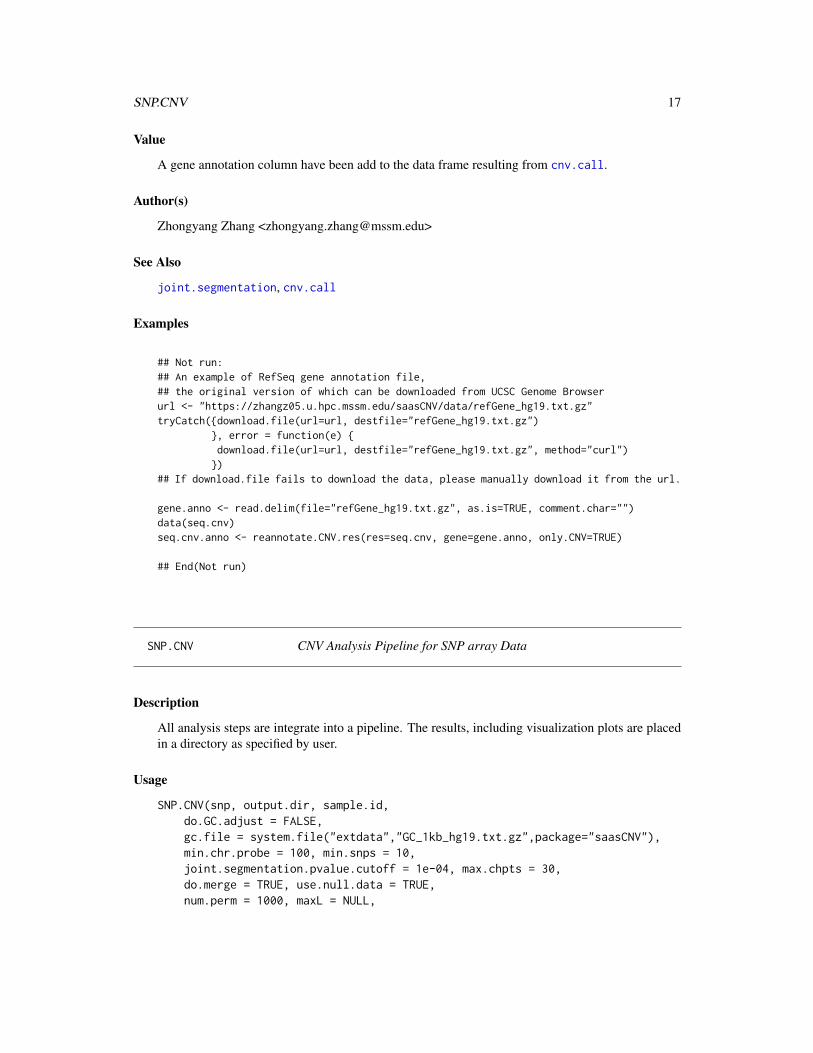
SNP.CNV CNV Analysis Pipeline for SNP array Data

Description

All analysis steps are integrate into a pipeline. The results, including visualization plots are placedin a directory as specified by user.

Usage

SNP.CNV(snp, output.dir, sample.id,do.GC.adjust = FALSE,gc.file = system.file("extdata","GC_1kb_hg19.txt.gz",package="saasCNV"),min.chr.probe = 100, min.snps = 10,joint.segmentation.pvalue.cutoff = 1e-04, max.chpts = 30,do.merge = TRUE, use.null.data = TRUE,num.perm = 1000, maxL = NULL,

18 SNP.CNV

merge.pvalue.cutoff = 0.05,do.cnvcall.on.merge = TRUE,cnvcall.pvalue.cutoff = 0.05,do.boundary.refine = FALSE,do.plot = TRUE, cex = 0.3,ref.num.probe = NULL,do.gene.anno = FALSE,gene.anno.file = NULL,seed = NULL, verbose = TRUE)

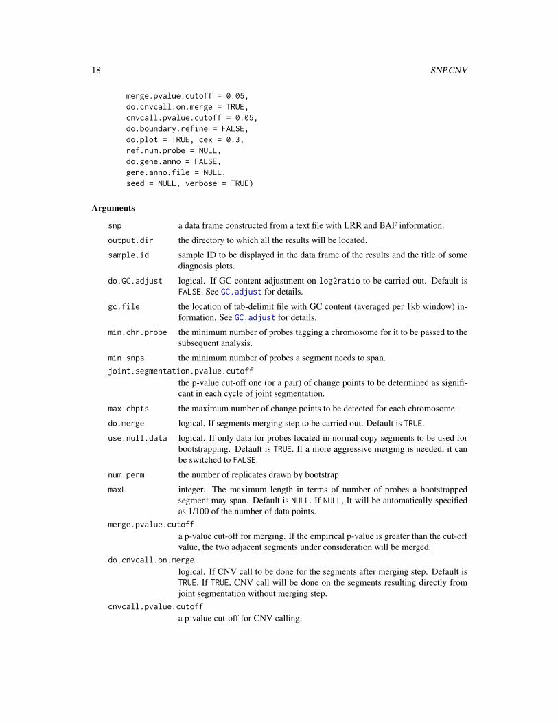
Arguments

snp a data frame constructed from a text file with LRR and BAF information.

output.dir the directory to which all the results will be located.

sample.id sample ID to be displayed in the data frame of the results and the title of somediagnosis plots.

do.GC.adjust logical. If GC content adjustment on log2ratio to be carried out. Default isFALSE. See GC.adjust for details.

gc.file the location of tab-delimit file with GC content (averaged per 1kb window) in-formation. See GC.adjust for details.


min.snps the minimum number of probes a segment needs to span.joint.segmentation.pvalue.cutoff

the p-value cut-off one (or a pair) of change points to be determined as signifi-cant in each cycle of joint segmentation.


do.merge logical. If segments merging step to be carried out. Default is TRUE.


num.perm the number of replicates drawn by bootstrap.


merge.pvalue.cutoff


do.cnvcall.on.merge

logical. If CNV call to be done for the segments after merging step. Default isTRUE. If TRUE, CNV call will be done on the segments resulting directly fromjoint segmentation without merging step.

cnvcall.pvalue.cutoff

a p-value cut-off for CNV calling.

SNP.CNV 19

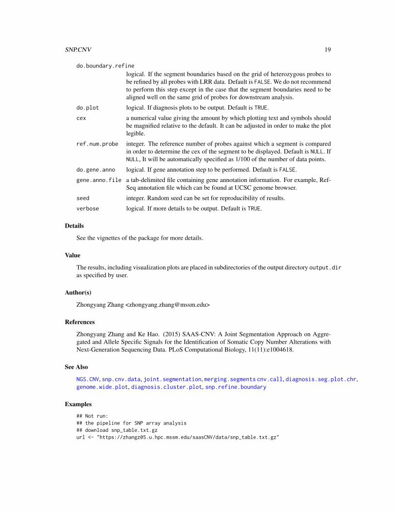
do.boundary.refine

logical. If the segment boundaries based on the grid of heterozygous probes tobe refined by all probes with LRR data. Default is FALSE. We do not recommendto perform this step except in the case that the segment boundaries need to bealigned well on the same grid of probes for downstream analysis.

do.plot logical. If diagnosis plots to be output. Default is TRUE.



do.gene.anno logical. If gene annotation step to be performed. Default is FALSE.

gene.anno.file a tab-delimited file containing gene annotation information. For example, Ref-Seq annotation file which can be found at UCSC genome browser.



Details


Value

The results, including visualization plots are placed in subdirectories of the output directory output.diras specified by user.

Author(s)


References

Zhongyang Zhang and Ke Hao. (2015) SAAS-CNV: A Joint Segmentation Approach on Aggre-gated and Allele Specific Signals for the Identification of Somatic Copy Number Alterations withNext-Generation Sequencing Data. PLoS Computational Biology, 11(11):e1004618.

See Also

NGS.CNV, snp.cnv.data, joint.segmentation, merging.segments cnv.call, diagnosis.seg.plot.chr,genome.wide.plot, diagnosis.cluster.plot, snp.refine.boundary

Examples

## Not run:## the pipeline for SNP array analysis## download snp_table.txt.gzurl <- "https://zhangz05.u.hpc.mssm.edu/saasCNV/data/snp_table.txt.gz"

20 snp.cnv.data

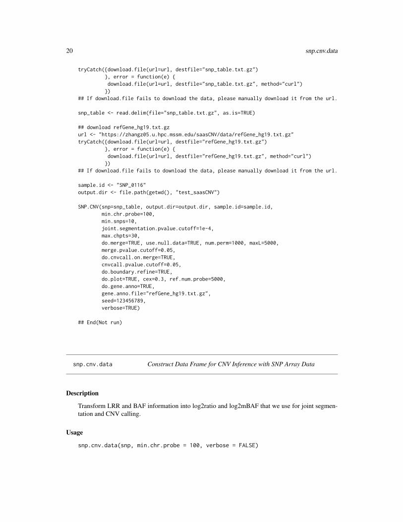
tryCatch({download.file(url=url, destfile="snp_table.txt.gz")}, error = function(e) {download.file(url=url, destfile="snp_table.txt.gz", method="curl")})


snp_table <- read.delim(file="snp_table.txt.gz", as.is=TRUE)

## download refGene_hg19.txt.gzurl <- "https://zhangz05.u.hpc.mssm.edu/saasCNV/data/refGene_hg19.txt.gz"tryCatch({download.file(url=url, destfile="refGene_hg19.txt.gz")



sample.id <- "SNP_0116"output.dir <- file.path(getwd(), "test_saasCNV")

SNP.CNV(snp=snp_table, output.dir=output.dir, sample.id=sample.id,min.chr.probe=100,min.snps=10,joint.segmentation.pvalue.cutoff=1e-4,max.chpts=30,do.merge=TRUE, use.null.data=TRUE, num.perm=1000, maxL=5000,merge.pvalue.cutoff=0.05,do.cnvcall.on.merge=TRUE,cnvcall.pvalue.cutoff=0.05,do.boundary.refine=TRUE,do.plot=TRUE, cex=0.3, ref.num.probe=5000,do.gene.anno=TRUE,gene.anno.file="refGene_hg19.txt.gz",seed=123456789,verbose=TRUE)

## End(Not run)

snp.cnv.data Construct Data Frame for CNV Inference with SNP Array Data

Description

Transform LRR and BAF information into log2ratio and log2mBAF that we use for joint segmen-tation and CNV calling.

Usage

snp.cnv.data(snp, min.chr.probe = 100, verbose = FALSE)

snp.cnv.data 21

Arguments

snp a data frame with LRR and BAF information from SNP array. See the examplebelow for details.


verbose logical. If more details to be output. Default is FALSE.

Value

A data frame containing the log2raio and log2mBAF values for each probe site.

Author(s)


References

Staaf, J., Vallon-Christersson, J., Lindgren, D., Juliusson, G., Rosenquist, R., Hoglund, M., Borg,A., Ringner, M. (2008) Normalization of Illumina Infinium whole-genome SNP data improves copynumber estimates and allelic intensity ratios. BMC bioinformatics, 9:409.

See Also

cnv.data

Examples

## Not run:## an example data with LRR and BAF informationurl <- "https://zhangz05.u.hpc.mssm.edu/saasCNV/data/snp_table.txt.gz"tryCatch({download.file(url=url, destfile="snp_table.txt.gz")

}, error = function(e) {download.file(url=url, destfile="snp_table.txt.gz", method="curl")})


snp_table <- read.delim(file="snp_table.txt.gz", as.is=TRUE)snp.data <- snp.cnv.data(snp=snp_table, min.chr.probe=100, verbose=TRUE)

## see how seq.data looks likeurl <- "https://zhangz05.u.hpc.mssm.edu/saasCNV/data/snp.data.RData"tryCatch({download.file(url=url, destfile="snp.data.RData")

}, error = function(e) {download.file(url=url, destfile="snp.data.RData", method="curl")})


load("snp.data.RData")head(snp.data)

22 snp.refine.boundary

## End(Not run)

snp.refine.boundary Refine Segment Boundaries

Description

Refine the segment boundaries based on the grid of heterozygous probes by all probes with LRRdata. We do not recommend to perform this step except in the case that the segment boundariesneed to be aligned well on the same grid of probes for downstream analysis.

Usage

snp.refine.boundary(data, segs.stat)

Arguments

data a data frame containing log2ratio and log2mBAF data generated by snp.cnv.data.

segs.stat a data frame containing segment locations and summary statistics resulting fromcnv.call.

Value

A data frame with the same columns as the one generated by cnv.call with the columns posStart,posEnd, length, chrIdxStart, chrIdxEnd and numProbe updated accordingly.

Author(s)


See Also

snp.cnv.data, cnv.call

Examples

## Not run:## download snp.data.RDataurl <- "https://zhangz05.u.hpc.mssm.edu/saasCNV/data/snp.data.RData"tryCatch({download.file(url=url, destfile="snp.data.RData")

}, error = function(e) {download.file(url=url, destfile="snp.data.RData", method="curl")})


load("snp.data.RData")data(snp.cnv)snp.cnv.refine <- snp.refine.boundary(data=snp.data, segs.stat=snp.cnv)

vcf2txt 23

## End(Not run)

## how the results look likedata(snp.cnv.refine)head(snp.cnv.refine)

vcf2txt Covert VCF File to A Data Frame

Description

It parses a VCF file and extract necessary information for CNV analysis.

Usage

vcf2txt(vcf.file, normal.col = 10, tumor.col = 11, MQ.cutoff = 30)

Arguments

vcf.file vcf file name.

normal.col the number of the column in which the genotype and read depth information ofnormal tissue are located in the vcf file.

tumor.col the number of the column in which the genotype and read depth information oftumor tissue are located in the vcf file.

MQ.cutoff the minimum criterion of mapping quality.

Details

Note that the first 9 columns in vcf file are mandatory, followed by the information for called variantstarting from the 10th column.

Value

A data frame of detailed information about each variant, including chrosome position, reference andalternative alleles, genotype and read depth carrying reference and alternative alleles for normal andtumor respectively.

Author(s)


References

Danecek, P., Auton, A., Abecasis, G., Albers, C. A., Banks, E., DePristo, M. A., Handsaker, R.E., Lunter, G., Marth, G. T., Sherry, S. T., et al. (2011) The variant call format and VCFtools.Bioinformatics, 27:2156–2158.

http://www.1000genomes.org/node/101

24 vcf2txt

Examples

## Not run:## an example VCF file from WES## download WES_example.vcf.gzurl <- "https://zhangz05.u.hpc.mssm.edu/saasCNV/data/WES_example.vcf.gz"tryCatch({download.file(url=url, destfile="WES_example.vcf.gz")

}, error = function(e) {download.file(url=url, destfile="WES_example.vcf.gz", method="curl")})


## convert VCf file to a data framevcf_table <- vcf2txt(vcf.file="WES_example.vcf.gz", normal.col=9+1, tumor.col=9+2)

## see how vcf_table looks like## download vcf_table.txt.gzurl <- "https://zhangz05.u.hpc.mssm.edu/saasCNV/data/vcf_table.txt.gz"tryCatch({download.file(url=url, destfile="vcf_table.txt.gz")



vcf_table <- read.delim(file="vcf_table.txt.gz", as.is=TRUE)head(vcf_table)

## End(Not run)

Index

∗Topic CBSjoint.segmentation, 10

∗Topic CNV callcnv.call, 3

∗Topic CNVcnv.call, 3cnv.data, 4GC.adjust, 8NGS.CNV, 13reannotate.CNV.res, 16SNP.CNV, 17snp.cnv.data, 20snp.refine.boundary, 22

∗Topic GC contentGC.adjust, 8

∗Topic NGSNGS.CNV, 13

∗Topic SCNAdiagnosis.cluster.plot, 5genome.wide.plot, 9

∗Topic SNP arraySNP.CNV, 17snp.refine.boundary, 22

∗Topic VCFvcf2txt, 23

∗Topic annotationreannotate.CNV.res, 16

∗Topic clusterdiagnosis.cluster.plot, 5

∗Topic diagnosisdiagnosis.cluster.plot, 5diagnosis.seg.plot.chr, 7genome.wide.plot, 9

∗Topic genereannotate.CNV.res, 16

∗Topic joint segmentationjoint.segmentation, 10

∗Topic mergemerging.segments, 12

∗Topic pipelineNGS.CNV, 13SNP.CNV, 17

∗Topic segmentationdiagnosis.seg.plot.chr, 7joint.segmentation, 10merging.segments, 12

∗Topic vcfvcf2txt, 23

∗Topic visualizationdiagnosis.cluster.plot, 5genome.wide.plot, 9

BAF2mBAF (internals), 10

check.overlap (internals), 10cnv.call, 3, 6, 9, 10, 15–17, 19, 22cnv.data, 3, 4, 4, 7–9, 11–13, 15, 21cnv.data.chr (internals), 10compute.baseline (internals), 10compute.var (internals), 10computeBeta (internals), 10computeMoments (internals), 10computeTiltDirect (internals), 10ComputeZ.fromS.R (internals), 10computeZ.onechange (internals), 10computeZ.squarewave.sample (internals),

10

dchi (internals), 10delta.sd (internals), 10diagnosis.cluster.plot, 3, 5, 10, 12, 15, 19diagnosis.QQ.plot (internals), 10diagnosis.seg.plot.chr, 6, 7, 10, 15, 19

fcompute.max.Z (internals), 10fmscbs (internals), 10fscan.max (internals), 10

GC.adjust, 8, 14, 18genome.wide.plot, 6, 9, 15, 19

25

26 INDEX

getCutoffMultisampleWeightedChisq(internals), 10

impute.missing.data (internals), 10internals, 10

joint.segmentation, 3, 4, 6, 7, 10, 10, 12,13, 15, 17, 19

matrix.max (internals), 10merging.segments, 3, 4, 7, 12, 15, 19merging.segments.chr (internals), 10Mode (internals), 10mscbs.classify (internals), 10

NGS.CNV, 13, 19

pmarg.sumweightedchisq (internals), 10pvalueMultisampleWeightedChisq

(internals), 10

reannotate.CNV.res, 16

saasCNV (saasCNV-package), 2saasCNV-package, 2seg.summary (internals), 10seq.cnv (internals), 10seq.data (internals), 10seq.segs (internals), 10SNP.CNV, 17snp.cnv (internals), 10snp.cnv.data, 8, 9, 19, 20, 22snp.data (internals), 10snp.refine.boundary, 19, 22snp.segs (internals), 10snp_table (internals), 10

vcf2txt, 4, 5, 14, 15, 23vcf_table (internals), 10vu (internals), 10

Package ‘saasCNV’ - R · cnv.call 3 Examples ## See the vignettes of the package for examples....

Documents

Transcript of Package ‘saasCNV’ - R · cnv.call 3 Examples ## See the vignettes of the package for examples....