![Protocol template (Protocol) N N For Preview Only · For Preview Only [Intervention Protocol] Protocol template N N1 1Not specified Contact address: N N, Not specified. Editorial](https://static.fdocuments.net/doc/165x107/5ebeff74dd82597f242a9b81/protocol-template-protocol-n-n-for-preview-only-for-preview-only-intervention.jpg)
Package ‘rgeos’ · PDF filePackage ‘rgeos ’ October 31, 2017 ......
77
Package ‘rgeos’ October 31, 2017 Title Interface to Geometry Engine - Open Source ('GEOS') Version 0.3-26 Date 2017-10-30 Depends R (>= 3.3.0) Imports methods, sp (>= 1.1-0), utils, stats, graphics LinkingTo sp Suggests maptools (>= 0.8-5), testthat, XML, maps, rgdal LazyLoad yes Description Interface to Geometry Engine - Open Source ('GEOS') using the C 'API' for topology op- erations on geometries. The 'GEOS' library is external to the package, and, when in- stalling the package from source, must be correctly installed first. Windows and Mac In- tel OS X binaries are provided on 'CRAN'. License GPL (>= 2) URL https://r-forge.r-project.org/projects/rgeos/ http://trac.osgeo.org/geos/ SystemRequirements GEOS (>= 3.2.0); for building from source: GEOS from http://trac.osgeo.org/geos/; GEOS OSX frameworks built by William Kyngesburye at http://www.kyngchaos.com/ may be used for source installs on OSX. NeedsCompilation yes Author Roger Bivand [cre, aut], Colin Rundel [aut], Edzer Pebesma [ctb], Rainer Stuetz [ctb], Karl Ove Hufthammer [ctb] Maintainer Roger Bivand <[email protected]> Repository CRAN Date/Publication 2017-10-31 13:17:54 UTC 1
Transcript of Package ‘rgeos’ · PDF filePackage ‘rgeos ’ October 31, 2017 ......

Package ‘rgeos’October 31, 2017
Title Interface to Geometry Engine - Open Source ('GEOS')
Version 0.3-26
Date 2017-10-30
Depends R (>= 3.3.0)
Imports methods, sp (>= 1.1-0), utils, stats, graphics
LinkingTo sp
Suggests maptools (>= 0.8-5), testthat, XML, maps, rgdal
LazyLoad yes
Description Interface to Geometry Engine - Open Source ('GEOS') using the C 'API' for topology op-erations on geometries. The 'GEOS' library is external to the package, and, when in-stalling the package from source, must be correctly installed first. Windows and Mac In-tel OS X binaries are provided on 'CRAN'.
License GPL (>= 2)
URL https://r-forge.r-project.org/projects/rgeos/
http://trac.osgeo.org/geos/
SystemRequirements GEOS (>= 3.2.0); for building from source: GEOSfrom http://trac.osgeo.org/geos/; GEOS OSX frameworks built byWilliam Kyngesburye at http://www.kyngchaos.com/ may be usedfor source installs on OSX.
NeedsCompilation yes
Author Roger Bivand [cre, aut],Colin Rundel [aut],Edzer Pebesma [ctb],Rainer Stuetz [ctb],Karl Ove Hufthammer [ctb]
Maintainer Roger Bivand <[email protected]>
Repository CRAN
Date/Publication 2017-10-31 13:17:54 UTC
1

2 R topics documented:
R topics documented:gArea . . . . . . . . . . . . . . . . . . . . . . . . . . . . . . . . . . . . . . . . . . . . 3gBoundary . . . . . . . . . . . . . . . . . . . . . . . . . . . . . . . . . . . . . . . . . . 4gBuffer . . . . . . . . . . . . . . . . . . . . . . . . . . . . . . . . . . . . . . . . . . . 5gCentroid . . . . . . . . . . . . . . . . . . . . . . . . . . . . . . . . . . . . . . . . . . 7gContains . . . . . . . . . . . . . . . . . . . . . . . . . . . . . . . . . . . . . . . . . . 8gConvexHull . . . . . . . . . . . . . . . . . . . . . . . . . . . . . . . . . . . . . . . . 11gCrosses . . . . . . . . . . . . . . . . . . . . . . . . . . . . . . . . . . . . . . . . . . . 12gDelaunayTriangulation . . . . . . . . . . . . . . . . . . . . . . . . . . . . . . . . . . 13gDifference . . . . . . . . . . . . . . . . . . . . . . . . . . . . . . . . . . . . . . . . . 15gDistance . . . . . . . . . . . . . . . . . . . . . . . . . . . . . . . . . . . . . . . . . . 16gEnvelope . . . . . . . . . . . . . . . . . . . . . . . . . . . . . . . . . . . . . . . . . . 18gEquals . . . . . . . . . . . . . . . . . . . . . . . . . . . . . . . . . . . . . . . . . . . 19gInterpolate . . . . . . . . . . . . . . . . . . . . . . . . . . . . . . . . . . . . . . . . . 21gIntersection . . . . . . . . . . . . . . . . . . . . . . . . . . . . . . . . . . . . . . . . 22gIntersects . . . . . . . . . . . . . . . . . . . . . . . . . . . . . . . . . . . . . . . . . . 24gIsEmpty . . . . . . . . . . . . . . . . . . . . . . . . . . . . . . . . . . . . . . . . . . 26gIsRing . . . . . . . . . . . . . . . . . . . . . . . . . . . . . . . . . . . . . . . . . . . 28gIsSimple . . . . . . . . . . . . . . . . . . . . . . . . . . . . . . . . . . . . . . . . . . 29gIsValid . . . . . . . . . . . . . . . . . . . . . . . . . . . . . . . . . . . . . . . . . . . 30gLength . . . . . . . . . . . . . . . . . . . . . . . . . . . . . . . . . . . . . . . . . . . 32gNearestPoints . . . . . . . . . . . . . . . . . . . . . . . . . . . . . . . . . . . . . . . 33gNode . . . . . . . . . . . . . . . . . . . . . . . . . . . . . . . . . . . . . . . . . . . . 34gpc.poly-class . . . . . . . . . . . . . . . . . . . . . . . . . . . . . . . . . . . . . . . . 35gpc.poly.nohole-class . . . . . . . . . . . . . . . . . . . . . . . . . . . . . . . . . . . . 38gPointOnSurface . . . . . . . . . . . . . . . . . . . . . . . . . . . . . . . . . . . . . . 39gPolygonize . . . . . . . . . . . . . . . . . . . . . . . . . . . . . . . . . . . . . . . . . 40gProject . . . . . . . . . . . . . . . . . . . . . . . . . . . . . . . . . . . . . . . . . . . 42gRelate . . . . . . . . . . . . . . . . . . . . . . . . . . . . . . . . . . . . . . . . . . . 43gSimplify . . . . . . . . . . . . . . . . . . . . . . . . . . . . . . . . . . . . . . . . . . 45gSymdifference . . . . . . . . . . . . . . . . . . . . . . . . . . . . . . . . . . . . . . . 46gTouches . . . . . . . . . . . . . . . . . . . . . . . . . . . . . . . . . . . . . . . . . . 48gUnion . . . . . . . . . . . . . . . . . . . . . . . . . . . . . . . . . . . . . . . . . . . 49new-generics . . . . . . . . . . . . . . . . . . . . . . . . . . . . . . . . . . . . . . . . 51over . . . . . . . . . . . . . . . . . . . . . . . . . . . . . . . . . . . . . . . . . . . . . 53polyfile . . . . . . . . . . . . . . . . . . . . . . . . . . . . . . . . . . . . . . . . . . . 54polygonsLabel . . . . . . . . . . . . . . . . . . . . . . . . . . . . . . . . . . . . . . . . 56RGEOS Experimental Functions . . . . . . . . . . . . . . . . . . . . . . . . . . . . . . 59RGEOS Polygon Hole Comment Functions . . . . . . . . . . . . . . . . . . . . . . . . 60RGEOS Utility Functions . . . . . . . . . . . . . . . . . . . . . . . . . . . . . . . . . . 63RGEOS WKT Functions . . . . . . . . . . . . . . . . . . . . . . . . . . . . . . . . . . 66Ring-class . . . . . . . . . . . . . . . . . . . . . . . . . . . . . . . . . . . . . . . . . . 67SpatialCollections . . . . . . . . . . . . . . . . . . . . . . . . . . . . . . . . . . . . . . 68SpatialCollections-class . . . . . . . . . . . . . . . . . . . . . . . . . . . . . . . . . . . 69SpatialRings . . . . . . . . . . . . . . . . . . . . . . . . . . . . . . . . . . . . . . . . . 70SpatialRings-class . . . . . . . . . . . . . . . . . . . . . . . . . . . . . . . . . . . . . . 71SpatialRingsDataFrame-class . . . . . . . . . . . . . . . . . . . . . . . . . . . . . . . . 72

gArea 3
Index 74
gArea Area of Geometry
Description
Calculates the area of the given geometry.
Usage
gArea(spgeom, byid=FALSE)
Arguments
spgeom sp object as defined in package sp
byid Logical determining if the function should be applied across subgeometries(TRUE) or the entire object (FALSE)
Value
Returns the area of the geometry in the units of the current projection. By definition non-[MULTI]POLYGONgeometries have an area of 0. The area of a POLYGON is the area of its shell less the area of anyholes. Note that this value may be different from the area slot of the Polygons class as this valuedoes not subtract the area of any holes in the geometry.
Author(s)
Roger Bivand & Colin Rundel
See Also
gLength
Examples
gArea(readWKT("POINT(1 1)"))gArea(readWKT("LINESTRING(0 0,1 1,2 2)"))gArea(readWKT("LINEARRING(0 0,3 0,3 3,0 3,0 0)"))
p1 = readWKT("POLYGON((0 0,3 0,3 3,0 3,0 0))")p2 = readWKT("POLYGON((0 0,3 0,3 3,0 3,0 0),(1 1,2 1,2 2,1 2,1 1))")
gArea(p1)p1@polygons[[1]]@area
gArea(p2)p2@polygons[[1]]@area

4 gBoundary
gBoundary Boundary of Geometry
Description
Function for determinging the Boundary of the given geometry as defined by SFS Section 2.1.13.1
Usage
gBoundary(spgeom, byid=FALSE, id = NULL)
Arguments
spgeom sp object as defined in package sp
byid Logical determining if the function should be applied across subgeometries(TRUE) or the entire object (FALSE)
id Character vector defining id labels for the resulting geometries, if unspecifiedreturned geometries will be labeled based on their parent geometries’ labels.
Value
Depending of the class of the spgeom the returned results will differ.
Based on the documentation of JTS (on which GEOS is based) the following outputs are expected:
Point empty GeometryCollectionMultiPoint empty GeometryCollectionLineString if closed: empty MultiPoint if not closed: MultiPoint containing the two endpoints.MultiLineString MultiPoint obtained by applying the Mod-2 rule to the boundaries of the element LineStringsLinearRing empty MultiPointPolygon MultiLineString containing the LinearRings of the shell and holes, in that order (SFS 2.1.10)MultiPolygon MultiLineString containing the LinearRings for the boundaries of the element polygons, in the same order as they occur in the MultiPolygon (SFS 2.1.12/JTS)GeometryCollection The boundary of an arbitrary collection of geometries whose interiors are disjoint consist of geometries drawn from the boundaries of the element geometries by application of the Mod-2 rule (SFS Section 2.1.13.1)
The mod-2 rule states that for a multiline a point is on the boundary if and only if it on the boundaryof an odd number of subgeometries of the multiline (See example below).
Author(s)
Roger Bivand & Colin Rundel
See Also
gCentroid gConvexHull gEnvelope gPointOnSurface

gBuffer 5
Examples
x = readWKT("POLYGON((0 0,10 0,10 10,0 10,0 0))")b = gBoundary(x)
plot(x,col='black')plot(b,col='red',lwd=3,add=TRUE)
# mod-2 rule examplex1 = readWKT("MULTILINESTRING((2 2,2 0),(2 2,0 2))")x2 = readWKT("MULTILINESTRING((2 2,2 0),(2 2,0 2),(2 2,4 2))")x3 = readWKT("MULTILINESTRING((2 2,2 0),(2 2,0 2),(2 2,4 2),(2 2,2 4))")x4 = readWKT("MULTILINESTRING((2 2,2 0),(2 2,0 2),(2 2,4 2),(2 2,2 4),(2 2,4 4))")
b1 = gBoundary(x1)b2 = gBoundary(x2)b3 = gBoundary(x3)b4 = gBoundary(x4)
par(mfrow=c(2,2))plot(x1); plot(b1,pch=16,col='red',add=TRUE)plot(x2); plot(b2,pch=16,col='red',add=TRUE)plot(x3); plot(b3,pch=16,col='red',add=TRUE)plot(x4); plot(b4,pch=16,col='red',add=TRUE)
gBuffer Buffer Geometry
Description
Expands the given geometry to include the area within the specified width with specific stylingoptions.
Usage
gBuffer(spgeom, byid=FALSE, id=NULL, width=1.0, quadsegs=5, capStyle="ROUND",joinStyle="ROUND", mitreLimit=1.0)
Arguments
spgeom sp object as defined in package sp
byid Logical determining if the function should be applied across subgeometries(TRUE) or the entire object (FALSE)
id Character vector defining id labels for the resulting geometries, if unspecifiedreturned geometries will be labeled based on their parent geometries’ labels.

6 gBuffer
width Distance from original geometry to include in the new geometry. Negative val-ues are allowed. Either a numeric vector of length 1 when byid is FALSE; ifbyid is TRUE: of length 1 replicated to the number of input geometries, or oflength equal to the number of input geometries
quadsegs Number of line segments to use to approximate a quarter circle.
capStyle Style of cap to use at the ends of the geometry. Allowed values: ROUND,FLAT,SQUARE
joinStyle Style to use for joints in the geometry. Allowed values: ROUND,MITRE,BEVEL
mitreLimit Numerical value that specifies how far a joint can extend if a mitre join style isused.
Value
SpatialPolygons (or a SpatialPolygonsDataFrame if byid=TRUE and spgeom has a data.frame); ifnegative width(s) lead the object to disappear, NULL is returned for byid FALSE, and componentPolygons objects are dropped if empty for byid TRUE; the SpatialPolygonsDataFrame is subsettedby row.names or id if given to retain non-empty geometry rows
Author(s)
Roger Bivand & Colin Rundel
Examples
p1 = readWKT("POLYGON((0 1,0.95 0.31,0.59 -0.81,-0.59 -0.81,-0.95 0.31,0 1))")p2 = readWKT("POLYGON((2 2,-2 2,-2 -2,2 -2,2 2),(1 1,-1 1,-1 -1,1 -1,1 1))")
par(mfrow=c(2,3))plot(gBuffer(p1,width=-0.2),col='black',xlim=c(-1.5,1.5),ylim=c(-1.5,1.5))plot(p1,border='blue',lwd=2,add=TRUE);title("width: -0.2")plot(gBuffer(p1,width=0),col='black',xlim=c(-1.5,1.5),ylim=c(-1.5,1.5))plot(p1,border='blue',lwd=2,add=TRUE);title("width: 0")plot(gBuffer(p1,width=0.2),col='black',xlim=c(-1.5,1.5),ylim=c(-1.5,1.5))plot(p1,border='blue',lwd=2,add=TRUE);title("width: 0.2")
plot(gBuffer(p2,width=-0.2),col='black',pbg='white',xlim=c(-2.5,2.5),ylim=c(-2.5,2.5))plot(p2,border='blue',lwd=2,add=TRUE);title("width: -0.2")plot(gBuffer(p2,width=0),col='black',pbg='white',xlim=c(-2.5,2.5),ylim=c(-2.5,2.5))plot(p2,border='blue',lwd=2,add=TRUE);title("width: 0")plot(gBuffer(p2,width=0.2),col='black',pbg='white',xlim=c(-2.5,2.5),ylim=c(-2.5,2.5))plot(p2,border='blue',lwd=2,add=TRUE);title("width: 0.2")
p3 <- readWKT(paste("GEOMETRYCOLLECTION(","POLYGON((0 1,0.95 0.31,0.59 -0.81,-0.59 -0.81,-0.95 0.31,0 1)),","POLYGON((2 2,-2 2,-2 -2,2 -2,2 2),(1 1,-1 1,-1 -1,1 -1,1 1)))"))
par(mfrow=c(1,1))plot(gBuffer(p3, byid=TRUE, width=c(-0.2, -0.1)),col='black',pbg='white',xlim=c(-2.5,2.5),ylim=c(-2.5,2.5))plot(p3,border=c('blue', 'red'),lwd=2,add=TRUE);title("width: -0.2, -0.1")
gCentroid 7
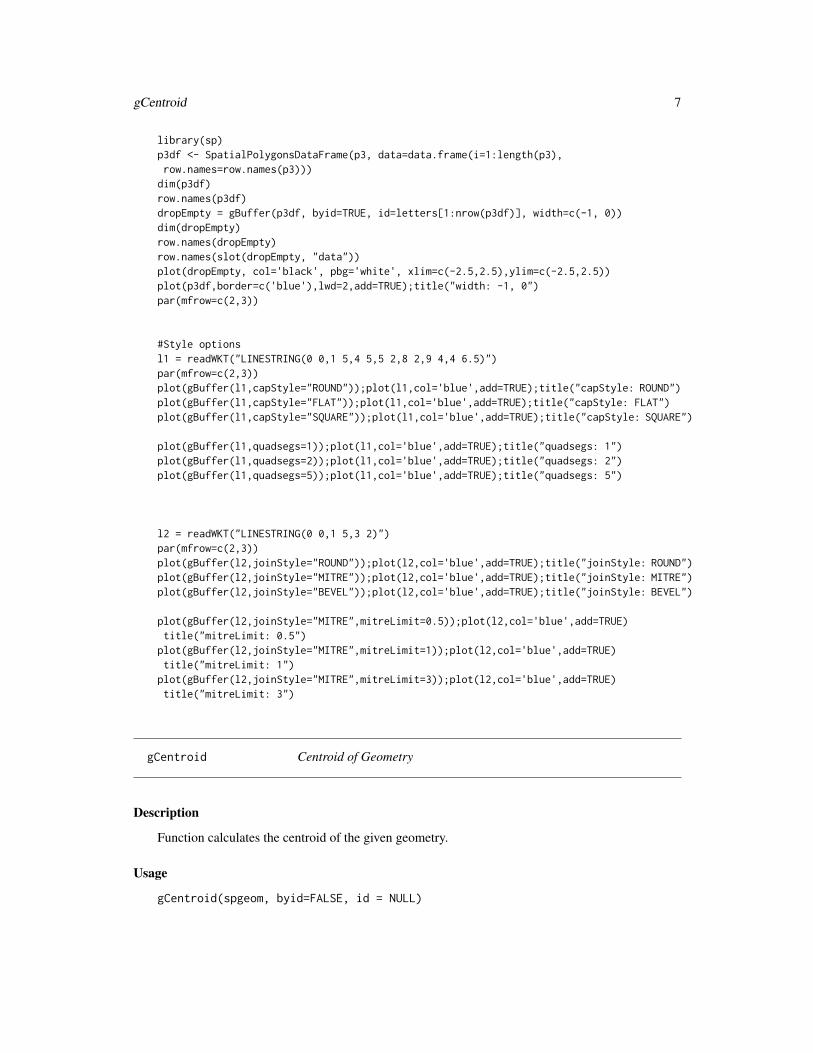
library(sp)p3df <- SpatialPolygonsDataFrame(p3, data=data.frame(i=1:length(p3),row.names=row.names(p3)))
dim(p3df)row.names(p3df)dropEmpty = gBuffer(p3df, byid=TRUE, id=letters[1:nrow(p3df)], width=c(-1, 0))dim(dropEmpty)row.names(dropEmpty)row.names(slot(dropEmpty, "data"))plot(dropEmpty, col='black', pbg='white', xlim=c(-2.5,2.5),ylim=c(-2.5,2.5))plot(p3df,border=c('blue'),lwd=2,add=TRUE);title("width: -1, 0")par(mfrow=c(2,3))
#Style optionsl1 = readWKT("LINESTRING(0 0,1 5,4 5,5 2,8 2,9 4,4 6.5)")par(mfrow=c(2,3))plot(gBuffer(l1,capStyle="ROUND"));plot(l1,col='blue',add=TRUE);title("capStyle: ROUND")plot(gBuffer(l1,capStyle="FLAT"));plot(l1,col='blue',add=TRUE);title("capStyle: FLAT")plot(gBuffer(l1,capStyle="SQUARE"));plot(l1,col='blue',add=TRUE);title("capStyle: SQUARE")
plot(gBuffer(l1,quadsegs=1));plot(l1,col='blue',add=TRUE);title("quadsegs: 1")plot(gBuffer(l1,quadsegs=2));plot(l1,col='blue',add=TRUE);title("quadsegs: 2")plot(gBuffer(l1,quadsegs=5));plot(l1,col='blue',add=TRUE);title("quadsegs: 5")
l2 = readWKT("LINESTRING(0 0,1 5,3 2)")par(mfrow=c(2,3))plot(gBuffer(l2,joinStyle="ROUND"));plot(l2,col='blue',add=TRUE);title("joinStyle: ROUND")plot(gBuffer(l2,joinStyle="MITRE"));plot(l2,col='blue',add=TRUE);title("joinStyle: MITRE")plot(gBuffer(l2,joinStyle="BEVEL"));plot(l2,col='blue',add=TRUE);title("joinStyle: BEVEL")
plot(gBuffer(l2,joinStyle="MITRE",mitreLimit=0.5));plot(l2,col='blue',add=TRUE)title("mitreLimit: 0.5")plot(gBuffer(l2,joinStyle="MITRE",mitreLimit=1));plot(l2,col='blue',add=TRUE)title("mitreLimit: 1")plot(gBuffer(l2,joinStyle="MITRE",mitreLimit=3));plot(l2,col='blue',add=TRUE)title("mitreLimit: 3")
gCentroid Centroid of Geometry
Description
Function calculates the centroid of the given geometry.
Usage
gCentroid(spgeom, byid=FALSE, id = NULL)

8 gContains
Arguments
spgeom sp object as defined in package sp
byid Logical determining if the function should be applied across subgeometries(TRUE) or the entire object (FALSE)
id Character vector defining id labels for the resulting geometries, if unspecifiedreturned geometries will be labeled based on their parent geometries’ labels.
Details
Returns a SpatialPoints object of the centroid(s) for spgeom.
Author(s)
Roger Bivand & Colin Rundel
See Also
gBoundary gConvexHull gEnvelope gPointOnSurface
Examples
x = readWKT(paste("GEOMETRYCOLLECTION(POLYGON((0 0,10 0,10 10,0 10,0 0)),","POLYGON((15 0,25 15,35 0,15 0)))"))
# Centroids of both the square and circle independentlyc1 = gCentroid(x,byid=TRUE)# Centroid of square and circle togetherc2 = gCentroid(x)
plot(x)plot(c1,col='red',add=TRUE)plot(c2,col='blue',add=TRUE)
gContains Geometry Relationships - Contains and Within
Description
Functions for testing whether one geometry contains or is contained within another geometry

gContains 9
Usage
gContains(spgeom1, spgeom2 = NULL, byid = FALSE, prepared=TRUE,returnDense=TRUE, STRsubset=FALSE, checkValidity=FALSE)
gContainsProperly(spgeom1, spgeom2 = NULL, byid = FALSE, returnDense=TRUE,checkValidity=FALSE)
gCovers(spgeom1, spgeom2 = NULL, byid = FALSE, returnDense=TRUE, checkValidity=FALSE)gCoveredBy(spgeom1, spgeom2 = NULL, byid = FALSE, returnDense=TRUE, checkValidity=FALSE)gWithin(spgeom1, spgeom2 = NULL, byid = FALSE, returnDense=TRUE, checkValidity=FALSE)
Argumentsspgeom1, spgeom2
sp objects as defined in package sp. If spgeom2 is NULL then spgeom1 iscompared to itself.
byid Logical vector determining if the function should be applied across ids (TRUE)or the entire object (FALSE) for spgeom1 and spgeom2
prepared Logical determining if prepared geometry (spatially indexed) version of theGEOS function should be used. In general prepared geometries should be fasterthan the alternative.
returnDense default TRUE, if false returns a list of the length of spgeom1 of integer vec-tors listing the 1:length(spgeom2) indices which would be TRUE in the denselogical matrix representation; useful when the sizes of the byid=TRUE returnedmatrix is very large and it is sparse; essential when the returned matrix wouldbe too large
checkValidity default FALSE; error meesages from GEOS do not say clearly which object failsif a topology exception is encountered. If this argument is TRUE, gIsValid isrun on each in turn in an environment in which object names are available. Ifobjects are invalid, this is reported and those affected are named
STRsubset logical argument for future use
Value
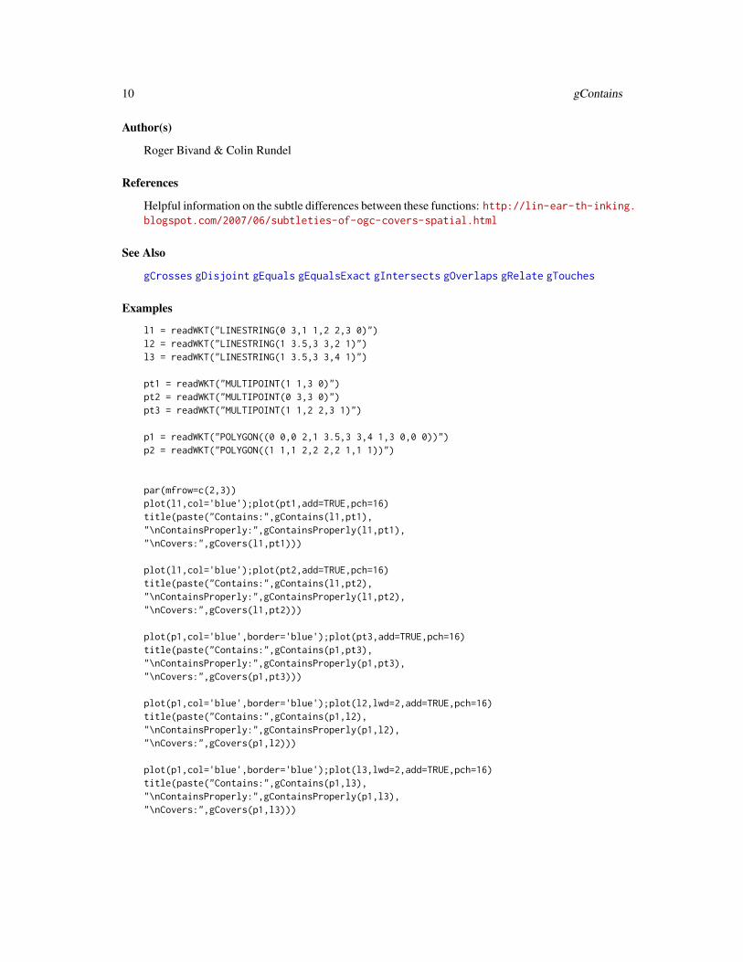
gContains returns TRUE if none of the point of spgeom2 is outside of spgeom1 and at least onepoint of spgeom2 falls within spgeom1.
gContainsProperly returns TRUE under the same conditions as gContains with the additionalrequirement that spgeom2 does not intersect with the boundary of spgeom1. As such any givengeometry will Contain itself but will not ContainProperly itself.
gCovers returns TRUE if no point in spgeom2 is outside of spgeom1. This is slightly different fromgContains as it does not require a point within spgeom1 which can be an issue as boundaries arenot considered to be "within" a geometry, see gBoundary for specifics of geometry boundaries.
gCoveredBy is the converse of gCovers and is equivalent to swapping spgeom1 and spgeom2.
gWithin is the converse of gContains and is equivalent to swapping spgeom1 and spgeom2.
Note
Error messages from GEOS, in particular topology exceptions, report 0-based object order, so geom0 is spgeom1, and geom 1 is spgeom2.
10 gContains
Author(s)
Roger Bivand & Colin Rundel
References
Helpful information on the subtle differences between these functions: http://lin-ear-th-inking.blogspot.com/2007/06/subtleties-of-ogc-covers-spatial.html
See Also
gCrosses gDisjoint gEquals gEqualsExact gIntersects gOverlaps gRelate gTouches
Examples
l1 = readWKT("LINESTRING(0 3,1 1,2 2,3 0)")l2 = readWKT("LINESTRING(1 3.5,3 3,2 1)")l3 = readWKT("LINESTRING(1 3.5,3 3,4 1)")
pt1 = readWKT("MULTIPOINT(1 1,3 0)")pt2 = readWKT("MULTIPOINT(0 3,3 0)")pt3 = readWKT("MULTIPOINT(1 1,2 2,3 1)")
p1 = readWKT("POLYGON((0 0,0 2,1 3.5,3 3,4 1,3 0,0 0))")p2 = readWKT("POLYGON((1 1,1 2,2 2,2 1,1 1))")
par(mfrow=c(2,3))plot(l1,col='blue');plot(pt1,add=TRUE,pch=16)title(paste("Contains:",gContains(l1,pt1),"\nContainsProperly:",gContainsProperly(l1,pt1),"\nCovers:",gCovers(l1,pt1)))
plot(l1,col='blue');plot(pt2,add=TRUE,pch=16)title(paste("Contains:",gContains(l1,pt2),"\nContainsProperly:",gContainsProperly(l1,pt2),"\nCovers:",gCovers(l1,pt2)))
plot(p1,col='blue',border='blue');plot(pt3,add=TRUE,pch=16)title(paste("Contains:",gContains(p1,pt3),"\nContainsProperly:",gContainsProperly(p1,pt3),"\nCovers:",gCovers(p1,pt3)))
plot(p1,col='blue',border='blue');plot(l2,lwd=2,add=TRUE,pch=16)title(paste("Contains:",gContains(p1,l2),"\nContainsProperly:",gContainsProperly(p1,l2),"\nCovers:",gCovers(p1,l2)))
plot(p1,col='blue',border='blue');plot(l3,lwd=2,add=TRUE,pch=16)title(paste("Contains:",gContains(p1,l3),"\nContainsProperly:",gContainsProperly(p1,l3),"\nCovers:",gCovers(p1,l3)))

gConvexHull 11
plot(p1,col='blue',border='blue');plot(p2,col='black',add=TRUE,pch=16)title(paste("Contains:",gContains(p1,p2),"\nContainsProperly:",gContainsProperly(p1,p2),"\nCovers:",gCovers(p1,p2)))
gConvexHull Convex Hull of Geometry
Description
Function produces the Convex Hull of the given geometry, the smallest convex polygon that containsall subgeometries
Usage
gConvexHull(spgeom, byid=FALSE, id = NULL)
Arguments
spgeom sp object as defined in package sp
byid Logical determining if the function should be applied across subgeometries(TRUE) or the entire object (FALSE)
id Character vector defining id labels for the resulting geometries, if unspecifiedreturned geometries will be labeled based on their parent geometries’ labels.
Details
Returns the convex hull as a SpatialPolygons object.
Author(s)
Roger Bivand & Colin Rundel
See Also
gBoundary gCentroid gEnvelope gPointOnSurface
Examples
x = readWKT(paste("POLYGON((0 40,10 50,0 60,40 60,40 100,50 90,60 100,60","60,100 60,90 50,100 40,60 40,60 0,50 10,40 0,40 40,0 40))"))
ch = gConvexHull(x)
plot(x,col='blue',border='blue')plot(ch,add=TRUE)

12 gCrosses
gCrosses Geometry Relationships - Crosses and Overlaps
Description
Functions for testing whether geometries share some but not all interior points
Usage
gCrosses(spgeom1, spgeom2 = NULL, byid = FALSE, returnDense=TRUE,checkValidity=FALSE)
gOverlaps(spgeom1, spgeom2 = NULL, byid = FALSE, returnDense=TRUE,checkValidity=FALSE)
Argumentsspgeom1, spgeom2
sp objects as defined in package sp. If spgeom2 is NULL then spgeom1 iscompared to itself.
byid Logical vector determining if the function should be applied across ids (TRUE)or the entire object (FALSE) for spgeom1 and spgeom2
returnDense default TRUE, if false returns a list of the length of spgeom1 of integer vec-tors listing the 1:length(spgeom2) indices which would be TRUE in the denselogical matrix representation; useful when the sizes of the byid=TRUE returnedmatrix is very large and it is sparse; essential when the returned matrix wouldbe too large
checkValidity default FALSE; error meesages from GEOS do not say clearly which object failsif a topology exception is encountered. If this argument is TRUE, gIsValid isrun on each in turn in an environment in which object names are available. Ifobjects are invalid, this is reported and those affected are named
Value
gCrosses returns TRUE when the geometries share some but not all interior points, and the dimen-sion of the intersection is less than that of at least one of the geometries.
gOverlaps returns TRUE when the geometries share some but not all interior points, and the inter-section has the same dimension as the geometries themselves.
Note
Error messages from GEOS, in particular topology exceptions, report 0-based object order, so geom0 is spgeom1, and geom 1 is spgeom2.
Author(s)
Roger Bivand & Colin Rundel

gDelaunayTriangulation 13
See Also
gContains gContainsProperly gCovers gCoveredBy gDisjoint gEquals gEqualsExact gIntersectsgRelate gTouches gWithin
Examples
l1 = readWKT("LINESTRING(0 3,1 1,2 2,3 0)")l2 = readWKT("LINESTRING(0 0.5,1 1,2 2,3 2.5)")l3 = readWKT("LINESTRING(1 3,1.5 1,2.5 2)")
pt1 = readWKT("MULTIPOINT(1 1,3 0)")pt2 = readWKT("MULTIPOINT(1 1,3 0,1 2)")
p1 = readWKT("POLYGON((0 0,0 2,1 3.5,3 3,4 1,3 0,0 0))")p2 = readWKT("POLYGON((2 2,3 4,4 1,4 0,2 2))")
par(mfrow=c(2,3))plot(l1,col='blue');plot(pt1,add=TRUE,pch=16)title(paste("Crosses:",gCrosses(l1,pt1),"\nOverlaps:",gOverlaps(l1,pt1)))
plot(l1,col='blue');plot(pt2,add=TRUE,pch=16)title(paste("Crosses:",gCrosses(l1,pt2),"\nOverlaps:",gOverlaps(l1,pt2)))
plot(l1,col='blue');plot(l2,add=TRUE)title(paste("Crosses:",gCrosses(l1,l2),"\nOverlaps:",gOverlaps(l1,l2)))
plot(l1,col='blue');plot(l3,add=TRUE)title(paste("Crosses:",gCrosses(l1,l3),"\nOverlaps:",gOverlaps(l1,l3)))
plot(p1,border='blue',col='blue');plot(l1,add=TRUE)title(paste("Crosses:",gCrosses(p1,l1),"\nOverlaps:",gOverlaps(p1,l1)))
plot(p1,border='blue',col='blue');plot(p2,add=TRUE)title(paste("Crosses:",gCrosses(p1,p2),"\nOverlaps:",gOverlaps(p1,p2)))
gDelaunayTriangulation
Compute Delaunay triangulation between points
Description
Function to compute the Delaunay triangulation between points; only available for GEOS >= 3.4.0.

14 gDelaunayTriangulation
Usage
gDelaunayTriangulation(spgeom, tolerance=0.0, onlyEdges=FALSE)
Arguments
spgeom sp points object as defined in package sp
tolerance Numerical tolerance value to be used in triangulation
onlyEdges Logical, default returns triangles as polygons, if TRUE, returns a SpatialLinesobject with a single MULTILINESTRING
Details
When onlyEdges is TRUE, the SpatialLines object may be de-merged to identify the input pointsthat are touched by each edge, making it possible to identify spatial neighbours.
Value
Either a SpatialPolygons object or a SpatialLines object containing a single Lines object of theundirected edges in the triangulation.
Author(s)
Roger Bivand
References
http://en.wikipedia.org/wiki/Delaunay_triangulation
Examples
if (version_GEOS0() > "3.4.0") {library(sp)data(meuse)coordinates(meuse) <- c("x", "y")plot(gDelaunayTriangulation(meuse))points(meuse)out <- gDelaunayTriangulation(meuse, onlyEdges=TRUE)lns <- slot(slot(out, "lines")[[1]], "Lines")out1 <- SpatialLines(lapply(seq(along=lns), function(i) Lines(list(lns[[i]]),ID=as.character(i))))
out2 <- lapply(1:length(out1), function(i) which(gTouches(meuse, out1[i],byid=TRUE)))
out3 <- do.call("rbind", out2)o <- order(out3[,1], out3[,2])out4 <- out3[o,]out5 <- data.frame(from=out4[,1], to=out4[,2], weight=1)head(out5)## Not run:if (require(spdep)) {class(out5) <- c("spatial.neighbour", class(out5))

gDifference 15
attr(out5, "n") <- length(meuse)attr(out5, "region.id") <- as.character(1:length(meuse))nb1 <- sn2listw(out5)$neighboursnb2 <- make.sym.nb(nb1)}
## End(Not run)}
gDifference Geometry Difference
Description
Function for determining the difference between the two given geometries.
Usage
gDifference(spgeom1, spgeom2, byid=FALSE, id=NULL, drop_lower_td=FALSE,unaryUnion_if_byid_false=TRUE, checkValidity=FALSE)
Argumentsspgeom1, spgeom2
sp objects as defined in package sp
byid Logical vector determining if the function should be applied across ids (TRUE)or the entire object (FALSE) for spgeom1 and spgeom2
id Character vector defining id labels for the resulting geometries, if unspecifiedreturned geometries will be labeled based on their parent geometries’ labels.
drop_lower_td default FALSE; if TRUE, objects will be dropped from output GEOMETRYCOL-LECTION objects to simplify output if their topological dinension is less thanthe minimum topological dinension of the input objects.
unaryUnion_if_byid_false
default TRUE; if byid takes a FALSE in either position, the subgeometries arecombined first to avoid possible topology exceptions (change in 0.3-13, previousbehaviour did not combine subgeometries, and may be achieved by setting thisargument FALSE
checkValidity default FALSE; error meesages from GEOS do not say clearly which object failsif a topology exception is encountered. If this argument is TRUE, gIsValid isrun on each in turn in an environment in which object names are available. Ifobjects are invalid, this is reported and those affected are named
Details
Returns the regions of spgeom1 that are not within spgeom2. If the geometries do not intersect thenthe result is just spgeom1. Note that the function is not symmetric for spgeom1 and spgeom2.

16 gDistance
Note
Error messages from GEOS, in particular topology exceptions, report 0-based object order, so geom0 is spgeom1, and geom 1 is spgeom2.
Author(s)
Roger Bivand & Colin Rundel
See Also
gIntersection gSymdifference gUnion
Examples
x = readWKT("POLYGON ((0 0, 0 10, 10 10, 10 0, 0 0))")y = readWKT("POLYGON ((3 3, 7 3, 7 7, 3 7, 3 3))")
d = gDifference(x,y)plot(d,col='red',pbg='white')
# Empty geometry since y is completely contained with xd2 = gDifference(y,x)
gDistance Distance between geometries
Description
Calculates the distance between the given geometries
Usage
gDistance(spgeom1, spgeom2=NULL, byid=FALSE, hausdorff=FALSE, densifyFrac = NULL)gWithinDistance(spgeom1, spgeom2=NULL, dist, byid=FALSE,hausdorff=FALSE, densifyFrac=NULL)
Argumentsspgeom1, spgeom2
sp objects as defined in package sp. If spgeom2 is NULL then spgeom1 iscompared to itself.
byid Logical vector determining if the function should be applied across ids (TRUE)or the entire object (FALSE) for spgeom1 and spgeom2
hausdorff Logical determining if the discrete Hausdorff distance should be calculated
densifyFrac Numerical value between 0 and 1 that determines the fraction by which to den-sify each segment of the geometry.
dist Numerical value that determines cutoff distance

gDistance 17
Details
Discrete Hausdorff distance is essentially a measure of the similarity or dissimilarity of the twogeometries, see references below for more detailed explanations / descriptions.
If hausdorff is TRUE and densifyFrac is specified then the geometries’ segments are densifiedby splitting each segment into equal length subsegments whose fraction of the total length is equalto densifyFrac.
Value
gDistance by default returns the cartesian minimum distance between the two geometries in theunits of the current projection. If hausdorff is TRUE then the Hausdorff distance is returned forthe two geometries.
gWithinDistance returns TRUE if returned distance is less than or equal to the specified dist.
Author(s)
Roger Bivand & Colin Rundel
References
Hausdorff Differences: http://en.wikipedia.org/wiki/Hausdorff_distance http://lin-ear-th-inking.blogspot.com/2009/01/computing-geometric-similarity.html
See Also
gWithinDistance
Examples
pt1 = readWKT("POINT(0.5 0.5)")pt2 = readWKT("POINT(2 2)")
p1 = readWKT("POLYGON((0 0,1 0,1 1,0 1,0 0))")p2 = readWKT("POLYGON((2 0,3 1,4 0,2 0))")
gDistance(pt1,pt2)gDistance(p1,pt1)gDistance(p1,pt2)gDistance(p1,p2)
p3 = readWKT("POLYGON((0 0,2 0,2 2,0 2,0 0))")p4 = readWKT("POLYGON((0 0,2 0,2 1.9,1.9 2,0 2,0 0))")p5 = readWKT("POLYGON((0 0,2 0,2 1.5,1.5 2,0 2,0 0))")p6 = readWKT("POLYGON((0 0,2 0,2 1,1 2,0 2,0 0))")p7 = readWKT("POLYGON((0 0,2 0,0 2,0 0))")
gDistance(p3,hausdorff=TRUE)gDistance(p3,p4,hausdorff=TRUE)
18 gEnvelope
gDistance(p3,p5,hausdorff=TRUE)gDistance(p3,p6,hausdorff=TRUE)gDistance(p3,p7,hausdorff=TRUE)
gEnvelope Envelope of Geometry
Description
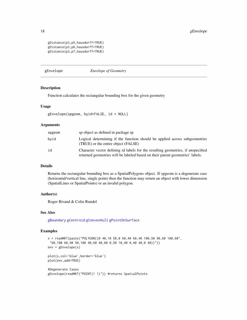
Function calculates the rectangular bounding box for the given geometry
Usage
gEnvelope(spgeom, byid=FALSE, id = NULL)
Arguments
spgeom sp object as defined in package sp
byid Logical determining if the function should be applied across subgeometries(TRUE) or the entire object (FALSE)
id Character vector defining id labels for the resulting geometries, if unspecifiedreturned geometries will be labeled based on their parent geometries’ labels.
Details
Returns the rectangular bounding box as a SpatialPolygons object. If spgeom is a degenerate case(horizontal/vertical line, single point) then the function may return an object with lower dimension(SpatialLines or SpatialPoints) or an invalid polygon.
Author(s)
Roger Bivand & Colin Rundel
See Also
gBoundary gCentroid gConvexHull gPointOnSurface
Examples
x = readWKT(paste("POLYGON((0 40,10 50,0 60,40 60,40 100,50 90,60 100,60","60,100 60,90 50,100 40,60 40,60 0,50 10,40 0,40 40,0 40))"))
env = gEnvelope(x)
plot(x,col='blue',border='blue')plot(env,add=TRUE)
#Degenerate CasesgEnvelope(readWKT("POINT(1 1)")) #returns SpatialPoints

gEquals 19
gEnvelope(readWKT("LINESTRING(1 1,1 2)")) #invalid polygongEnvelope(readWKT("LINESTRING(1 1,2 1)")) #invalid polygon
gEquals Geometry Relationships - Equality
Description
Function for testing equivalence of the given geometries
Usage
gEquals(spgeom1, spgeom2 = NULL, byid = FALSE, returnDense=TRUE,checkValidity=FALSE)
gEqualsExact(spgeom1, spgeom2 = NULL, tol=0.0, byid = FALSE,returnDense=TRUE, checkValidity=FALSE)
Arguments
spgeom1, spgeom2
sp objects as defined in package sp. If spgeom2 is NULL then spgeom1 iscompared to itself.
byid Logical vector determining if the function should be applied across ids (TRUE)or the entire object (FALSE) for spgeom1 and spgeom2
tol Numerical value of tolerance to use when assessing equivalence
returnDense default TRUE, if false returns a list of the length of spgeom1 of integer vec-tors listing the 1:length(spgeom2) indices which would be TRUE in the denselogical matrix representation; useful when the sizes of the byid=TRUE returnedmatrix is very large and it is sparse; essential when the returned matrix wouldbe too large
checkValidity default FALSE; error meesages from GEOS do not say clearly which object failsif a topology exception is encountered. If this argument is TRUE, gIsValid isrun on each in turn in an environment in which object names are available. Ifobjects are invalid, this is reported and those affected are named
Value
gEquals returns TRUE if geometries are "spatially equivalent" which requires that spgeom1 iswithin spgeom2 and spgeom2 is within spgeom1, this ignores ordering of points within the geome-tries. Note that it is possible for geometries with different coordinates to be "spatially equivalent".
gEqualsExact returns TRUE if geometries are "exactly equivalent" which requires that spgeom1and spgeom1 are "spatially equivalent" and that their constituent points are in the same order.

20 gEquals
Note
Error messages from GEOS, in particular topology exceptions, report 0-based object order, so geom0 is spgeom1, and geom 1 is spgeom2.
Author(s)
Roger Bivand & Colin Rundel
See Also
gContains gContainsProperly gCovers gCoveredBy gCrosses gDisjoint gEqualsExact gIntersectsgOverlaps gRelate gTouches gWithin
Examples
# p1 and p2 are spatially identical but not exactly identical due to point orderingp1=readWKT("POLYGON((0 0,1 0,1 1,0 1,0 0))")p2=readWKT("POLYGON((1 1,0 1,0 0,1 0,1 1))")p3=readWKT("POLYGON((0.01 0.01,1.01 0.01,1.01 1.01,0.01 1.01,0.01 0.01))")
gEquals(p1,p2)gEquals(p1,p3)gEqualsExact(p1,p2)gEqualsExact(p1,p3,tol=0)gEqualsExact(p1,p3,tol=0.1)
# pt1 and p2t are spatially identical but not exactly identical due to point orderingpt1 = readWKT("MULTIPOINT(1 1,2 2,3 3)")pt2 = readWKT("MULTIPOINT(3 3,2 2,1 1)")pt3 = readWKT("MULTIPOINT(1.01 1.01,2.01 2.01,3.01 3.01)")
gEquals(pt1,pt2)gEquals(pt1,pt3)gEqualsExact(pt1,pt2)gEqualsExact(pt1,pt3,tol=0)gEqualsExact(pt1,pt3,tol=0.1)
# l2 contains a point that l1 does notl1 = readWKT("LINESTRING (10 10, 20 20)")l2 = readWKT("LINESTRING (10 10, 15 15,20 20)")gEquals(l1,l2)gEqualsExact(l1,l2)

gInterpolate 21
gInterpolate Interpolate Points along Line Geometry
Description
Return points at specified distances along a line.
Usage
gInterpolate(spgeom, d, normalized = FALSE)
Arguments
spgeom SpatialLines or SpatialLinesDataFrame object
d Numeric vector specifying the distance along the line geometry
normalized Logical determining if normalized distances should be used
Details
If normalized=TRUE, the distances will be interpreted as fractions of the line length.
Value
SpatialPoints object
Author(s)
Rainer Stuetz
See Also
gInterpolate
Examples
gInterpolate(readWKT("LINESTRING(25 50, 100 125, 150 190)"),d=seq(0, 1, by = 0.2), normalized = TRUE)
22 gIntersection
gIntersection Geometry Intersections
Description
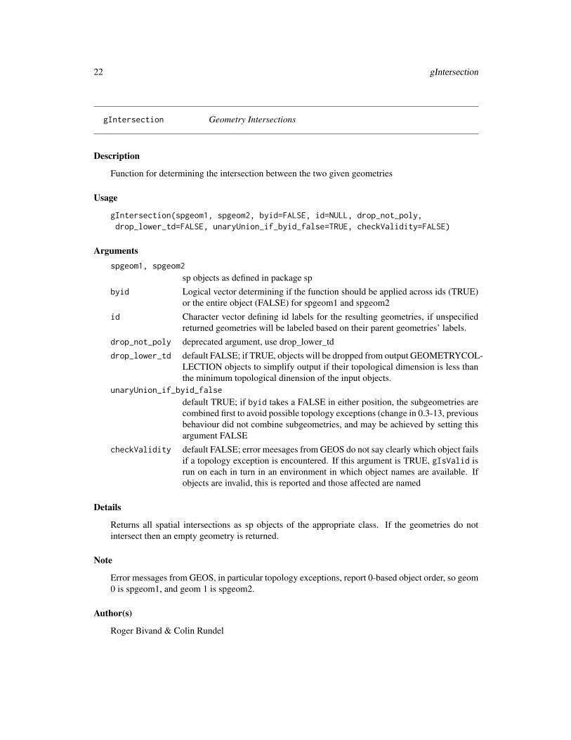
Function for determining the intersection between the two given geometries
Usage
gIntersection(spgeom1, spgeom2, byid=FALSE, id=NULL, drop_not_poly,drop_lower_td=FALSE, unaryUnion_if_byid_false=TRUE, checkValidity=FALSE)
Argumentsspgeom1, spgeom2
sp objects as defined in package spbyid Logical vector determining if the function should be applied across ids (TRUE)
or the entire object (FALSE) for spgeom1 and spgeom2id Character vector defining id labels for the resulting geometries, if unspecified
returned geometries will be labeled based on their parent geometries’ labels.drop_not_poly deprecated argument, use drop_lower_tddrop_lower_td default FALSE; if TRUE, objects will be dropped from output GEOMETRYCOL-
LECTION objects to simplify output if their topological dimension is less thanthe minimum topological dinension of the input objects.
unaryUnion_if_byid_false
default TRUE; if byid takes a FALSE in either position, the subgeometries arecombined first to avoid possible topology exceptions (change in 0.3-13, previousbehaviour did not combine subgeometries, and may be achieved by setting thisargument FALSE
checkValidity default FALSE; error meesages from GEOS do not say clearly which object failsif a topology exception is encountered. If this argument is TRUE, gIsValid isrun on each in turn in an environment in which object names are available. Ifobjects are invalid, this is reported and those affected are named
Details
Returns all spatial intersections as sp objects of the appropriate class. If the geometries do notintersect then an empty geometry is returned.
Note
Error messages from GEOS, in particular topology exceptions, report 0-based object order, so geom0 is spgeom1, and geom 1 is spgeom2.
Author(s)
Roger Bivand & Colin Rundel

gIntersection 23
See Also
gDifference gSymdifference gUnion
Examples
if (require(maptools)) {xx <- readShapeSpatial(system.file("shapes/fylk-val-ll.shp", package="maptools")[1],proj4string=CRS("+proj=longlat +datum=WGS84"))
bbxx <- bbox(xx)wdb_lines <- system.file("share/wdb_borders_c.b", package="maptools")xxx <- Rgshhs(wdb_lines, xlim=bbxx[1,], ylim=bbxx[2,])$SPres <-gIntersection(xx, xxx)plot(xx, axes=TRUE)plot(xxx, lty=2, add=TRUE)plot(res, add=TRUE, pch=16,col='red')}pol <- readWKT(paste("POLYGON((-180 -20, -140 55, 10 0, -140 -60, -180 -20),","(-150 -20, -100 -10, -110 20, -150 -20))"))
library(sp)GT <- GridTopology(c(-175, -85), c(10, 10), c(36, 18))gr <- as(as(SpatialGrid(GT), "SpatialPixels"), "SpatialPolygons")try(res <- gIntersection(pol, gr, byid=TRUE))res <- gIntersection(pol, gr, byid=TRUE, drop_lower_td=TRUE)# Robert Hijmans difficult intersection caseload(system.file("test_cases/polys.RData", package="rgeos"))try(res <- gIntersection(a, b, byid=TRUE))res <- gIntersection(a, b, byid=TRUE, drop_lower_td=TRUE)unlist(sapply(slot(res, "polygons"), function(p) sapply(slot(p, "Polygons"), slot, "area")))# example from Pius Korner 2015-10-25poly1 <- SpatialPolygons(list(Polygons(list(Polygon(coords=matrix(c(0, 0, 2, 2, 0, 1, 1, 0),ncol=2, byrow=FALSE))), ID=c("a")), Polygons(list(Polygon(coords=matrix(c(0, 0, 2, 2, 2, 3, 3, 2),ncol=2, byrow=FALSE))), ID=c("b"))))
poly2 <- SpatialPolygons(list(Polygons(list(Polygon(coords=matrix(c(0, 0, 2, 2,1, 1, 1, 3, 3, 0, 0, 2), ncol=2, byrow=FALSE))), ID=c("c"))))
plot(poly1, border="orange")plot(poly2, border="blue", add=TRUE, lty=2, density=8, angle=30, col="blue")gI <- gIntersection(poly1, poly2, byid=TRUE, drop_lower_td=TRUE)plot(gI, add=TRUE, border="red", lwd=3)oT <- get_RGEOS_polyThreshold()oW <- get_RGEOS_warnSlivers()oD <- get_RGEOS_dropSlivers()set_RGEOS_polyThreshold(1e-3)set_RGEOS_warnSlivers(TRUE)res1 <- gIntersection(a, b, byid=TRUE, drop_lower_td=TRUE)unlist(sapply(slot(res1, "polygons"), function(p) sapply(slot(p, "Polygons"), slot, "area")))set_RGEOS_dropSlivers(TRUE)res2 <- gIntersection(a, b, byid=TRUE, drop_lower_td=TRUE)unlist(sapply(slot(res2, "polygons"), function(p) sapply(slot(p, "Polygons"), slot, "area")))set_RGEOS_dropSlivers(FALSE)oo <- gUnaryUnion(res1, c(rep("1", 3), "2", "3", "4"))unlist(sapply(slot(oo, "polygons"), function(p) sapply(slot(p, "Polygons"), slot, "area")))ooo <- gIntersection(b, oo, byid=TRUE)

24 gIntersects
gArea(ooo, byid=TRUE)unlist(sapply(slot(ooo, "polygons"), function(p) sapply(slot(p, "Polygons"), slot, "area")))set_RGEOS_dropSlivers(TRUE)ooo <- gIntersection(b, oo, byid=TRUE)gArea(ooo, byid=TRUE)unlist(sapply(slot(ooo, "polygons"), function(p) sapply(slot(p, "Polygons"), slot, "area")))set_RGEOS_polyThreshold(oT)set_RGEOS_warnSlivers(oW)set_RGEOS_dropSlivers(oD)# see thread https://stat.ethz.ch/pipermail/r-sig-geo/2015-September/023468.htmlPol1=rbind(c(0,0),c(0,10),c(10,10),c(10,0),c(0,0))Pol2=rbind(c(0,0),c(10,0),c(10,-10),c(0,-10),c(0,0))library(sp)Pols1=Polygons(list(Polygon(Pol1)),"Pols1")Pols2=Polygons(list(Polygon(Pol2)),"Pols2")MyLay=SpatialPolygons(list(Pols1,Pols2))Pol1l=Pol1+0.5Pol2l=Pol2+0.5Pols1l=Polygons(list(Polygon(Pol1l)),"Pols1l")Pols2l=Polygons(list(Polygon(Pol2l)),"Pols2l")MyLayl=SpatialPolygons(list(Pols1l,Pols2l))inter=gIntersection(MyLay, MyLayl)plot(MyLay)plot(MyLayl,add=TRUE)plot(inter, add=TRUE, border="green")try(gIntersection(MyLay, MyLayl, unaryUnion_if_byid_false=FALSE))Pol1=rbind(c(0,0),c(0,1),c(1,1),c(1,0),c(0,0))Pol2=rbind(c(0,0),c(1,0),c(1,-1),c(0,-1),c(0,0))Pols1=Polygons(list(Polygon(Pol1)),"Pols1")Pols2=Polygons(list(Polygon(Pol2)),"Pols2")MyLay=SpatialPolygons(list(Pols1,Pols2))Pol1l=Pol1+0.1Pol2l=Pol2+0.1Pols1l=Polygons(list(Polygon(Pol1l)),"Pols1l")Pols2l=Polygons(list(Polygon(Pol2l)),"Pols2l")MyLayl=SpatialPolygons(list(Pols1l,Pols2l))inter=gIntersection(MyLay, MyLayl, unaryUnion_if_byid_false=FALSE)gEquals(inter, MyLay)inter1=gIntersection(MyLay, MyLayl, unaryUnion_if_byid_false=TRUE)gEquals(inter1, MyLay)gEquals(inter, inter1)plot(MyLay, ylim=c(-1, 1.1))plot(MyLayl, add=TRUE)plot(inter, angle=45, density=10, add=TRUE)plot(inter1, angle=135, density=10, add=TRUE)inter2=gIntersection(MyLay, MyLayl)gEquals(inter2, MyLay)gEquals(inter1, inter2)
gIntersects Geometry Relationships - Intersects and Disjoint

gIntersects 25
Description
Function for testing if the geometries have at least one point in common or no points in common
Usage
gIntersects(spgeom1, spgeom2 = NULL, byid = FALSE, prepared=TRUE,returnDense=TRUE, checkValidity=FALSE)
gDisjoint(spgeom1, spgeom2 = NULL, byid = FALSE, returnDense=TRUE,checkValidity=FALSE)
Arguments
spgeom1, spgeom2
sp objects as defined in package sp. If spgeom2 is NULL then spgeom1 iscompared to itself.
byid Logical vector determining if the function should be applied across ids (TRUE)or the entire object (FALSE) for spgeom1 and spgeom2
prepared Logical determining if prepared geometry (spatially indexed) version of theGEOS function should be used. In general prepared geometries should be fasterthan the alternative.
returnDense default TRUE, if false returns a list of the length of spgeom1 of integer vec-tors listing the 1:length(spgeom2) indices which would be TRUE in the denselogical matrix representation; useful when the sizes of the byid=TRUE returnedmatrix is very large and it is sparse; essential when the returned matrix wouldbe too large
checkValidity default FALSE; error meesages from GEOS do not say clearly which object failsif a topology exception is encountered. If this argument is TRUE, gIsValid isrun on each in turn in an environment in which object names are available. Ifobjects are invalid, this is reported and those affected are named
Value
gIntersects returns TRUE if spgeom1 and spgeom2 have at least one point in common.
gDisjoint returns TRUE if spgeom1 and spgeom2 have no points in common.
Both return a conforming logical matrix if byid = TRUE.
Note
Error messages from GEOS, in particular topology exceptions, report 0-based object order, so geom0 is spgeom1, and geom 1 is spgeom2.
Author(s)
Roger Bivand & Colin Rundel

26 gIsEmpty
See Also
gContains gContainsProperly gCovers gCoveredBy gCrosses gEquals gEqualsExact gOverlapsgRelate gTouches gWithin
Examples
p1 = readWKT("POLYGON((0 0,1 0,1 1,0 1,0 0))")p2 = readWKT("POLYGON((0.5 1,0 2,1 2,0.5 1))")p3 = readWKT("POLYGON((0.5 0.5,0 1.5,1 1.5,0.5 0.5))")
l1 = readWKT("LINESTRING(0 3,1 1,2 2,3 0)")l2 = readWKT("LINESTRING(1 3.5,3 3,2 1)")l3 = readWKT("LINESTRING(-0.1 0,-0.1 1.1,1 1.1)")
pt1 = readWKT("MULTIPOINT(1 1,3 0,2 1)")pt2 = readWKT("MULTIPOINT(0 3,3 0,2 1)")pt3 = readWKT("MULTIPOINT(-0.2 0,1 -0.2,1.2 1,0 1.2)")
par(mfrow=c(3,2))plot(p1,col='blue',border='blue',ylim=c(0,2.5));plot(p2,col='black',add=TRUE,pch=16)title(paste("Intersects:",gIntersects(p1,p2),"\nDisjoint:",gDisjoint(p1,p2)))
plot(p1,col='blue',border='blue',ylim=c(0,2.5));plot(p3,col='black',add=TRUE,pch=16)title(paste("Intersects:",gIntersects(p1,p3),"\nDisjoint:",gDisjoint(p1,p3)))
plot(l1,col='blue');plot(pt1,add=TRUE,pch=16)title(paste("Intersects:",gIntersects(l1,pt1),"\nDisjoint:",gDisjoint(l1,pt1)))
plot(l1,col='blue');plot(pt2,add=TRUE,pch=16)title(paste("Intersects:",gIntersects(l1,pt2),"\nDisjoint:",gDisjoint(l1,pt2)))
plot(p1,col='blue',border='blue',xlim=c(-0.5,2),ylim=c(0,2.5))plot(l3,lwd=2,col='black',add=TRUE)title(paste("Intersects:",gIntersects(p1,l3),"\nDisjoint:",gDisjoint(p1,l3)))
plot(p1,col='blue',border='blue',xlim=c(-0.5,2),ylim=c(-0.5,2))plot(pt3,pch=16,col='black',add=TRUE)title(paste("Intersects:",gIntersects(p1,pt3),"\nDisjoint:",gDisjoint(p1,pt3)))
gIsEmpty Is Geometry Empty?

gIsEmpty 27
Description
Tests if the given geometry is empty
Usage
gIsEmpty(spgeom, byid = FALSE)
Arguments
spgeom sp object as defined in package sp
byid Logical determining if the function should be applied across subgeometries(TRUE) or the entire object (FALSE)
Details
Because no sp Spatial object may be empty, the function exists but cannot work, as readWKT is notpermitted to create an empty object.
Value
Returns TRUE if the given geometry is empty, FALSE otherwise.
Author(s)
Roger Bivand & Colin Rundel
See Also
gIsRing gIsSimple gIsValid
Examples
try(gIsEmpty(readWKT("POINT EMPTY")))gIsEmpty(readWKT("POINT(1 1)"))try(gIsEmpty(readWKT("LINESTRING EMPTY")))gIsEmpty(readWKT("LINESTRING(0 0,1 1)"))try(gIsEmpty(readWKT("POLYGON EMPTY")))gIsEmpty(readWKT("POLYGON((0 0,1 0,1 1,0 1,0 0))"))

28 gIsRing
gIsRing Is Geometry a Ring?
Description
Tests if the given geometry is a ring
Usage
gIsRing(spgeom, byid = FALSE)
Arguments
spgeom sp object as defined in package spbyid Logical determining if the function should be applied across subgeometries
(TRUE) or the entire object (FALSE)
Value
Returns TRUE if the geometry is a LINEARRING.
Returns TRUE if the geometry is a LINESTRING that is both Simple (gIsSimple) and Closed (endpoints intersect), FALSE otherwise.
Returns FALSE if the geometry is a [MULTI]POINT, MULTILINESTRING, or [MULTI]POLYGON.
Author(s)
Roger Bivand & Colin Rundel
See Also
gIsEmpty gIsSimple gIsValid
Examples
l1 = readWKT("LINESTRING(0 0, 1 1, 1 0, 0 1, 0 0)")l2 = readWKT("LINESTRING(0 0,1 0,1 1,0 1,0 0)")r1 = readWKT("LINEARRING(0 0, 1 1, 1 0, 0 1, 0 0)")r2 = readWKT("LINEARRING(0 0,1 0,1 1,0 1,0 0)")p1 = readWKT("POLYGON((0 0, 1 1, 1 0, 0 1, 0 0))")p2 = readWKT("POLYGON((0 0,1 0,1 1,0 1,0 0))")
par(mfrow=c(3,2))plot(l1);title(paste("LINESTRING\nRing:",gIsRing(l1)))plot(l2);title(paste("LINESTRING\nRing:",gIsRing(l2)))plot(r1);title(paste("LINEARRING\nRing:",gIsRing(r1)))plot(r2);title(paste("LINEARRING\nRing:",gIsRing(r2)))plot(p1);title(paste("POLYGON\nRing:",gIsRing(p1)))plot(p2);title(paste("POLYGON\nRing:",gIsRing(p2)))

gIsSimple 29
gIsSimple Is Geometry Simple?
Description
Function tests if the given geometry is simple
Usage
gIsSimple(spgeom, byid = FALSE)
Arguments
spgeom sp object as defined in package sp
byid Logical determining if the function should be applied across subgeometries(TRUE) or the entire object (FALSE)
Details
Simplicity is used in reference to 0 and 1-dimensional geometries ([MULTI]POINT and [MULTI]LINESTRING)whereas Validity (gIsValid) is used in reference to 2-dimensional geometries ([MULTI]POLYGON).
A POINT is always simple.
A MULTIPOINT is simple if no two points are identical.
A LINESTRING is simple if it does not pass through the same point twice (self intersection) exceptat the end points, in which case it is a ring (gIsRing).
A MULTILINESTRING is simple if all of its subgeometries are simple and none of the subgeome-tries intersect except at end points.
A [MULTI]POLYGON is simple by definition.
Many of the functions in rgeos expect simple/valid geometries and may exhibit unpredictable behav-ior if given an invalid geometry. Checking of validity/simplicity can be computationally expensivefor complex geometries and so is not done by default, any new geometries should be checked.
Value
Returns TRUE if the given geometry does not contain anomalous points, such as self intersectionor self tangency.
Author(s)
Roger Bivand & Colin Rundel
References
Validity Details: http://postgis.net/docs/manual-2.0/using_postgis_dbmanagement.html#OGC_Validity
30 gIsValid
See Also
gIsEmpty gIsRing gIsValid
Examples
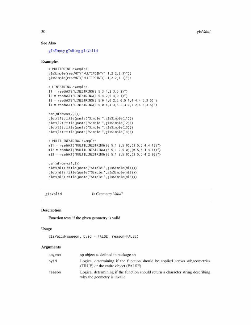
# MULTIPOINT examplesgIsSimple(readWKT("MULTIPOINT(1 1,2 2,3 3)"))gIsSimple(readWKT("MULTIPOINT(1 1,2 2,1 1)"))
# LINESTRING examplesl1 = readWKT("LINESTRING(0 5,3 4,2 3,5 2)")l2 = readWKT("LINESTRING(0 5,4 2,5 4,0 1)")l3 = readWKT("LINESTRING(3 5,0 4,0 2,2 0,5 1,4 4,4 5,3 5)")l4 = readWKT("LINESTRING(3 5,0 4,4 3,5 2,3 0,1 2,4 5,3 5)")
par(mfrow=c(2,2))plot(l1);title(paste("Simple:",gIsSimple(l1)))plot(l2);title(paste("Simple:",gIsSimple(l2)))plot(l3);title(paste("Simple:",gIsSimple(l3)))plot(l4);title(paste("Simple:",gIsSimple(l4)))
# MULTILINESTRING examplesml1 = readWKT("MULTILINESTRING((0 5,1 2,5 0),(3 5,5 4,4 1))")ml2 = readWKT("MULTILINESTRING((0 5,1 2,5 0),(0 5,5 4,4 1))")ml3 = readWKT("MULTILINESTRING((0 5,1 2,5 0),(3 5,5 4,2 0))")
par(mfrow=c(1,3))plot(ml1);title(paste("Simple:",gIsSimple(ml1)))plot(ml2);title(paste("Simple:",gIsSimple(ml2)))plot(ml3);title(paste("Simple:",gIsSimple(ml3)))
gIsValid Is Geometry Valid?
Description
Function tests if the given geometry is valid
Usage
gIsValid(spgeom, byid = FALSE, reason=FALSE)
Arguments
spgeom sp object as defined in package sp
byid Logical determining if the function should be applied across subgeometries(TRUE) or the entire object (FALSE)
reason Logical determining if the function should return a character string describingwhy the geometry is invalid

gIsValid 31
Details
Validity is used in reference to 2-dimensional geometries (LINEARRING and [MULTI]POLYGON)whereas Simplicity (gIsSimple) is used in reference to 0 and 1-dimensional geometries ([MULTI]POINTand [MULTI]LINESTRING).
A LINEARRING is valid if it does not intersect itself.
A POLYGON is valid if no two rings in the boundary (made up of an exterior ring and interiorrings) cross. The boundary of a POLYGON may intersect at a POINT but only as a tangent (i.e. noton a line). A POLYGON may not have cut lines or spikes and the interior rings must be containedentirely within the exterior ring.
A MULTIPOLYGON is valid if and only if all of its elements are valid and the interiors of no twoelements intersect. The boundaries of any two elements may touch, but only at a finite number ofPOINTs.
Many of the functions in rgeos expect simple/valid geometries and may exhibit unpredictable behav-ior if given an invalid geometry. Checking of validity/simplicity can be computationally expensivefor complex geometries and so is not done by default, any new geometries should be checked.
Value
By default will return TRUE if the given geometry is well formed, FALSE otherwise. If reason is setto TRUE then a character string is returned describing the geometry, "Valid Geometry" if it is validor details of the specific issue. Any given geometry may have multiple issues that make it invalid,gIsValid will only return the first, once it has been corrected additionally checking is necessary toconfirm that additional issues do not remain.
Author(s)
Roger Bivand & Colin Rundel
References
Validity Details: http://postgis.net/docs/manual-2.0/using_postgis_dbmanagement.html#OGC_Validity
See Also
gIsEmpty gIsRing gIsSimple
Examples
#LINEARRING Examplel = readWKT("LINEARRING(0 0, 100 100, 100 0, 0 100, 0 0)")plot(l);title(paste("Valid:",gIsValid(l),"\n",gIsValid(l,reason=TRUE)))
#POLYGON and MULTIPOLYGON Examplesp1 = readWKT("POLYGON ((0 60, 0 0, 60 0, 60 60, 0 60), (20 40, 20 20, 40 20, 40 40, 20 40))")p2 = readWKT("POLYGON ((0 60, 0 0, 60 0, 60 60, 0 60), (20 40, 20 20, 60 20, 20 40))")p3 = readWKT(paste("POLYGON ((0 120, 0 0, 140 0, 140 120, 0 120),","(100 100, 100 20, 120 20, 120 100, 100 100),",

32 gLength
"(20 100, 20 40, 100 40, 20 100))"))
p4 = readWKT("POLYGON ((0 40, 0 0, 40 40, 40 0, 0 40))")p5 = readWKT("POLYGON ((-10 50, 50 50, 50 -10, -10 -10, -10 50), (0 40, 0 0, 40 40, 40 0, 0 40))")p6 = readWKT("POLYGON ((0 60, 0 0, 60 0, 60 20, 100 20, 60 20, 60 60, 0 60))")p7 = readWKT(paste("POLYGON ((40 300, 40 20, 280 20, 280 300, 40 300),","(120 240, 80 180, 160 220, 120 240),","(220 240, 160 220, 220 160, 220 240),","(160 100, 80 180, 100 80, 160 100),","(160 100, 220 160, 240 100, 160 100))"))
p8 = readWKT(paste("POLYGON ((40 320, 340 320, 340 20, 40 20, 40 320),","(100 120, 40 20, 180 100, 100 120),","(200 200, 180 100, 240 160, 200 200),","(260 260, 240 160, 300 200, 260 260),","(300 300, 300 200, 340 320, 300 300))"))
p9 = readWKT(paste("MULTIPOLYGON (((20 380, 420 380, 420 20, 20 20, 20 380),","(220 340, 180 240, 60 200, 200 180, 340 60, 240 220, 220 340)),","((60 200, 340 60, 220 340, 60 200)))"))
par(mfrow=c(3,3))plot(p1,col='black',pbg='white');title(paste("Valid:",gIsValid(p1),"\n",gIsValid(p1,reason=TRUE)))plot(p2,col='black',pbg='white');title(paste("Valid:",gIsValid(p2),"\n",gIsValid(p2,reason=TRUE)))plot(p3,col='black',pbg='white');title(paste("Valid:",gIsValid(p3),"\n",gIsValid(p3,reason=TRUE)))plot(p4,col='black',pbg='white');title(paste("Valid:",gIsValid(p4),"\n",gIsValid(p4,reason=TRUE)))plot(p5,col='black',pbg='white');title(paste("Valid:",gIsValid(p5),"\n",gIsValid(p5,reason=TRUE)))plot(p6,col='black',pbg='white');title(paste("Valid:",gIsValid(p6),"\n",gIsValid(p6,reason=TRUE)))plot(p7,col='black',pbg='white');title(paste("Valid:",gIsValid(p7),"\n",gIsValid(p7,reason=TRUE)))plot(p8,col='black',pbg='white');title(paste("Valid:",gIsValid(p8),"\n",gIsValid(p8,reason=TRUE)))plot(p9,col='black',pbg='white')title(paste("Valid:",gIsValid(p9),"\n",gIsValid(p9,reason=TRUE)))
gLength Length of Geometry
Description
Calculates the length of the given geometry.
Usage
gLength(spgeom, byid=FALSE)
Arguments
spgeom sp object as defined in package sp
byid Logical determining if the function should be applied across subgeometries(TRUE) or the entire object (FALSE)

gNearestPoints 33
Value
Returns the length of the geometry in the units of the current projection. By definition [MULTI]POINTshave a length of 0. The length of POLYGONs is the sum of the length of their shell and their hole(s).
Author(s)
Roger Bivand & Colin Rundel
See Also
gArea
Examples
gLength(readWKT("POINT(1 1)"))
gLength(readWKT("LINESTRING(0 0,1 1,2 2)"))gLength(readWKT("LINESTRING(0 0,1 1,2 0,3 1)"))
gLength(readWKT("POLYGON((0 0,3 0,3 3,0 3,0 0))"))gLength(readWKT("POLYGON((0 0,3 0,3 3,0 3,0 0),(1 1,2 1,2 2,1 2,1 1))"))
gNearestPoints Closest Points of two Geometries
Description
Return closest points of two geometries.
Usage
gNearestPoints(spgeom1, spgeom2)
Arguments
spgeom1, spgeom2
sp objects as defined in package sp.
Value
The closest points of the two geometries or NULL on exception. The first point comes from sp-geom1 geometry and the second point comes from spgeom2.
Author(s)
Rainer Stuetz

34 gNode
See Also
gDistance
Examples
if (version_GEOS0() > "3.4.0") {g1 <- readWKT("MULTILINESTRING((34 54, 60 34), (0 10, 50 10, 100 50))")g2 <- readWKT("MULTIPOINT(30 0, 100 30)")plot(g1, pch=4, axes=TRUE)plot(g2, add=TRUE)plot(gNearestPoints(g1, g2), add=TRUE, col="red", pch=7)gDistance(g1, g2)}
gNode Linestring Noder
Description
Function attempts to node a linestring object, inserting coordinates at intersection points; only avail-able for GEOS >= 3.4.0.
Usage
gNode(spgeom);
Arguments
spgeom an sp object inheriting from SpatialLines
Details
Because gPolygonize expects linestrings to be fully noded, as such they must not cross and musttouch only at endpoints. gNodee takes an object inheriting from SpatialLines and attempts to addomitted nodes. Issue reported by Nicola Farina 21 March 2014.
Value
Returns a noded linestring object.
Author(s)
Roger Bivand
See Also
gPolygonize

gpc.poly-class 35
Examples
library(sp)pol1 <- readWKT(paste("POLYGON((39.936 43.446, 39.94 43.446, 39.94 43.45,","39.936 43.45, 39.936 43.446))"))
pol2 <- readWKT(paste("POLYGON((39.9417 43.45, 39.9395 43.4505,","39.9385 43.4462, 39.9343 43.4452, 39.9331 43.4469, 39.9417 43.45))"))
plot(pol2, axes=TRUE)plot(pol1, add=TRUE, border="blue")gIsValid(pol1)gIsValid(pol2)try(res <- gUnion(pol1, pol2))if (version_GEOS0() > "3.4.0") {pol2a <- gPolygonize(gNode(as(pol2, "SpatialLines")))try(res <- gUnion(pol1, pol2a))plot(res, add=TRUE, border="red", lty=2, lwd=2)set.seed(1)# rw from Jim Holtman's R-help posting 2010-12-2n <- 1000rw <- matrix(0, ncol = 2, nrow = n)indx <- cbind(seq(n), sample(c(1, 2), n, TRUE))rw[indx] <- sample(c(-1, 1), n, TRUE)rw[,1] <- cumsum(rw[, 1])rw[, 2] <- cumsum(rw[, 2])slrw <- SpatialLines(list(Lines(list(Line(rw)), "1")))res0 <- gNode(slrw)print(length(slrw))print(length(res0))res <- gPolygonize(res0)print(summary(res))print(length(res))plot(res0, axes=TRUE)plot(res, add=TRUE, col=sample(rainbow(length(res))))# library(spatstat)# set.seed(0)# X <- psp(runif(100), runif(100), runif(100), runif(100), window=owin())# library(maptools)# sppsp <- as(X, "SpatialLines")# writeLines(writeWKT(sppsp, byid=FALSE), con="sppsp.wkt")sppsp <- readWKT(readLines(system.file("wkts/sppsp.wkt", package="rgeos")))plot(sppsp, axes=TRUE)res0 <- gNode(sppsp)res <- gPolygonize(res0)plot(res, add=TRUE, col=sample(rainbow(length(res))))}
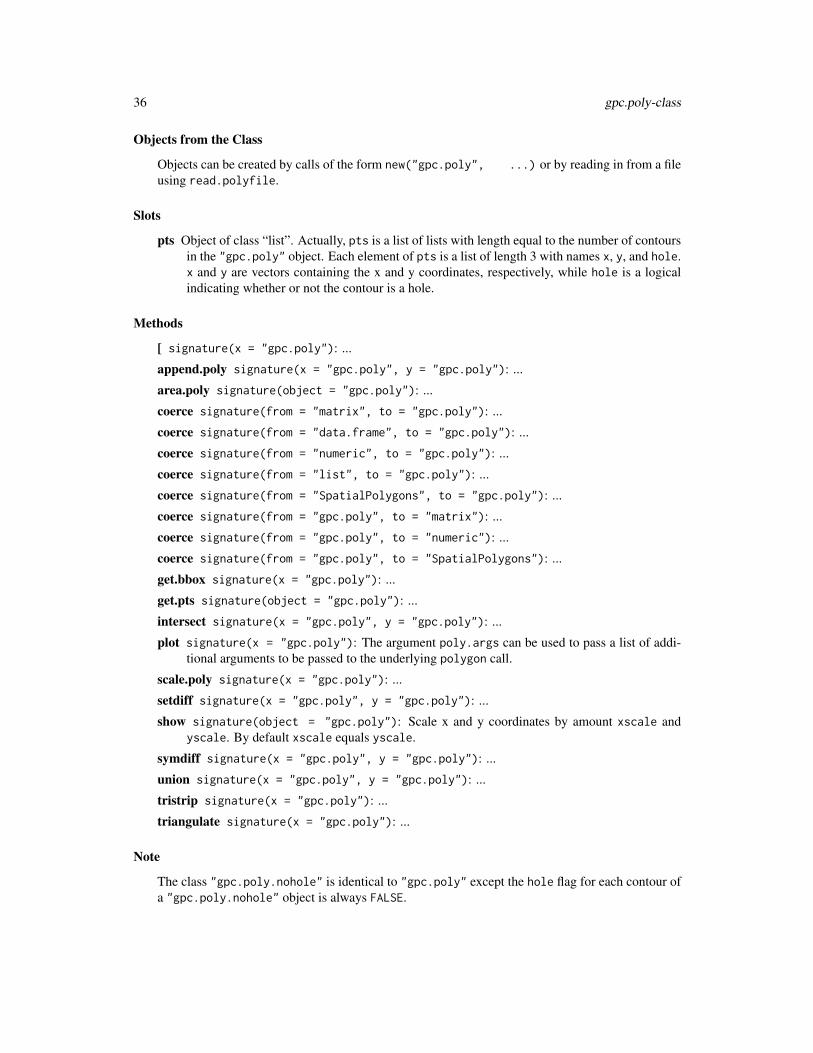
gpc.poly-class Class "gpc.poly"
Description
A class for representing polygons composed of multiple contours, some of which may be holes.
36 gpc.poly-class
Objects from the Class
Objects can be created by calls of the form new("gpc.poly", ...) or by reading in from a fileusing read.polyfile.
Slots
pts Object of class “list”. Actually, pts is a list of lists with length equal to the number of contoursin the "gpc.poly" object. Each element of pts is a list of length 3 with names x, y, and hole.x and y are vectors containing the x and y coordinates, respectively, while hole is a logicalindicating whether or not the contour is a hole.
Methods
[ signature(x = "gpc.poly"): ...
append.poly signature(x = "gpc.poly", y = "gpc.poly"): ...
area.poly signature(object = "gpc.poly"): ...
coerce signature(from = "matrix", to = "gpc.poly"): ...
coerce signature(from = "data.frame", to = "gpc.poly"): ...
coerce signature(from = "numeric", to = "gpc.poly"): ...
coerce signature(from = "list", to = "gpc.poly"): ...
coerce signature(from = "SpatialPolygons", to = "gpc.poly"): ...
coerce signature(from = "gpc.poly", to = "matrix"): ...
coerce signature(from = "gpc.poly", to = "numeric"): ...
coerce signature(from = "gpc.poly", to = "SpatialPolygons"): ...
get.bbox signature(x = "gpc.poly"): ...
get.pts signature(object = "gpc.poly"): ...
intersect signature(x = "gpc.poly", y = "gpc.poly"): ...
plot signature(x = "gpc.poly"): The argument poly.args can be used to pass a list of addi-tional arguments to be passed to the underlying polygon call.
scale.poly signature(x = "gpc.poly"): ...
setdiff signature(x = "gpc.poly", y = "gpc.poly"): ...
show signature(object = "gpc.poly"): Scale x and y coordinates by amount xscale andyscale. By default xscale equals yscale.
symdiff signature(x = "gpc.poly", y = "gpc.poly"): ...
union signature(x = "gpc.poly", y = "gpc.poly"): ...
tristrip signature(x = "gpc.poly"): ...
triangulate signature(x = "gpc.poly"): ...
Note
The class "gpc.poly.nohole" is identical to "gpc.poly" except the hole flag for each contour ofa "gpc.poly.nohole" object is always FALSE.

gpc.poly-class 37
Author(s)
Roger D. Peng
Examples
## Make some random polygonsset.seed(100)a <- cbind(rnorm(100), rnorm(100))a <- a[chull(a), ]
## Convert `a' from matrix to "gpc.poly"a <- as(a, "gpc.poly")
b <- cbind(rnorm(100), rnorm(100))b <- as(b[chull(b), ], "gpc.poly")
## More complex polygons with an intersectionp1 <- read.polyfile(system.file("poly-ex-gpc/ex-poly1.txt", package = "rgeos"))p2 <- read.polyfile(system.file("poly-ex-gpc/ex-poly2.txt", package = "rgeos"))
## Plot both polygons and highlight their intersection in redplot(append.poly(p1, p2))plot(intersect(p1, p2), poly.args = list(col = 2), add = TRUE)
## Highlight the difference p1 \ p2 in greenplot(setdiff(p1, p2), poly.args = list(col = 3), add = TRUE)
## Highlight the difference p2 \ p1 in blueplot(setdiff(p2, p1), poly.args = list(col = 4), add = TRUE)
## Plot the union of the two polygonsplot(union(p1, p2))
## Take the non-intersect portions and create a new polygon## combining the two contoursp.comb <- append.poly(setdiff(p1, p2), setdiff(p2, p1))plot(p.comb, poly.args = list(col = 2, border = 0))
## Coerce from a matrixx <-structure(c(0.0934073560027759, 0.192713393476752, 0.410062456627342,0.470020818875781, 0.41380985426787, 0.271408743927828, 0.100902151283831,0.0465648854961832, 0.63981588032221, 0.772382048331416,0.753739930955121, 0.637744533947066, 0.455466052934407,0.335327963176065, 0.399539700805524,0.600460299194476), .Dim = c(8, 2))y <-structure(c(0.404441360166551, 0.338861901457321, 0.301387925052047,0.404441360166551, 0.531852879944483, 0.60117973629424, 0.625537820957668,0.179976985040276, 0.341542002301496, 0.445109321058688,0.610817031070196, 0.596317606444189, 0.459608745684695,0.215189873417722), .Dim = c(7, 2))

38 gpc.poly.nohole-class
x1 <- as(x, "gpc.poly")y1 <- as(y, "gpc.poly")
plot(append.poly(x1, y1))plot(intersect(x1, y1), poly.args = list(col = 2), add = TRUE)
## Show the triangulation#plot(append.poly(x1, y1))#triangles <- triangulate(append.poly(x1,y1))#for (i in 0:(nrow(triangles)/3 - 1))# polygon(triangles[3*i + 1:3,], col="lightblue")
gpc.poly.nohole-class Class "gpc.poly.nohole"
Description
A class for representing polygons with multiple contours but without holes.
Objects from the Class
Objects can be created by calls of the form ‘new("gpc.poly.nohole", ...) or by calling read.polyfile’.
Slots
pts Object of class “list”. See the help for “gpc.poly” for details.
Extends
Class “gpc.poly”, directly.
Methods
coerce signature(from = "numeric", to = "gpc.poly.nohole"): ...
Note
This class is identical to “"gpc.poly"” and is needed because the file formats for polygons withoutholes is slightly different from the file format for polygons with holes. For a “gpc.poly.nohole”object, the hole flag for each contour is always FALSE.
Also, write.polyfile will write the correct file format, depending on whether the object is ofclass “gpc.poly” or “gpc.poly.nohole”.
Author(s)
Roger D. Peng

gPointOnSurface 39
See Also
gpc.poly-class
Examples
## None
gPointOnSurface Point on Surface of Geometry
Description
Function returns a point on the surface of the given geometry
Usage
gPointOnSurface(spgeom, byid=FALSE, id = NULL)
Arguments
spgeom sp object as defined in package sp
byid Logical determining if the function should be applied across subgeometries(TRUE) or the entire object (FALSE)
id Character vector defining id labels for the resulting geometries, if unspecifiedreturned geometries will be labeled based on their parent geometries’ labels.
Details
Returns a SpatialPoints object with a point that intersects with the geometry
Author(s)
Roger Bivand & Colin Rundel
See Also
gBoundary gCentroid gConvexHull gEnvelope
Examples
# Based on test geometries from JTSg1 = readWKT(paste("MULTIPOINT (60 300, 200 200, 240 240, 200 300, 40 140,","80 240, 140 240, 100 160, 140 200, 60 200)"))
g2 = readWKT("LINESTRING (0 0, 7 14)")g3 = readWKT("LINESTRING (0 0, 3 15, 6 2, 11 14, 16 5, 16 18, 2 22)")g4 = readWKT(paste("MULTILINESTRING ((60 240, 140 300, 180 200, 40 140, 100 100, 120 220),","(240 80, 260 160, 200 240, 180 340, 280 340, 240 180, 180 140, 40 200, 140 260))"))
g5 = readWKT("POLYGON ((0 0, 0 10, 10 10, 10 0, 0 0))")

40 gPolygonize
g6 = readWKT(paste("MULTIPOLYGON (((50 260, 240 340, 260 100, 20 60, 90 140, 50 260),","(200 280, 140 240, 180 160, 240 140, 200 280)),","((380 280, 300 260, 340 100, 440 80, 380 280),","(380 220, 340 200, 400 100, 380 220)))"))
par(mfrow=c(2,3))plot(g1); plot(gPointOnSurface(g1),col='red',add=TRUE)plot(g2); plot(gPointOnSurface(g2),col='red',add=TRUE)plot(g3); plot(gPointOnSurface(g3),col='red',add=TRUE)plot(g4); plot(gPointOnSurface(g4),col='red',add=TRUE)plot(g5); plot(gPointOnSurface(g5),col='red',add=TRUE)plot(g6); plot(gPointOnSurface(g6),col='red',add=TRUE)
gPolygonize Linestring Polygonizer
Description
Function attempts to polygonize the given list of linestrings. If the linestrings are not noded (co-ordinates inserted at intersection points), the function may fail. gNode may be tried to insert suchmissing points
Usage
gPolygonize( splist, getCutEdges=FALSE);
Arguments
splist a list of sp SpatialLines objects
getCutEdges Logical vector indicating if cut edges should be returned
Details
Polygonization is the process of forming polygons from linestrings which enclose an area. Linestringsare expected to be fully noded, as such they must not cross and must touch only at endpoints.gPolygonize takes a list of fully noded linestrings and forms all the polygons which are enclosedby the lines. Polygonization errors such as dangling lines or cut lines can be identified and reported.
Value
By default returns polygons generated by polygonizing the given linestrings. If getCutEdges isTRUE then any cut edges are returned.
Author(s)
Roger Bivand & Colin Rundel

gPolygonize 41
See Also
gNode
Examples
library(sp)linelist = list(readWKT("LINESTRING (0 0 , 10 10)"),readWKT("LINESTRING (185 221, 100 100)"),readWKT("LINESTRING (185 221, 88 275, 180 316)"),readWKT("LINESTRING (185 221, 292 281, 180 316)"),readWKT("LINESTRING (189 98, 83 187, 185 221)"),readWKT("LINESTRING (189 98, 325 168, 185 221)"))
par(mfrow=c(1,2))plot(linelist[[1]],xlim=c(0,350),ylim=c(0,350))title("Linestrings with nodes")plot(as(linelist[[1]],"SpatialPoints"),pch=16,add=TRUE)
for(i in 2:length(linelist)) {plot(linelist[[i]],add=TRUE)plot(as(linelist[[i]],"SpatialPoints"),pch=16,add=TRUE)}
plot(gPolygonize(linelist),xlim=c(0,350),ylim=c(0,350))title("Polygonized Results")
gPolygonize(linelist,getCutEdges=TRUE) # no cut edges
linelist2 = list(readWKT("LINESTRING(1 3, 3 3, 3 1, 1 1, 1 3)"),readWKT("LINESTRING(1 3, 3 3, 3 1, 1 1, 1 3)"))
gPolygonize(linelist2,getCutEdges=FALSE) # NULLgPolygonize(linelist2,getCutEdges=TRUE) # Contains LineStrings# bug fix 130206LS = list(readWKT("LINESTRING (425963 576719, 425980 576703)"),readWKT("LINESTRING (425963 576719, 425882 577073)"),readWKT("LINESTRING (425980 576703, 426082 577072)"),readWKT("LINESTRING (425882 577073, 426082 577072)"),readWKT("LINESTRING (426138 577068, 426082 577072)"),readWKT("LINESTRING (426138 577068, 426420 577039)"),readWKT("LINESTRING (426420 577039, 426554 576990)"),readWKT("LINESTRING (426751 576924, 426776 576823)"),readWKT("LINESTRING (426751 576924, 426783 576919)"),readWKT("LINESTRING (426751 576924, 426714 576953)"),readWKT("LINESTRING (426776 576823, 426783 576919)"),readWKT("LINESTRING (426658 576966, 426554 576990)"),readWKT("LINESTRING (426658 576966, 426667 577031)"),readWKT("LINESTRING (426658 576966, 426714 576953)"),readWKT("LINESTRING (426667 577031, 426714 576953)")

42 gProject
)plot(gPolygonize(LS))
gProject Project Points to Line Geometry
Description
Return distances along geometry to points nearest the specified points.
Usage
gProject(spgeom, sppoint, normalized = FALSE)
Arguments
spgeom SpatialLines or SpatialLinesDataFrame object
sppoint SpatialPoints or SpatialPointsDataFrame object
normalized Logical determining if normalized distances should be used
Details
If normalized=TRUE, distances normalized to the length of the geometry are returned, i.e., valuesbetween 0 and 1.
Value
a numeric vector containing the distances along the line to points nearest to the specified points
Author(s)
Rainer Stuetz
See Also
gInterpolate
Examples
l <- readWKT("LINESTRING(0 1, 3 4, 5 6)")p1 <- readWKT("MULTIPOINT(3 2, 3 5)")frac <- gProject(l, p1)p2 <- gInterpolate(l, frac)plot(l, axes=TRUE)plot(p1, col = "blue", add = TRUE)plot(p2, col = "red", add = TRUE)

gRelate 43
gRelate Geometry Relationships - Intersection Matrix Pattern (DE-9IM)
Description
Determines the relationships between two geometries by comparing the intersection of Interior,Boundary and Exterior of both geometries to each other. The results are summarized by the Dimen-sionally Extended 9-Intersection Matrix or DE-9IM.
Usage
gRelate(spgeom1, spgeom2 = NULL, pattern = NULL, byid = FALSE,checkValidity=FALSE)
Arguments
spgeom1, spgeom2
sp objects as defined in package sp. If spgeom2 is NULL then spgeom1 iscompared to itself.
byid Logical vector determining if the function should be applied across ids (TRUE)or the entire object (FALSE) for spgeom1 and spgeom2
pattern Character string containing intersection matrix pattern to match against DE-9IMfor given geometries. Wild card * or * characters allowed.
checkValidity default FALSE; error meesages from GEOS do not say clearly which object failsif a topology exception is encountered. If this argument is TRUE, gIsValid isrun on each in turn in an environment in which object names are available. Ifobjects are invalid, this is reported and those affected are named
Details
Each geometry is decomposed into an interior, a boundary, and an exterior region, all the result-ing geometries are then tested by intersection against one another resulting in 9 total comparisons.These comparisons are summarized by the dimensions of the intersection region, as such intersec-tion at point(s) is labeled 0, at linestring(s) is labeled 1, at polygons(s) is labeled 2, and if they donot intersect labeled F.
If a pattern is specified then limited matching with wildcards is possible, * matches any characterwhereas T matches any non-F character.
See references for additional details.
Value
By default returns a 9 character string that represents the DE-9IM.
If pattern returns TRUE if the pattern matches the DE-9IM.

44 gRelate
Note
Error messages from GEOS, in particular topology exceptions, report 0-based object order, so geom0 is spgeom1, and geom 1 is spgeom2.
Author(s)
Roger Bivand & Colin Rundel
References
Documentation of Intersection Matrix Patterns: http://docs.geotools.org/stable/userguide/library/jts/dim9.html
See Also
gContains gContainsProperly gCovers gCoveredBy gCrosses gDisjoint gEquals gEqualsExactgIntersects gOverlaps gTouches gWithin
Examples
x = readWKT("POLYGON((1 0,0 1,1 2,2 1,1 0))")x.inter = xx.bound = gBoundary(x)
y = readWKT("POLYGON((2 0,1 1,2 2,3 1,2 0))")y.inter = yy.bound = gBoundary(y)
xy.inter = gIntersection(x,y)xy.inter.bound = gBoundary(xy.inter)
xy.union = gUnion(x,y)bbox = gBuffer(gEnvelope(xy.union),width=0.5,joinStyle='mitre',mitreLimit=3)
x.exter = gDifference(bbox,x)y.exter = gDifference(bbox,y)
# geometry decompositionpar(mfrow=c(2,3))plot(bbox,border='grey');plot(x,col="black",add=TRUE);title("Interior",ylab = "Polygon X")plot(bbox,border='grey');plot(x.bound,col="black",add=TRUE);title("Boundary")plot(bbox,border='grey');plot(x.exter,col="black",pbg='white',add=TRUE);title("Exterior")plot(bbox,border='grey');plot(y,col="black",add=TRUE);title(ylab = "Polygon Y")plot(bbox,border='grey');plot(y.bound,col="black",add=TRUE)plot(bbox,border='grey');plot(y.exter,col="black",pbg='white',add=TRUE)
defaultplot = function() {plot(bbox,border='grey')
gSimplify 45
plot(x,add=TRUE,col='red1',border="red3")plot(y,add=TRUE,col='blue1',border="blue3")plot(xy.inter,add=TRUE,col='orange1',border="orange3")}
# Dimensionally Extended 9-Intersection Matrixpat = gRelate(x,y)patchars = strsplit(pat,"")[[1]]
par(mfrow=c(3,3))defaultplot(); plot(gIntersection(x.inter,y.inter),add=TRUE,col='black')title(paste("dim:",patchars[1]))defaultplot(); plot(gIntersection(x.bound,y.inter),add=TRUE,col='black',lwd=2)title(paste("dim:",patchars[2]))defaultplot(); plot(gIntersection(x.exter,y.inter),add=TRUE,col='black')title(paste("dim:",patchars[3]))
defaultplot(); plot(gIntersection(x.inter,y.bound),add=TRUE,col='black',lwd=2)title(paste("dim:",patchars[4]))defaultplot(); plot(gIntersection(x.bound,y.bound),add=TRUE,col='black',pch=16)title(paste("dim:",patchars[5]))defaultplot(); plot(gIntersection(x.exter,y.bound),add=TRUE,col='black',lwd=2)title(paste("dim:",patchars[6]))
defaultplot(); plot(gIntersection(x.inter,y.exter),add=TRUE,col='black')title(paste("dim:",patchars[7]))defaultplot(); plot(gIntersection(x.bound,y.exter),add=TRUE,col='black',lwd=2)title(paste("dim:",patchars[8]))defaultplot(); plot(gIntersection(x.exter,y.exter),add=TRUE,col='black')title(paste("dim:",patchars[9]))
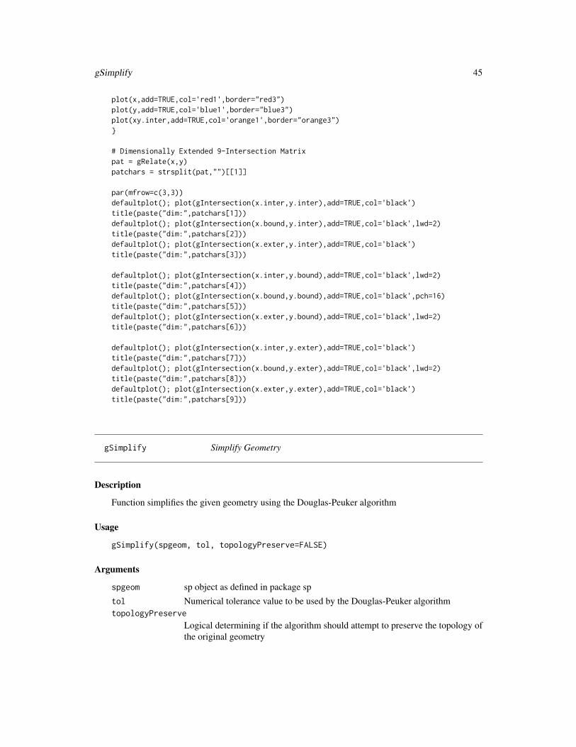
gSimplify Simplify Geometry
Description
Function simplifies the given geometry using the Douglas-Peuker algorithm
Usage
gSimplify(spgeom, tol, topologyPreserve=FALSE)
Arguments
spgeom sp object as defined in package sptol Numerical tolerance value to be used by the Douglas-Peuker algorithmtopologyPreserve
Logical determining if the algorithm should attempt to preserve the topology ofthe original geometry

46 gSymdifference
Details
When applied to lines it is possible for the resulting geometry to lose simplicity (gIsSimple). IftopologyPreserve is not specified it is also possible that the resulting geometries may no longerbe valid (gIsValid). Remember to check the resulting geometry as many other functions rely onsimplicity and or validity when performing their calculations.
Value
Returns a simplified version of the given geometry when applied to [MULTI]LINEs or [MULTI]POLYGONs.
Author(s)
Roger Bivand & Colin Rundel
References
Douglas-Peuker Algorithm: http://en.wikipedia.org/wiki/Ramer-Douglas-Peucker_algorithm
Examples
p = readWKT(paste("POLYGON((0 40,10 50,0 60,40 60,40 100,50 90,60 100,60","60,100 60,90 50,100 40,60 40,60 0,50 10,40 0,40 40,0 40))"))
l = readWKT("LINESTRING(0 7,1 6,2 1,3 4,4 1,5 7,6 6,7 4,8 6,9 4)")
par(mfrow=c(2,4))plot(p);title("Original")plot(gSimplify(p,tol=10));title("tol: 10")plot(gSimplify(p,tol=20));title("tol: 20")plot(gSimplify(p,tol=25));title("tol: 25")
plot(l);title("Original")plot(gSimplify(l,tol=3));title("tol: 3")plot(gSimplify(l,tol=5));title("tol: 5")plot(gSimplify(l,tol=7));title("tol: 7")par(mfrow=c(1,1))
gSymdifference Geometry Symmetric Difference
Description
Function for determining the symmetric difference between the two given geometries
Usage
gSymdifference(spgeom1, spgeom2, byid=FALSE, id=NULL, drop_lower_td=FALSE,unaryUnion_if_byid_false=TRUE, checkValidity=FALSE)

gSymdifference 47
Arguments
spgeom1, spgeom2
sp objects as defined in package sp
byid Logical vector determining if the function should be applied across ids (TRUE)or the entire object (FALSE) for spgeom1 and spgeom2
id Character vector defining id labels for the resulting geometries, if unspecifiedreturned geometries will be labeled based on their parent geometries’ labels.
drop_lower_td default FALSE; if TRUE, objects will be dropped from output GEOMETRYCOL-LECTION objects to simplify output if their topological dinension is less thanthe minimum topological dinension of the input objects.
unaryUnion_if_byid_false
default TRUE; if byid takes a FALSE in either position, the subgeometries arecombined first to avoid possible topology exceptions (change in 0.3-13, previousbehaviour did not combine subgeometries, and may be achieved by setting thisargument FALSE
checkValidity default FALSE; error meesages from GEOS do not say clearly which object failsif a topology exception is encountered. If this argument is TRUE, gIsValid isrun on each in turn in an environment in which object names are available. Ifobjects are invalid, this is reported and those affected are named
Details
Returns the regions of spgeom1 and spgeom2 that do not intersect. If the geometries do not intersectthen spgeom1 and spgeom2 will be returned as separate subgeometries.
Note
Error messages from GEOS, in particular topology exceptions, report 0-based object order, so geom0 is spgeom1, and geom 1 is spgeom2.
Author(s)
Roger Bivand & Colin Rundel
See Also
gDifference gIntersection gUnion
Examples
x = readWKT("POLYGON ((0 0, 0 10, 10 10, 10 0, 0 0))")y = readWKT("POLYGON ((5 5, 15 5, 15 15, 5 15, 5 5))")
d = gSymdifference(x,y)plot(d,col='red',pbg='white')
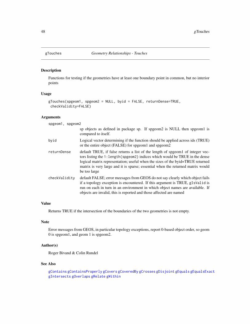
48 gTouches
gTouches Geometry Relationships - Touches
Description
Functions for testing if the geometries have at least one boundary point in common, but no interiorpoints
Usage
gTouches(spgeom1, spgeom2 = NULL, byid = FALSE, returnDense=TRUE,checkValidity=FALSE)
Argumentsspgeom1, spgeom2
sp objects as defined in package sp. If spgeom2 is NULL then spgeom1 iscompared to itself.
byid Logical vector determining if the function should be applied across ids (TRUE)or the entire object (FALSE) for spgeom1 and spgeom2
returnDense default TRUE, if false returns a list of the length of spgeom1 of integer vec-tors listing the 1:length(spgeom2) indices which would be TRUE in the denselogical matrix representation; useful when the sizes of the byid=TRUE returnedmatrix is very large and it is sparse; essential when the returned matrix wouldbe too large
checkValidity default FALSE; error meesages from GEOS do not say clearly which object failsif a topology exception is encountered. If this argument is TRUE, gIsValid isrun on each in turn in an environment in which object names are available. Ifobjects are invalid, this is reported and those affected are named
Value
Returns TRUE if the intersection of the boundaries of the two geometries is not empty.
Note
Error messages from GEOS, in particular topology exceptions, report 0-based object order, so geom0 is spgeom1, and geom 1 is spgeom2.
Author(s)
Roger Bivand & Colin Rundel
See Also
gContains gContainsProperly gCovers gCoveredBy gCrosses gDisjoint gEquals gEqualsExactgIntersects gOverlaps gRelate gWithin

gUnion 49
Examples
p1 = readWKT("POLYGON((0 0,1 0,1 1,0 1,0 0))")p2 = readWKT("POLYGON((0 1,0.5 2,1 1,0 1))")p3 = readWKT("POLYGON((0.5 1,0 2,1 2,0.5 1))")p4 = readWKT("POLYGON((0.5 0.5,0 1.5,1 1.5,0.5 0.5))")
l0 = readWKT("LINESTRING(0 1,0.5 2,1 1)")
l1 = readWKT("LINESTRING(0 0,2 2)")l2 = readWKT("LINESTRING(1 1,2 0)")l3 = readWKT("LINESTRING(0 2,2 0)")
par(mfrow=c(2,3))plot(p1,col='blue',border='blue',ylim=c(0,2.5));plot(p2,col='black',add=TRUE,pch=16)title(paste("Touches:",gTouches(p1,p2)))
plot(p1,col='blue',border='blue',ylim=c(0,2.5));plot(p3,col='black',add=TRUE,pch=16)title(paste("Touches:",gTouches(p1,p3)))
plot(p1,col='blue',border='blue',ylim=c(0,2.5));plot(p4,col='black',add=TRUE,pch=16)title(paste("Touches:",gTouches(p1,p4)))
plot(p1,col='blue',border='blue',ylim=c(0,2.5));plot(l0,lwd=2,col='black',add=TRUE,pch=16)title(paste("Touches:",gTouches(p1,l0)))
plot(l1,lwd=2,col='blue');plot(l2,lwd=2,col='black',add=TRUE,pch=16)title(paste("Touches:",gTouches(l1,l2)))
plot(l1,lwd=2,col='blue');plot(l3,lwd=2,col='black',add=TRUE,pch=16)title(paste("Touches:",gTouches(l1,l3)))
gUnion Geometry Union
Description
Functions for joining intersecting geometries.
Usage
gUnion(spgeom1, spgeom2, byid=FALSE, id=NULL, drop_lower_td=FALSE,unaryUnion_if_byid_false=TRUE, checkValidity=FALSE)
gUnionCascaded(spgeom, id = NULL)gUnaryUnion(spgeom, id = NULL)gLineMerge(spgeom, byid=FALSE, id = NULL)
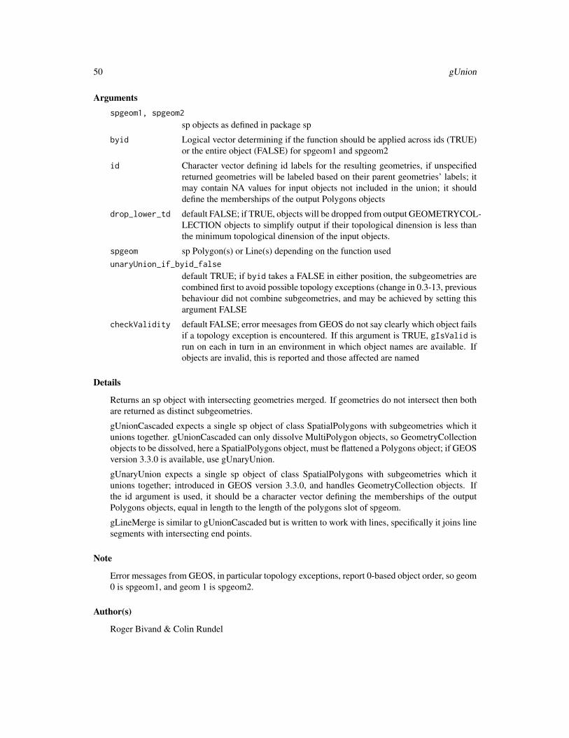
50 gUnion
Argumentsspgeom1, spgeom2
sp objects as defined in package sp
byid Logical vector determining if the function should be applied across ids (TRUE)or the entire object (FALSE) for spgeom1 and spgeom2
id Character vector defining id labels for the resulting geometries, if unspecifiedreturned geometries will be labeled based on their parent geometries’ labels; itmay contain NA values for input objects not included in the union; it shoulddefine the memberships of the output Polygons objects
drop_lower_td default FALSE; if TRUE, objects will be dropped from output GEOMETRYCOL-LECTION objects to simplify output if their topological dinension is less thanthe minimum topological dinension of the input objects.
spgeom sp Polygon(s) or Line(s) depending on the function usedunaryUnion_if_byid_false
default TRUE; if byid takes a FALSE in either position, the subgeometries arecombined first to avoid possible topology exceptions (change in 0.3-13, previousbehaviour did not combine subgeometries, and may be achieved by setting thisargument FALSE
checkValidity default FALSE; error meesages from GEOS do not say clearly which object failsif a topology exception is encountered. If this argument is TRUE, gIsValid isrun on each in turn in an environment in which object names are available. Ifobjects are invalid, this is reported and those affected are named
Details
Returns an sp object with intersecting geometries merged. If geometries do not intersect then bothare returned as distinct subgeometries.
gUnionCascaded expects a single sp object of class SpatialPolygons with subgeometries which itunions together. gUnionCascaded can only dissolve MultiPolygon objects, so GeometryCollectionobjects to be dissolved, here a SpatialPolygons object, must be flattened a Polygons object; if GEOSversion 3.3.0 is available, use gUnaryUnion.
gUnaryUnion expects a single sp object of class SpatialPolygons with subgeometries which itunions together; introduced in GEOS version 3.3.0, and handles GeometryCollection objects. Ifthe id argument is used, it should be a character vector defining the memberships of the outputPolygons objects, equal in length to the length of the polygons slot of spgeom.
gLineMerge is similar to gUnionCascaded but is written to work with lines, specifically it joins linesegments with intersecting end points.
Note
Error messages from GEOS, in particular topology exceptions, report 0-based object order, so geom0 is spgeom1, and geom 1 is spgeom2.
Author(s)
Roger Bivand & Colin Rundel

new-generics 51
See Also
gDifference gIntersection gSymdifference
Examples
if (require(maptools)) {nc1 <- readShapePoly(system.file("shapes/sids.shp", package="maptools")[1],proj4string=CRS("+proj=longlat +datum=NAD27"))
lps <- coordinates(nc1)ID <- cut(lps[,1], quantile(lps[,1]), include.lowest=TRUE)if (version_GEOS0() < "3.3.0") {
reg4 <- gUnionCascaded(nc1, ID)} else {
reg4 <- gUnaryUnion(nc1, ID)}row.names(reg4)par(mfrow=c(2,1))plot(nc1)plot(reg4)par(mfrow=c(1,1))}gt <- GridTopology(c(0.05,0.05), c(0.1,0.1), c(2,2))set.seed(1)xv <- rnorm(length(coordinates(gt)[,1]))xvs <- ifelse(xv > 0.2,1,0)grd <- SpatialGridDataFrame(gt, data.frame(xvs))spix <- as(grd, "SpatialPixelsDataFrame")spol <- as(spix, "SpatialPolygonsDataFrame")image(grd, axes=TRUE)if (version_GEOS0() < "3.3.0") {
spol1 <- gUnionCascaded(spol, as.character(spol$xvs))} else {
spol1 <- gUnaryUnion(spol, as.character(spol$xvs))}plot(spol1, add=TRUE)
new-generics Generics/Methods for polygon objects
Description
Some generic functions and methods for polygon objects
Usage
append.poly(x, y)area.poly(object, ...)get.pts(object)

52 new-generics
get.bbox(x)scale.poly(x, ...)tristrip(x)triangulate(x)
Arguments
x,object A polygon object
y A polygon object
... Other arguments passed to methods
Details
The result of tristrip(x) is a list of two-column matrices. Each matrix is a tristrip, i.e. the rowsare vertices of triangles, with each overlapping triple of rows corresponding to a separate triangle.
The result of triangulate(x) is a single two-column matrix. The rows are vertices of triangles,taken in non-overlapping triples.
Methods
append.poly signature(x = "gpc.poly", y = "gpc.poly"): Combine all contours of two"gpc.poly" objects and return the combined polygon as a "gpc.poly" object.
area.poly signature(object = "gpc.poly"): Compute and return the sum of the areas of allcontours in a "gpc.poly" object.
scale.poly signature(x = "gpc.poly"): Scale (divide) the x and y coordinates of a "gpc.poly"object by the amount xscale and yscale, respectively. Return a scaled "gpc.poly" object.
get.pts signature(object = "gpc.poly"): Return the list of x and y coordinates of the verticesof a "gpc.poly" object.
get.bbox signature(x = "gpc.poly"): Return the bounding box for a "gpc.poly" object.
tristrip signature(x = "gpc.poly"): Return a tristrip list for a "gpc.poly" object.
triangulate signature(x = "gpc.poly"): Return a matrix of vertices of a triangulation of a"gpc.poly" object.
Author(s)
Roger D. Peng; GPC Library by Alan Murta; tristrip additions by Duncan Murdoch
See Also
"gpc.poly" class documentation.
Examples
holepoly <- read.polyfile(system.file("poly-ex-gpc/hole-poly.txt",package ="rgeos"), nohole = FALSE)
area.poly(holepoly)stopifnot(area.poly(holepoly) == 8)

over 53
over Find spatial join or intersections
Description
Find spatial join or intersections
Usage
overGeomGeom(x, y, returnList = FALSE, fn = NULL, ..., minDimension = -1)overGeomGeomDF(x, y, returnList = FALSE, fn = NULL, ..., minDimension = -1)
Arguments
x see over
y see over
returnList see over
fn see over
... see over
minDimension integer; if -1, gIntersects is used to find geometry intersections; if 0, 1 or 2,gRelate is used. if gRelate is used, intersecting geometries are ordered by thedimension of the intersection (2: area overlap; 1: line in common; 0: point incommon), and minDimension determines the mininum dimension of intersec-tion required.
Value
see over
Note
gRelate (minDimension > -1) is likely to be substantially slower than gIntersects.
Author(s)
Edzer Pebesma
Examples
p1 = readWKT("POLYGON((0 1,0.95 0.31,0.59 -0.81,-0.59 -0.81,-0.95 0.31,0 1))")p2 = readWKT("POLYGON((2 2,-2 2,-2 -2,2 -2,2 2),(1 1,-1 1,-1 -1,1 -1,1 1))")
overGeomGeom(p1,p2)

54 polyfile
polyfile Read/Write polygon data
Description
Read/Write polygon and contour information from/to a text file.
Usage
read.polyfile(filename, nohole = TRUE)write.polyfile(poly, filename = "GPCpoly.txt")
Arguments
filename the name of the file (a character string) from/to which data should be read/written.
nohole Is this a polygon without holes?
poly an object of class "gpc.poly"
Details
The text file representation of a polygon is of the following format:
<number of contours><number of points in first contour>x1 y1x2 y2...<number of points in second contour>x1 y1x2 y2...
For example, a data file for a polygon with 2 contours (a four-sided object and a triangle) mightlook like:
241.0 1.01.0 2.03.4 3.2110 11.2321.0 11.222.3 99.24.5 5.4
The vertices of the polygon can be ordered either clockwise or counter-clockwise.

polyfile 55
If a polygon has contours which are holes, then the format is slightly different. Basically, a flag isset to indicate that a particular contour is a hole. The format is
<number of contours><number of points in first contour><hole flag>x1 y1x2 y2...<number of points in second contour><hole flag>x1 y1x2 y2...
The hole flag is either 1 to indicate a hole, or 0 for a regular contour. For example, a four-sidedpolygon with a triangular hole would be written as:
2314.0 4.06.0 5.05.0 6.0402.0 1.08.0 2.07.0 9.01.0 7.0
Value
If nohole is TRUE (the default) read.polyfile returns an object of class "gpc.poly.nohole".This object has the hole flag set to FALSE for all contours. If nohole is FALSE, then an object ofclass "gpc.poly" is returned.
write.polyfile does not return anything useful.
Author(s)
Roger D. Peng
See Also
gpc.poly-class, gpc.poly.nohole-class
Examples
## None right now.

56 polygonsLabel
polygonsLabel Compute optimal label positions for polygons
Description
Compute optimal positions for placing labels inside polygons, and optionally plot the labels. Vari-ous algorithms for finding the ‘optimal’ label positions are supported.
Usage
polygonsLabel(pols, labels = NULL, method = c("maxdist","buffer", "centroid", "random", "inpolygon")[1],gridpoints = 60, polypart = c("all", "largest")[1],cex = 1, doPlot = TRUE, ...)
Arguments
pols Object of class, or deriving from, SpatialPolygons.
labels Character vector of labels. Will be recycled to have the same number of elementsas the number of polygons in pols. If labels is NULL or empty, the label boxis taken as a square with sides equal to the current line height (see the cexargument).
method The method(s) to use when finding label positions. Will be recycled. Validmethods are maxdist (currently the default), buffer, centroid, random andinpolygon.
gridpoints Number of grid points to use for the initial grid search in the maxdist method.
polypart Should all (default) or only the largest polygon part of each polygon in polsbe used for the calculations? Will be recycled. Setting this to largest is veryuseful when labelling detailed coastlines of a country, consisting of a large poly-gon (where the label should be placed) and very many tiny islands, as it willgreatly speed up the search for an optimal label position. But do note that thisalso removes any holes (e.g., lakes) before calculating the label position, so thelabels are no longer guaranteed not to overlap a hole.
cex Magnification factor for text labels. Is used both when plotting the labels andwhen calculating the label positions.
doPlot Plot the labels on the current graphics device. Calls the text function internally.
... Further arguments to be passed to text (e.g., col).
Details
There are no perfect definitions of ‘optimal’ label positions, but any such position should at leastsatisfy a few requirements: The label should be positioned wholly inside the polygon. It shouldalso be far from any polygon edges. And, though more difficult to quantify, it should be positionedin the visual centre (or bulk) of the polygon. The algorithms implemented here seems to generallydo a very good job of finding optimal (or at least ‘good’) label positions.

polygonsLabel 57
The maxdist method is currently the default, and tries to find the label position with a maximaldistance from the polygon edges. More precisely, it finds a position where the minimal distance ofany point on the (rectangular) label box to the polygon boundary is maximised. It does this by firsttrying a grid search, using gridpoints regular grid points on the polygon, and then doing localoptimisation on the best grid point. The default grid is quite coarse, but usually gives good resultsin a short amount of time. But for very complicated (and narrow) polygons, it may help increasinggridpoints. Note that while this method gives good results for most natural polygons, e.g., countryoutlines, the theoretical optimal position is not necessarily unique, and this is sometimes seen whenapplying the method to regular polygons, like rectangles (see example below), where the resultingposition may differ much from what one would judge to be the visual centre of the polygon.
The buffer method works by shrinking the polygon (using negative buffering) until the convex hullof the shrunken polygon can fit wholly inside the original polygon. The label position is then takenas the centroid of the shrunken polygon. This method usually gives excellent results, is surprisinglyfast, and seems to capture the ‘visual centre’ idea of an optimal label position well. However, itdoes not guarantee that the label can fit wholly inside the polygon. (However, if it does not fit, thereare usually no other better position either.)
The centroid method simply returns the centroid of each polygon. Note that although this is thegeometrical/mathematical centre of the polygon, it may actually be positioned outside the polygon.For regular polygons (rectangles, hexagons), it gives perfect results. Internally, this method usesthe coordinates function. There are three reasons this method is supported: To make it easy tofind the centroid of the largest polygon part of a polygon (using the polypart argument), to makeit easy to use the centroid algorithm along with other algorithms (using the vector nature of themethod argument), and for completeness.
The random method returns a random position guaranteed to be inside the polygon. This will rarelybe an optimal label position!
The inpolygon method finds an arbitrary position in the polygon. This position is usually quitesimilar to the centroid, but is guaranteed the be inside the polygon. Internally, the method uses thegPointOnSurface function.
Value
A two-colum matrix is returned, with each row containing the horizontal and vertical coordinatesfor the corresponding polygon. If doPlot is TRUE (the default), the labels are also plotted on thecurrent graphics device, with the given value of cex (font size scaling).
Note
Note that both the labels, method and polypart arguments are vectors, so it’s possible to usedifferent options for each polygon in the pols object.
Author(s)
Karl Ove Hufthammer, <[email protected]>.
References
The buffer method was inspired by (but is slightly different from) the algorithm described inthe paper Using Shape Analyses for Placement of Polygon Labels by Hoseok Kang and Shoreh

58 polygonsLabel
Elhami, available at http://training.esri.com/bibliography/index.cfm?event=general.recordDetail&ID=13608 .
See Also
pointLabel
Examples
# Simple example with a single polygonx = c(0, 1.8, 1.8, 1, 1, 3, 3, 2.2, 2.2, 4,
4, 6, 6, 14, 14, 6, 6, 4, 4, 0, 0)y = c(0, 0, -2, -2, -10, -10, -2, -2, 0, 0,
1.8, 1.8, 1, 1, 3, 3, 2.2, 2.2, 4, 4, 0)xy = data.frame(x,y)library(sp)xy.sp = SpatialPolygons(list(Polygons(list(Polygon(xy)), ID = "test")))plot(xy.sp, col = "khaki")polygonsLabel(xy.sp, "Hi!")
# Example with multiple polygons, text labels and coloursx1 = c(0, 4, 4, 0, 0)y1 = c(0, 0, 4, 4, 0)x2 = c(1, 1, 3, 3, 1)y2 = c(-2, -10, -10, -2, -2)x3 = c(6, 14, 14, 6, 6)y3 = c(1, 1, 3, 3, 1)xy.sp = SpatialPolygons(list(
Polygons(list(Polygon(cbind(x1,y1))), ID = "test1"), # boxPolygons(list(Polygon(cbind(x3,y3))), ID = "test3"), # widePolygons(list(Polygon(cbind(x2,y2))), ID = "test2") # high
))plot(xy.sp, col=terrain.colors(3))labels=c("Hi!", "A very long text string", "N\na\nr\nr\no\nw")
# Note that the label for the tall and narrow box is# not necessarily centred vertically in the box.# The reason is that method="maxdist" minimises the# maximum distance from the label box to the surrounding# polygon, and this distance is not changed by moving# the label vertically, as long the vertical distance# to the polygon boundary is less than the horizontal# distance. For regular polygons like this, the other# label positions (e.g., method="buffer") work better.polygonsLabel(xy.sp, labels, cex=.8,
col = c('white', 'black', 'maroon'))
## Not run:## Example showing how bad the centroid## position can be on real maps.

RGEOS Experimental Functions 59
# Needed librariesif (require(maps) && require(maptools) && require(rgdal)) {
# Load map data and convert to spatial objectnmap = map("world", c("Norway", "Sweden", "Finland"),
exact = TRUE, fill = TRUE, col = "transparent", plot = FALSE)nmap.pol = map2SpatialPolygons(nmap, IDs = nmap$names,
proj4string = CRS("+init=epsg:4326"))nmap.pol = spTransform(nmap.pol, CRS("+init=epsg:3035"))
# Plot map, centroid positions (red dots) and optimal# label positions using the ‘buffer’ method.plot(nmap.pol, col = "khaki")nmap.centroids = polygonsLabel(nmap.pol, names(nmap.pol),
method = "centroid", doPlot = FALSE)points(nmap.centroids, col = "red", pch=19)polygonsLabel(nmap.pol, names(nmap.pol), method = "buffer", cex=.8)}
## End(Not run)
RGEOS Experimental Functions
Experimental Functions
Description
Functions still under development using the GEOS STRtree structure to find intersecting objectcomponent envelopes (bounding boxes).
Usage
gUnarySTRtreeQuery(obj)gBinarySTRtreeQuery(obj1, obj2)poly_findInBoxGEOS(spl, as_points=TRUE)
Arguments
obj, obj1, obj2
Objects inheriting from either SpatialPolygons or SpatialLines, obj2 mayalso inherit from SpatialPoints
spl Object that inherits from the SpatialPolygons class
as_points Logical value indicating if the polygon should be treated as points

60 RGEOS Polygon Hole Comment Functions
Details
gUnarySTRtreeQuery and poly_findInBoxGEOS do the same thing, but poly_findInBoxGEOSuses the as_points argument to build the input envelopes from proper geometries. gUnarySTRtreeQueryand gBinarySTRtreeQuery build input envelopes by disregarding topology and reducing the coor-dinates to a multipoint representation. This permits the tree to be built and queried even when somegeometries are invalid. gUnarySTRtreeQuery and poly_findInBoxGEOS return a list of length(n-1) of 1-based indices only for the “greater than i” indices. gBinarySTRtreeQuery returns a listof the length of obj2 with 1-based indices of obj1.
Author(s)
Roger Bivand & Colin Rundel
Examples
if (require(maptools)) {xx <- readShapeSpatial(system.file("shapes/fylk-val-ll.shp",package="maptools")[1], proj4string=CRS("+proj=longlat +datum=WGS84"))
a0 <- gUnarySTRtreeQuery(xx)a0bbxx <- bbox(xx)wdb_lines <- system.file("share/wdb_borders_c.b", package="maptools")xxx <- Rgshhs(wdb_lines, xlim=bbxx[1,], ylim=bbxx[2,])$SPa1 <- gBinarySTRtreeQuery(xx, xxx)a1nc1 <- readShapePoly(system.file("shapes/sids.shp", package="maptools")[1],proj4string=CRS("+proj=longlat +datum=NAD27"))
a2 <- gUnarySTRtreeQuery(nc1)a3 <- poly_findInBoxGEOS(nc1)all.equal(a2, a3)a2pl <- slot(nc1, "polygons")[[4]]a5 <- gUnarySTRtreeQuery(pl)a5SG <- Sobj_SpatialGrid(nc1, n=400)$SGobj1 <- as(as(SG, "SpatialPixels"), "SpatialPolygons")a4 <- gBinarySTRtreeQuery(nc1, obj1)plot(nc1, col="orange", border="yellow")plot(obj1, angle=sapply(a4, is.null)*45, density=20, lwd=0.5, add=TRUE)set.seed(1)pts <- spsample(nc1, n=10, type="random")res <- gBinarySTRtreeQuery(nc1, pts)}
RGEOS Polygon Hole Comment Functions
RGEOS Polygon Hole Comment Functions

RGEOS Polygon Hole Comment Functions 61
Description
Utility functions for assigning ownership of holes to parent polygons
Usage
createSPComment(sppoly,which=NULL,overwrite=TRUE)createPolygonsComment(poly)
set_do_poly_check(value)get_do_poly_check()
Arguments
sppoly Object that inherits from the SpatialPolygons class
which Vector, which subset of geometries in sppoly should comment attributes be gen-erated
overwrite Logical, if a comment attribute already exists should it be overwritten
poly Object of class Polygons
value logical value to set “do_poly_check” option, default TRUE
Details
In order for rgeos to function properly it is necessary that all holes within a given POLYGONor MULTIPOLYGON geometry must belong to a specific polygon. The SpatialPolygons classimplementation does not currently include this information. To work around this limitation rgeosuses an additional comment attribute on the Polygons class that indicates which hole belongs towhich polygon.
Under the current implementation this comment is a text string of numbers separated by spaceswhere the order of the numbers corresponds to the order of the Polygon objects in the Polygonsslot of the Polygons object. A 0 implies the Polygon object is a polygon, a non-zero numberimplies that the Polygon object is a hole with the value indicating the index of the Polygon that“owns” the hole.
createPolygonsComment attempts to create a valid comment for a Polygons object by assessingwhich polygons contain a given hole (using gContains). Ownership is assigned to the smallestpolygon (by area) that contains the given hole. This is not guaranteed to generate valid polygons,always check the resulting objects for validity.
createSPComment attempts to create valid comments for all or a subset of polygons within aSpatialPolygons object.
Warning: check polygons
The helper functions get and set the imposition of checking of objects inheriting from SpatialPolygonsfor proper assignment of hole interior rings to exterior rings in Polygons objects. The internalGEOS representation defines a POLYGON object as a collection of only one exterior ring and fromzero to many interior rings, so an sp Polygons object corresponds to a GEOS MULTIPOLYGONobject, but without proper hole assignment. By default do_poly_check is TRUE; if it is set toFALSE using set_do_poly_check(FALSE), and the Polygons object is not valid in GEOS terms,GEOS may crash R, which is why checks are imposed by default.

62 RGEOS Polygon Hole Comment Functions
The details below show how hole assignment is handled in the package; here we assume that thehole status slots of all Polygon objects in a given Polygons object are set correctly. In the examplesbelow, we use a data set from maptools which has the holes correctly assigned, and we see thatthe SpatialPolygons object is geometrically valid both initially and after removing the commentattribute on the only Polygons object in usa - regenerating internally within rgeos from the holestatus slots since do_poly_check is TRUE.
If we modify usa by setting all hole status slots to FALSE, the SpatialPolygons object is geomet-rically invalid even though a comment attribute can be created - the function createSPComment isdeceived by the incorrect hole status slots. To rectify this, we use checkPolygonsHoles from map-tools on each Polygons object. This function calls gContains, gContainsProperly, gEquals andcreatePolygonsComment from rgeos to check whether the hole status slots are set correctly. Ex-perience shows that many imported datasets from for example publically provided shapefiles haveincorrect hole status values. Running checkPolygonsHoles is time-consuming when the numberof member Polygon objects is large - attempts will be made to make this more efficient.
Warning: planar geometries
The geometries handled by GEOS are assumed to be planar, so that any rgeos functions mak-ing measurements will give incorrect results when used on geographical coordinates measured indecimal degrees. Topological functions may work satisfactorily, but will not understand sphericalwrap-around.
Author(s)
Roger Bivand & Colin Rundel
Examples
library(sp)p1 <- Polygon(cbind(x=c(0, 0, 10, 10, 0), y=c(0, 10, 10, 0, 0)), hole=FALSE) # Ip2 <- Polygon(cbind(x=c(3, 3, 7, 7, 3), y=c(3, 7, 7, 3, 3)), hole=TRUE) # Hp8 <- Polygon(cbind(x=c(1, 1, 2, 2, 1), y=c(1, 2, 2, 1, 1)), hole=TRUE) # Hp9 <- Polygon(cbind(x=c(1, 1, 2, 2, 1), y=c(5, 6, 6, 5, 5)), hole=TRUE) # Hp3 <- Polygon(cbind(x=c(20, 20, 30, 30, 20), y=c(20, 30, 30, 20, 20)),hole=FALSE) # Ip4 <- Polygon(cbind(x=c(21, 21, 29, 29, 21), y=c(21, 29, 29, 21, 21)),hole=TRUE) # Hp5 <- Polygon(cbind(x=c(22, 22, 28, 28, 22), y=c(22, 28, 28, 22, 22)),hole=FALSE) # Ip6 <- Polygon(cbind(x=c(23, 23, 27, 27, 23), y=c(23, 27, 27, 23, 23)),hole=TRUE) # Hp7 <- Polygon(cbind(x=c(13, 13, 17, 17, 13), y=c(13, 17, 17, 13, 13)),hole=FALSE) # Ip10 <- Polygon(cbind(x=c(24, 24, 26, 26, 24), y=c(24, 26, 26, 24, 24)),hole=FALSE) # Ip11 <- Polygon(cbind(x=c(24.25, 24.25, 25.75, 25.75, 24.25),y=c(24.25, 25.75, 25.75, 24.25, 24.25)), hole=TRUE) # Hp12 <- Polygon(cbind(x=c(24.5, 24.5, 25.5, 25.5, 24.5),y=c(24.5, 25.5, 25.5, 24.5, 24.5)), hole=FALSE) # Ip13 <- Polygon(cbind(x=c(24.75, 24.75, 25.25, 25.25, 24.75),

RGEOS Utility Functions 63
y=c(24.75, 25.25, 25.25, 24.75, 24.75)), hole=TRUE) # H
lp <- list(p1, p2, p13, p7, p6, p5, p4, p3, p8, p11, p12, p9, p10)# 1 2 3 4 5 6 7 8 9 10 11 12 13# 0 1 11 0 6 0 8 0 1 13 0 1 0# I H H I H I H I H H I H Ipls <- Polygons(lp, ID="1")comment(pls)
comment(pls) = createPolygonsComment(pls)comment(pls)
plot(SpatialPolygons(list(pls)), col="magenta", pbg="cyan")title(xlab="Hole slot values before checking")
## Not run:# running this illustration may be time-consumingif (require(maptools)) {data(wrld_simpl)usa <- wrld_simpl[wrld_simpl$ISO3=="USA",]lapply(slot(usa, "polygons"), comment)gIsValid(usa, reason=TRUE)comment(slot(usa, "polygons")[[1]]) <- NULLlapply(slot(usa, "polygons"), comment)gIsValid(usa)any(c(sapply(slot(usa, "polygons"),function(x) sapply(slot(x, "Polygons"), slot, "hole"))))
lapply(slot(createSPComment(usa), "polygons"), comment)usa1 <- usaPls <- slot(usa1, "polygons")pls <- slot(Pls[[1]], "Polygons")pls1 <- lapply(pls, function(p) {slot(p, "hole") <- FALSE; return(p)})slot(Pls[[1]], "Polygons") <- pls1slot(usa1, "polygons") <- Plsany(c(sapply(slot(usa1, "polygons"),function(x) sapply(slot(x, "Polygons"), slot, "hole"))))
lapply(slot(createSPComment(usa1), "polygons"), comment)gIsValid(usa1, reason=TRUE)Pls <- slot(usa1, "polygons")Pls1 <- lapply(Pls, checkPolygonsHoles)slot(usa1, "polygons") <- Pls1lapply(slot(usa1, "polygons"), comment)gIsValid(usa1, reason=TRUE)}
## End(Not run)
RGEOS Utility Functions
RGEOS Utility Functions

64 RGEOS Utility Functions
Description
Utility functions for the RGEOS package
Usage
getScale()setScale(scale=100000000)translate(spgeom)checkP4S(p4s)
version_GEOS()rgeos_extSoftVersion()version_GEOS0()set_RGEOS_polyThreshold(value)get_RGEOS_polyThreshold()set_RGEOS_warnSlivers(value)get_RGEOS_warnSlivers()set_RGEOS_dropSlivers(value)get_RGEOS_dropSlivers()
Arguments
scale Numeric value determining the precision of translated geometries
spgeom sp object as defined in package sp
p4s Either a character string or an object of class CRS
value the value to be passed to an RGEOS option in its environment
Details
getScale and setScale are used to get and set the scale option in the rgeos environment. This optionis used to determine the precision of coordinates when translating to and from GEOS C objects.Precision is defined as 1 / scale. The final example is a use case reported by Mao-Gui Hu, whohas also made the objects available, where the default scale defeats an intended line intersectionoperation; changing the scale temporarily resoves the issue.
In order to permit polygon slivers to be detected, reported and dropped, the user may set a numericvalue for polyThreshold and logical values for warnSlivers and dropSlivers. By default, the thresh-old is 0.0, and warning and dropping are FALSE. To detect slivers, the threshold may be set toa small value and warnSlivers set to TRUE. To drop slivers from returned Polygons and Polygonobjects, set dropSlivers to TRUE for a non-zero threshold.
translate is a testing function which translates the sp object into a GEOS C object and then backinto an sp object and is used extensively in the translation unit tests. In all cases it is expected thatspgeom and translate(spgeom) should be identical.
checkP4S is a validation function for proj4strings and is used in testing.
version_GEOS returns the full runtime version string, and version_GEOS0 only the GEOS versionnumber.

RGEOS Utility Functions 65
Author(s)
Roger Bivand & Colin Rundel
Examples
readWKT("POINT(1.5 1.5)")
# With scale set to 1, the following point will be roundedsetScale(1)readWKT("POINT(1.5 1.5)")
setScale(10)readWKT("POINT(1.5 1.5)")
getScale()# Set scale option back to defaultsetScale()
# scale option only affect objects when they are translated through rgeossetScale(1)library(sp)SpatialPoints(data.frame(x=1.5,y=1.5))translate( SpatialPoints(data.frame(x=1.5,y=1.5)) )
setScale()
# added example of scale impact on intersection 120905sline1 <- readWKT(readLines(system.file("wkts/sline1.wkt", package="rgeos")))sline2 <- readWKT(readLines(system.file("wkts/sline2.wkt", package="rgeos")))rslt <- gIntersection(sline1, sline2)class(rslt)getScale()setScale(1e+6)rslt <- gIntersection(sline1, sline2)class(rslt)sapply(slot(rslt, "lines"), function(x) length(slot(x, "Lines")))rslt <- gLineMerge(rslt, byid=TRUE)sapply(slot(rslt, "lines"), function(x) length(slot(x, "Lines")))setScale()get_RGEOS_dropSlivers()get_RGEOS_warnSlivers()get_RGEOS_polyThreshold()# Robert Hijmans difficult intersection caseload(system.file("test_cases/polys.RData", package="rgeos"))try(res <- gIntersection(a, b, byid=TRUE))res <- gIntersection(a, b, byid=TRUE, drop_lower_td=TRUE)sort(unlist(sapply(slot(res, "polygons"), function(p) sapply(slot(p, "Polygons"), slot, "area"))))oT <- get_RGEOS_polyThreshold()oW <- get_RGEOS_warnSlivers()oD <- get_RGEOS_dropSlivers()

66 RGEOS WKT Functions
set_RGEOS_polyThreshold(1e-3)set_RGEOS_warnSlivers(TRUE)res1 <- gIntersection(a, b, byid=TRUE, drop_lower_td=TRUE)sort(unlist(sapply(slot(res, "polygons"), function(p) sapply(slot(p, "Polygons"), slot, "area"))))set_RGEOS_dropSlivers(TRUE)res2 <- gIntersection(a, b, byid=TRUE, drop_lower_td=TRUE)sort(unlist(sapply(slot(res, "polygons"), function(p) sapply(slot(p, "Polygons"), slot, "area"))))set_RGEOS_dropSlivers(FALSE)oo <- gUnaryUnion(res1, c(rep("1", 3), "2", "3", "4"))unlist(sapply(slot(oo, "polygons"), function(p) sapply(slot(p, "Polygons"), slot, "area")))ooo <- gIntersection(b, oo, byid=TRUE)gArea(ooo, byid=TRUE)unlist(sapply(slot(ooo, "polygons"), function(p) sapply(slot(p, "Polygons"), slot, "area")))set_RGEOS_dropSlivers(TRUE)ooo <- gIntersection(b, oo, byid=TRUE)gArea(ooo, byid=TRUE)unlist(sapply(slot(ooo, "polygons"), function(p) sapply(slot(p, "Polygons"), slot, "area")))set_RGEOS_polyThreshold(oT)set_RGEOS_warnSlivers(oW)set_RGEOS_dropSlivers(oD)
RGEOS WKT Functions RGEOS WKT Functions
Description
Functions for reading and writing Well Known Text (WKT)
Usage
readWKT(text, id = NULL, p4s = NULL)writeWKT(spgeom, byid = FALSE)
Arguments
text character string of WKT
id character vector of unique ids to label geometries. Length must match the num-ber of subgeometries in the WKT
p4s Either a character string or an object of class CRS
spgeom sp object as defined in package sp
byid Logical determining if the function should be applied across subgeometries(TRUE) or the entire object (FALSE)

Ring-class 67
Details
readWKT processes the given WKT string and returns an appropriate sp geometry object. If id isnot specified then geometries will be labeled by their index position. Because no sp Spatial objectmay be empty, readWKT is not permitted to create an empty object.
writeWKT converts an sp geometry object to a GEOS C object which is then written out as a WKTstring. If byid is TRUE then each subgeometry is individually converted to a WKT string.
Author(s)
Colin Rundel
References
Additional information on WKT Simple Feature Specification can be found at the following loca-tions:
http://www.opengeospatial.org/standards/sfs
http://en.wikipedia.org/wiki/Well-known_text
http://en.wikipedia.org/wiki/Simple_Features
Examples
g1=readWKT("POINT(6 10)")g2=readWKT("LINESTRING(3 4,10 50,20 25)")g3=readWKT("POLYGON((1 1,5 1,5 5,1 5,1 1),(2 2,2 3,3 3,3 2,2 2))")g4=readWKT("MULTIPOINT((3.5 5.6),(4.8 10.5))")g5=readWKT("MULTILINESTRING((3 4,10 50,20 25),(-5 -8,-10 -8,-15 -4))")g6=readWKT("MULTIPOLYGON(((1 1,5 1,5 5,1 5,1 1),(2 2,2 3,3 3,3 2,2 2)),((6 3,9 2,9 4,6 3)))")try(readWKT("POINT EMPTY"))try(readWKT("MULTIPOLYGON EMPTY"))g9=readWKT("GEOMETRYCOLLECTION(POINT(4 6),LINESTRING(4 6,7 10))")
writeWKT(g1)writeWKT(g2)writeWKT(g3)writeWKT(g4)writeWKT(g5)writeWKT(g6)writeWKT(g9,byid=FALSE)writeWKT(g9,byid=TRUE)
Ring-class Class "Ring"
Description
class for linear ring

68 SpatialCollections
Objects from the Class
Objects can be created by calls to the function Ring
Slots
coords: Object of class "matrix"; coordinates of the ring; first point should equal the last point
ID: Object of class "character"; unique identifier string
Methods
Methods defined with class "Ring" in the signature:
bbox signature(obj = "Ring"): retrieves the bbox element
coordinates signature(object = "Ring"): retrieves the coords element from Ring objects inrings slot
coordnames signature(object = "Ring"): retrieves coordinate names
coerce signature(from = "Ring", to = "SpatialPoints"): ...
Author(s)
Colin Rundel
See Also
Ring
Examples
#NONE
SpatialCollections create SpatialCollections
Description
create object of class SpatialCollections
Usage
SpatialCollections(points=NULL, lines=NULL, rings=NULL, polygons=NULL,plotOrder=c(4,3,2,1), proj4string=CRS(as.character(NA)))

SpatialCollections-class 69
Arguments
points list with objects of class SpatialPoints-class
lines list with objects of class SpatialLines-class
rings list with objects of class SpatialRings-class
polygons list with objects of class SpatialPolygons-class
plotOrder numeric vector of length 4 that determines the order in which the geometrieswill be plotted. By default polygons will be plotted followed by rings, then linesand finally points.
proj4string Object of class "CRS" holding a valid proj4 string
Value
SpatialCollections returns object of class SpatialCollections
See Also
SpatialCollections-class SpatialPoints-class SpatialLines-class SpatialRings-class SpatialPolygons-class
SpatialCollections-class
Class "SpatialCollections"
Description
class to hold SpatialPoints, SpatialLines, SpatialRings, and SpatialPolygons (without attributes)
Objects from the Class
Objects can be created by calls to the function SpatialCollections
Slots
pointobj: Object of class SpatialPoints or NULL
lineobj: Object of class SpatialLines or NULL
ringobj: Object of class SpatialRings or NULL
polyobj: Object of class SpatialPolygons or NULL
plotOrder: Numeric vector of length 4
Extends
Class "Spatial", directly.

70 SpatialRings
Methods
Methods defined with class "SpatialCollections" in the signature:
plot signature(x = "SpatialCollections", y = "missing"): plot objects within the Spa-tialCollections object in the order specified by plotOrder slot
row.names signature(object = "SpatialCollections"): retrieves the ID elements from non-NULL geometry slots
Author(s)
Colin Rundel
See Also
SpatialCollections SpatialPoints SpatialLines SpatialRings SpatialPolygons
Examples
#NONE
SpatialRings create SpatialRings or SpatialRingsDataFrame
Description
create objects of class SpatialRings or SpatialRingsDataFrame
Usage
Ring(coords,ID=as.character(NA))SpatialRings(RingList, proj4string=CRS(as.character(NA)))SpatialRingsDataFrame(sr, data, match.ID = TRUE)
Arguments
coords 2-column numeric matrix with coordinates; first point (row) should equal lastcoordinates (row); if the hole argument is not given, the status of the polygon asa hole or an island will be taken from the ring direction, with clockwise meaningisland, and counter-clockwise meaning hole
ID character vector of length one with identifier
RingList list with objects of class Ring-class
proj4string Object of class "CRS" holding a valid proj4 string
sr object of class SpatialRings-class

SpatialRings-class 71
data object of class data.frame; the number of rows in data should equal the num-ber of Lines elements in sl
match.ID logical: (default TRUE): match SpatialLines member Lines ID slot values withdata frame row names, and re-order the data frame rows if necessary
Value
Ring returns object of class Ring SpatialRings returns object of class SpatialRings SpatialRingsDataFramereturns object of class SpatialRingsDataFrame
See Also
Ring-class SpatialRings-class SpatialRingsDataFrame-class
SpatialRings-class Class "SpatialRings"
Description
class to hold linear ring topology (without attributes)
Objects from the Class
Objects can be created by calls to the function SpatialRings
Slots
rings: Object of class "list"; list elements are all of class Ring-class
bbox: Object of class "matrix"; see Spatial-class
proj4string: Object of class "CRS"; see CRS-class
Extends
Class "Spatial", directly.
Methods
Methods defined with class "SpatialRings" in the signature:
[ signature(obj = "SpatialRings"): select subset of (sets of) rings; NAs are not permitted inthe row index
plot signature(x = "SpatialRings", y = "missing"): plot rings in SpatialRings object
bbox signature(obj = "SpatialRings"): retrieves the bbox element
coordinates signature(object = "SpatialRings"): retrieves the coords element from Ringobjects in rings slot
coordnames signature(object = "SpatialRings"): retrieves coordinate names

72 SpatialRingsDataFrame-class
row.names signature(object = "SpatialRings"): retrieves the ID element from Ring objectsin rings slot
spChFIDs signature(obj="SpatialRings", x="character"): replaces ID element
coerce signature(from = "SpatialRings", to = "SpatialPoints"): ...
Author(s)
Colin Rundel
See Also
SpatialRings Ring-class
Examples
#NONE
SpatialRingsDataFrame-class
Class "SpatialRingsDataFrame"
Description
class to hold linear ring topology (without attributes)
Objects from the Class
Objects can be created by calls to the function SpatialRingsDataFrame
Slots
data: Object of class "data.frame"; attribute table
rings: Object of class "list"; list elements are all of class Ring-class
bbox: Object of class "matrix"; see Spatial-class
proj4string: Object of class "CRS"; see CRS-class
Extends
Class "SpatialRings", directly. Class "Spatial", by class "SpatialRings".
SpatialRingsDataFrame-class 73
Methods
Methods defined with class "SpatialRingsDataFrame" in the signature:
[ signature(obj = "SpatialRingsDataFrame"): select subset of (sets of) rings; NAs are notpermitted in the row index
plot signature(x = "SpatialRingsDataFrame", y = "missing"): plot rings in SpatialRings-DataFrame object
bbox signature(obj = "SpatialRingsDataFrame"): retrieves the bbox element
coordinates signature(object = "SpatialRingsDataFrame"): retrieves the coords elementfrom Ring objects in rings slot
coordnames signature(object = "SpatialRingsDataFrame"): retrieves coordinate names
row.names signature(object = "SpatialRingsDataFrame"): retrieves the ID element fromRing objects in rings slot
spChFIDs signature(obj="SpatialRingsDataFrame", x="character"): replaces ID element
names signature(object = "SpatialRingsDataFrame"): retrieves names from data element
dim signature(object = "SpatialRingsDataFrame"): retrieves dimensions of data element
coerce signature(from = "SpatialRingsDataFrame", to = "SpatialPoints"): ...
coerce signature(from = "SpatialRingsDataFrame", to = "SpatialRings"): ...
coerce signature(from = "SpatialRingsDataFrame", to = "data.frame"): ...
Author(s)
Colin Rundel
See Also
SpatialRingsDataFrame Ring-class SpatialRings-class
Examples
#NONE

Index
∗Topic IOpolyfile, 54
∗Topic classesgpc.poly-class, 35gpc.poly.nohole-class, 38Ring-class, 67SpatialCollections-class, 69SpatialRings-class, 71SpatialRingsDataFrame-class, 72
∗Topic manipSpatialCollections, 68SpatialRings, 70
∗Topic methodsnew-generics, 51
∗Topic spatial,uniongUnion, 49
∗Topic spatialgArea, 3gBoundary, 4gBuffer, 5gCentroid, 7gContains, 8gConvexHull, 11gCrosses, 12gDelaunayTriangulation, 13gDifference, 15gDistance, 16gEnvelope, 18gEquals, 19gInterpolate, 21gIntersection, 22gIntersects, 24gIsEmpty, 26gIsRing, 28gIsSimple, 29gIsValid, 30gLength, 32gNearestPoints, 33gNode, 34
gPointOnSurface, 39gPolygonize, 40gProject, 42gRelate, 43gSimplify, 45gSymdifference, 46gTouches, 48over, 53polygonsLabel, 56RGEOS Experimental Functions, 59RGEOS Polygon Hole Comment
Functions, 60RGEOS Utility Functions, 63RGEOS WKT Functions, 66
[,SpatialRings-method(SpatialRings-class), 71
[,SpatialRingsDataFrame-method(SpatialRingsDataFrame-class),72
[,gpc.poly,ANY,ANY-method(gpc.poly-class), 35
[,gpc.poly-method (gpc.poly-class), 35
append.poly (new-generics), 51append.poly,gpc.poly,gpc.poly-method
(gpc.poly-class), 35append.poly-methods (new-generics), 51area.poly (new-generics), 51area.poly,gpc.poly-method
(gpc.poly-class), 35area.poly-methods (new-generics), 51
bbox,Ring-method (Ring-class), 67bbox,SpatialRingsDataFrame-method
(SpatialRingsDataFrame-class),72
checkP4S (RGEOS Utility Functions), 63checkPolygonsHoles, 62
74
INDEX 75
coerce,data.frame,gpc.poly-method(gpc.poly-class), 35
coerce,gpc.poly,matrix-method(gpc.poly-class), 35
coerce,gpc.poly,numeric-method(gpc.poly-class), 35
coerce,gpc.poly,SpatialPolygons-method(gpc.poly-class), 35
coerce,gpc.poly.nohole,SpatialPolygons-method(gpc.poly.nohole-class), 38
coerce,list,gpc.poly-method(gpc.poly-class), 35
coerce,matrix,gpc.poly-method(gpc.poly-class), 35
coerce,numeric,gpc.poly-method(gpc.poly-class), 35
coerce,numeric,gpc.poly.nohole-method(gpc.poly.nohole-class), 38
coerce,Ring,SpatialPoints-method(Ring-class), 67
coerce,SpatialPolygons,gpc.poly-method(gpc.poly-class), 35
coerce,SpatialPolygons,gpc.poly.nohole-method(gpc.poly.nohole-class), 38
coerce,SpatialRings,SpatialPoints-method(SpatialRings-class), 71
coerce,SpatialRingsDataFrame,data.frame-method(SpatialRingsDataFrame-class),72
coerce,SpatialRingsDataFrame,SpatialPoints-method(SpatialRingsDataFrame-class),72
coerce,SpatialRingsDataFrame,SpatialRings-method(SpatialRingsDataFrame-class),72
coordinates,Ring-method (Ring-class), 67coordinates,SpatialRings-method
(SpatialRings-class), 71coordinates,SpatialRingsDataFrame-method
(SpatialRingsDataFrame-class),72
coordnames,Ring-method (Ring-class), 67coordnames,SpatialRings-method
(SpatialRings-class), 71coordnames,SpatialRingsDataFrame-method
(SpatialRingsDataFrame-class),72
coordnames<-,Ring,character-method
(Ring-class), 67coordnames<-,SpatialRings,character-method
(SpatialRings-class), 71coordnames<-,SpatialRingsDataFrame,character-method
(SpatialRingsDataFrame-class),72
createPolygonsComment, 62createPolygonsComment (RGEOS Polygon
Hole Comment Functions), 60createSPComment (RGEOS Polygon Hole
Comment Functions), 60CRS-class, 71, 72
dim,SpatialRingsDataFrame-method(SpatialRingsDataFrame-class),72
gArea, 3, 33gBinarySTRtreeQuery (RGEOS
Experimental Functions), 59gBoundary, 4, 8, 9, 11, 18, 39gBuffer, 5gCentroid, 4, 7, 11, 18, 39gContains, 8, 13, 20, 26, 44, 48, 61, 62gContainsProperly, 13, 20, 26, 44, 48, 62gContainsProperly (gContains), 8gConvexHull, 4, 8, 11, 18, 39gCoveredBy, 13, 20, 26, 44, 48gCoveredBy (gContains), 8gCovers, 13, 20, 26, 44, 48gCovers (gContains), 8gCrosses, 10, 12, 20, 26, 44, 48gDelaunayTriangulation, 13gDifference, 15, 23, 47, 51gDisjoint, 10, 13, 20, 44, 48gDisjoint (gIntersects), 24gDistance, 16, 34gEnvelope, 4, 8, 11, 18, 39gEquals, 10, 13, 19, 26, 44, 48, 62gEqualsExact, 10, 13, 20, 26, 44, 48gEqualsExact (gEquals), 19get.bbox (new-generics), 51get.bbox,gpc.poly-method
(gpc.poly-class), 35get.bbox-methods (new-generics), 51get.pts (new-generics), 51get.pts,gpc.poly-method
(gpc.poly-class), 35get.pts-methods (new-generics), 51

76 INDEX
get_do_poly_check (RGEOS Polygon HoleComment Functions), 60
get_RGEOS_dropSlivers (RGEOS UtilityFunctions), 63
get_RGEOS_polyThreshold (RGEOS UtilityFunctions), 63
get_RGEOS_warnSlivers (RGEOS UtilityFunctions), 63
getScale (RGEOS Utility Functions), 63gInterpolate, 21gIntersection, 16, 22, 47, 51gIntersects, 10, 13, 20, 24, 44, 48, 53gIsEmpty, 26, 28, 30, 31gIsRing, 27, 28, 29–31gIsSimple, 27, 28, 29, 31, 46gIsValid, 27–30, 30, 46gLength, 3, 32gLineMerge (gUnion), 49gNearestPoints, 33gNode, 34, 40, 41gOverlaps, 10, 20, 26, 44, 48gOverlaps (gCrosses), 12gpc.poly-class, 35gpc.poly.nohole-class, 38gPointOnSurface, 4, 8, 11, 18, 39gPolygonize, 34, 40gProject, 42gRelate, 10, 13, 20, 26, 43, 48, 53gSimplify, 45gSymdifference, 16, 23, 46, 51gTouches, 10, 13, 20, 26, 44, 48gUnarySTRtreeQuery (RGEOS Experimental
Functions), 59gUnaryUnion (gUnion), 49gUnion, 16, 23, 47, 49gUnionCascaded (gUnion), 49gWithin, 13, 20, 26, 44, 48gWithin (gContains), 8gWithinDistance, 17gWithinDistance (gDistance), 16
intersect,gpc.poly,gpc.poly-method(gpc.poly-class), 35
names,SpatialRingsDataFrame-method(SpatialRingsDataFrame-class),72
names<-,SpatialRingsDataFrame,character-method(SpatialRingsDataFrame-class),
72new-generics, 51
over, 53, 53overGeomGeom (over), 53overGeomGeomDF (over), 53
plot,gpc.poly,ANY-method(gpc.poly-class), 35
plot,gpc.poly-method (gpc.poly-class),35
plot,SpatialCollections,missing-method(SpatialCollections-class), 69
plot,SpatialRings,missing-method(SpatialRings-class), 71
plot,SpatialRingsDataFrame-method(SpatialRingsDataFrame-class),72
pointLabel, 58poly_findInBoxGEOS (RGEOS Experimental
Functions), 59polyfile, 54polygonsLabel, 56
read.polyfile (polyfile), 54readWKT (RGEOS WKT Functions), 66RGEOS Experimental Functions, 59RGEOS Polygon Hole Comment Functions,
60RGEOS Utility Functions, 63RGEOS WKT Functions, 66rgeos_extSoftVersion (RGEOS Utility
Functions), 63RGEOSArea (gArea), 3RGEOSBoundary (gBoundary), 4RGEOSBuffer (gBuffer), 5RGEOSContains (gContains), 8RGEOSConvexHull (gConvexHull), 11RGEOSCrosses (gCrosses), 12RGEOSDisjoint (gIntersects), 24RGEOSDistance (gDistance), 16RGEOSEnvelope (gEnvelope), 18RGEOSEquals (gEquals), 19RGEOSEqualsExact (gEquals), 19RGEOSGetCentroid (gCentroid), 7RGEOSHausdorffDistance (gDistance), 16RGEOSIntersects (gIntersects), 24RGEOSisEmpty (gIsEmpty), 26RGEOSisRing (gIsRing), 28
INDEX 77
RGEOSisSimple (gIsSimple), 29RGEOSisValid (gIsValid), 30RGEOSisWithinDistance (gDistance), 16RGEOSLength (gLength), 32RGEOSLineMerge (gUnion), 49RGEOSOverlaps (gCrosses), 12RGEOSPointOnSurface (gPointOnSurface),
39RGEOSRelate (gRelate), 43RGEOSTouches (gTouches), 48RGEOSUnionCascaded (gUnion), 49RGEOSWithin (gContains), 8Ring, 68Ring (SpatialRings), 70Ring-class, 67, 70–73row.names,SpatialCollections-method
(SpatialCollections-class), 69row.names,SpatialRings-method
(SpatialRings-class), 71row.names,SpatialRingsDataFrame-method
(SpatialRingsDataFrame-class),72
row.names<-,SpatialRings,character-method(SpatialRings-class), 71
row.names<-,SpatialRingsDataFrame,character-method(SpatialRingsDataFrame-class),72
scale.poly (new-generics), 51scale.poly,gpc.poly-method
(gpc.poly-class), 35scale.poly-methods (new-generics), 51set_do_poly_check (RGEOS Polygon Hole
Comment Functions), 60set_RGEOS_dropSlivers (RGEOS Utility
Functions), 63set_RGEOS_polyThreshold (RGEOS Utility
Functions), 63set_RGEOS_warnSlivers (RGEOS Utility
Functions), 63setdiff,gpc.poly,gpc.poly-method
(gpc.poly-class), 35setScale (RGEOS Utility Functions), 63show,gpc.poly-method (gpc.poly-class),
35Spatial-class, 71, 72SpatialCollections, 68, 69, 70SpatialCollections-class, 69, 69SpatialLines, 70
SpatialLines-class, 69SpatialLinesNULL-class
(SpatialCollections-class), 69SpatialPoints, 70SpatialPoints-class, 69SpatialPointsNULL-class
(SpatialCollections-class), 69SpatialPolygons, 70SpatialPolygons-class, 69SpatialPolygonsNULL-class
(SpatialCollections-class), 69SpatialRings, 70, 70, 71, 72SpatialRings-class, 69–71, 71, 73SpatialRingsDataFrame, 72, 73SpatialRingsDataFrame (SpatialRings), 70SpatialRingsDataFrame-class, 71, 72SpatialRingsNULL-class
(SpatialCollections-class), 69spChFIDs,SpatialRings,character-method
(SpatialRings-class), 71spChFIDs,SpatialRingsDataFrame,character-method
(SpatialRingsDataFrame-class),72
symdiff (new-generics), 51symdiff,gpc.poly,gpc.poly-method
(gpc.poly-class), 35
translate (RGEOS Utility Functions), 63triangulate (new-generics), 51triangulate,gpc.poly-method
(gpc.poly-class), 35triangulate-methods (new-generics), 51tristrip (new-generics), 51tristrip,gpc.poly-method
(gpc.poly-class), 35tristrip-methods (new-generics), 51
union,gpc.poly,gpc.poly-method(gpc.poly-class), 35
version_GEOS (RGEOS Utility Functions),63
version_GEOS0 (RGEOS UtilityFunctions), 63
write.polyfile (polyfile), 54writeWKT (RGEOS WKT Functions), 66