Package ‘hSDM’hsdm.sourceforge.net/wp-content/uploads/2014/07/hSDM-manual.pdf · Package...
97
Package ‘hSDM’ July 1, 2014 Type Package Title hierarchical Bayesian species distribution models Version 1.4 Date 2013-10-15 VignetteBuilder knitr Imports coda Suggests knitr, raster, sp Author Ghislain Vieilledent, Cory Merow, Jérôme Guélat, Andrew M. La- timer, Marc Kéry, Alan E. Gelfand, Adam M. Wilson, Frédéric Mortier and John A. Silander Jr. Maintainer Ghislain Vieilledent <[email protected]> Description hSDM is an R package for estimating parameters of hierarchical Bayesian species distri- bution models. Such models allow interpreting the observations (occurrence and abun- dance of a species) as a result of several hierarchical processes including ecological pro- cesses (habitat suitability, spatial dependence and anthropogenic disturbance) and observa- tion processes (species detectability). Hierarchical species distribution models are essen- tial for accurately characterizing the environmental response of species, predicting their proba- bility of occurrence, and assessing uncertainty in the model results. License GPL-3 | file LICENSE URL http://hSDM.sf.net LazyLoad yes Encoding UTF-8 1
Transcript of Package ‘hSDM’hsdm.sourceforge.net/wp-content/uploads/2014/07/hSDM-manual.pdf · Package...

Package ‘hSDM’July 1, 2014
Type Package
Title hierarchical Bayesian species distribution models
Version 1.4
Date 2013-10-15
VignetteBuilder knitr
Imports coda
Suggests knitr, raster, sp
Author Ghislain Vieilledent, Cory Merow, Jérôme Guélat, Andrew M. La-timer, Marc Kéry, Alan E. Gelfand, Adam M. Wilson, Frédéric Mortier and John A. Silander Jr.
Maintainer Ghislain Vieilledent <[email protected]>
Description hSDM is an R package for estimating parameters of hierarchical Bayesian species distri-bution models. Such models allow interpreting the observations (occurrence and abun-dance of a species) as a result of several hierarchical processes including ecological pro-cesses (habitat suitability, spatial dependence and anthropogenic disturbance) and observa-tion processes (species detectability). Hierarchical species distribution models are essen-tial for accurately characterizing the environmental response of species, predicting their proba-bility of occurrence, and assessing uncertainty in the model results.
License GPL-3 | file LICENSE
URL http://hSDM.sf.net
LazyLoad yes
Encoding UTF-8
1

2 hSDM-package
R topics documented:hSDM-package . . . . . . . . . . . . . . . . . . . . . . . . . . . . . . . . . . . . . . . 2altitude . . . . . . . . . . . . . . . . . . . . . . . . . . . . . . . . . . . . . . . . . . . 3cfr.env . . . . . . . . . . . . . . . . . . . . . . . . . . . . . . . . . . . . . . . . . . . . 4data.Kery2010 . . . . . . . . . . . . . . . . . . . . . . . . . . . . . . . . . . . . . . . . 5datacells.Latimer2006 . . . . . . . . . . . . . . . . . . . . . . . . . . . . . . . . . . . . 6hSDM.binomial . . . . . . . . . . . . . . . . . . . . . . . . . . . . . . . . . . . . . . . 7hSDM.binomial.iCAR . . . . . . . . . . . . . . . . . . . . . . . . . . . . . . . . . . . 10hSDM.Nmixture . . . . . . . . . . . . . . . . . . . . . . . . . . . . . . . . . . . . . . 17hSDM.Nmixture.iCAR . . . . . . . . . . . . . . . . . . . . . . . . . . . . . . . . . . . 22hSDM.poisson . . . . . . . . . . . . . . . . . . . . . . . . . . . . . . . . . . . . . . . 31hSDM.poisson.iCAR . . . . . . . . . . . . . . . . . . . . . . . . . . . . . . . . . . . . 34hSDM.siteocc . . . . . . . . . . . . . . . . . . . . . . . . . . . . . . . . . . . . . . . . 40hSDM.siteocc.iCAR . . . . . . . . . . . . . . . . . . . . . . . . . . . . . . . . . . . . 45hSDM.ZIB . . . . . . . . . . . . . . . . . . . . . . . . . . . . . . . . . . . . . . . . . 53hSDM.ZIB.iCAR . . . . . . . . . . . . . . . . . . . . . . . . . . . . . . . . . . . . . . 58hSDM.ZIB.iCAR.alteration . . . . . . . . . . . . . . . . . . . . . . . . . . . . . . . . . 65hSDM.ZIP . . . . . . . . . . . . . . . . . . . . . . . . . . . . . . . . . . . . . . . . . . 73hSDM.ZIP.iCAR . . . . . . . . . . . . . . . . . . . . . . . . . . . . . . . . . . . . . . 77hSDM.ZIP.iCAR.alteration . . . . . . . . . . . . . . . . . . . . . . . . . . . . . . . . . 84logit . . . . . . . . . . . . . . . . . . . . . . . . . . . . . . . . . . . . . . . . . . . . . 92neighbors.Latimer2006 . . . . . . . . . . . . . . . . . . . . . . . . . . . . . . . . . . . 93punc10 . . . . . . . . . . . . . . . . . . . . . . . . . . . . . . . . . . . . . . . . . . . . 94
Index 95
hSDM-package hierarchical Bayesian species distribution models
Description
hSDM is an R package for estimating parameters of hierarchical Bayesian species distribution mod-els. Such models allow interpreting the observations (occurrence and abundance of a species) asa result of several hierarchical processes including ecological processes (habitat suitability, spatialdependence and anthropogenic disturbance) and observation processes (species detectability). Hi-erarchical species distribution models are essential for accurately characterizing the environmentalresponse of species, predicting their probability of occurrence, and assessing uncertainty in themodel results.
Details
Package: hSDMType: PackageVersion: 1.3Date: 2013-10-15License: GPL-3LazyLoad: yes

altitude 3
Author(s)
Ghislain Vieilledent <[email protected]>Cory Merow <[email protected]>Jérôme Guélat <[email protected]>Andrew M. Latimer <[email protected]>Marc Kéry <[email protected]>Alan E. Gelfand <[email protected]>Adam M. Wilson <[email protected]>Frédéric Mortier <[email protected]>John A. Silander Jr. <[email protected]>
altitude Virtual altitudinal data
Description
Data frame with virtual altitudinal data. The data frame is used in the examples of the hSDMpackage vignette to derive an altitude raster determining species habitat suitability.
Usage
altitude
Format
altitude is a data frame with 2500 observations (50 x 50 cells) and 3 variables:
x coordinates of the center of the cell on the x axis
y coordinates of the center of the cell on the y axis
altitude altitude (m)
4 cfr.env
cfr.env Environmental data for South Africa’s Cap Floristic Region
Description
Data include environmental variables for 36909 one minute by one minute grid cells on the wholeSouth Africa’s Cap Floristic Region.
Usage
cfr.env
Format
cfr.env is a data frame with 36909 observations (cells) on the following six environmental vari-ables.
lon longitude
lat latitude
min07 minimum temperature of the coldest month (July)
smdwin winter soil moisture days
fert3 moderately high fertility (percent of grid cell)
ph1 acidic soil (percent of grid cell)
text1 fine soil texture (percent of grid cell)
text2 moderately fine soil texture (percent of grid cell)
Source
Cory Merow’s personal data
References
Latimer, A. M.; Wu, S. S.; Gelfand, A. E. and Silander, J. A. (2006) Building statistical models toanalyze species distributions. Ecological Applications, 16, 33-50.
data.Kery2010 5
data.Kery2010 NA
Description
Repeated count data for the Willow tit (Poecile montanus, a pesserine bird) in Switzerland on theperiod 1999-2003. Data come from the Swiss national breeding bird survey MHB (MonitoringHaüfige Brutvögel).
Usage
data.Kery2010
Format
data.Kery2010 is a data frame with 264 observations (1 km^2 quadrats) and the following 10variables.
coordx quadrat x coordinate
coordy quadrat y coordinate
elevation mean quadrat elevation (m)
forest quadrat forest cover (in %)
count1 count for survey 1
count2 count for survey 2
count3 count for survey 3
juldate1 Julian date of survey 1
juldate2 Julian date of survey 2
juldate3 Julian date of survey 3
Source
Kéry and Royle, 2010, Journal of Animal Ecology, 79, 453-461.
References
Kéry, M. and Andrew Royle, J. 2010. Hierarchical modelling and estimation of abundance andpopulation trends in metapopulation designs. Journal of Animal Ecology, 79, 453-461.

6 datacells.Latimer2006
datacells.Latimer2006 Data of presence-absence (from Latimer et al. 2006)
Description
Data come from a small region including 476 one minute by one minute grid cells. This region is asmall corner of South Africa’s Cape Floristic Region, and includes very high plant species diversityand a World Biosphere Reserve. The data frame can be used as an example for several functions inthe hSDM package.
Usage
datacells.Latimer2006
Format
datacells.Latimer2006 is a data frame with 476 observations (cells) on the following 9 variables.
y the number of times the species was observed to be present in each cell
n the number of visits or sample locations in each cell (which can be zero)
rough elevational range or "roughness"
julmint July minimum temperature
pptcv interannual variation in precipitation
smdsum summer soil moisture days
evi enhanced vegetation or "greenness" index
ph1 percent acidic soil
num number of neighbors of each cell, this is a sparse representation of the adjacency matrix for thesubregion.
Source
Latimer et al. (2006) Ecological Applications, Appendix B
References
Latimer, A. M.; Wu, S. S.; Gelfand, A. E. and Silander, J. A. (2006) Building statistical models toanalyze species distributions. Ecological Applications, 16, 33-50.

hSDM.binomial 7
hSDM.binomial Binomial logistic regression model
Description
The hSDM.binomial function performs a Binomial logistic regression in a Bayesian framework.The function calls a Gibbs sampler written in C code which uses an adaptive Metropolis algorithmto estimate the conditional posterior distribution of model’s parameters.
Usage
hSDM.binomial(presences, trials, suitability, data,suitability.pred = NULL, burnin = 5000, mcmc = 10000, thin = 10,beta.start, mubeta = 0, Vbeta = 1e+06, seed = 1234, verbose = 1, save.p= 0)
Arguments
presences A vector indicating the number of successes (or presences) for each observation.
trials A vector indicating the number of trials for each observation. tn should besuperior or equal to yn, the number of successes for observation n. If tn = 0,then yn = 0.
suitability A one-sided formula of the form ’~x1+...+xp’ with p terms specifying the ex-plicative variables for the suitability process of the model.
data A data frame containing the model’s explicative variables.suitability.pred
An optional data frame in which to look for variables with which to predict. IfNULL, the observations are used.
burnin The number of burnin iterations for the sampler.
mcmc The number of Gibbs iterations for the sampler. Total number of Gibbs iterationsis equal to burnin+mcmc. burnin+mcmc must be divisible by 10 and superior orequal to 100 so that the progress bar can be displayed.
thin The thinning interval used in the simulation. The number of mcmc iterationsmust be divisible by this value.
beta.start Starting values for beta parameters of the suitability process. If beta.starttakes a scalar value, then that value will serve for all of the betas.
mubeta Means of the priors for the β parameters of the suitability process. mubeta mustbe either a scalar or a p-length vector. If mubeta takes a scalar value, then thatvalue will serve as the prior mean for all of the betas. The default value is set to0 for an uninformative prior.
Vbeta Variances of the Normal priors for the β parameters of the suitability process.Vbeta must be either a scalar or a p-length vector. If Vbeta takes a scalar value,then that value will serve as the prior variance for all of the betas. The defaultvariance is large and set to 1.0E6 for an uninformative flat prior.

8 hSDM.binomial
seed The seed for the random number generator. Default to 1234.
verbose A switch (0,1) which determines whether or not the progress of the sampler isprinted to the screen. Default is 1: a progress bar is printed, indicating the step(in %) reached by the Gibbs sampler.
save.p A switch (0,1) which determines whether or not the sampled values for predic-tions are saved. Default is 0: the posterior mean is computed and returned inthe theta.pred vector. Be careful, setting save.p to 1 might require a largeamount of memory.
Details
We model an ecological process where the presence or absence of the species is explained by habitatsuitability.
Ecological process:yi ∼ Binomial(θi, ti)
logit(θi) = Xiβ
Value
mcmc An mcmc object that contains the posterior sample. This object can be summa-rized by functions provided by the coda package. The posterior sample of thedeviance D, with D = −2 log(
∏i P (yi|β, ti)), is also provided.
theta.pred If save.p is set to 0 (default), theta.pred is the predictive posterior mean of theprobability associated to the suitability process for each prediction. If save.p isset to 1, theta.pred is an mcmc object with sampled values of the probabilityassociated to the suitability process for each prediction.
theta.latent Predictive posterior mean of the probability associated to the suitability processfor each observation.
Author(s)
Ghislain Vieilledent <[email protected]>
References
Gelfand, A. E.; Schmidt, A. M.; Wu, S.; Silander, J. A.; Latimer, A. and Rebelo, A. G. (2005)Modelling species diversity through species level hierarchical modelling. Applied Statistics, 54,1-20.
Latimer, A. M.; Wu, S. S.; Gelfand, A. E. and Silander, J. A. (2006) Building statistical models toanalyze species distributions. Ecological Applications, 16, 33-50.
See Also
plot.mcmc, summary.mcmc

hSDM.binomial 9
Examples
## Not run:
#==============================================# hSDM.binomial()# Example with simulated data#==============================================
#=================#== Load librarieslibrary(hSDM)
#==================#== Data simulation
#= Number of sitesnsite <- 200
#= Set seed for repeatabilityseed <- 1234
#= Number of visits associated to each siteset.seed(seed)visits<- rpois(nsite,3)visits[visits==0] <- 1
#= Ecological process (suitability)set.seed(seed)x1 <- rnorm(nsite,0,1)set.seed(2*seed)x2 <- rnorm(nsite,0,1)X <- cbind(rep(1,nsite),x1,x2)beta.target <- c(-1,1,-1)logit.theta <- X %*% beta.targettheta <- inv.logit(logit.theta)set.seed(seed)Y <- rbinom(nsite,visits,theta)
#= Data-setsdata.obs <- data.frame(Y,visits,x1,x2)
#==================================#== Site-occupancy model
mod.hSDM.binomial <- hSDM.binomial(presences=data.obs$Y,trials=data.obs$visits,suitability=~x1+x2,data=data.obs,suitability.pred=NULL,burnin=1000, mcmc=1000, thin=1,beta.start=0,

10 hSDM.binomial.iCAR
mubeta=0, Vbeta=1.0E6,seed=1234, verbose=1,save.p=0)
#==========#== Outputs
#= Parameter estimatessummary(mod.hSDM.binomial$mcmc)pdf(file="Posteriors_hSDM.binomial.pdf")plot(mod.hSDM.binomial$mcmc)dev.off()
#== glm resolution to comparemod.glm <- glm(cbind(Y,visits-Y)~x1+x2,family="binomial",data=data.obs)summary(mod.glm)
#= Predictionssummary(mod.hSDM.binomial$theta.latent)summary(mod.hSDM.binomial$theta.pred)pdf(file="Pred-Init.pdf")plot(theta,mod.hSDM.binomial$theta.pred)abline(a=0,b=1,col="red")dev.off()
## End(Not run)
hSDM.binomial.iCAR Binomial logistic regression model with CAR process
Description
The hSDM.binomial.iCAR function performs a Binomial logistic regression model in a hierarchicalBayesian framework. The suitability process includes a spatial correlation process. The spatialcorrelation is modelled using an intrinsic CAR model. The hSDM.binomial.iCAR function callsa Gibbs sampler written in C code which uses an adaptive Metropolis algorithm to estimate theconditional posterior distribution of hierarchical model’s parameters.
Usage
hSDM.binomial.iCAR(presences, trials, suitability,spatial.entity, data, n.neighbors, neighbors, suitability.pred=NULL,spatial.entity.pred=NULL, burnin = 5000, mcmc = 10000, thin = 10,beta.start, Vrho.start, mubeta = 0, Vbeta = 1e+06, priorVrho ="1/Gamma", shape = 0.5, rate = 0.0005, Vrho.max=1000, seed = 1234,verbose = 1, save.rho = 0, save.p = 0)

hSDM.binomial.iCAR 11
Arguments
presences A vector indicating the number of successes (or presences) for each observation.
trials A vector indicating the number of trials for each observation. ti should be supe-rior to zero and superior or equal to yi, the number of successes for observationi.
suitability A one-sided formula of the form ∼ x1 + ... + xp with p terms specifying theexplicative variables for the suitability process.
spatial.entity A vector indicating the spatial entity identifier (from one to the total numberof entities) for each observation. Several observations can occur in one spatialentity. A spatial entity can be a raster cell for example.
data A data frame containing the model’s variables.
n.neighbors A vector of integers that indicates the number of neighbors (adjacent entities) ofeach spatial entity. length(n.neighbors) indicates the total number of spatialentities.
neighbors A vector of integers indicating the neighbors (adjacent entities) of each spatialentity. Must be of the form c(neighbors of entity 1, neighbors of entity 2, ... ,neighbors of the last entity). Length of the neighbors vector should be equal tosum(n.neighbors).
suitability.pred
An optional data frame in which to look for variables with which to predict. IfNULL, the observations are used.
spatial.entity.pred
An optional vector indicating the spatial entity identifier (from one to the totalnumber of entities) for predictions. If NULL, the vector spatial.entity forobservations is used.
burnin The number of burnin iterations for the sampler.
mcmc The number of Gibbs iterations for the sampler. Total number of Gibbs iterationsis equal to burnin+mcmc. burnin+mcmc must be divisible by 10 and superior orequal to 100 so that the progress bar can be displayed.
thin The thinning interval used in the simulation. The number of mcmc iterationsmust be divisible by this value.
beta.start Starting values for β parameters of the suitability process. This can either be ascalar or a p-length vector.
Vrho.start Positive scalar indicating the starting value for the variance of the spatial randomeffects.
mubeta Means of the priors for the β parameters of the suitability process. mubeta mustbe either a scalar or a p-length vector. If mubeta takes a scalar value, then thatvalue will serve as the prior mean for all of the betas. The default value is set to0 for an uninformative prior.
Vbeta Variances of the Normal priors for the β parameters of the suitability process.Vbeta must be either a scalar or a p-length vector. If Vbeta takes a scalar value,then that value will serve as the prior variance for all of the betas. The defaultvariance is large and set to 1.0E6 for an uninformative flat prior.

12 hSDM.binomial.iCAR
priorVrho Type of prior for the variance of the spatial random effects. Can be set to a fixedpositive scalar, or to an inverse-gamma distribution ("1/Gamma") with param-eters shape and rate, or to a uniform distribution ("Uniform") on the interval[0,Vrho.max]. Default set to "1/Gamma".
shape The shape parameter for the Gamma prior on the precision of the spatial randomeffects. Default value is shape=0.05 for uninformative prior.
rate The rate (1/scale) parameter for the Gamma prior on the precision of the spatialrandom effects. Default value is rate=0.0005 for uninformative prior.
Vrho.max Upper bound for the uniform prior of the spatial random effect variance. Defaultset to 1000.
seed The seed for the random number generator. Default set to 1234.
verbose A switch (0,1) which determines whether or not the progress of the sampler isprinted to the screen. Default is 1: a progress bar is printed, indicating the step(in %) reached by the Gibbs sampler.
save.rho A switch (0,1) which determines whether or not the sampled values for rhosare saved. Default is 0: the posterior mean is computed and returned in therho.pred vector. Be careful, setting save.rho to 1 might require a large amountof memory.
save.p A switch (0,1) which determines whether or not the sampled values for predic-tions are saved. Default is 0: the posterior mean is computed and returned inthe theta.pred vector. Be careful, setting save.p to 1 might require a largeamount of memory.
Details
We model an ecological process where the presence or absence of the species is explained by habitatsuitability. The ecological process includes an intrinsic conditional autoregressive (iCAR) modelfor spatial autocorrelation between observations, assuming that the probability of presence of thespecies at one site depends on the probability of presence of the species on neighboring sites.
Ecological process:yi ∼ Binomial(θi, ti)
logit(θi) = Xiβ + ρj(i)
ρj : spatial random effect
j(i): index of the spatial entity for observation i.
Spatial autocorrelation:
An intrinsic conditional autoregressive model (iCAR) is assumed:
ρj ∼ N ormal(µj , Vρ/nj)
µj : mean of ρj′ in the neighborhood of j.
Vρ: variance of the spatial random effects.
nj : number of neighbors for spatial entity j.

hSDM.binomial.iCAR 13
Value
mcmc An mcmc object that contains the posterior sample. This object can be summa-rized by functions provided by the coda package. The posterior sample of thedeviance D, with D = −2 log(
∏i P (yi|...)), is also provided.
rho.pred If save.rho is set to 0 (default), rho.pred is the predictive posterior mean ofthe spatial random effect associated to each spatial entity. If save.rho is setto 1, rho.pred is an mcmc object with sampled values for each spatial randomeffect associated to each spatial entity.
theta.pred If save.p is set to 0 (default), theta.pred is the predictive posterior mean of theprobability associated to the suitability process for each prediction. If save.p isset to 1, theta.pred is an mcmc object with sampled values of the probabilityassociated to the suitability process for each prediction.
theta.latent Predictive posterior mean of the probability associated to the suitability processfor each observation.
Author(s)
Ghislain Vieilledent <[email protected]>
References
Gelfand, A. E.; Schmidt, A. M.; Wu, S.; Silander, J. A.; Latimer, A. and Rebelo, A. G. (2005)Modelling species diversity through species level hierarchical modelling. Applied Statistics, 54,1-20.
Latimer, A. M.; Wu, S. S.; Gelfand, A. E. and Silander, J. A. (2006) Building statistical models toanalyze species distributions. Ecological Applications, 16, 33-50.
Lichstein, J. W.; Simons, T. R.; Shriner, S. A. & Franzreb, K. E. (2002) Spatial autocorrelation andautoregressive models in ecology Ecological Monographs, 72, 445-463.
Diez, J. M. & Pulliam, H. R. (2007) Hierarchical analysis of species distributions and abundanceacross environmental gradients Ecology, 88, 3144-3152.
See Also
plot.mcmc, summary.mcmc
Examples
## Not run:
#==============================================# hSDM.binomial.iCAR()# Example with simulated data#==============================================
#=================#== Load librarieslibrary(hSDM)
14 hSDM.binomial.iCAR
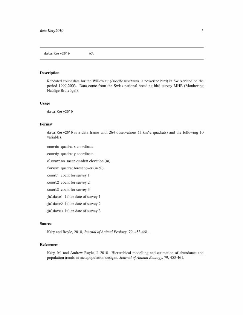
library(raster)library(sp)
#===================================#== Multivariate normal distributionrmvn <- function(n, mu = 0, V = matrix(1), seed=1234) {
p <- length(mu)if (any(is.na(match(dim(V), p)))) {
stop("Dimension problem!")}D <- chol(V)set.seed(seed)t(matrix(rnorm(n*p),ncol=p)%*%D+rep(mu,rep(n,p)))
}
#==================#== Data simulation
#= Set seed for repeatabilityseed <- 1234
#= LandscapexLand <- 30yLand <- 30Landscape <- raster(ncol=xLand,nrow=yLand,crs='+proj=utm +zone=1')Landscape[] <- 0extent(Landscape) <- c(0,xLand,0,yLand)coords <- coordinates(Landscape)ncells <- ncell(Landscape)
#= Neighborsneighbors.mat <- adjacent(Landscape, cells=c(1:ncells), directions=8, pairs=TRUE, sorted=TRUE)n.neighbors <- as.data.frame(table(as.factor(neighbors.mat[,1])))[,2]adj <- neighbors.mat[,2]
#= Generate symmetric adjacency matrix, AA <- matrix(0,ncells,ncells)index.start <- 1for (i in 1:ncells) {
index.end <- index.start+n.neighbors[i]-1A[i,adj[c(index.start:index.end)]] <- 1index.start <- index.end+1
}
#= Spatial effectsVrho.target <- 5d <- 1 # Spatial dependence parameter = 1 for intrinsic CARQ <- diag(n.neighbors)-d*A + diag(.0001,ncells) # Add small constant to make Q non-singularcovrho <- Vrho.target*solve(Q) # Covariance of rhosset.seed(seed)rho <- c(rmvn(1,mu=rep(0,ncells),V=covrho,seed=seed)) # Spatial Random Effectsrho <- rho-mean(rho) # Centering rhos on zero
hSDM.binomial.iCAR 15
#= Raster and plot spatial effectsr.rho <- rasterFromXYZ(cbind(coords,rho))plot(r.rho)
#= Sample the observation sites in the landscapensite <- 250set.seed(seed)x.coord <- runif(nsite,0,xLand)set.seed(2*seed)y.coord <- runif(nsite,0,yLand)sites.sp <- SpatialPoints(coords=cbind(x.coord,y.coord))cells <- extract(Landscape,sites.sp,cell=TRUE)[,1]
#= Number of visits associated to each observation pointset.seed(seed)visits <- rpois(nsite,3)visits[visits==0] <- 1
#= Ecological process (suitability)set.seed(seed)x1 <- rnorm(nsite,0,1)set.seed(2*seed)x2 <- rnorm(nsite,0,1)X <- cbind(rep(1,nsite),x1,x2)beta.target <- c(-1,1,-1)logit.theta <- X %*% beta.target + rho[cells]theta <- inv.logit(logit.theta)set.seed(seed)Y <- rbinom(nsite,visits,theta)
#= Relative importance of spatial random effectsRImp <- mean(abs(rho[cells])/abs(X %*% beta.target))RImp
#= Data-setsdata.obs <- data.frame(Y,visits,x1,x2,cell=cells)
#==================================#== Site-occupancy model
Start <- Sys.time() # Start the clockmod.hSDM.binomial.iCAR <- hSDM.binomial.iCAR(presences=data.obs$Y,
trials=data.obs$visits,suitability=~x1+x2,spatial.entity=data.obs$cell,data=data.obs,n.neighbors=n.neighbors,neighbors=adj,suitability.pred=NULL,spatial.entity.pred=NULL,burnin=5000, mcmc=5000, thin=5,beta.start=0,Vrho.start=1,

16 hSDM.binomial.iCAR
mubeta=0, Vbeta=1.0E6,priorVrho="1/Gamma",shape=0.5, rate=0.0005,seed=1234, verbose=1,save.rho=1, save.p=0)
Time.hSDM <- difftime(Sys.time(),Start,units="sec") # Time difference
#= Computation timeTime.hSDM
#==========#== Outputs
#= Parameter estimatessummary(mod.hSDM.binomial.iCAR$mcmc)pdf("Posteriors_hSDM.binomial.iCAR.pdf")plot(mod.hSDM.binomial.iCAR$mcmc)dev.off()
#= Predictionssummary(mod.hSDM.binomial.iCAR$theta.latent)summary(mod.hSDM.binomial.iCAR$theta.pred)pdf(file="Pred-Init.pdf")plot(theta,mod.hSDM.binomial.iCAR$theta.pred)abline(a=0,b=1,col="red")dev.off()
#= Summary plots for spatial random effects
# rho.predrho.pred <- apply(mod.hSDM.binomial.iCAR$rho.pred,2,mean)r.rho.pred <- rasterFromXYZ(cbind(coords,rho.pred))
# plotpdf(file="Summary_hSDM.binomial.iCAR.pdf")par(mfrow=c(2,2))# rho targetplot(r.rho, main="rho target")plot(sites.sp,add=TRUE)# rho estimatedplot(r.rho.pred, main="rho estimated")# correlation and "shrinkage"Levels.cells <- sort(unique(cells))plot(rho[-Levels.cells],rho.pred[-Levels.cells],
xlim=range(rho),ylim=range(rho),xlab="rho target",ylab="rho estimated")
points(rho[Levels.cells],rho.pred[Levels.cells],pch=16,col="blue")legend(x=-3,y=4,legend="Visited cells",col="blue",pch=16,bty="n")abline(a=0,b=1,col="red")dev.off()
hSDM.Nmixture 17
## End(Not run)
hSDM.Nmixture N-mixture model
Description
The hSDM.Nmixture function can be used to model species distribution including different pro-cesses in a hierarchical Bayesian framework: a Poisson suitability process (refering to environ-mental suitability explaining abundance) and a Binomial observability process (refering to variousecological and methodological issues explaining species detection). The hSDM.Nmixture functioncalls a Gibbs sampler written in C code which uses an adaptive Metropolis algorithm to estimatethe conditional posterior distribution of hierarchical model’s parameters.
Usage
hSDM.Nmixture(# Observationscounts, observability, site, data.observability,# Habitatsuitability, data.suitability,# Predictionssuitability.pred = NULL,# Chainsburnin = 5000, mcmc = 10000, thin = 10,# Starting valuesbeta.start,gamma.start,# Priorsmubeta = 0, Vbeta = 1.0E6,mugamma = 0, Vgamma = 1.0E6,# Variousseed = 1234, verbose = 1,save.p = 0, save.N = 0)
Arguments
counts A vector indicating the count (or abundance) for each observation.
observability A one-sided formula of the form ∼ w1 + ... + wq with q terms specifying theexplicative variables for the observability process.
site A vector indicating the site identifier (from one to the total number of sites) foreach observation. Several observations can occur at one site. A site can be araster cell for example.
data.observability
A data frame containing the model’s variables for the observability process.

18 hSDM.Nmixture
suitability A one-sided formula of the form ∼ x1 + ... + xp with p terms specifying theexplicative variables for the suitability process.
data.suitability
A data frame containing the model’s variables for the suitability process.suitability.pred
An optional data frame in which to look for variables with which to predict. IfNULL, the observations are used.
burnin The number of burnin iterations for the sampler.
mcmc The number of Gibbs iterations for the sampler. Total number of Gibbs iterationsis equal to burnin+mcmc. burnin+mcmc must be divisible by 10 and superior orequal to 100 so that the progress bar can be displayed.
thin The thinning interval used in the simulation. The number of mcmc iterationsmust be divisible by this value.
beta.start Starting values for β parameters of the suitability process. This can either be ascalar or a p-length vector.
gamma.start Starting values for β parameters of the observability process. This can either bea scalar or a q-length vector.
mubeta Means of the priors for the β parameters of the suitability process. mubeta mustbe either a scalar or a p-length vector. If mubeta takes a scalar value, then thatvalue will serve as the prior mean for all of the betas. The default value is set to0 for an uninformative prior.
Vbeta Variances of the Normal priors for the β parameters of the suitability process.Vbeta must be either a scalar or a p-length vector. If Vbeta takes a scalar value,then that value will serve as the prior variance for all of the betas. The defaultvariance is large and set to 1.0E6 for an uninformative flat prior.
mugamma Means of the Normal priors for the γ parameters of the observability process.mugamma must be either a scalar or a p-length vector. If mugamma takes a scalarvalue, then that value will serve as the prior mean for all of the gammas. Thedefault value is set to 0 for an uninformative prior.
Vgamma Variances of the Normal priors for the γ parameters of the observability process.Vgamma must be either a scalar or a p-length vector. If Vgamma takes a scalarvalue, then that value will serve as the prior variance for all of the gammas. Thedefault variance is large and set to 1.0E6 for an uninformative flat prior.
seed The seed for the random number generator. Default set to 1234.
verbose A switch (0,1) which determines whether or not the progress of the sampler isprinted to the screen. Default is 1: a progress bar is printed, indicating the step(in %) reached by the Gibbs sampler.
save.p A switch (0,1) which determines whether or not the sampled values for predic-tions are saved. Default is 0: the posterior mean is computed and returned inthe lambda.pred vector. Be careful, setting save.p to 1 might require a largeamount of memory.
save.N A switch (0,1) which determines whether or not the sampled values for the latentcount variable N for each observed cells are saved. Default is 0: the mean(rounded to the closest integer) is computed and returned in the N.pred vector.Be careful, setting save.N to 1 might require a large amount of memory.

hSDM.Nmixture 19
Details
The model integrates two processes, an ecological process associated to the abundance of thespecies due to habitat suitability and an observation process that takes into account the fact thatthe probability of detection of the species is inferior to one.
Ecological process:Ni ∼ Poisson(λi)
log(λi) = Xiβ
Observation process:yit ∼ Binomial(Ni, δit)
logit(δit) =Witγ
Value
mcmc An mcmc object that contains the posterior sample. This object can be summa-rized by functions provided by the coda package. The posterior sample of thedeviance D, with D = −2 log(
∏it P (yit, Ni|...)), is also provided.
lambda.pred If save.p is set to 0 (default), lambda.pred is the predictive posterior meanof the abundance associated to the suitability process for each prediction. Ifsave.p is set to 1, lambda.pred is an mcmc object with sampled values of theabundance associated to the suitability process for each prediction.
N.pred If save.N is set to 0 (default), N.pred is the posterior mean (rounded to theclosest integer) of the latent count variable N for each observed cell. If save.Nis set to 1, N.pred is an mcmc object with sampled values of the latent countvariable N for each observed cell.
lambda.latent Predictive posterior mean of the abundance associated to the suitability processfor each observation.
delta.latent Predictive posterior mean of the probability associated to the observability pro-cess for each observation.
Author(s)
Ghislain Vieilledent <[email protected]>
References
Gelfand, A. E.; Schmidt, A. M.; Wu, S.; Silander, J. A.; Latimer, A. and Rebelo, A. G. (2005)Modelling species diversity through species level hierarchical modelling. Applied Statistics, 54,1-20.
Latimer, A. M.; Wu, S. S.; Gelfand, A. E. and Silander, J. A. (2006) Building statistical models toanalyze species distributions. Ecological Applications, 16, 33-50.
Royle, J. A. (2004) N-mixture models for estimating population size from spatially replicatedcounts. Biometrics, 60, 108-115.
20 hSDM.Nmixture
See Also
plot.mcmc, summary.mcmc
Examples
## Not run:
#==============================================# hSDM.Nmixture()# Example with simulated data#==============================================
#=================#== Load librarieslibrary(hSDM)
#==================#== Data simulation
# Number of observation sitesnsite <- 200
#= Set seed for repeatabilityseed <- 4321
#= Ecological process (suitability)set.seed(seed)x1 <- rnorm(nsite,0,1)set.seed(2*seed)x2 <- rnorm(nsite,0,1)X <- cbind(rep(1,nsite),x1,x2)beta.target <- c(-1,1,-1) # Target parameterslog.lambda <- X %*% beta.targetlambda <- exp(log.lambda)set.seed(seed)N <- rpois(nsite,lambda)
#= Number of visits associated to each observation pointset.seed(seed)visits <- rpois(nsite,3)visits[visits==0] <- 1# Vector of observation pointssites <- vector()for (i in 1:nsite) {
sites <- c(sites,rep(i,visits[i]))}
#= Observation process (detectability)nobs <- sum(visits)set.seed(seed)w1 <- rnorm(nobs,0,1)

hSDM.Nmixture 21
set.seed(2*seed)w2 <- rnorm(nobs,0,1)W <- cbind(rep(1,nobs),w1,w2)gamma.target <- c(-1,1,-1) # Target parameterslogit.delta <- W %*% gamma.targetdelta <- inv.logit(logit.delta)set.seed(seed)Y <- rbinom(nobs,N[sites],delta)
#= Data-setsdata.obs <- data.frame(Y,w1,w2,site=sites)data.suit <- data.frame(x1,x2)
#================================#== Parameter inference with hSDM
Start <- Sys.time() # Start the clockmod.hSDM.Nmixture <- hSDM.Nmixture(# Observations
counts=data.obs$Y,observability=~w1+w2,site=data.obs$site,data.observability=data.obs,# Habitatsuitability=~x1+x2,data.suitability=data.suit,# Predictionssuitability.pred=NULL,# Chainsburnin=5000, mcmc=5000, thin=5,# Starting valuesbeta.start=0,gamma.start=0,# Priorsmubeta=0, Vbeta=1.0E6,mugamma=0, Vgamma=1.0E6,# Variousseed=1234, verbose=1,save.p=0, save.N=1)
Time.hSDM <- difftime(Sys.time(),Start,units="sec") # Time difference
#= Computation timeTime.hSDM
#==========#== Outputs
#= Parameter estimatessummary(mod.hSDM.Nmixture$mcmc)pdf(file="Posteriors_hSDM.Nmixture.pdf")plot(mod.hSDM.Nmixture$mcmc)dev.off()
#= Predictions

22 hSDM.Nmixture.iCAR
summary(mod.hSDM.Nmixture$lambda.latent)summary(mod.hSDM.Nmixture$delta.latent)summary(mod.hSDM.Nmixture$lambda.pred)pdf(file="Pred-Init.pdf")plot(lambda,mod.hSDM.Nmixture$lambda.pred)abline(a=0,b=1,col="red")dev.off()
#= MCMC for latent variable Npdf(file="MCMC_N.pdf")plot(mod.hSDM.Nmixture$N.pred)dev.off()
#= Check that Ns are correctly estimatedM <- as.matrix(mod.hSDM.Nmixture$N.pred)N.est <- apply(M,2,mean)Y.by.site <- tapply(data.obs$Y,data.obs$site,mean) # Mean by sitepdf(file="Check_N.pdf",width=10,height=5)par(mfrow=c(1,2))plot(Y.by.site, N.est) ## More individuals are expected (N > Y) due to detection processabline(a=0,b=1,col="red")plot(N, N.est) ## N are well estimatedabline(a=0,b=1,col="red")cor(N, N.est) ## Very close to 1dev.off()
## End(Not run)
hSDM.Nmixture.iCAR N-mixture model with CAR process
Description
The hSDM.Nmixture.iCAR function can be used to model species distribution including differentprocesses in a hierarchical Bayesian framework: a Poisson suitability process (refering to envi-ronmental suitability explaining abundance) which takes into account the spatial dependence of theobservations, and a Binomial observability process (refering to various ecological and method-ological issues explaining the species detection). The hSDM.Nmixture.iCAR function calls a Gibbssampler written in C code which uses an adaptive Metropolis algorithm to estimate the conditionalposterior distribution of hierarchical model’s parameters.
Usage
hSDM.Nmixture.iCAR(# Observationscounts, observability, site, data.observability,# Habitatsuitability, data.suitability,

hSDM.Nmixture.iCAR 23
# Spatial structurespatial.entity,n.neighbors, neighbors,# Predictionssuitability.pred = NULL, spatial.entity.pred = NULL,# Chainsburnin = 5000, mcmc = 10000, thin = 10,# Starting valuesbeta.start,gamma.start,Vrho.start,# Priorsmubeta = 0, Vbeta = 1.0E6,mugamma = 0, Vgamma = 1.0E6,priorVrho = "1/Gamma",shape = 0.5, rate = 0.0005,Vrho.max = 1000,# Variousseed = 1234, verbose = 1,save.rho = 0, save.p = 0, save.N = 0)
Arguments
counts A vector indicating the count (or abundance) for each observation.
observability A one-sided formula of the form ∼ w1 + ... + wq with q terms specifying theexplicative variables for the observability process.
site A vector indicating the site identifier (from one to the total number of sites) foreach observation. Several observations can occur at one site. A site can be araster cell for example.
data.observability
A data frame containing the model’s variables for the observability process.
suitability A one-sided formula of the form ∼ x1 + ... + xp with p terms specifying theexplicative variables for the suitability process.
data.suitability
A data frame containing the model’s variables for the suitability process. Thenumber of rows of the data frame should be equal to the total number of spatialentities.
spatial.entity A vector (of length ’nsite’) indicating the spatial entity identifier for each site.Values must be between 1 and the total number of spatial entities. Several sitescan be found in one spatial entity. A spatial entity can be a raster cell for exam-ple.
n.neighbors A vector of integers that indicates the number of neighbors (adjacent entities) ofeach spatial entity. length(n.neighbors) indicates the total number of spatialentities.
neighbors A vector of integers indicating the neighbors (adjacent entities) of each spatialentity. Must be of the form c(neighbors of entity 1, neighbors of entity 2, ... ,

24 hSDM.Nmixture.iCAR
neighbors of the last entity). Length of the neighbors vector should be equal tosum(n.neighbors).
suitability.pred
An optional data frame in which to look for variables with which to predict. IfNULL, the data frame data.suitability for observations is used.
spatial.entity.pred
An optional vector indicating the spatial entity identifier (from one to the totalnumber of entities) for predictions. If NULL, the vector spatial.entity forobservations is used.
burnin The number of burnin iterations for the sampler.
mcmc The number of Gibbs iterations for the sampler. Total number of Gibbs iterationsis equal to burnin+mcmc. burnin+mcmc must be divisible by 10 and superior orequal to 100 so that the progress bar can be displayed.
thin The thinning interval used in the simulation. The number of mcmc iterationsmust be divisible by this value.
beta.start Starting values for β parameters of the suitability process. This can either be ascalar or a p-length vector.
gamma.start Starting values for β parameters of the observability process. This can either bea scalar or a q-length vector.
Vrho.start Positive scalar indicating the starting value for the variance of the spatial randomeffects.
mubeta Means of the priors for the β parameters of the suitability process. mubeta mustbe either a scalar or a p-length vector. If mubeta takes a scalar value, then thatvalue will serve as the prior mean for all of the betas. The default value is set to0 for an uninformative prior.
Vbeta Variances of the Normal priors for the β parameters of the suitability process.Vbeta must be either a scalar or a p-length vector. If Vbeta takes a scalar value,then that value will serve as the prior variance for all of the betas. The defaultvariance is large and set to 1.0E6 for an uninformative flat prior.
mugamma Means of the Normal priors for the γ parameters of the observability process.mugamma must be either a scalar or a p-length vector. If mugamma takes a scalarvalue, then that value will serve as the prior mean for all of the gammas. Thedefault value is set to 0 for an uninformative prior.
Vgamma Variances of the Normal priors for the γ parameters of the observability process.Vgamma must be either a scalar or a p-length vector. If Vgamma takes a scalarvalue, then that value will serve as the prior variance for all of the gammas. Thedefault variance is large and set to 1.0E6 for an uninformative flat prior.
priorVrho Type of prior for the variance of the spatial random effects. Can be set to a fixedpositive scalar, or to an inverse-gamma distribution ("1/Gamma") with param-eters shape and rate, or to a uniform distribution ("Uniform") on the interval[0,Vrho.max]. Default set to "1/Gamma".
shape The shape parameter for the Gamma prior on the precision of the spatial randomeffects. Default value is shape=0.05 for uninformative prior.
rate The rate (1/scale) parameter for the Gamma prior on the precision of the spatialrandom effects. Default value is rate=0.0005 for uninformative prior.

hSDM.Nmixture.iCAR 25
Vrho.max Upper bound for the uniform prior of the spatial random effect variance. Defaultset to 1000.
seed The seed for the random number generator. Default set to 1234.
verbose A switch (0,1) which determines whether or not the progress of the sampler isprinted to the screen. Default is 1: a progress bar is printed, indicating the step(in %) reached by the Gibbs sampler.
save.rho A switch (0,1) which determines whether or not the sampled values for rhosare saved. Default is 0: the posterior mean is computed and returned in therho.pred vector. Be careful, setting save.rho to 1 might require a large amountof memory.
save.p A switch (0,1) which determines whether or not the sampled values for predic-tions are saved. Default is 0: the posterior mean is computed and returned inthe lambda.pred vector. Be careful, setting save.p to 1 might require a largeamount of memory.
save.N A switch (0,1) which determines whether or not the sampled values for the latentcount variable N for each observed cells are saved. Default is 0: the mean(rounded to the closest integer) is computed and returned in the N.pred vector.Be careful, setting save.N to 1 might require a large amount of memory.
Details
The model integrates two processes, an ecological process associated to the abundance of thespecies due to habitat suitability and an observation process that takes into account the fact thatthe probability of detection of the species is inferior to one. The ecological process includes anintrinsic conditional autoregressive model (iCAR) model for spatial autocorrelation between obser-vations, assuming that the abundance of the species at one site depends on the abundance of thespecies on neighboring sites.
Ecological process:Ni ∼ Poisson(λi)
log(λi) = Xiβ + ρi
ρi: spatial random effect
Spatial autocorrelation:
An intrinsic conditional autoregressive model (iCAR) is assumed:
ρi ∼ N ormal(µi, Vρ/ni)
µi: mean of ρi′ in the neighborhood of i.
Vρ: variance of the spatial random effects.
ni: number of neighbors for spatial entity i.
Observation process:yit ∼ Binomial(Ni, δit)
logit(δit) =Witγ

26 hSDM.Nmixture.iCAR
Value
mcmc An mcmc object that contains the posterior sample. This object can be summa-rized by functions provided by the coda package. The posterior sample of thedeviance D, with D = −2 log(
∏it P (yit, Ni|...)), is also provided.
rho.pred If save.rho is set to 0 (default), rho.pred is the predictive posterior mean ofthe spatial random effect associated to each spatial entity. If save.rho is setto 1, rho.pred is an mcmc object with sampled values for each spatial randomeffect associated to each spatial entity.
lambda.pred If save.p is set to 0 (default), lambda.pred is the predictive posterior meanof the abundance associated to the suitability process for each prediction. Ifsave.p is set to 1, lambda.pred is an mcmc object with sampled values of theabundance associated to the suitability process for each prediction.
N.pred If save.N is set to 0 (default), N.pred is the posterior mean (rounded to theclosest integer) of the latent count variable N for each observed cell. If save.Nis set to 1, N.pred is an mcmc object with sampled values of the latent countvariable N for each observed cell.
lambda.latent Predictive posterior mean of the abundance associated to the suitability processfor each observation.
delta.latent Predictive posterior mean of the probability associated to the observability pro-cess for each observation.
Author(s)
Ghislain Vieilledent <[email protected]>
References
Gelfand, A. E.; Schmidt, A. M.; Wu, S.; Silander, J. A.; Latimer, A. and Rebelo, A. G. (2005)Modelling species diversity through species level hierarchical modelling. Applied Statistics, 54,1-20.
Latimer, A. M.; Wu, S. S.; Gelfand, A. E. and Silander, J. A. (2006) Building statistical models toanalyze species distributions. Ecological Applications, 16, 33-50.
Royle, J. A. (2004) N-mixture models for estimating population size from spatially replicatedcounts. Biometrics, 60, 108-115.
See Also
plot.mcmc, summary.mcmc
Examples
## Not run:
#==============================================# hSDM.Nmixture.iCAR()# Example with simulated data

hSDM.Nmixture.iCAR 27
#==============================================
#=================#== Load librarieslibrary(hSDM)library(raster)library(sp)
#===================================#== Multivariate normal distributionrmvn <- function(n, mu = 0, V = matrix(1), seed=1234) {
p <- length(mu)if (any(is.na(match(dim(V), p)))) {
stop("Dimension problem!")}D <- chol(V)set.seed(seed)t(matrix(rnorm(n*p),ncol=p)%*%D+rep(mu,rep(n,p)))
}
#==================#== Data simulation
#= Set seed for repeatabilityseed <- 4321
#= LandscapexLand <- 20yLand <- 20Landscape <- raster(ncol=xLand,nrow=yLand,crs='+proj=utm +zone=1')Landscape[] <- 0extent(Landscape) <- c(0,xLand,0,yLand)coords <- coordinates(Landscape)ncells <- ncell(Landscape)
#= Neighborsneighbors.mat <- adjacent(Landscape, cells=c(1:ncells), directions=8, pairs=TRUE, sorted=TRUE)n.neighbors <- as.data.frame(table(as.factor(neighbors.mat[,1])))[,2]adj <- neighbors.mat[,2]
#= Generate symmetric adjacency matrix, AA <- matrix(0,ncells,ncells)index.start <- 1for (i in 1:ncells) {
index.end <- index.start+n.neighbors[i]-1A[i,adj[c(index.start:index.end)]] <- 1index.start <- index.end+1
}
#= Spatial effectsVrho.target <- 5d <- 1 # Spatial dependence parameter = 1 for intrinsic CAR

28 hSDM.Nmixture.iCAR
Q <- diag(n.neighbors)-d*A + diag(.0001,ncells) # Add small constant to make Q non-singularcovrho <- Vrho.target*solve(Q) # Covariance of rhosset.seed(seed)rho <- c(rmvn(1,mu=rep(0,ncells),V=covrho,seed=seed)) # Spatial Random Effectsrho <- rho-mean(rho) # Centering rhos on zero
#= Raster and plot spatial effectsr.rho <- rasterFromXYZ(cbind(coords,rho))plot(r.rho)
#= Sample the observation sites in the landscapensite <- 150set.seed(seed)x.coord <- runif(nsite,0,xLand)set.seed(2*seed)y.coord <- runif(nsite,0,yLand)sites.sp <- SpatialPoints(coords=cbind(x.coord,y.coord))cells <- extract(Landscape,sites.sp,cell=TRUE)[,1]
#= Ecological process (suitability)set.seed(seed)x1 <- rnorm(nsite,0,1)set.seed(2*seed)x2 <- rnorm(nsite,0,1)X <- cbind(rep(1,nsite),x1,x2)beta.target <- c(-1,1,-1)log.lambda <- X %*% beta.target + rho[cells]lambda <- exp(log.lambda)set.seed(seed)N <- rpois(nsite,lambda)
#= Relative importance of spatial random effectsRImp <- mean(abs(rho[cells])/abs(X %*% beta.target))RImp
#= Number of visits associated to each observation pointset.seed(seed)visits <- rpois(nsite,3)visits[visits==0] <- 1# Vector of observation pointssites <- vector()for (i in 1:nsite) {
sites <- c(sites,rep(i,visits[i]))}
#= Observation process (detectability)nobs <- sum(visits)set.seed(seed)w1 <- rnorm(nobs,0,1)set.seed(2*seed)w2 <- rnorm(nobs,0,1)W <- cbind(rep(1,nobs),w1,w2)gamma.target <- c(-1,1,-1)
hSDM.Nmixture.iCAR 29
logit.delta <- W %*% gamma.targetdelta <- inv.logit(logit.delta)set.seed(seed)Y <- rbinom(nobs,N[sites],delta)
#= Data-setsdata.obs <- data.frame(Y,w1,w2,site=sites)data.suit <- data.frame(x1,x2,cell=cells)
#================================#== Parameter inference with hSDM
Start <- Sys.time() # Start the clockmod.hSDM.Nmixture.iCAR <- hSDM.Nmixture.iCAR(# Observations
counts=data.obs$Y,observability=~w1+w2,site=data.obs$site,data.observability=data.obs,# Habitatsuitability=~x1+x2, data.suitability=data.suit,# Spatial structurespatial.entity=data.suit$cell,n.neighbors=n.neighbors, neighbors=adj,# Predictionssuitability.pred=NULL,spatial.entity.pred=NULL,# Chainsburnin=5000, mcmc=5000, thin=5,# Starting valuesbeta.start=0,gamma.start=0,Vrho.start=1,# Priorsmubeta=0, Vbeta=1.0E6,mugamma=0, Vgamma=1.0E6,priorVrho="1/Gamma",shape=0.5, rate=0.005,Vrho.max=10,# Variousseed=1234, verbose=1,save.rho=1, save.p=0, save.N=1)
Time.hSDM <- difftime(Sys.time(),Start,units="sec") # Time difference
#= Computation timeTime.hSDM
#==========#== Outputs
#= Parameter estimatessummary(mod.hSDM.Nmixture.iCAR$mcmc)pdf(file="Posteriors_hSDM.Nmixture.iCAR.pdf")plot(mod.hSDM.Nmixture.iCAR$mcmc)

30 hSDM.Nmixture.iCAR
dev.off()
#= Predictionssummary(mod.hSDM.Nmixture.iCAR$lambda.latent)summary(mod.hSDM.Nmixture.iCAR$delta.latent)summary(mod.hSDM.Nmixture.iCAR$lambda.pred)pdf(file="Pred-Init.pdf")plot(lambda,mod.hSDM.Nmixture.iCAR$lambda.pred)abline(a=0,b=1,col="red")dev.off()
#= MCMC for latent variable Npdf(file="MCMC_N.pdf")plot(mod.hSDM.Nmixture.iCAR$N.pred)dev.off()
#= Check that Ns are corretly estimatedM <- as.matrix(mod.hSDM.Nmixture.iCAR$N.pred)N.est <- apply(M,2,mean)Y.by.site <- tapply(data.obs$Y,data.obs$site,mean) # Mean by sitepdf(file="Check_N.pdf",width=10,height=5)par(mfrow=c(1,2))plot(Y.by.site, N.est) ## More individuals are expected (N > Y) due to detection processabline(a=0,b=1,col="red")plot(N, N.est) ## N are well estimatedabline(a=0,b=1,col="red")cor(N, N.est) ## Very close to 1dev.off()
#= Summary plots for spatial random effects
# rho.predrho.pred <- apply(mod.hSDM.Nmixture.iCAR$rho.pred,2,mean)r.rho.pred <- rasterFromXYZ(cbind(coords,rho.pred))
# plotpdf(file="Summary_hSDM.Nmixture.iCAR.pdf")par(mfrow=c(2,2))# rho targetplot(r.rho, main="rho target")plot(sites.sp,add=TRUE)# rho estimatedplot(r.rho.pred, main="rho estimated")# correlation and "shrinkage"Levels.cells <- sort(unique(cells))plot(rho[-Levels.cells],rho.pred[-Levels.cells],
xlim=range(rho),ylim=range(rho),xlab="rho target",ylab="rho estimated")
points(rho[Levels.cells],rho.pred[Levels.cells],pch=16,col="blue")legend(x=-3,y=4,legend="Visited cells",col="blue",pch=16,bty="n")abline(a=0,b=1,col="red")

hSDM.poisson 31
dev.off()
## End(Not run)
hSDM.poisson Poisson log regression model
Description
The hSDM.poisson function performs a Poisson log regression in a Bayesian framework. Thefunction calls a Gibbs sampler written in C code which uses an adaptive Metropolis algorithm toestimate the conditional posterior distribution of model’s parameters.
Usage
hSDM.poisson(counts, suitability, data, suitability.pred = NULL,burnin = 5000, mcmc = 10000, thin = 10, beta.start, mubeta = 0, Vbeta =1e+06, seed = 1234, verbose = 1, save.p = 0)
Arguments
counts A vector indicating the count (or abundance) for each observation.
suitability A one-sided formula of the form ’~x1+...+xp’ with p terms specifying the ex-plicative covariates for the suitability process of the model.
data A data frame containing the model’s explicative variables.suitability.pred
An optional data frame in which to look for variables with which to predict. IfNULL, the observations are used.
burnin The number of burnin iterations for the sampler.
mcmc The number of Gibbs iterations for the sampler. Total number of Gibbs iterationsis equal to burnin+mcmc. burnin+mcmc must be divisible by 10 and superior orequal to 100 so that the progress bar can be displayed.
thin The thinning interval used in the simulation. The number of mcmc iterationsmust be divisible by this value.
beta.start Starting values for beta parameters of the suitability process. If beta.starttakes a scalar value, then that value will serve for all of the betas.
mubeta Means of the priors for the β parameters of the suitability process. mubeta mustbe either a scalar or a p-length vector. If mubeta takes a scalar value, then thatvalue will serve as the prior mean for all of the betas. The default value is set to0 for an uninformative prior.
Vbeta Variances of the Normal priors for the β parameters of the suitability process.Vbeta must be either a scalar or a p-length vector. If Vbeta takes a scalar value,then that value will serve as the prior variance for all of the betas. The defaultvariance is large and set to 1.0E6 for an uninformative flat prior.

32 hSDM.poisson
seed The seed for the random number generator. Default to 1234.
verbose A switch (0,1) which determines whether or not the progress of the sampler isprinted to the screen. Default is 1: a progress bar is printed, indicating the step(in %) reached by the Gibbs sampler.
save.p A switch (0,1) which determines whether or not the sampled values for predic-tions are saved. Default is 0: the posterior mean is computed and returned inthe lambda.pred vector. Be careful, setting save.p to 1 might require a largeamount of memory.
Details
We model the abundance of the species as a function of environmental variables.
Ecological process:yi ∼ Poisson(λi)
log(λi) = Xiβ
Value
mcmc An mcmc object that contains the posterior sample. This object can be summa-rized by functions provided by the coda package. The posterior sample of thedeviance D, with D = −2 log(
∏i P (yi, ni|β)), is also provided.
lambda.pred If save.p is set to 0 (default), lambda.pred is the predictive posterior meanof the abundance associated to the suitability process for each prediction. Ifsave.p is set to 1, lambda.pred is an mcmc object with sampled values of theabundance associated to the suitability process for each prediction.
lambda.latent Predictive posterior mean of the abundance associated to the suitability processfor each observation.
Author(s)
Ghislain Vieilledent <[email protected]>
References
Latimer, A. M.; Wu, S. S.; Gelfand, A. E. and Silander, J. A. (2006) Building statistical models toanalyze species distributions. Ecological Applications, 16, 33-50.
Gelfand, A. E.; Schmidt, A. M.; Wu, S.; Silander, J. A.; Latimer, A. and Rebelo, A. G. (2005)Modelling species diversity through species level hierarchical modelling. Applied Statistics, 54,1-20.
See Also
plot.mcmc, summary.mcmc
hSDM.poisson 33
Examples
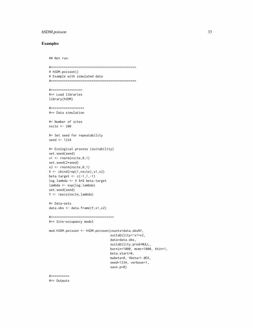
## Not run:
#==============================================# hSDM.poisson()# Example with simulated data#==============================================
#=================#== Load librarieslibrary(hSDM)
#==================#== Data simulation
#= Number of sitesnsite <- 200
#= Set seed for repeatabilityseed <- 1234
#= Ecological process (suitability)set.seed(seed)x1 <- rnorm(nsite,0,1)set.seed(2*seed)x2 <- rnorm(nsite,0,1)X <- cbind(rep(1,nsite),x1,x2)beta.target <- c(-1,1,-1)log.lambda <- X %*% beta.targetlambda <- exp(log.lambda)set.seed(seed)Y <- rpois(nsite,lambda)
#= Data-setsdata.obs <- data.frame(Y,x1,x2)
#==================================#== Site-occupancy model
mod.hSDM.poisson <- hSDM.poisson(counts=data.obs$Y,suitability=~x1+x2,data=data.obs,suitability.pred=NULL,burnin=1000, mcmc=1000, thin=1,beta.start=0,mubeta=0, Vbeta=1.0E6,seed=1234, verbose=1,save.p=0)
#==========#== Outputs
34 hSDM.poisson.iCAR
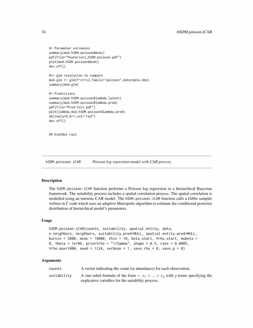
#= Parameter estimatessummary(mod.hSDM.poisson$mcmc)pdf(file="Posteriors_hSDM.poisson.pdf")plot(mod.hSDM.poisson$mcmc)dev.off()
#== glm resolution to comparemod.glm <- glm(Y~x1+x2,family="poisson",data=data.obs)summary(mod.glm)
#= Predictionssummary(mod.hSDM.poisson$lambda.latent)summary(mod.hSDM.poisson$lambda.pred)pdf(file="Pred-Init.pdf")plot(lambda,mod.hSDM.poisson$lambda.pred)abline(a=0,b=1,col="red")dev.off()
## End(Not run)
hSDM.poisson.iCAR Poisson log regression model with CAR process
Description
The hSDM.poisson.iCAR function performs a Poisson log regression in a hierarchical Bayesianframework. The suitability process includes a spatial correlation process. The spatial correlation ismodelled using an intrinsic CAR model. The hSDM.poisson.iCAR function calls a Gibbs samplerwritten in C code which uses an adaptive Metropolis algorithm to estimate the conditional posteriordistribution of hierarchical model’s parameters.
Usage
hSDM.poisson.iCAR(counts, suitability, spatial.entity, data,n.neighbors, neighbors, suitability.pred=NULL, spatial.entity.pred=NULL,burnin = 5000, mcmc = 10000, thin = 10, beta.start, Vrho.start, mubeta =0, Vbeta = 1e+06, priorVrho = "1/Gamma", shape = 0.5, rate = 0.0005,Vrho.max=1000, seed = 1234, verbose = 1, save.rho = 0, save.p = 0)
Arguments
counts A vector indicating the count (or abundance) for each observation.
suitability A one-sided formula of the form ∼ x1 + ... + xp with p terms specifying theexplicative variables for the suitability process.

hSDM.poisson.iCAR 35
spatial.entity A vector indicating the spatial entity identifier (from one to the total numberof entities) for each observation. Several observations can occur in one spatialentity. A spatial entity can be a raster cell for example.
data A data frame containing the model’s variables.
n.neighbors A vector of integers that indicates the number of neighbors (adjacent entities) ofeach spatial entity. length(n.neighbors) indicates the total number of spatialentities.
neighbors A vector of integers indicating the neighbors (adjacent entities) of each spatialentity. Must be of the form c(neighbors of entity 1, neighbors of entity 2, ... ,neighbors of the last entity). Length of the neighbors vector should be equal tosum(n.neighbors).
suitability.pred
An optional data frame in which to look for variables with which to predict. IfNULL, the observations are used.
spatial.entity.pred
An optional vector indicating the spatial entity identifier (from one to the totalnumber of entities) for predictions. If NULL, the vector spatial.entity forobservations is used.
burnin The number of burnin iterations for the sampler.
mcmc The number of Gibbs iterations for the sampler. Total number of Gibbs iterationsis equal to burnin+mcmc. burnin+mcmc must be divisible by 10 and superior orequal to 100 so that the progress bar can be displayed.
thin The thinning interval used in the simulation. The number of mcmc iterationsmust be divisible by this value.
beta.start Starting values for β parameters of the suitability process. This can either be ascalar or a p-length vector.
Vrho.start Positive scalar indicating the starting value for the variance of the spatial randomeffects.
mubeta Means of the priors for the β parameters of the suitability process. mubeta mustbe either a scalar or a p-length vector. If mubeta takes a scalar value, then thatvalue will serve as the prior mean for all of the betas. The default value is set to0 for an uninformative prior.
Vbeta Variances of the Normal priors for the β parameters of the suitability process.Vbeta must be either a scalar or a p-length vector. If Vbeta takes a scalar value,then that value will serve as the prior variance for all of the betas. The defaultvariance is large and set to 1.0E6 for an uninformative flat prior.
priorVrho Type of prior for the variance of the spatial random effects. Can be set to a fixedpositive scalar, or to an inverse-gamma distribution ("1/Gamma") with param-eters shape and rate, or to a uniform distribution ("Uniform") on the interval[0,Vrho.max]. Default set to "1/Gamma".
shape The shape parameter for the Gamma prior on the precision of the spatial randomeffects. Default value is shape=0.05 for uninformative prior.
rate The rate (1/scale) parameter for the Gamma prior on the precision of the spatialrandom effects. Default value is rate=0.0005 for uninformative prior.
36 hSDM.poisson.iCAR
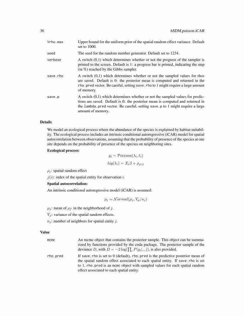
Vrho.max Upper bound for the uniform prior of the spatial random effect variance. Defaultset to 1000.
seed The seed for the random number generator. Default set to 1234.
verbose A switch (0,1) which determines whether or not the progress of the sampler isprinted to the screen. Default is 1: a progress bar is printed, indicating the step(in %) reached by the Gibbs sampler.
save.rho A switch (0,1) which determines whether or not the sampled values for rhosare saved. Default is 0: the posterior mean is computed and returned in therho.pred vector. Be careful, setting save.rho to 1 might require a large amountof memory.
save.p A switch (0,1) which determines whether or not the sampled values for predic-tions are saved. Default is 0: the posterior mean is computed and returned inthe lambda.pred vector. Be careful, setting save.p to 1 might require a largeamount of memory.
Details
We model an ecological process where the abundance of the species is explained by habitat suitabil-ity. The ecological process includes an intrinsic conditional autoregressive (iCAR) model for spatialautocorrelation between observations, assuming that the probability of presence of the species at onesite depends on the probability of presence of the species on neighboring sites.
Ecological process:yi ∼ Poisson(λi, ti)
log(λi) = Xiβ + ρj(i)
ρj : spatial random effect
j(i): index of the spatial entity for observation i.
Spatial autocorrelation:
An intrinsic conditional autoregressive model (iCAR) is assumed:
ρj ∼ N ormal(µj , Vρ/nj)
µj : mean of ρj′ in the neighborhood of j.
Vρ: variance of the spatial random effects.
nj : number of neighbors for spatial entity j.
Value
mcmc An mcmc object that contains the posterior sample. This object can be summa-rized by functions provided by the coda package. The posterior sample of thedeviance D, with D = −2 log(
∏i P (yi|...)), is also provided.
rho.pred If save.rho is set to 0 (default), rho.pred is the predictive posterior mean ofthe spatial random effect associated to each spatial entity. If save.rho is setto 1, rho.pred is an mcmc object with sampled values for each spatial randomeffect associated to each spatial entity.

hSDM.poisson.iCAR 37
lambda.pred If save.p is set to 0 (default), lambda.pred is the predictive posterior meanof the abundance associated to the suitability process for each prediction. Ifsave.p is set to 1, lambda.pred is an mcmc object with sampled values of theabundance associated to the suitability process for each prediction.
lambda.latent Predictive posterior mean of the abundance associated to the suitability processfor each observation.
Author(s)
Ghislain Vieilledent <[email protected]>
References
Gelfand, A. E.; Schmidt, A. M.; Wu, S.; Silander, J. A.; Latimer, A. and Rebelo, A. G. (2005)Modelling species diversity through species level hierarchical modelling. Applied Statistics, 54,1-20.
Latimer, A. M.; Wu, S. S.; Gelfand, A. E. and Silander, J. A. (2006) Building statistical models toanalyze species distributions. Ecological Applications, 16, 33-50.
Lichstein, J. W.; Simons, T. R.; Shriner, S. A. & Franzreb, K. E. (2002) Spatial autocorrelation andautoregressive models in ecology Ecological Monographs, 72, 445-463.
Diez, J. M. & Pulliam, H. R. (2007) Hierarchical analysis of species distributions and abundanceacross environmental gradients Ecology, 88, 3144-3152.
See Also
plot.mcmc, summary.mcmc
Examples
## Not run:
#==============================================# hSDM.poisson.iCAR()# Example with simulated data#==============================================
#=================#== Load librarieslibrary(hSDM)library(raster)library(sp)
#===================================#== Multivariate normal distributionrmvn <- function(n, mu = 0, V = matrix(1), seed=1234) {
p <- length(mu)if (any(is.na(match(dim(V), p)))) {
stop("Dimension problem!")}

38 hSDM.poisson.iCAR
D <- chol(V)set.seed(seed)t(matrix(rnorm(n*p),ncol=p)%*%D+rep(mu,rep(n,p)))
}
#==================#== Data simulation
#= Set seed for repeatabilityseed <- 1234
#= LandscapexLand <- 30yLand <- 30Landscape <- raster(ncol=xLand,nrow=yLand,crs='+proj=utm +zone=1')Landscape[] <- 0extent(Landscape) <- c(0,xLand,0,yLand)coords <- coordinates(Landscape)ncells <- ncell(Landscape)
#= Neighborsneighbors.mat <- adjacent(Landscape, cells=c(1:ncells), directions=8, pairs=TRUE, sorted=TRUE)n.neighbors <- as.data.frame(table(as.factor(neighbors.mat[,1])))[,2]adj <- neighbors.mat[,2]
#= Generate symmetric adjacency matrix, AA <- matrix(0,ncells,ncells)index.start <- 1for (i in 1:ncells) {
index.end <- index.start+n.neighbors[i]-1A[i,adj[c(index.start:index.end)]] <- 1index.start <- index.end+1
}
#= Spatial effectsVrho.target <- 5d <- 1 # Spatial dependence parameter = 1 for intrinsic CARQ <- diag(n.neighbors)-d*A + diag(.0001,ncells) # Add small constant to make Q non-singularcovrho <- Vrho.target*solve(Q) # Covariance of rhosset.seed(seed)rho <- c(rmvn(1,mu=rep(0,ncells),V=covrho,seed=seed)) # Spatial Random Effectsrho <- rho-mean(rho) # Centering rhos on zero
#= Raster and plot spatial effectsr.rho <- rasterFromXYZ(cbind(coords,rho))plot(r.rho)
#= Sample the observation sites in the landscapensite <- 250set.seed(seed)x.coord <- runif(nsite,0,xLand)set.seed(2*seed)y.coord <- runif(nsite,0,yLand)

hSDM.poisson.iCAR 39
sites.sp <- SpatialPoints(coords=cbind(x.coord,y.coord))cells <- extract(Landscape,sites.sp,cell=TRUE)[,1]
#= Ecological process (suitability)set.seed(seed)x1 <- rnorm(nsite,0,1)set.seed(2*seed)x2 <- rnorm(nsite,0,1)X <- cbind(rep(1,nsite),x1,x2)beta.target <- c(-1,1,-1)log.lambda <- X %*% beta.target + rho[cells]lambda <- exp(log.lambda)set.seed(seed)Y <- rpois(nsite,lambda)
#= Relative importance of spatial random effectsRImp <- mean(abs(rho[cells])/abs(X %*% beta.target))RImp
#= Data-setsdata.obs <- data.frame(Y,x1,x2,cell=cells)
#==================================#== Site-occupancy model
Start <- Sys.time() # Start the clockmod.hSDM.poisson.iCAR <- hSDM.poisson.iCAR(counts=data.obs$Y,
suitability=~x1+x2,spatial.entity=data.obs$cell,data=data.obs,n.neighbors=n.neighbors,neighbors=adj,suitability.pred=NULL,spatial.entity.pred=NULL,burnin=5000, mcmc=5000, thin=5,beta.start=0,Vrho.start=1,mubeta=0, Vbeta=1.0E6,priorVrho="1/Gamma",shape=0.5, rate=0.0005,seed=1234, verbose=1,save.rho=1, save.p=0)
Time.hSDM <- difftime(Sys.time(),Start,units="sec") # Time difference
#= Computation timeTime.hSDM
#==========#== Outputs
#= Parameter estimatessummary(mod.hSDM.poisson.iCAR$mcmc)pdf("Posteriors_hSDM.poisson.iCAR.pdf")

40 hSDM.siteocc
plot(mod.hSDM.poisson.iCAR$mcmc)dev.off()
#= Predictionssummary(mod.hSDM.poisson.iCAR$lambda.latent)summary(mod.hSDM.poisson.iCAR$lambda.pred)pdf(file="Pred-Init.pdf")plot(lambda,mod.hSDM.poisson.iCAR$lambda.pred)abline(a=0,b=1,col="red")dev.off()
#= Summary plots for spatial random effects
# rho.predrho.pred <- apply(mod.hSDM.poisson.iCAR$rho.pred,2,mean)r.rho.pred <- rasterFromXYZ(cbind(coords,rho.pred))
# plotpdf(file="Summary_hSDM.poisson.iCAR.pdf")par(mfrow=c(2,2))# rho targetplot(r.rho, main="rho target")plot(sites.sp,add=TRUE)# rho estimatedplot(r.rho.pred, main="rho estimated")# correlation and "shrinkage"Levels.cells <- sort(unique(cells))plot(rho[-Levels.cells],rho.pred[-Levels.cells],
xlim=range(rho),ylim=range(rho),xlab="rho target",ylab="rho estimated")
points(rho[Levels.cells],rho.pred[Levels.cells],pch=16,col="blue")legend(x=-3,y=4,legend="Visited cells",col="blue",pch=16,bty="n")abline(a=0,b=1,col="red")dev.off()
## End(Not run)
hSDM.siteocc Site occupancy model
Description
The hSDM.siteocc function can be used to model species distribution including different processesin a hierarchical Bayesian framework: a Bernoulli suitability process (refering to environmentalsuitability) and a Bernoulli observability process (refering to various ecological and methodolog-ical issues explaining the species detection). The hSDM.siteocc function calls a Gibbs sampler
hSDM.siteocc 41
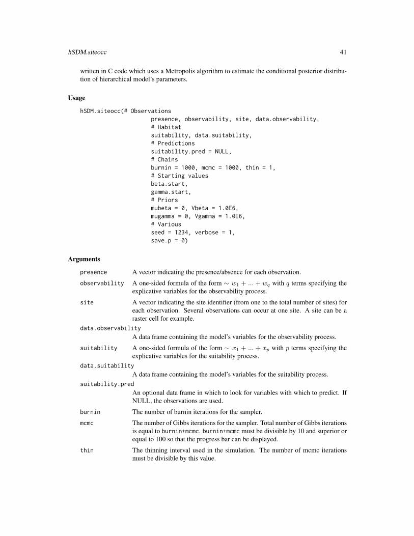
written in C code which uses a Metropolis algorithm to estimate the conditional posterior distribu-tion of hierarchical model’s parameters.
Usage
hSDM.siteocc(# Observationspresence, observability, site, data.observability,# Habitatsuitability, data.suitability,# Predictionssuitability.pred = NULL,# Chainsburnin = 1000, mcmc = 1000, thin = 1,# Starting valuesbeta.start,gamma.start,# Priorsmubeta = 0, Vbeta = 1.0E6,mugamma = 0, Vgamma = 1.0E6,# Variousseed = 1234, verbose = 1,save.p = 0)
Arguments
presence A vector indicating the presence/absence for each observation.
observability A one-sided formula of the form ∼ w1 + ... + wq with q terms specifying theexplicative variables for the observability process.
site A vector indicating the site identifier (from one to the total number of sites) foreach observation. Several observations can occur at one site. A site can be araster cell for example.
data.observability
A data frame containing the model’s variables for the observability process.
suitability A one-sided formula of the form ∼ x1 + ... + xp with p terms specifying theexplicative variables for the suitability process.
data.suitability
A data frame containing the model’s variables for the suitability process.suitability.pred
An optional data frame in which to look for variables with which to predict. IfNULL, the observations are used.
burnin The number of burnin iterations for the sampler.
mcmc The number of Gibbs iterations for the sampler. Total number of Gibbs iterationsis equal to burnin+mcmc. burnin+mcmc must be divisible by 10 and superior orequal to 100 so that the progress bar can be displayed.
thin The thinning interval used in the simulation. The number of mcmc iterationsmust be divisible by this value.

42 hSDM.siteocc
beta.start Starting values for β parameters of the suitability process. This can either be ascalar or a p-length vector.
gamma.start Starting values for β parameters of the observability process. This can either bea scalar or a q-length vector.
mubeta Means of the priors for the β parameters of the suitability process. mubeta mustbe either a scalar or a p-length vector. If mubeta takes a scalar value, then thatvalue will serve as the prior mean for all of the betas. The default value is set to0 for an uninformative prior.
Vbeta Variances of the Normal priors for the β parameters of the suitability process.Vbeta must be either a scalar or a p-length vector. If Vbeta takes a scalar value,then that value will serve as the prior variance for all of the betas. The defaultvariance is large and set to 1.0E6 for an uninformative flat prior.
mugamma Means of the Normal priors for the γ parameters of the observability process.mugamma must be either a scalar or a p-length vector. If mugamma takes a scalarvalue, then that value will serve as the prior mean for all of the gammas. Thedefault value is set to 0 for an uninformative prior.
Vgamma Variances of the Normal priors for the γ parameters of the observability process.Vgamma must be either a scalar or a p-length vector. If Vgamma takes a scalarvalue, then that value will serve as the prior variance for all of the gammas. Thedefault variance is large and set to 1.0E6 for an uninformative flat prior.
seed The seed for the random number generator. Default set to 1234.
verbose A switch (0,1) which determines whether or not the progress of the sampler isprinted to the screen. Default is 1: a progress bar is printed, indicating the step(in %) reached by the Gibbs sampler.
save.p A switch (0,1) which determines whether or not the sampled values for predic-tions are saved. Default is 0: the posterior mean is computed and returned inthe lambda.pred vector. Be careful, setting save.p to 1 might require a largeamount of memory.
Details
The model integrates two processes, an ecological process associated to the presence or absence ofthe species due to habitat suitability and an observation process that takes into account the fact thatthe probability of detection of the species is inferior to one.
Ecological process:zi ∼ Bernoulli(θi)
logit(θi) = Xiβ
Observation process:yit ∼ Bernoulli(zi ∗ δit)
logit(δit) =Witγ
hSDM.siteocc 43
Value
mcmc An mcmc object that contains the posterior sample. This object can be summa-rized by functions provided by the coda package. The posterior sample of thedeviance D, with D = −2 log(
∏it P (yit, Ni|...)), is also provided.
theta.pred If save.p is set to 0 (default), theta.pred is the predictive posterior mean of theprobability associated to the suitability process for each prediction. If save.p isset to 1, theta.pred is an mcmc object with sampled values of the probabilityassociated to the suitability process for each prediction.
theta.latent Predictive posterior mean of the probability associated to the suitability processfor each site.
delta.latent Predictive posterior mean of the probability associated to the observability pro-cess for each observation.
Author(s)
Ghislain Vieilledent <[email protected]>
References
MacKenzie, D. I.; Nichols, J. D.; Lachman, G. B.; Droege, S.; Andrew Royle, J. and Langtimm, C.A. (2002) Estimating site occupancy rates when detection probabilities are less than one. Ecology,83, 2248-2255.
See Also
plot.mcmc, summary.mcmc
Examples
## Not run:
#==============================================# hSDM.siteocc()# Example with simulated data#==============================================
#=================#== Load librarieslibrary(hSDM)
#==================#== Data simulation
#= Number of observation sitesnsite <- 200
#= Set seed for repeatabilityseed <- 4321

44 hSDM.siteocc
#= Ecological process (suitability)set.seed(seed)x1 <- rnorm(nsite,0,1)set.seed(2*seed)x2 <- rnorm(nsite,0,1)X <- cbind(rep(1,nsite),x1,x2)beta.target <- c(-1,1,-1) # Target parameterslogit.theta <- X %*% beta.targettheta <- inv.logit(logit.theta)set.seed(seed)Z <- rbinom(nsite,1,theta)
#= Number of visits associated to each observation pointset.seed(seed)visits <- rpois(nsite,3)visits[visits==0] <- 1# Vector of observation pointssites <- vector()for (i in 1:nsite) {
sites <- c(sites,rep(i,visits[i]))}
#= Observation process (detectability)nobs <- sum(visits)set.seed(seed)w1 <- rnorm(nobs,0,1)set.seed(2*seed)w2 <- rnorm(nobs,0,1)W <- cbind(rep(1,nobs),w1,w2)gamma.target <- c(-1,1,-1) # Target parameterslogit.delta <- W %*% gamma.targetdelta <- inv.logit(logit.delta)set.seed(seed)Y <- rbinom(nobs,1,delta*Z[sites])
#= Data-setsdata.obs <- data.frame(Y,w1,w2,site=sites)data.suit <- data.frame(x1,x2)
#================================#== Parameter inference with hSDM#==================================
Start <- Sys.time() # Start the clockmod.hSDM.siteocc <- hSDM.siteocc(# Observations
presence=data.obs$Y,observability=~w1+w2,site=data.obs$site,data.observability=data.obs,# Habitatsuitability=~x1+x2,data.suitability=data.suit,# Predictions

hSDM.siteocc.iCAR 45
suitability.pred=NULL,# Chainsburnin=2000, mcmc=2000, thin=2,# Starting valuesbeta.start=0,gamma.start=0,# Priorsmubeta=0, Vbeta=1.0E6,mugamma=0, Vgamma=1.0E6,# Variousseed=1234, verbose=1, save.p=0)
Time.hSDM <- difftime(Sys.time(),Start,units="sec") # Time difference
#= Computation timeTime.hSDM
#==========#== Outputs
#= Parameter estimatessummary(mod.hSDM.siteocc$mcmc)pdf(file="Posteriors_hSDM.siteocc.pdf")plot(mod.hSDM.siteocc$mcmc)dev.off()
#= Predictionssummary(mod.hSDM.siteocc$theta.latent)summary(mod.hSDM.siteocc$delta.latent)summary(mod.hSDM.siteocc$theta.pred)pdf(file="Pred-Init.pdf")plot(theta,mod.hSDM.siteocc$theta.pred)abline(a=0,b=1,col="red")dev.off()
## End(Not run)
hSDM.siteocc.iCAR Site-occupancy model with CAR process
Description
The hSDM.siteocc.iCAR function can be used to model species distribution including differentprocesses in a hierarchical Bayesian framework: a Bernoulli suitability process (refering to envi-ronmental suitability) which takes into account the spatial dependence of the observations, and aBernoulli observability process (refering to various ecological and methodological issues explain-ing the species detection). The hSDM.siteocc.iCAR function calls a Gibbs sampler written in Ccode which uses an adaptive Metropolis algorithm to estimate the conditional posterior distributionof hierarchical model’s parameters.
46 hSDM.siteocc.iCAR
Usage
hSDM.siteocc.iCAR(# Observationspresence, observability, site, data.observability,# Habitatsuitability, data.suitability,# Spatial structurespatial.entity,n.neighbors, neighbors,# Predictionssuitability.pred = NULL, spatial.entity.pred = NULL,# Chainsburnin = 1000, mcmc = 1000, thin = 1,# Starting valuesbeta.start,gamma.start,Vrho.start,# Priorsmubeta = 0, Vbeta = 1.0E6,mugamma = 0, Vgamma = 1.0E6,priorVrho = "1/Gamma",shape = 0.5, rate = 0.0005,Vrho.max = 1000,# Variousseed = 1234, verbose = 1,save.rho = 0, save.p = 0)
Arguments
presence A vector indicating the presence/absence for each observation.observability A one-sided formula of the form ∼ w1 + ... + wq with q terms specifying the
explicative variables for the observability process.site A vector indicating the site identifier (from one to the total number of sites) for
each observation. Several observations can occur at one site. A site can be araster cell for example.
data.observability
A data frame containing the model’s variables for the observability process.suitability A one-sided formula of the form ∼ x1 + ... + xp with p terms specifying the
explicative variables for the suitability process.data.suitability
A data frame containing the model’s variables for the suitability process.spatial.entity A vector (of length ’nsite’) indicating the spatial entity identifier for each site.
Values must be between 1 and the total number of spatial entities. Several sitescan be found in one spatial entity. A spatial entity can be a raster cell for exam-ple.
n.neighbors A vector of integers that indicates the number of neighbors (adjacent entities) ofeach spatial entity. length(n.neighbors) indicates the total number of spatialentities.

hSDM.siteocc.iCAR 47
neighbors A vector of integers indicating the neighbors (adjacent entities) of each spatialentity. Must be of the form c(neighbors of entity 1, neighbors of entity 2, ... ,neighbors of the last entity). Length of the neighbors vector should be equal tosum(n.neighbors).
suitability.pred
An optional data frame in which to look for variables with which to predict. IfNULL, the observations are used.
spatial.entity.pred
An optional vector indicating the spatial entity identifier (from one to the totalnumber of entities) for predictions. If NULL, the vector spatial.entity forobservations is used.
burnin The number of burnin iterations for the sampler.
mcmc The number of Gibbs iterations for the sampler. Total number of Gibbs iterationsis equal to burnin+mcmc. burnin+mcmc must be divisible by 10 and superior orequal to 100 so that the progress bar can be displayed.
thin The thinning interval used in the simulation. The number of mcmc iterationsmust be divisible by this value.
beta.start Starting values for β parameters of the suitability process. This can either be ascalar or a p-length vector.
gamma.start Starting values for β parameters of the observability process. This can either bea scalar or a q-length vector.
Vrho.start Positive scalar indicating the starting value for the variance of the spatial randomeffects.
mubeta Means of the priors for the β parameters of the suitability process. mubeta mustbe either a scalar or a p-length vector. If mubeta takes a scalar value, then thatvalue will serve as the prior mean for all of the betas. The default value is set to0 for an uninformative prior.
Vbeta Variances of the Normal priors for the β parameters of the suitability process.Vbeta must be either a scalar or a p-length vector. If Vbeta takes a scalar value,then that value will serve as the prior variance for all of the betas. The defaultvariance is large and set to 1.0E6 for an uninformative flat prior.
mugamma Means of the Normal priors for the γ parameters of the observability process.mugamma must be either a scalar or a p-length vector. If mugamma takes a scalarvalue, then that value will serve as the prior mean for all of the gammas. Thedefault value is set to 0 for an uninformative prior.
Vgamma Variances of the Normal priors for the γ parameters of the observability process.Vgamma must be either a scalar or a p-length vector. If Vgamma takes a scalarvalue, then that value will serve as the prior variance for all of the gammas. Thedefault variance is large and set to 1.0E6 for an uninformative flat prior.
priorVrho Type of prior for the variance of the spatial random effects. Can be set to a fixedpositive scalar, or to an inverse-gamma distribution ("1/Gamma") with param-eters shape and rate, or to a uniform distribution ("Uniform") on the interval[0,Vrho.max]. Default set to "1/Gamma".
shape The shape parameter for the Gamma prior on the precision of the spatial randomeffects. Default value is shape=0.05 for uninformative prior.

48 hSDM.siteocc.iCAR
rate The rate (1/scale) parameter for the Gamma prior on the precision of the spatialrandom effects. Default value is rate=0.0005 for uninformative prior.
Vrho.max Upper bound for the uniform prior of the spatial random effect variance. Defaultset to 1000.
seed The seed for the random number generator. Default set to 1234.
verbose A switch (0,1) which determines whether or not the progress of the sampler isprinted to the screen. Default is 1: a progress bar is printed, indicating the step(in %) reached by the Gibbs sampler.
save.rho A switch (0,1) which determines whether or not the sampled values for rhosare saved. Default is 0: the posterior mean is computed and returned in therho.pred vector. Be careful, setting save.rho to 1 might require a large amountof memory.
save.p A switch (0,1) which determines whether or not the sampled values for predic-tions are saved. Default is 0: the posterior mean is computed and returned inthe theta.pred vector. Be careful, setting save.p to 1 might require a largeamount of memory.
Details
The model integrates two processes, an ecological process associated to the presence or absenceof the species due to habitat suitability and an observation process that takes into account the factthat the probability of detection of the species is inferior to one. The ecological process includesan intrinsic conditional autoregressive model (iCAR) model for spatial autocorrelation betweenobservations, assuming that the probability of presence of the species at one site depends on theprobability of presence of the species on neighboring sites.
Ecological process:zi ∼ Bernoulli(θi)
logit(θi) = Xiβ + ρj(i)
ρj : spatial random effect
j(i): index of the spatial entity for observation i.
Spatial autocorrelation:
An intrinsic conditional autoregressive model (iCAR) is assumed:
ρj ∼ N ormal(µj , Vρ/nj)
µj : mean of ρj′ in the neighborhood of j.
Vρ: variance of the spatial random effects.
nj : number of neighbors for spatial entity j.
Observation process:yit ∼ Bernoulli(zi ∗ δit)
logit(δit) =Witγ
hSDM.siteocc.iCAR 49
Value
mcmc An mcmc object that contains the posterior sample. This object can be summa-rized by functions provided by the coda package. The posterior sample of thedeviance D, with D = −2 log(
∏i P (yi, zi|...)), is also provided.
rho.pred If save.rho is set to 0 (default), rho.pred is the predictive posterior mean ofthe spatial random effect associated to each spatial entity. If save.rho is setto 1, rho.pred is an mcmc object with sampled values for each spatial randomeffect associated to each spatial entity.
theta.pred If save.p is set to 0 (default), theta.pred is the predictive posterior mean of theprobability associated to the suitability process for each prediction. If save.p isset to 1, theta.pred is an mcmc object with sampled values of the probabilityassociated to the suitability process for each prediction.
theta.latent Predictive posterior mean of the probability associated to the suitability processfor each site.
delta.latent Predictive posterior mean of the probability associated to the observability pro-cess for each observation.
Author(s)
Ghislain Vieilledent <[email protected]>
References
Diez, J. M. & Pulliam, H. R. (2007) Hierarchical analysis of species distributions and abundanceacross environmental gradients Ecology, 88, 3144-3152.
Gelfand, A. E.; Schmidt, A. M.; Wu, S.; Silander, J. A.; Latimer, A. and Rebelo, A. G. (2005)Modelling species diversity through species level hierarchical modelling. Applied Statistics, 54,1-20.
Latimer, A. M.; Wu, S. S.; Gelfand, A. E. and Silander, J. A. (2006) Building statistical models toanalyze species distributions. Ecological Applications, 16, 33-50.
Lichstein, J. W.; Simons, T. R.; Shriner, S. A. & Franzreb, K. E. (2002) Spatial autocorrelation andautoregressive models in ecology Ecological Monographs, 72, 445-463.
MacKenzie, D. I.; Nichols, J. D.; Lachman, G. B.; Droege, S.; Andrew Royle, J. and Langtimm, C.A. (2002) Estimating site occupancy rates when detection probabilities are less than one. Ecology,83, 2248-2255.
See Also
plot.mcmc, summary.mcmc
Examples
## Not run:
#==============================================# hSDM.siteocc.iCAR()

50 hSDM.siteocc.iCAR
# Example with simulated data#==============================================
#=================#== Load librarieslibrary(hSDM)library(raster)library(sp)
#===================================#== Multivariate normal distributionrmvn <- function(n, mu = 0, V = matrix(1), seed=1234) {
p <- length(mu)if (any(is.na(match(dim(V), p)))) {
stop("Dimension problem!")}D <- chol(V)set.seed(seed)t(matrix(rnorm(n*p),ncol=p)%*%D+rep(mu,rep(n,p)))
}
#==================#== Data simulation
#= Set seed for repeatabilityseed <- 1234
#= LandscapexLand <- 30yLand <- 30Landscape <- raster(ncol=xLand,nrow=yLand,crs='+proj=utm +zone=1')Landscape[] <- 0extent(Landscape) <- c(0,xLand,0,yLand)coords <- coordinates(Landscape)ncells <- ncell(Landscape)
#= Neighborsneighbors.mat <- adjacent(Landscape, cells=c(1:ncells), directions=8, pairs=TRUE, sorted=TRUE)n.neighbors <- as.data.frame(table(as.factor(neighbors.mat[,1])))[,2]adj <- neighbors.mat[,2]
#= Generate symmetric adjacency matrix, AA <- matrix(0,ncells,ncells)index.start <- 1for (i in 1:ncells) {
index.end <- index.start+n.neighbors[i]-1A[i,adj[c(index.start:index.end)]] <- 1index.start <- index.end+1
}
#= Spatial effectsVrho.target <- 5d <- 1 # Spatial dependence parameter = 1 for intrinsic CAR
hSDM.siteocc.iCAR 51
Q <- diag(n.neighbors)-d*A + diag(.0001,ncells) # Add small constant to make Q non-singularcovrho <- Vrho.target*solve(Q) # Covariance of rhosset.seed(seed)rho <- c(rmvn(1,mu=rep(0,ncells),V=covrho,seed=seed)) # Spatial Random Effectsrho <- rho-mean(rho) # Centering rhos on zero
#= Raster and plot spatial effectsr.rho <- rasterFromXYZ(cbind(coords,rho))plot(r.rho)
#= Sample the observation sites in the landscapensite <- 250set.seed(seed)x.coord <- runif(nsite,0,xLand)set.seed(2*seed)y.coord <- runif(nsite,0,yLand)sites.sp <- SpatialPoints(coords=cbind(x.coord,y.coord))cells <- extract(Landscape,sites.sp,cell=TRUE)[,1]
#= Ecological process (suitability)set.seed(seed)x1 <- rnorm(nsite,0,1)set.seed(2*seed)x2 <- rnorm(nsite,0,1)X <- cbind(rep(1,nsite),x1,x2)beta.target <- c(-1,1,-1)logit.theta <- X %*% beta.target + rho[cells]theta <- inv.logit(logit.theta)set.seed(seed)Z <- rbinom(nsite,1,theta)
#= Relative importance of spatial random effectsRImp <- mean(abs(rho[cells])/abs(X %*% beta.target))RImp
#= Number of visits associated to each observation pointset.seed(seed)visits <- rpois(nsite,3)visits[visits==0] <- 1# Vector of observation pointssites <- vector()for (i in 1:nsite) {
sites <- c(sites,rep(i,visits[i]))}
#= Observation process (detectability)nobs <- sum(visits)set.seed(seed)w1 <- rnorm(nobs,0,1)set.seed(2*seed)w2 <- rnorm(nobs,0,1)W <- cbind(rep(1,nobs),w1,w2)gamma.target <- c(-1,1,-1)
52 hSDM.siteocc.iCAR
logit.delta <- W %*% gamma.targetdelta <- inv.logit(logit.delta)set.seed(seed)Y <- rbinom(nobs,1,delta*Z[sites])
#= Data-setsdata.obs <- data.frame(Y,w1,w2,site=sites)data.suit <- data.frame(x1,x2,cell=cells)
#================================#== Parameter inference with hSDM
Start <- Sys.time() # Start the clockmod.hSDM.siteocc.iCAR <- hSDM.siteocc.iCAR(# Observations
presence=data.obs$Y,observability=~w1+w2,site=data.obs$site,data.observability=data.obs,# Habitat
suitability=~x1+x2, data.suitability=data.suit,# Spatial structurespatial.entity=data.suit$cell,n.neighbors=n.neighbors, neighbors=adj,# Predictionssuitability.pred=NULL,spatial.entity.pred=NULL,# Chainsburnin=10000, mcmc=5000, thin=5,# Starting valuesbeta.start=0,gamma.start=0,Vrho.start=1,# Priorsmubeta=0, Vbeta=1.0E6,mugamma=0, Vgamma=1.0E6,priorVrho="Uniform",Vrho.max=10,# Variousseed=1234, verbose=1,save.rho=1, save.p=0)
Time.hSDM <- difftime(Sys.time(),Start,units="sec") # Time difference
#= Computation timeTime.hSDM
#==========#== Outputs
#= Parameter estimatessummary(mod.hSDM.siteocc.iCAR$mcmc)pdf("Posteriors_hSDM.siteocc.iCAR.pdf")plot(mod.hSDM.siteocc.iCAR$mcmc)dev.off()
hSDM.ZIB 53
#= Predictionssummary(mod.hSDM.siteocc.iCAR$theta.latent)summary(mod.hSDM.siteocc.iCAR$delta.latent)summary(mod.hSDM.siteocc.iCAR$theta.pred)pdf(file="Pred-Init.pdf")plot(theta,mod.hSDM.siteocc.iCAR$theta.pred)abline(a=0,b=1,col="red")dev.off()
#= Summary plots for spatial random effects
# rho.predrho.pred <- apply(mod.hSDM.siteocc.iCAR$rho.pred,2,mean)r.rho.pred <- rasterFromXYZ(cbind(coords,rho.pred))
# plotpdf(file="Summary_hSDM.siteocc.iCAR.pdf")par(mfrow=c(2,2))# rho targetplot(r.rho, main="rho target")plot(sites.sp,add=TRUE)# rho estimatedplot(r.rho.pred, main="rho estimated")# correlation and "shrinkage"Levels.cells <- sort(unique(cells))plot(rho[-Levels.cells],rho.pred[-Levels.cells],
xlim=range(rho),ylim=range(rho),xlab="rho target",ylab="rho estimated")
points(rho[Levels.cells],rho.pred[Levels.cells],pch=16,col="blue")legend(x=-3,y=4,legend="Visited cells",col="blue",pch=16,bty="n")abline(a=0,b=1,col="red")dev.off()
## End(Not run)
hSDM.ZIB ZIB (Zero-Inflated Binomial) model
Description
The hSDM.ZIB function can be used to model species distribution including different processes in ahierarchical Bayesian framework: a Bernoulli suitability process (refering to environmental suit-ability) and a Binomial observability process (refering to various ecological and methodologicalissues explaining the species detection). The hSDM.ZIB function calls a Gibbs sampler written in Ccode which uses a Metropolis algorithm to estimate the conditional posterior distribution of hierar-chical model’s parameters.
54 hSDM.ZIB
Usage
hSDM.ZIB(presences, trials, suitability,observability, data, suitability.pred=NULL, burnin = 5000, mcmc = 10000,thin = 10, beta.start, gamma.start, mubeta = 0, Vbeta = 1e+06, mugamma =0, Vgamma = 1e+06, seed = 1234, verbose = 1, save.p = 0)
Arguments
presences A vector indicating the number of successes (or presences) for each observation.
trials A vector indicating the number of trials for each observation. ti should be supe-rior to zero and superior or equal to yi, the number of successes for observationi.
suitability A one-sided formula of the form ∼ x1 + ... + xp with p terms specifying theexplicative variables for the suitability process.
observability A one-sided formula of the form ∼ w1 + ... + wq with q terms specifying theexplicative variables for the observability process.
data A data frame containing the model’s variables.
suitability.pred
An optional data frame in which to look for variables with which to predict. IfNULL, the observations are used.
burnin The number of burnin iterations for the sampler.
mcmc The number of Gibbs iterations for the sampler. Total number of Gibbs iterationsis equal to burnin+mcmc. burnin+mcmc must be divisible by 10 and superior orequal to 100 so that the progress bar can be displayed.
thin The thinning interval used in the simulation. The number of mcmc iterationsmust be divisible by this value.
beta.start Starting values for β parameters of the suitability process. This can either be ascalar or a p-length vector.
gamma.start Starting values for β parameters of the observability process. This can either bea scalar or a q-length vector.
mubeta Means of the priors for the β parameters of the suitability process. mubeta mustbe either a scalar or a p-length vector. If mubeta takes a scalar value, then thatvalue will serve as the prior mean for all of the betas. The default value is set to0 for an uninformative prior.
Vbeta Variances of the Normal priors for the β parameters of the suitability process.Vbeta must be either a scalar or a p-length vector. If Vbeta takes a scalar value,then that value will serve as the prior variance for all of the betas. The defaultvariance is large and set to 1.0E6 for an uninformative flat prior.
mugamma Means of the Normal priors for the γ parameters of the observability process.mugamma must be either a scalar or a p-length vector. If mugamma takes a scalarvalue, then that value will serve as the prior mean for all of the gammas. Thedefault value is set to 0 for an uninformative prior.

hSDM.ZIB 55
Vgamma Variances of the Normal priors for the γ parameters of the observability process.Vgamma must be either a scalar or a p-length vector. If Vgamma takes a scalarvalue, then that value will serve as the prior variance for all of the gammas. Thedefault variance is large and set to 1.0E6 for an uninformative flat prior.
seed The seed for the random number generator. Default set to 1234.
verbose A switch (0,1) which determines whether or not the progress of the sampler isprinted to the screen. Default is 1: a progress bar is printed, indicating the step(in %) reached by the Gibbs sampler.
save.p A switch (0,1) which determines whether or not the sampled values for predic-tions are saved. Default is 0: the posterior mean is computed and returned inthe prob.p.pred vector. Be careful, setting save.p to 1 might require a largeamount of memory.
Details
The model integrates two processes, an ecological process associated to the presence or absence ofthe species due to habitat suitability and an observation process that takes into account the fact thatthe probability of detection of the species is inferior to one.
Ecological process:zi ∼ Bernoulli(θi)
logit(θi) = Xiβ
Observation process:yi ∼ Binomial(zi ∗ δi, ti)
logit(δi) =Wiγ
Value
mcmc An mcmc object that contains the posterior sample. This object can be summa-rized by functions provided by the coda package. The posterior sample of thedeviance D, with D = −2 log(
∏i P (yi, zi|...)), is also provided.
prob.p.pred If save.p is set to 0 (default), prob.p.pred is the predictive posterior meanof the probability associated to the suitability process for each prediction. Ifsave.p is set to 1, prob.p.pred is an mcmc object with sampled values of theprobability associated to the suitability process for each prediction.
prob.p.latent Predictive posterior mean of the probability associated to the suitability processfor each observation.
prob.q.latent Predictive posterior mean of the probability associated to the observability pro-cess for each observation.
Author(s)
Ghislain Vieilledent <[email protected]>
56 hSDM.ZIB
References
Gelfand, A. E.; Schmidt, A. M.; Wu, S.; Silander, J. A.; Latimer, A. and Rebelo, A. G. (2005)Modelling species diversity through species level hierarchical modelling. Applied Statistics, 54,1-20.
Latimer, A. M.; Wu, S. S.; Gelfand, A. E. and Silander, J. A. (2006) Building statistical models toanalyze species distributions. Ecological Applications, 16, 33-50.
MacKenzie, D. I.; Nichols, J. D.; Lachman, G. B.; Droege, S.; Andrew Royle, J. and Langtimm, C.A. (2002) Estimating site occupancy rates when detection probabilities are less than one. Ecology,83, 2248-2255.
See Also
plot.mcmc, summary.mcmc
Examples
## Not run:
#==============================================# hSDM.ZIB()# Example with simulated data#==============================================
#============#== Preambulelibrary(hSDM)
#==================#== Data simulation
# Set seed for repeatabilityseed <- 1234
# Number of observationsnobs <- 1000
# Target parametersbeta.target <- matrix(c(0.2,0.5,0.5),ncol=1)gamma.target <- matrix(c(1),ncol=1) #= This means that theta.2~0.75: 75% of chance to detect the species## Uncomment if you want covariates on the observability process## gamma.target <- matrix(c(0.2,0.5,0.5),ncol=1)
# Covariates for "suitability" processset.seed(seed)X1 <- rnorm(n=nobs,0,1)set.seed(2*seed)X2 <- rnorm(n=nobs,0,1)X <- cbind(rep(1,nobs),X1,X2)
# Covariates for "observability" process

hSDM.ZIB 57
W <- cbind(rep(1,nobs))## Uncomment if you want covariates on the observability process## set.seed(3*seed)## W1 <- rnorm(n=nobs,0,1)## set.seed(4*seed)## W2 <- rnorm(n=nobs,0,1)## W <- cbind(rep(1,nobs),W1,W2)
#== Simulating latent variables
# Suitabilitylogit.theta.1 <- X %*% beta.targettheta.1 <- inv.logit(logit.theta.1)set.seed(seed)y.1 <- rbinom(nobs,1,theta.1)
# Observabilityset.seed(seed)trials <- rpois(nobs,5) # Number of trial associated to each observationtrials[trials==0] <- 1logit.theta.2 <- W %*% gamma.targettheta.2 <- inv.logit(logit.theta.2)set.seed(seed)y.2 <- rbinom(nobs,trials,theta.2)
#== Simulating response variableY <- y.2*y.1
#== Data-setData <- data.frame(Y,trials,X1,X2)## Uncomment if you want covariates on the observability process## Data <- data.frame(Y,trials,X1,X2,W1,W2)
#==================================#== ZIB model
mod.hSDM.ZIB <- hSDM.ZIB(presences=Data$Y,trials=Data$trials,suitability=~X1+X2,observability=~1, #=~1+W1+W2 if covariatesdata=Data,suitability.pred=NULL,burnin=1000, mcmc=1000, thin=5,beta.start=0,gamma.start=0,mubeta=0, Vbeta=1.0E6,mugamma=0, Vgamma=1.0E6,seed=1234, verbose=1,save.p=0)
#==========#== Outputspdf(file="Posteriors_hSDM.ZIB.pdf")

58 hSDM.ZIB.iCAR
plot(mod.hSDM.ZIB$mcmc)dev.off()summary(mod.hSDM.ZIB$prob.p.latent)summary(mod.hSDM.ZIB$prob.q.latent)summary(mod.hSDM.ZIB$prob.p.pred)
## End(Not run)
hSDM.ZIB.iCAR ZIB (Zero-Inflated Binomial) model with CAR process
Description
The hSDM.ZIB.iCAR function can be used to model species distribution including different pro-cesses in a hierarchical Bayesian framework: a Bernoulli suitability process (refering to envi-ronmental suitability) which takes into account the spatial dependence of the observations, and aBinomial observability process (refering to various ecological and methodological issues explain-ing the species detection). The hSDM.ZIB.iCAR function calls a Gibbs sampler written in C codewhich uses an adaptive Metropolis algorithm to estimate the conditional posterior distribution ofhierarchical model’s parameters.
Usage
hSDM.ZIB.iCAR(presences, trials, suitability,observability, spatial.entity, data, n.neighbors, neighbors,suitability.pred=NULL, spatial.entity.pred=NULL, burnin = 5000, mcmc =10000, thin = 10, beta.start, gamma.start, Vrho.start, mubeta = 0, Vbeta= 1e+06, mugamma = 0, Vgamma = 1e+06, priorVrho = "1/Gamma", shape =0.5, rate = 0.0005, Vrho.max=1000, seed = 1234, verbose = 1, save.rho =0, save.p = 0)
Arguments
presences A vector indicating the number of successes (or presences) for each observation.
trials A vector indicating the number of trials for each observation. ti should be supe-rior to zero and superior or equal to yi, the number of successes for observationi.
suitability A one-sided formula of the form ∼ x1 + ... + xp with p terms specifying theexplicative variables for the suitability process.
observability A one-sided formula of the form ∼ w1 + ... + wq with q terms specifying theexplicative variables for the observability process.
spatial.entity A vector indicating the spatial entity identifier (from one to the total numberof entities) for each observation. Several observations can occur in one spatialentity. A spatial entity can be a raster cell for example.
hSDM.ZIB.iCAR 59
data A data frame containing the model’s variables.
n.neighbors A vector of integers that indicates the number of neighbors (adjacent entities) ofeach spatial entity. length(n.neighbors) indicates the total number of spatialentities.
neighbors A vector of integers indicating the neighbors (adjacent entities) of each spatialentity. Must be of the form c(neighbors of entity 1, neighbors of entity 2, ... ,neighbors of the last entity). Length of the neighbors vector should be equal tosum(n.neighbors).
suitability.pred
An optional data frame in which to look for variables with which to predict. IfNULL, the observations are used.
spatial.entity.pred
An optional vector indicating the spatial entity identifier (from one to the totalnumber of entities) for predictions. If NULL, the vector spatial.entity forobservations is used.
burnin The number of burnin iterations for the sampler.
mcmc The number of Gibbs iterations for the sampler. Total number of Gibbs iterationsis equal to burnin+mcmc. burnin+mcmc must be divisible by 10 and superior orequal to 100 so that the progress bar can be displayed.
thin The thinning interval used in the simulation. The number of mcmc iterationsmust be divisible by this value.
beta.start Starting values for β parameters of the suitability process. This can either be ascalar or a p-length vector.
gamma.start Starting values for β parameters of the observability process. This can either bea scalar or a q-length vector.
Vrho.start Positive scalar indicating the starting value for the variance of the spatial randomeffects.
mubeta Means of the priors for the β parameters of the suitability process. mubeta mustbe either a scalar or a p-length vector. If mubeta takes a scalar value, then thatvalue will serve as the prior mean for all of the betas. The default value is set to0 for an uninformative prior.
Vbeta Variances of the Normal priors for the β parameters of the suitability process.Vbeta must be either a scalar or a p-length vector. If Vbeta takes a scalar value,then that value will serve as the prior variance for all of the betas. The defaultvariance is large and set to 1.0E6 for an uninformative flat prior.
mugamma Means of the Normal priors for the γ parameters of the observability process.mugamma must be either a scalar or a p-length vector. If mugamma takes a scalarvalue, then that value will serve as the prior mean for all of the gammas. Thedefault value is set to 0 for an uninformative prior.
Vgamma Variances of the Normal priors for the γ parameters of the observability process.Vgamma must be either a scalar or a p-length vector. If Vgamma takes a scalarvalue, then that value will serve as the prior variance for all of the gammas. Thedefault variance is large and set to 1.0E6 for an uninformative flat prior.
60 hSDM.ZIB.iCAR
priorVrho Type of prior for the variance of the spatial random effects. Can be set to a fixedpositive scalar, or to an inverse-gamma distribution ("1/Gamma") with param-eters shape and rate, or to a uniform distribution ("Uniform") on the interval[0,Vrho.max]. Default set to "1/Gamma".
shape The shape parameter for the Gamma prior on the precision of the spatial randomeffects. Default value is shape=0.05 for uninformative prior.
rate The rate (1/scale) parameter for the Gamma prior on the precision of the spatialrandom effects. Default value is rate=0.0005 for uninformative prior.
Vrho.max Upper bound for the uniform prior of the spatial random effect variance. Defaultset to 1000.
seed The seed for the random number generator. Default set to 1234.
verbose A switch (0,1) which determines whether or not the progress of the sampler isprinted to the screen. Default is 1: a progress bar is printed, indicating the step(in %) reached by the Gibbs sampler.
save.rho A switch (0,1) which determines whether or not the sampled values for rhosare saved. Default is 0: the posterior mean is computed and returned in therho.pred vector. Be careful, setting save.rho to 1 might require a large amountof memory.
save.p A switch (0,1) which determines whether or not the sampled values for predic-tions are saved. Default is 0: the posterior mean is computed and returned inthe prob.p.pred vector. Be careful, setting save.p to 1 might require a largeamount of memory.
Details
The model integrates two processes, an ecological process associated to the presence or absenceof the species due to habitat suitability and an observation process that takes into account the factthat the probability of detection of the species is inferior to one. The ecological process includesan intrinsic conditional autoregressive model (iCAR) model for spatial autocorrelation betweenobservations, assuming that the probability of presence of the species at one site depends on theprobability of presence of the species on neighboring sites.
Ecological process:zi ∼ Bernoulli(θi)
logit(θi) = Xiβ + ρj(i)
ρj : spatial random effect
j(i): index of the spatial entity for observation i.
Spatial autocorrelation:An intrinsic conditional autoregressive model (iCAR) is assumed:
ρj ∼ N ormal(µj , Vρ/nj)
µj : mean of ρj′ in the neighborhood of j.
Vρ: variance of the spatial random effects.
nj : number of neighbors for spatial entity j.

hSDM.ZIB.iCAR 61
Observation process:yi ∼ Binomial(zi ∗ δi, ti)
logit(δi) =Wiγ
Value
mcmc An mcmc object that contains the posterior sample. This object can be summa-rized by functions provided by the coda package. The posterior sample of thedeviance D, with D = −2 log(
∏i P (yi, zi|...)), is also provided.
rho.pred If save.rho is set to 0 (default), rho.pred is the predictive posterior mean ofthe spatial random effect associated to each spatial entity. If save.rho is setto 1, rho.pred is an mcmc object with sampled values for each spatial randomeffect associated to each spatial entity.
prob.p.pred If save.p is set to 0 (default), prob.p.pred is the predictive posterior meanof the probability associated to the suitability process for each prediction. Ifsave.p is set to 1, prob.p.pred is an mcmc object with sampled values of theprobability associated to the suitability process for each prediction.
prob.p.latent Predictive posterior mean of the probability associated to the suitability processfor each observation.
prob.q.latent Predictive posterior mean of the probability associated to the observability pro-cess for each observation.
Author(s)
Ghislain Vieilledent <[email protected]>
References
Gelfand, A. E.; Schmidt, A. M.; Wu, S.; Silander, J. A.; Latimer, A. and Rebelo, A. G. (2005)Modelling species diversity through species level hierarchical modelling. Applied Statistics, 54,1-20.
Latimer, A. M.; Wu, S. S.; Gelfand, A. E. and Silander, J. A. (2006) Building statistical models toanalyze species distributions. Ecological Applications, 16, 33-50.
MacKenzie, D. I.; Nichols, J. D.; Lachman, G. B.; Droege, S.; Andrew Royle, J. and Langtimm, C.A. (2002) Estimating site occupancy rates when detection probabilities are less than one. Ecology,83, 2248-2255.
See Also
plot.mcmc, summary.mcmc
Examples
## Not run:
#==============================================# hSDM.ZIB.iCAR()
62 hSDM.ZIB.iCAR
# Example with simulated data#==============================================
#============#== Preambulelibrary(hSDM)library(raster)library(sp)library(mvtnorm)
#==================#== Data simulation
# Set seed for repeatabilityseed <- 1234
# Target parametersbeta.target <- matrix(c(0.2,0.5,0.5),ncol=1)gamma.target <- matrix(c(1),ncol=1) #= This means that theta.2~0.75: 75% of chance to detect the species## Uncomment if you want covariates on the observability process## gamma.target <- matrix(c(0.2,0.5,0.5),ncol=1)Vrho.target <- 1 # Spatial Variance
# LandscapeLandscape <- raster(ncol=20,nrow=20,crs='+proj=utm +zone=1')ncell <- ncell(Landscape)
# Neighborsneighbors.mat <- adjacent(Landscape, cells=c(1:ncell), directions=8, pairs=TRUE, sorted=TRUE)n.neighbors <- as.data.frame(table(as.factor(neighbors.mat[,1])))[,2]adj <- neighbors.mat[,2]
# Generate symmetric adjacency matrix, AA <- matrix(0,ncell,ncell)index.start <- 1for (i in 1:ncell) {
index.end <- index.start+n.neighbors[i]-1A[i,adj[c(index.start:index.end)]] <- 1index.start <- index.end+1
}
# Spatial effectsd <- 1 # Spatial dependence parameter = 1 for intrinsic CARQ <- diag(n.neighbors)-d*A + diag(.0001,ncell) # Add small constant to make Q non-singularcovrho <- Vrho.target*solve(Q) # Covariance of rhosset.seed(seed)rho <- c(rmvnorm(1,sigma=covrho)) # Spatial Random Effectsrho <- rho-mean(rho) # Centering rhos on zero
# Visited cellsn.visited <- 150 # Compare with 400, 350 and 100 for exampleset.seed(seed)visited.cells <- sort(sample(1:ncell,n.visited,replace=FALSE)) # Draw visited cells at random
hSDM.ZIB.iCAR 63
notvisited.cells <- c(1:ncell)[-visited.cells]
# Number of observationsnobs <- 300
# Cell vectorset.seed(seed)cells <- c(visited.cells,sample(visited.cells,nobs-n.visited,replace=TRUE))coords <- xyFromCell(Landscape,cells) # Get coordinates
# Covariates for "suitability" processset.seed(seed)X1.cell <- rnorm(n=ncell,0,1) # Here, we decided to define one habitat by spatial entity (raster cell)set.seed(2*seed)X2.cell <- rnorm(n=ncell,0,1)X1 <- X1.cell[cells]X2 <- X2.cell[cells]X <- cbind(rep(1,nobs),X1,X2)
# Covariates for "observability" processW <- cbind(rep(1,nobs))## Uncomment if you want covariates on the observability process## set.seed(3*seed)## W1 <- rnorm(n=nobs,0,1)## set.seed(4*seed)## W2 <- rnorm(n=nobs,0,1)## W <- cbind(rep(1,nobs),W1,W2)
#== Simulating latent variables
# Suitabilitylogit.theta.1 <- vector()for (n in 1:nobs) {
logit.theta.1[n] <- X[n,]%*%beta.target+rho[cells[n]]}theta.1 <- inv.logit(logit.theta.1)set.seed(seed)y.1 <- rbinom(nobs,1,theta.1)
# Observabilityset.seed(seed)trials <- rpois(nobs,5) # Number of trial associated to each observationtrials[trials==0] <- 1logit.theta.2 <- W%*%gamma.targettheta.2 <- inv.logit(logit.theta.2)set.seed(seed)y.2 <- rbinom(nobs,trials,theta.2)
#== Simulating response variableY <- y.2*y.1
#== Data-setData <- data.frame(Y,trials,cells,X1,X2)

64 hSDM.ZIB.iCAR
## Uncomment if you want covariates on the observability process## Data <- data.frame(Y,trials,cells,X1,X2,W1,W2)Data <- SpatialPointsDataFrame(coords=coords,data=Data)plot(Data)
#== Data-set for predictions (suitability on each spatial cell)Data.pred <- data.frame(X1=X1.cell,X2=X2.cell,cells=c(1:ncell))
#==================================#== Site-occupancy model
mod.hSDM.ZIB.iCAR <- hSDM.ZIB.iCAR(presences=Data$Y,trials=Data$trials,suitability=~X1+X2,observability=~1,spatial.entity=Data$cells,data=Data,n.neighbors=n.neighbors,neighbors=adj,## suitability.pred=NULL,## spatial.entity.pred=NULL,suitability.pred=Data.pred,spatial.entity.pred=Data.pred$cells,burnin=5000, mcmc=5000, thin=5,beta.start=0,gamma.start=0,Vrho.start=10,priorVrho="1/Gamma",#priorVrho="Uniform",#priorVrho=10,mubeta=0, Vbeta=1.0E6,mugamma=0, Vgamma=1.0E6,shape=0.5, rate=0.0005,#Vrho.max=1000,seed=1234, verbose=1,save.rho=1, save.p=0)
#==========#== Outputs
#= Parameter estimatessummary(mod.hSDM.ZIB.iCAR$mcmc)
#= MCMC and posteriorspdf(file="Posteriors_hSDM.ZIB.iCAR.pdf")plot(mod.hSDM.ZIB.iCAR$mcmc)dev.off()
pdf(file="Posteriors.rho_hSDM.ZIB.iCAR.pdf")plot(mod.hSDM.ZIB.iCAR$rho.pred)dev.off()
#= Summary plots
hSDM.ZIB.iCAR.alteration 65
# rhor.rho <- r.rho.pred <- r.visited <- Landscaper.rho[] <- rhorho.pred <- apply(mod.hSDM.ZIB.iCAR$rho.pred,2,mean)r.rho.pred[] <- rho.predr.visited[] <- 0r.visited[visited.cells] <- 1# prob.pr.prob.p <- Landscaper.prob.p[] <- mod.hSDM.ZIB.iCAR$prob.p.pred
pdf(file="Summary_hSDM.ZIB.iCAR.pdf")par(mfrow=c(3,2))plot(r.rho, main="rho target")plot(r.visited,main="Visited cells and presences")plot(Data[Y>0,],add=TRUE,pch=16,cex=0.5)plot(r.rho.pred, main="rho estimated")plot(rho[visited.cells],rho.pred[visited.cells],
xlab="rho target",ylab="rho estimated")
points(rho[notvisited.cells],rho.pred[notvisited.cells],pch=16,col="blue")legend(x=-4,y=3.5,legend="Unvisited cells",col="blue",pch=16,bty="n")abline(a=0,b=1,col="red")plot(r.prob.p,main="Proba of presence")plot(Data[Y>0,],add=TRUE,pch=16,cex=0.5)dev.off()
## End(Not run)
hSDM.ZIB.iCAR.alteration
ZIB (Zero-Inflated Binomial) model with CAR process taking into ac-count site alteration
Description
The hSDM.ZIB.iCAR.alteration function can be used to model species distribution including dif-ferent processes in a hierarchical Bayesian framework: (i) a Bernoulli suitability process (referingto environmental suitability) which takes into account the spatial dependence of the observations,(ii) an alteration process (refering to anthropogenic disturbances), and (iii) a Binomial observ-ability process (refering to various ecological and methodological issues explaining the speciesdetection). The hSDM.ZIB.iCAR.alteration function calls a Gibbs sampler written in C codewhich uses an adaptive Metropolis algorithm to estimate the conditional posterior distribution ofhierarchical model’s parameters.

66 hSDM.ZIB.iCAR.alteration
Usage
hSDM.ZIB.iCAR.alteration(presences, trials, suitability,observability, spatial.entity, alteration, data, n.neighbors, neighbors,suitability.pred=NULL, spatial.entity.pred=NULL, burnin = 5000, mcmc =10000, thin = 10, beta.start, gamma.start, Vrho.start, mubeta = 0, Vbeta= 1e+06, mugamma = 0, Vgamma = 1e+06, priorVrho = "1/Gamma", shape =0.5, rate = 0.0005, Vrho.max=1000, seed = 1234, verbose = 1, save.rho =0, save.p = 0)
Arguments
presences A vector indicating the number of successes (or presences) for each observation.
trials A vector indicating the number of trials for each observation. ti should be supe-rior to zero and superior or equal to yi, the number of successes for observationi.
suitability A one-sided formula of the form ∼ x1 + ... + xp with p terms specifying theexplicative variables for the suitability process.
observability A one-sided formula of the form ∼ w1 + ... + wq with q terms specifying theexplicative variables for the observability process.
spatial.entity A vector indicating the spatial entity identifier (from one to the total numberof entities) for each observation. Several observations can occur in one spatialentity. A spatial entity can be a raster cell for example.
alteration A vector indicating the proportion of area in the spatial cell which is transformed(by anthropogenic activities for example) for each observation. Must be between0 and 1.
data A data frame containing the model’s variables.
n.neighbors A vector of integers that indicates the number of neighbors (adjacent entities) ofeach spatial entity. length(n.neighbors) indicates the total number of spatialentities.
neighbors A vector of integers indicating the neighbors (adjacent entities) of each spatialentity. Must be of the form c(neighbors of entity 1, neighbors of entity 2, ... ,neighbors of the last entity). Length of the neighbors vector should be equal tosum(n.neighbors).
suitability.pred
An optional data frame in which to look for variables with which to predict. IfNULL, the observations are used.
spatial.entity.pred
An optional vector indicating the spatial entity identifier (from one to the totalnumber of entities) for predictions. If NULL, the vector spatial.entity forobservations is used.
burnin The number of burnin iterations for the sampler.
mcmc The number of Gibbs iterations for the sampler. Total number of Gibbs iterationsis equal to burnin+mcmc. burnin+mcmc must be divisible by 10 and superior orequal to 100 so that the progress bar can be displayed.
hSDM.ZIB.iCAR.alteration 67
thin The thinning interval used in the simulation. The number of mcmc iterationsmust be divisible by this value.
beta.start Starting values for β parameters of the suitability process. This can either be ascalar or a p-length vector.
gamma.start Starting values for β parameters of the observability process. This can either bea scalar or a q-length vector.
Vrho.start Positive scalar indicating the starting value for the variance of the spatial randomeffects.
mubeta Means of the priors for the β parameters of the suitability process. mubeta mustbe either a scalar or a p-length vector. If mubeta takes a scalar value, then thatvalue will serve as the prior mean for all of the betas. The default value is set to0 for an uninformative prior.
Vbeta Variances of the Normal priors for the β parameters of the suitability process.Vbeta must be either a scalar or a p-length vector. If Vbeta takes a scalar value,then that value will serve as the prior variance for all of the betas. The defaultvariance is large and set to 1.0E6 for an uninformative flat prior.
mugamma Means of the Normal priors for the γ parameters of the observability process.mugamma must be either a scalar or a p-length vector. If mugamma takes a scalarvalue, then that value will serve as the prior mean for all of the gammas. Thedefault value is set to 0 for an uninformative prior.
Vgamma Variances of the Normal priors for the γ parameters of the observability process.Vgamma must be either a scalar or a p-length vector. If Vgamma takes a scalarvalue, then that value will serve as the prior variance for all of the gammas. Thedefault variance is large and set to 1.0E6 for an uninformative flat prior.
priorVrho Type of prior for the variance of the spatial random effects. Can be set to a fixedpositive scalar, or to an inverse-gamma distribution ("1/Gamma") with param-eters shape and rate, or to a uniform distribution ("Uniform") on the interval[0,Vrho.max]. Default set to "1/Gamma".
shape The shape parameter for the Gamma prior on the precision of the spatial randomeffects. Default value is shape=0.05 for uninformative prior.
rate The rate (1/scale) parameter for the Gamma prior on the precision of the spatialrandom effects. Default value is rate=0.0005 for uninformative prior.
Vrho.max Upper bound for the uniform prior of the spatial random effect variance. Defaultset to 1000.
seed The seed for the random number generator. Default set to 1234.verbose A switch (0,1) which determines whether or not the progress of the sampler is
printed to the screen. Default is 1: a progress bar is printed, indicating the step(in %) reached by the Gibbs sampler.
save.rho A switch (0,1) which determines whether or not the sampled values for rhosare saved. Default is 0: the posterior mean is computed and returned in therho.pred vector. Be careful, setting save.rho to 1 might require a large amountof memory.
save.p A switch (0,1) which determines whether or not the sampled values for predic-tions are saved. Default is 0: the posterior mean is computed and returned inthe prob.p.pred vector. Be careful, setting save.p to 1 might require a largeamount of memory.

68 hSDM.ZIB.iCAR.alteration
Details
The model integrates two processes, an ecological process associated to the presence or absenceof the species due to habitat suitability and an observation process that takes into account the factthat the probability of detection of the species is inferior to one. The ecological process includesan intrinsic conditional autoregressive model (iCAR) model for spatial autocorrelation betweenobservations, assuming that the probability of presence of the species at one site depends on theprobability of presence of the species on neighboring sites.
Ecological process:zi ∼ Bernoulli(θi)
logit(θi) = Xiβ + ρj(i)
ρj : spatial random effect
j(i): index of the spatial entity for observation i.
Spatial autocorrelation:An intrinsic conditional autoregressive model (iCAR) is assumed:
ρj ∼ N ormal(µj , Vρ/nj)
µj : mean of ρj′ in the neighborhood of j.
Vρ: variance of the spatial random effects.
nj : number of neighbors for spatial entity j.
Observation process:yi ∼ Binomial(zi ∗ δi, ti)
logit(δi) =Wiγ
Value
mcmc An mcmc object that contains the posterior sample. This object can be summa-rized by functions provided by the coda package. The posterior sample of thedeviance D, with D = −2 log(
∏i P (yi, zi|...)), is also provided.
rho.pred If save.rho is set to 0 (default), rho.pred is the predictive posterior mean ofthe spatial random effect associated to each spatial entity. If save.rho is setto 1, rho.pred is an mcmc object with sampled values for each spatial randomeffect associated to each spatial entity.
prob.p.pred If save.p is set to 0 (default), prob.p.pred is the predictive posterior meanof the probability associated to the suitability process for each prediction. Ifsave.p is set to 1, prob.p.pred is an mcmc object with sampled values of theprobability associated to the suitability process for each prediction.
prob.p.latent Predictive posterior mean of the probability associated to the suitability processfor each observation.
prob.q.latent Predictive posterior mean of the probability associated to the observability pro-cess for each observation.
Author(s)
Ghislain Vieilledent <[email protected]>
hSDM.ZIB.iCAR.alteration 69
References
Gelfand, A. E.; Schmidt, A. M.; Wu, S.; Silander, J. A.; Latimer, A. and Rebelo, A. G. (2005)Modelling species diversity through species level hierarchical modelling. Applied Statistics, 54,1-20.
Latimer, A. M.; Wu, S. S.; Gelfand, A. E. and Silander, J. A. (2006) Building statistical models toanalyze species distributions. Ecological Applications, 16, 33-50.
MacKenzie, D. I.; Nichols, J. D.; Lachman, G. B.; Droege, S.; Andrew Royle, J. and Langtimm, C.A. (2002) Estimating site occupancy rates when detection probabilities are less than one. Ecology,83, 2248-2255.
See Also
plot.mcmc, summary.mcmc
Examples
## Not run:
#==============================================# hSDM.ZIB.iCAR.alteration()# Example with simulated data#==============================================
#============#== Preambulelibrary(hSDM)library(raster)library(sp)library(mvtnorm)
#==================#== Data simulation
# Set seed for repeatabilityseed <- 1234
# Target parametersbeta.target <- matrix(c(0.2,0.5,0.5),ncol=1)gamma.target <- matrix(c(1),ncol=1) #= This means that theta.2~0.75: 75% of chance to detect the species## Uncomment if you want covariates on the observability process## gamma.target <- matrix(c(0.2,0.5,0.5),ncol=1)Vrho.target <- 1 # Spatial Variance
# LandscapeLandscape <- raster(ncol=20,nrow=20,crs='+proj=utm +zone=1')ncell <- ncell(Landscape)
# Neighborsneighbors.mat <- adjacent(Landscape, cells=c(1:ncell), directions=8, pairs=TRUE, sorted=TRUE)n.neighbors <- as.data.frame(table(as.factor(neighbors.mat[,1])))[,2]
70 hSDM.ZIB.iCAR.alteration
adj <- neighbors.mat[,2]
# Generate symmetric adjacency matrix, AA <- matrix(0,ncell,ncell)index.start <- 1for (i in 1:ncell) {
index.end <- index.start+n.neighbors[i]-1A[i,adj[c(index.start:index.end)]] <- 1index.start <- index.end+1
}
# Spatial effectsd <- 1 # Spatial dependence parameter = 1 for intrinsic CARQ <- diag(n.neighbors)-d*A + diag(.0001,ncell) # Add small constant to make Q non-singularcovrho <- Vrho.target*solve(Q) # Covariance of rhosset.seed(seed)rho <- c(rmvnorm(1,sigma=covrho)) # Spatial Random Effectsrho <- rho-mean(rho) # Centering rhos on zero
# Visited cellsn.visited <- 150 # Compare with 400, 350 and 100 for exampleset.seed(seed)visited.cells <- sort(sample(1:ncell,n.visited,replace=FALSE)) # Draw visited cells at randomnotvisited.cells <- c(1:ncell)[-visited.cells]
# Number of observationsnobs <- 300
# Cell vectorset.seed(seed)cells <- c(visited.cells,sample(visited.cells,nobs-n.visited,replace=TRUE))coords <- xyFromCell(Landscape,cells) # Get coordinates
# Covariates for "suitability" processset.seed(seed)X1.cell <- rnorm(n=ncell,0,1) # Here, we decided to define one habitat by spatial entity (raster cell)set.seed(2*seed)X2.cell <- rnorm(n=ncell,0,1)X1 <- X1.cell[cells]X2 <- X2.cell[cells]X <- cbind(rep(1,nobs),X1,X2)
# AlterationU <- runif(n=nobs,min=0,max=1)
# Covariates for "observability" processW <- cbind(rep(1,nobs))## Uncomment if you want covariates on the observability process## set.seed(3*seed)## W1 <- rnorm(n=nobs,0,1)## set.seed(4*seed)## W2 <- rnorm(n=nobs,0,1)## W <- cbind(rep(1,nobs),W1,W2)
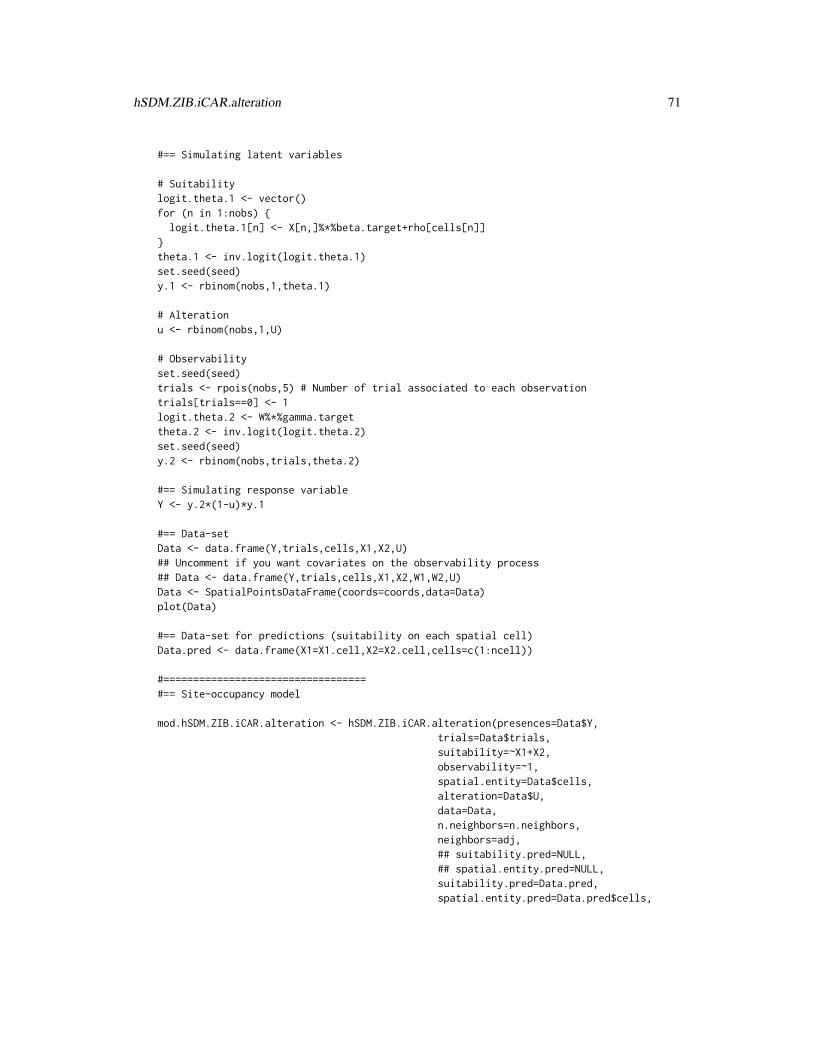
hSDM.ZIB.iCAR.alteration 71
#== Simulating latent variables
# Suitabilitylogit.theta.1 <- vector()for (n in 1:nobs) {
logit.theta.1[n] <- X[n,]%*%beta.target+rho[cells[n]]}theta.1 <- inv.logit(logit.theta.1)set.seed(seed)y.1 <- rbinom(nobs,1,theta.1)
# Alterationu <- rbinom(nobs,1,U)
# Observabilityset.seed(seed)trials <- rpois(nobs,5) # Number of trial associated to each observationtrials[trials==0] <- 1logit.theta.2 <- W%*%gamma.targettheta.2 <- inv.logit(logit.theta.2)set.seed(seed)y.2 <- rbinom(nobs,trials,theta.2)
#== Simulating response variableY <- y.2*(1-u)*y.1
#== Data-setData <- data.frame(Y,trials,cells,X1,X2,U)## Uncomment if you want covariates on the observability process## Data <- data.frame(Y,trials,cells,X1,X2,W1,W2,U)Data <- SpatialPointsDataFrame(coords=coords,data=Data)plot(Data)
#== Data-set for predictions (suitability on each spatial cell)Data.pred <- data.frame(X1=X1.cell,X2=X2.cell,cells=c(1:ncell))
#==================================#== Site-occupancy model
mod.hSDM.ZIB.iCAR.alteration <- hSDM.ZIB.iCAR.alteration(presences=Data$Y,trials=Data$trials,suitability=~X1+X2,observability=~1,spatial.entity=Data$cells,alteration=Data$U,data=Data,n.neighbors=n.neighbors,neighbors=adj,## suitability.pred=NULL,## spatial.entity.pred=NULL,suitability.pred=Data.pred,spatial.entity.pred=Data.pred$cells,

72 hSDM.ZIB.iCAR.alteration
burnin=5000, mcmc=5000, thin=5,beta.start=0,gamma.start=0,Vrho.start=10,priorVrho="1/Gamma",#priorVrho="Uniform",#priorVrho=10,mubeta=0, Vbeta=1.0E6,mugamma=0, Vgamma=1.0E6,shape=0.5, rate=0.0005,#Vrho.max=1000,seed=1234, verbose=1,save.rho=1, save.p=0)
#==========#== Outputs
#= Parameter estimatessummary(mod.hSDM.ZIB.iCAR.alteration$mcmc)
#= MCMC and posteriorspdf(file="Posteriors_hSDM.ZIB.iCAR.alteration.pdf")plot(mod.hSDM.ZIB.iCAR.alteration$mcmc)dev.off()
pdf(file="Posteriors.rho_hSDM.ZIB.iCAR.alteration.pdf")plot(mod.hSDM.ZIB.iCAR.alteration$rho.pred)dev.off()
#= Summary plots
# rhor.rho <- r.rho.pred <- r.visited <- Landscaper.rho[] <- rhorho.pred <- apply(mod.hSDM.ZIB.iCAR.alteration$rho.pred,2,mean)r.rho.pred[] <- rho.predr.visited[] <- 0r.visited[visited.cells] <- 1# prob.pr.prob.p <- Landscaper.prob.p[] <- mod.hSDM.ZIB.iCAR.alteration$prob.p.pred
pdf(file="Summary_hSDM.ZIB.iCAR.alteration.pdf")par(mfrow=c(3,2))plot(r.rho, main="rho target")plot(r.visited,main="Visited cells and presences")plot(Data[Y>0,],add=TRUE,pch=16,cex=0.5)plot(r.rho.pred, main="rho estimated")plot(rho[visited.cells],rho.pred[visited.cells],
xlab="rho target",ylab="rho estimated")
points(rho[notvisited.cells],rho.pred[notvisited.cells],pch=16,col="blue")legend(x=-4,y=3.5,legend="Unvisited cells",col="blue",pch=16,bty="n")

hSDM.ZIP 73
abline(a=0,b=1,col="red")plot(r.prob.p,main="Proba of presence")plot(Data[Y>0,],add=TRUE,pch=16,cex=0.5)dev.off()
## End(Not run)
hSDM.ZIP ZIP (Zero-Inflated Poisson) model
Description
The hSDM.ZIP function can be used to model species distribution including different processes ina hierarchical Bayesian framework: a Bernoulli suitability process (refering to various ecologicalvariables explaining environmental suitability or not) and a Poisson abundance process (referingto various ecological variables explaining the species abundance when the habitat is suitable). ThehSDM.ZIP function calls a Gibbs sampler written in C code which uses a Metropolis algorithm toestimate the conditional posterior distribution of hierarchical model’s parameters.
Usage
hSDM.ZIP(counts, suitability, abundance, data,suitability.pred=NULL, burnin = 5000, mcmc = 10000, thin = 10,beta.start, gamma.start, mubeta = 0, Vbeta = 1e+06, mugamma = 0, Vgamma= 1e+06, seed = 1234, verbose = 1, save.p = 0)
Arguments
counts A vector indicating the count for each observation.
suitability A one-sided formula of the form ∼ x1 + ... + xp with p terms specifying theexplicative variables for the suitability process.
abundance A one-sided formula of the form ∼ w1 + ... + wq with q terms specifying theexplicative variables for the abundance process.
data A data frame containing the model’s variables.suitability.pred
An optional data frame in which to look for variables with which to predict. IfNULL, the observations are used.
burnin The number of burnin iterations for the sampler.
mcmc The number of Gibbs iterations for the sampler. Total number of Gibbs iterationsis equal to burnin+mcmc. burnin+mcmc must be divisible by 10 and superior orequal to 100 so that the progress bar can be displayed.
thin The thinning interval used in the simulation. The number of mcmc iterationsmust be divisible by this value.

74 hSDM.ZIP
beta.start Starting values for β parameters of the suitability process. This can either be ascalar or a p-length vector.
gamma.start Starting values for β parameters of the abundance process. This can either be ascalar or a q-length vector.
mubeta Means of the priors for the β parameters of the suitability process. mubeta mustbe either a scalar or a p-length vector. If mubeta takes a scalar value, then thatvalue will serve as the prior mean for all of the betas. The default value is set to0 for an uninformative prior.
Vbeta Variances of the Normal priors for the β parameters of the suitability process.Vbeta must be either a scalar or a p-length vector. If Vbeta takes a scalar value,then that value will serve as the prior variance for all of the betas. The defaultvariance is large and set to 1.0E6 for an uninformative flat prior.
mugamma Means of the Normal priors for the γ parameters of the abundance process.mugamma must be either a scalar or a p-length vector. If mugamma takes a scalarvalue, then that value will serve as the prior mean for all of the gammas. Thedefault value is set to 0 for an uninformative prior.
Vgamma Variances of the Normal priors for the γ parameters of the abundance process.Vgamma must be either a scalar or a p-length vector. If Vgamma takes a scalarvalue, then that value will serve as the prior variance for all of the gammas. Thedefault variance is large and set to 1.0E6 for an uninformative flat prior.
seed The seed for the random number generator. Default set to 1234.
verbose A switch (0,1) which determines whether or not the progress of the sampler isprinted to the screen. Default is 1: a progress bar is printed, indicating the step(in %) reached by the Gibbs sampler.
save.p A switch (0,1) which determines whether or not the sampled values for predic-tions are saved. Default is 0: the posterior mean is computed and returned inthe prob.p.pred vector. Be careful, setting save.p to 1 might require a largeamount of memory.
Details
The model integrates two processes, an ecological process associated to habitat suitability (habitat issuitable or not for the species) and an abundance process that takes into account ecological variablesexplaining the species abundance when the habitat is suitable.
Suitability process:zi ∼ Bernoulli(θi)
logit(θi) = Xiβ
Abundance process:yi ∼ Poisson(zi ∗ λi)
log(λi) =Wiγ

hSDM.ZIP 75
Value
mcmc An mcmc object that contains the posterior sample. This object can be summa-rized by functions provided by the coda package. The posterior sample of thedeviance D, with D = −2 log(
∏i P (yi, zi|...)), is also provided.
prob.p.pred If save.p is set to 0 (default), prob.p.pred is the predictive posterior meanof the probability associated to the suitability process for each prediction. Ifsave.p is set to 1, prob.p.pred is an mcmc object with sampled values of theprobability associated to the suitability process for each prediction.
prob.p.latent Predictive posterior mean of the probability associated to the suitability processfor each observation.
prob.q.latent Predictive posterior mean of the probability associated to the abundance processfor each observation.
Author(s)
Ghislain Vieilledent <[email protected]>
References
Flores, O.; Rossi, V. and Mortier, F. (2009) Autocorrelation offsets zero-inflation in models oftropical saplings density. Ecological Modelling, 220, 1797-1809.
Gelfand, A. E.; Schmidt, A. M.; Wu, S.; Silander, J. A.; Latimer, A. and Rebelo, A. G. (2005)Modelling species diversity through species level hierarchical modelling. Applied Statistics, 54,1-20.
Latimer, A. M.; Wu, S. S.; Gelfand, A. E. and Silander, J. A. (2006) Building statistical models toanalyze species distributions. Ecological Applications, 16, 33-50.
See Also
plot.mcmc, summary.mcmc
Examples
## Not run:
#==============================================# hSDM.ZIP()# Example with simulated data#==============================================
#============#== Preambulelibrary(hSDM)
#==================#== Data simulation
# Set seed for repeatability

76 hSDM.ZIP
seed <- 1234
# Number of observationsnobs <- 1000
# Target parametersbeta.target <- matrix(c(0.2,0.5,0.5),ncol=1)gamma.target <- matrix(c(1),ncol=1)## Uncomment if you want covariates on the abundance process## gamma.target <- matrix(c(0.2,0.5,0.5),ncol=1)
# Covariates for "suitability" processset.seed(seed)X1 <- rnorm(n=nobs,0,1)set.seed(2*seed)X2 <- rnorm(n=nobs,0,1)X <- cbind(rep(1,nobs),X1,X2)
# Covariates for "abundance" processW <- cbind(rep(1,nobs))## Uncomment if you want covariates on the abundance process## set.seed(3*seed)## W1 <- rnorm(n=nobs,0,1)## set.seed(4*seed)## W2 <- rnorm(n=nobs,0,1)## W <- cbind(rep(1,nobs),W1,W2)
#== Simulating latent variables
# Suitabilitylogit.theta <- X %*% beta.targettheta <- inv.logit(logit.theta)set.seed(seed)y.1 <- rbinom(nobs,1,theta)
# Abundanceset.seed(seed)log.lambda <- W %*% gamma.targetlambda <- exp(log.lambda)set.seed(seed)y.2 <- rpois(nobs,lambda)
#== Simulating response variableY <- y.2*y.1
#== Data-setData <- data.frame(Y,X1,X2)## Uncomment if you want covariates on the abundance process## Data <- data.frame(Y,X1,X2,W1,W2)
#==================================#== ZIP model
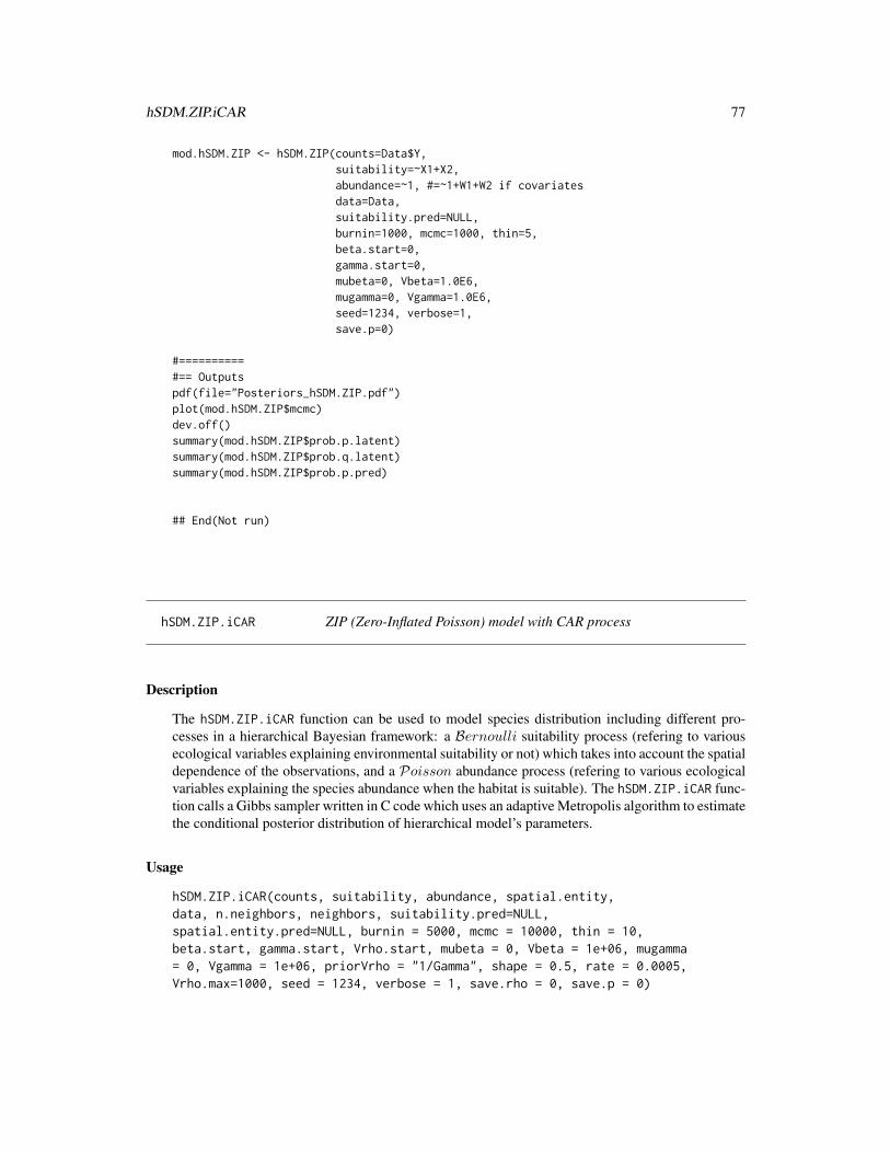
hSDM.ZIP.iCAR 77
mod.hSDM.ZIP <- hSDM.ZIP(counts=Data$Y,suitability=~X1+X2,abundance=~1, #=~1+W1+W2 if covariatesdata=Data,suitability.pred=NULL,burnin=1000, mcmc=1000, thin=5,beta.start=0,gamma.start=0,mubeta=0, Vbeta=1.0E6,mugamma=0, Vgamma=1.0E6,seed=1234, verbose=1,save.p=0)
#==========#== Outputspdf(file="Posteriors_hSDM.ZIP.pdf")plot(mod.hSDM.ZIP$mcmc)dev.off()summary(mod.hSDM.ZIP$prob.p.latent)summary(mod.hSDM.ZIP$prob.q.latent)summary(mod.hSDM.ZIP$prob.p.pred)
## End(Not run)
hSDM.ZIP.iCAR ZIP (Zero-Inflated Poisson) model with CAR process
Description
The hSDM.ZIP.iCAR function can be used to model species distribution including different pro-cesses in a hierarchical Bayesian framework: a Bernoulli suitability process (refering to variousecological variables explaining environmental suitability or not) which takes into account the spatialdependence of the observations, and a Poisson abundance process (refering to various ecologicalvariables explaining the species abundance when the habitat is suitable). The hSDM.ZIP.iCAR func-tion calls a Gibbs sampler written in C code which uses an adaptive Metropolis algorithm to estimatethe conditional posterior distribution of hierarchical model’s parameters.
Usage
hSDM.ZIP.iCAR(counts, suitability, abundance, spatial.entity,data, n.neighbors, neighbors, suitability.pred=NULL,spatial.entity.pred=NULL, burnin = 5000, mcmc = 10000, thin = 10,beta.start, gamma.start, Vrho.start, mubeta = 0, Vbeta = 1e+06, mugamma= 0, Vgamma = 1e+06, priorVrho = "1/Gamma", shape = 0.5, rate = 0.0005,Vrho.max=1000, seed = 1234, verbose = 1, save.rho = 0, save.p = 0)
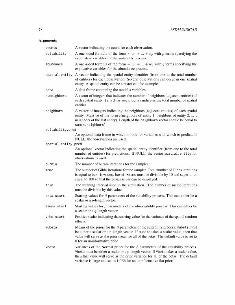
78 hSDM.ZIP.iCAR
Arguments
counts A vector indicating the count for each observation.
suitability A one-sided formula of the form ∼ x1 + ... + xp with p terms specifying theexplicative variables for the suitability process.
abundance A one-sided formula of the form ∼ w1 + ... + wq with q terms specifying theexplicative variables for the abundance process.
spatial.entity A vector indicating the spatial entity identifier (from one to the total numberof entities) for each observation. Several observations can occur in one spatialentity. A spatial entity can be a raster cell for example.
data A data frame containing the model’s variables.
n.neighbors A vector of integers that indicates the number of neighbors (adjacent entities) ofeach spatial entity. length(n.neighbors) indicates the total number of spatialentities.
neighbors A vector of integers indicating the neighbors (adjacent entities) of each spatialentity. Must be of the form c(neighbors of entity 1, neighbors of entity 2, ... ,neighbors of the last entity). Length of the neighbors vector should be equal tosum(n.neighbors).
suitability.pred
An optional data frame in which to look for variables with which to predict. IfNULL, the observations are used.
spatial.entity.pred
An optional vector indicating the spatial entity identifier (from one to the totalnumber of entities) for predictions. If NULL, the vector spatial.entity forobservations is used.
burnin The number of burnin iterations for the sampler.
mcmc The number of Gibbs iterations for the sampler. Total number of Gibbs iterationsis equal to burnin+mcmc. burnin+mcmc must be divisible by 10 and superior orequal to 100 so that the progress bar can be displayed.
thin The thinning interval used in the simulation. The number of mcmc iterationsmust be divisible by this value.
beta.start Starting values for β parameters of the suitability process. This can either be ascalar or a p-length vector.
gamma.start Starting values for β parameters of the observability process. This can either bea scalar or a q-length vector.
Vrho.start Positive scalar indicating the starting value for the variance of the spatial randomeffects.
mubeta Means of the priors for the β parameters of the suitability process. mubeta mustbe either a scalar or a p-length vector. If mubeta takes a scalar value, then thatvalue will serve as the prior mean for all of the betas. The default value is set to0 for an uninformative prior.
Vbeta Variances of the Normal priors for the β parameters of the suitability process.Vbeta must be either a scalar or a p-length vector. If Vbeta takes a scalar value,then that value will serve as the prior variance for all of the betas. The defaultvariance is large and set to 1.0E6 for an uninformative flat prior.

hSDM.ZIP.iCAR 79
mugamma Means of the Normal priors for the γ parameters of the observability process.mugamma must be either a scalar or a p-length vector. If mugamma takes a scalarvalue, then that value will serve as the prior mean for all of the gammas. Thedefault value is set to 0 for an uninformative prior.
Vgamma Variances of the Normal priors for the γ parameters of the observability process.Vgamma must be either a scalar or a p-length vector. If Vgamma takes a scalarvalue, then that value will serve as the prior variance for all of the gammas. Thedefault variance is large and set to 1.0E6 for an uninformative flat prior.
priorVrho Type of prior for the variance of the spatial random effects. Can be set to a fixedpositive scalar, or to an inverse-gamma distribution ("1/Gamma") with param-eters shape and rate, or to a uniform distribution ("Uniform") on the interval[0,Vrho.max]. Default set to "1/Gamma".
shape The shape parameter for the Gamma prior on the precision of the spatial randomeffects. Default value is shape=0.05 for uninformative prior.
rate The rate (1/scale) parameter for the Gamma prior on the precision of the spatialrandom effects. Default value is rate=0.0005 for uninformative prior.
Vrho.max Upper bound for the uniform prior of the spatial random effect variance. Defaultset to 1000.
seed The seed for the random number generator. Default set to 1234.
verbose A switch (0,1) which determines whether or not the progress of the sampler isprinted to the screen. Default is 1: a progress bar is printed, indicating the step(in %) reached by the Gibbs sampler.
save.rho A switch (0,1) which determines whether or not the sampled values for rhosare saved. Default is 0: the posterior mean is computed and returned in therho.pred vector. Be careful, setting save.rho to 1 might require a large amountof memory.
save.p A switch (0,1) which determines whether or not the sampled values for predic-tions are saved. Default is 0: the posterior mean is computed and returned inthe prob.p.pred vector. Be careful, setting save.p to 1 might require a largeamount of memory.
Details
The model integrates two processes, an ecological process associated to habitat suitability (habitat issuitable or not for the species) and an abundance process that takes into account ecological variablesexplaining the species abundance when the habitat is suitable. The suitability process includesan intrinsic conditional autoregressive model (iCAR) model for spatial autocorrelation betweenobservations, assuming that the suitability at one site depends on the suitability on neighboringsites.
Suitability process:zi ∼ Bernoulli(θi)
logit(θi) = Xiβ + ρj(i)
ρj : spatial random effect
j(i): index of the spatial entity for observation i.

80 hSDM.ZIP.iCAR
Spatial autocorrelation:An intrinsic conditional autoregressive model (iCAR) is assumed:
ρj ∼ N ormal(µj , Vρ/nj)
µj : mean of ρj′ in the neighborhood of j.
Vρ: variance of the spatial random effects.
nj : number of neighbors for spatial entity j.
Abundance process:yi ∼ Poisson(zi ∗ λi)
log(λi) =Wiγ
Value
mcmc An mcmc object that contains the posterior sample. This object can be summa-rized by functions provided by the coda package. The posterior sample of thedeviance D, with D = −2 log(
∏i P (yi, zi|...)), is also provided.
rho.pred If save.rho is set to 0 (default), rho.pred is the predictive posterior mean ofthe spatial random effect associated to each spatial entity. If save.rho is setto 1, rho.pred is an mcmc object with sampled values for each spatial randomeffect associated to each spatial entity.
prob.p.pred If save.p is set to 0 (default), prob.p.pred is the predictive posterior meanof the probability associated to the suitability process for each prediction. Ifsave.p is set to 1, prob.p.pred is an mcmc object with sampled values of theprobability associated to the suitability process for each prediction.
prob.p.latent Predictive posterior mean of the probability associated to the suitability processfor each observation.
prob.q.latent Predictive posterior mean of the probability associated to the observability pro-cess for each observation.
Author(s)
Ghislain Vieilledent <[email protected]>
References
Flores, O.; Rossi, V. and Mortier, F. (2009) Autocorrelation offsets zero-inflation in models oftropical saplings density. Ecological Modelling, 220, 1797-1809.
Gelfand, A. E.; Schmidt, A. M.; Wu, S.; Silander, J. A.; Latimer, A. and Rebelo, A. G. (2005)Modelling species diversity through species level hierarchical modelling. Applied Statistics, 54,1-20.
Latimer, A. M.; Wu, S. S.; Gelfand, A. E. and Silander, J. A. (2006) Building statistical models toanalyze species distributions. Ecological Applications, 16, 33-50.
See Also
plot.mcmc, summary.mcmc
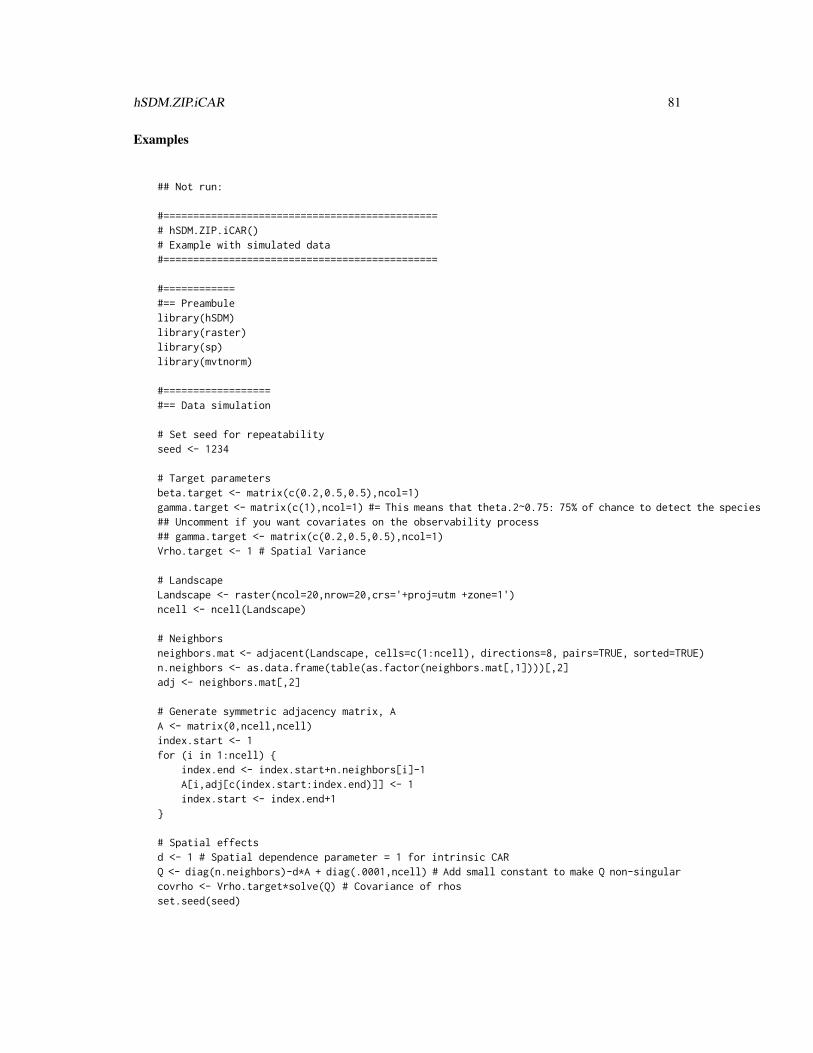
hSDM.ZIP.iCAR 81
Examples
## Not run:
#==============================================# hSDM.ZIP.iCAR()# Example with simulated data#==============================================
#============#== Preambulelibrary(hSDM)library(raster)library(sp)library(mvtnorm)
#==================#== Data simulation
# Set seed for repeatabilityseed <- 1234
# Target parametersbeta.target <- matrix(c(0.2,0.5,0.5),ncol=1)gamma.target <- matrix(c(1),ncol=1) #= This means that theta.2~0.75: 75% of chance to detect the species## Uncomment if you want covariates on the observability process## gamma.target <- matrix(c(0.2,0.5,0.5),ncol=1)Vrho.target <- 1 # Spatial Variance
# LandscapeLandscape <- raster(ncol=20,nrow=20,crs='+proj=utm +zone=1')ncell <- ncell(Landscape)
# Neighborsneighbors.mat <- adjacent(Landscape, cells=c(1:ncell), directions=8, pairs=TRUE, sorted=TRUE)n.neighbors <- as.data.frame(table(as.factor(neighbors.mat[,1])))[,2]adj <- neighbors.mat[,2]
# Generate symmetric adjacency matrix, AA <- matrix(0,ncell,ncell)index.start <- 1for (i in 1:ncell) {
index.end <- index.start+n.neighbors[i]-1A[i,adj[c(index.start:index.end)]] <- 1index.start <- index.end+1
}
# Spatial effectsd <- 1 # Spatial dependence parameter = 1 for intrinsic CARQ <- diag(n.neighbors)-d*A + diag(.0001,ncell) # Add small constant to make Q non-singularcovrho <- Vrho.target*solve(Q) # Covariance of rhosset.seed(seed)

82 hSDM.ZIP.iCAR
rho <- c(rmvnorm(1,sigma=covrho)) # Spatial Random Effectsrho <- rho-mean(rho) # Centering rhos on zero
# Visited cellsn.visited <- 150 # Compare with 400, 350 and 100 for exampleset.seed(seed)visited.cells <- sort(sample(1:ncell,n.visited,replace=FALSE)) # Draw visited cells at randomnotvisited.cells <- c(1:ncell)[-visited.cells]
# Number of observationsnobs <- 300
# Cell vectorset.seed(seed)cells <- c(visited.cells,sample(visited.cells,nobs-n.visited,replace=TRUE))coords <- xyFromCell(Landscape,cells) # Get coordinates
# Covariates for "suitability" processset.seed(seed)X1.cell <- rnorm(n=ncell,0,1) # Here, we decided to define one habitat by spatial entity (raster cell)set.seed(2*seed)X2.cell <- rnorm(n=ncell,0,1)X1 <- X1.cell[cells]X2 <- X2.cell[cells]X <- cbind(rep(1,nobs),X1,X2)
# Covariates for "abundance" processW <- cbind(rep(1,nobs))## Uncomment if you want covariates on the observability process## set.seed(3*seed)## W1 <- rnorm(n=nobs,0,1)## set.seed(4*seed)## W2 <- rnorm(n=nobs,0,1)## W <- cbind(rep(1,nobs),W1,W2)
#== Simulating latent variables
# Suitabilitylogit.theta <- vector()for (n in 1:nobs) {
logit.theta[n] <- X[n,]%*%beta.target+rho[cells[n]]}theta <- inv.logit(logit.theta)set.seed(seed)y.1 <- rbinom(nobs,1,theta)
# Abundanceset.seed(seed)log.lambda <- W %*% gamma.targetlambda <- exp(log.lambda)set.seed(seed)y.2 <- rpois(nobs,lambda)

hSDM.ZIP.iCAR 83
#== Simulating response variableY <- y.2*y.1
#== Data-setData <- data.frame(Y,cells,X1,X2)## Uncomment if you want covariates on the observability process## Data <- data.frame(Y,cells,X1,X2,W1,W2)Data <- SpatialPointsDataFrame(coords=coords,data=Data)plot(Data)
#== Data-set for predictions (suitability on each spatial cell)Data.pred <- data.frame(X1=X1.cell,X2=X2.cell,cells=c(1:ncell))
#==================================#== ZIP model with CAR
mod.hSDM.ZIP.iCAR <- hSDM.ZIP.iCAR(counts=Data$Y,suitability=~X1+X2,abundance=~1,spatial.entity=Data$cells,data=Data,n.neighbors=n.neighbors,neighbors=adj,suitability.pred=Data.pred,spatial.entity.pred=Data.pred$cells,burnin=5000, mcmc=5000, thin=5,beta.start=0,gamma.start=0,Vrho.start=10,priorVrho="1/Gamma",#priorVrho="Uniform",#priorVrho=10,mubeta=0, Vbeta=1.0E6,mugamma=0, Vgamma=1.0E6,shape=0.5, rate=0.0005,#Vrho.max=1000,seed=1234, verbose=1,save.rho=1, save.p=0)
#==========#== Outputs
#= Parameter estimatessummary(mod.hSDM.ZIP.iCAR$mcmc)
#= MCMC and posteriorspdf(file="Posteriors_hSDM.ZIP.iCAR.pdf")plot(mod.hSDM.ZIP.iCAR$mcmc)dev.off()
pdf(file="Posteriors.rho_hSDM.ZIP.iCAR.pdf")plot(mod.hSDM.ZIP.iCAR$rho.pred)dev.off()

84 hSDM.ZIP.iCAR.alteration
#= Summary plots
# rhor.rho <- r.rho.pred <- r.visited <- Landscaper.rho[] <- rhorho.pred <- apply(mod.hSDM.ZIP.iCAR$rho.pred,2,mean)r.rho.pred[] <- rho.predr.visited[] <- 0r.visited[visited.cells] <- tapply(Data$Y,Data$cells,mean)# prob.pr.prob.p <- Landscaper.prob.p[] <- mod.hSDM.ZIP.iCAR$prob.p.pred
pdf(file="Summary_hSDM.ZIP.iCAR.pdf")par(mfrow=c(3,2))plot(r.rho, main="rho target")plot(r.visited,main="Visited cells and counts")plot(Data,add=TRUE,pch=16,cex=0.5)plot(r.rho.pred, main="rho estimated")plot(rho[visited.cells],rho.pred[visited.cells],
xlab="rho target",ylab="rho estimated")
points(rho[notvisited.cells],rho.pred[notvisited.cells],pch=16,col="blue")legend(x=-4,y=3.5,legend="Unvisited cells",col="blue",pch=16,bty="n")abline(a=0,b=1,col="red")plot(r.prob.p,main="Predicted counts")plot(Data,add=TRUE,pch=16,cex=0.5)dev.off()
## End(Not run)
hSDM.ZIP.iCAR.alteration
ZIP (Zero-Inflated Poisson) model with CAR process taking into ac-count site alteration
Description
The hSDM.ZIP.iCAR.alteration function can be used to model species distribution including dif-ferent processes in a hierarchical Bayesian framework: (i) a Bernoulli suitability process (referingto various ecological variables explaining environmental suitability or not) which takes into accountthe spatial dependence of the observations, (ii) an alteration process (refering to anthropogenic dis-turbances), and (iii) a Poisson abundance process (refering to various ecological variables explain-ing the species abundance when the habitat is suitable). The hSDM.ZIP.iCAR.alteration functioncalls a Gibbs sampler written in C code which uses an adaptive Metropolis algorithm to estimatethe conditional posterior distribution of hierarchical model’s parameters.
hSDM.ZIP.iCAR.alteration 85
Usage
hSDM.ZIP.iCAR.alteration(counts, suitability, abundance,spatial.entity, alteration, data, n.neighbors, neighbors,suitability.pred=NULL, spatial.entity.pred=NULL, burnin = 5000, mcmc =10000, thin = 10, beta.start, gamma.start, Vrho.start, mubeta = 0, Vbeta= 1e+06, mugamma = 0, Vgamma = 1e+06, priorVrho = "1/Gamma", shape =0.5, rate = 0.0005, Vrho.max=1000, seed = 1234, verbose = 1, save.rho =0, save.p = 0)
Arguments
counts A vector indicating the count for each observation.
suitability A one-sided formula of the form ∼ x1 + ... + xp with p terms specifying theexplicative variables for the suitability process.
abundance A one-sided formula of the form ∼ w1 + ... + wq with q terms specifying theexplicative variables for the abundance process.
spatial.entity A vector indicating the spatial entity identifier (from one to the total numberof entities) for each observation. Several observations can occur in one spatialentity. A spatial entity can be a raster cell for example.
alteration A vector indicating the proportion of area in the spatial cell which is transformed(by anthropogenic activities for example) for each observation. Must be between0 and 1.
data A data frame containing the model’s variables.
n.neighbors A vector of integers that indicates the number of neighbors (adjacent entities) ofeach spatial entity. length(n.neighbors) indicates the total number of spatialentities.
neighbors A vector of integers indicating the neighbors (adjacent entities) of each spatialentity. Must be of the form c(neighbors of entity 1, neighbors of entity 2, ... ,neighbors of the last entity). Length of the neighbors vector should be equal tosum(n.neighbors).
suitability.pred
An optional data frame in which to look for variables with which to predict. IfNULL, the observations are used.
spatial.entity.pred
An optional vector indicating the spatial entity identifier (from one to the totalnumber of entities) for predictions. If NULL, the vector spatial.entity forobservations is used.
burnin The number of burnin iterations for the sampler.
mcmc The number of Gibbs iterations for the sampler. Total number of Gibbs iterationsis equal to burnin+mcmc. burnin+mcmc must be divisible by 10 and superior orequal to 100 so that the progress bar can be displayed.
thin The thinning interval used in the simulation. The number of mcmc iterationsmust be divisible by this value.
beta.start Starting values for β parameters of the suitability process. This can either be ascalar or a p-length vector.

86 hSDM.ZIP.iCAR.alteration
gamma.start Starting values for β parameters of the observability process. This can either bea scalar or a q-length vector.
Vrho.start Positive scalar indicating the starting value for the variance of the spatial randomeffects.
mubeta Means of the priors for the β parameters of the suitability process. mubeta mustbe either a scalar or a p-length vector. If mubeta takes a scalar value, then thatvalue will serve as the prior mean for all of the betas. The default value is set to0 for an uninformative prior.
Vbeta Variances of the Normal priors for the β parameters of the suitability process.Vbeta must be either a scalar or a p-length vector. If Vbeta takes a scalar value,then that value will serve as the prior variance for all of the betas. The defaultvariance is large and set to 1.0E6 for an uninformative flat prior.
mugamma Means of the Normal priors for the γ parameters of the observability process.mugamma must be either a scalar or a p-length vector. If mugamma takes a scalarvalue, then that value will serve as the prior mean for all of the gammas. Thedefault value is set to 0 for an uninformative prior.
Vgamma Variances of the Normal priors for the γ parameters of the observability process.Vgamma must be either a scalar or a p-length vector. If Vgamma takes a scalarvalue, then that value will serve as the prior variance for all of the gammas. Thedefault variance is large and set to 1.0E6 for an uninformative flat prior.
priorVrho Type of prior for the variance of the spatial random effects. Can be set to a fixedpositive scalar, or to an inverse-gamma distribution ("1/Gamma") with param-eters shape and rate, or to a uniform distribution ("Uniform") on the interval[0,Vrho.max]. Default set to "1/Gamma".
shape The shape parameter for the Gamma prior on the precision of the spatial randomeffects. Default value is shape=0.05 for uninformative prior.
rate The rate (1/scale) parameter for the Gamma prior on the precision of the spatialrandom effects. Default value is rate=0.0005 for uninformative prior.
Vrho.max Upper bound for the uniform prior of the spatial random effect variance. Defaultset to 1000.
seed The seed for the random number generator. Default set to 1234.
verbose A switch (0,1) which determines whether or not the progress of the sampler isprinted to the screen. Default is 1: a progress bar is printed, indicating the step(in %) reached by the Gibbs sampler.
save.rho A switch (0,1) which determines whether or not the sampled values for rhosare saved. Default is 0: the posterior mean is computed and returned in therho.pred vector. Be careful, setting save.rho to 1 might require a large amountof memory.
save.p A switch (0,1) which determines whether or not the sampled values for predic-tions are saved. Default is 0: the posterior mean is computed and returned inthe prob.p.pred vector. Be careful, setting save.p to 1 might require a largeamount of memory.
hSDM.ZIP.iCAR.alteration 87
Details
The model integrates two processes, an ecological process associated to the presence or absenceof the species due to habitat suitability and an observation process that takes into account the factthat the probability of detection of the species is inferior to one. The ecological process includesan intrinsic conditional autoregressive model (iCAR) model for spatial autocorrelation betweenobservations, assuming that the probability of presence of the species at one site depends on theprobability of presence of the species on neighboring sites.
Ecological process:zi ∼ Bernoulli(θi)
logit(θi) = Xiβ + ρj(i)
ρj : spatial random effect
j(i): index of the spatial entity for observation i.
Spatial autocorrelation:An intrinsic conditional autoregressive model (iCAR) is assumed:
ρj ∼ N ormal(µj , Vρ/nj)
µj : mean of ρj′ in the neighborhood of j.
Vρ: variance of the spatial random effects.
nj : number of neighbors for spatial entity j.
Observation process:yi ∼ Binomial(zi ∗ δi, ti)
logit(δi) =Wiγ
Value
mcmc An mcmc object that contains the posterior sample. This object can be summa-rized by functions provided by the coda package. The posterior sample of thedeviance D, with D = −2 log(
∏i P (yi, zi|...)), is also provided.
rho.pred If save.rho is set to 0 (default), rho.pred is the predictive posterior mean ofthe spatial random effect associated to each spatial entity. If save.rho is setto 1, rho.pred is an mcmc object with sampled values for each spatial randomeffect associated to each spatial entity.
prob.p.pred If save.p is set to 0 (default), prob.p.pred is the predictive posterior meanof the probability associated to the suitability process for each prediction. Ifsave.p is set to 1, prob.p.pred is an mcmc object with sampled values of theprobability associated to the suitability process for each prediction.
prob.p.latent Predictive posterior mean of the probability associated to the suitability processfor each observation.
prob.q.latent Predictive posterior mean of the probability associated to the observability pro-cess for each observation.
Author(s)
Ghislain Vieilledent <[email protected]>
88 hSDM.ZIP.iCAR.alteration
References
Flores, O.; Rossi, V. and Mortier, F. (2009) Autocorrelation offsets zero-inflation in models oftropical saplings density. Ecological Modelling, 220, 1797-1809.
Gelfand, A. E.; Schmidt, A. M.; Wu, S.; Silander, J. A.; Latimer, A. and Rebelo, A. G. (2005)Modelling species diversity through species level hierarchical modelling. Applied Statistics, 54,1-20.
Latimer, A. M.; Wu, S. S.; Gelfand, A. E. and Silander, J. A. (2006) Building statistical models toanalyze species distributions. Ecological Applications, 16, 33-50.
See Also
plot.mcmc, summary.mcmc
Examples
## Not run:
#==============================================# hSDM.ZIP.iCAR.alteration()# Example with simulated data#==============================================
#============#== Preambulelibrary(hSDM)library(raster)library(sp)library(mvtnorm)
#==================#== Data simulation
# Set seed for repeatabilityseed <- 1234
# Target parametersbeta.target <- matrix(c(0.2,0.5,0.5),ncol=1)gamma.target <- matrix(c(1),ncol=1) #= This means that theta.2~0.75: 75% of chance to detect the species## Uncomment if you want covariates on the observability process## gamma.target <- matrix(c(0.2,0.5,0.5),ncol=1)Vrho.target <- 1 # Spatial Variance
# LandscapeLandscape <- raster(ncol=20,nrow=20,crs='+proj=utm +zone=1')ncell <- ncell(Landscape)
# Neighborsneighbors.mat <- adjacent(Landscape, cells=c(1:ncell), directions=8, pairs=TRUE, sorted=TRUE)n.neighbors <- as.data.frame(table(as.factor(neighbors.mat[,1])))[,2]adj <- neighbors.mat[,2]

hSDM.ZIP.iCAR.alteration 89
# Generate symmetric adjacency matrix, AA <- matrix(0,ncell,ncell)index.start <- 1for (i in 1:ncell) {
index.end <- index.start+n.neighbors[i]-1A[i,adj[c(index.start:index.end)]] <- 1index.start <- index.end+1
}
# Spatial effectsd <- 1 # Spatial dependence parameter = 1 for intrinsic CARQ <- diag(n.neighbors)-d*A + diag(.0001,ncell) # Add small constant to make Q non-singularcovrho <- Vrho.target*solve(Q) # Covariance of rhosset.seed(seed)rho <- c(rmvnorm(1,sigma=covrho)) # Spatial Random Effectsrho <- rho-mean(rho) # Centering rhos on zero
# Visited cellsn.visited <- 150 # Compare with 400, 350 and 100 for exampleset.seed(seed)visited.cells <- sort(sample(1:ncell,n.visited,replace=FALSE)) # Draw visited cells at randomnotvisited.cells <- c(1:ncell)[-visited.cells]
# Number of observationsnobs <- 300
# Cell vectorset.seed(seed)cells <- c(visited.cells,sample(visited.cells,nobs-n.visited,replace=TRUE))coords <- xyFromCell(Landscape,cells) # Get coordinates
# Covariates for "suitability" processset.seed(seed)X1.cell <- rnorm(n=ncell,0,1) # Here, we decided to define one habitat by spatial entity (raster cell)set.seed(2*seed)X2.cell <- rnorm(n=ncell,0,1)X1 <- X1.cell[cells]X2 <- X2.cell[cells]X <- cbind(rep(1,nobs),X1,X2)
# AlterationU <- runif(n=nobs,min=0,max=1)
# Covariates for "abundance" processW <- cbind(rep(1,nobs))## Uncomment if you want covariates on the observability process## set.seed(3*seed)## W1 <- rnorm(n=nobs,0,1)## set.seed(4*seed)## W2 <- rnorm(n=nobs,0,1)## W <- cbind(rep(1,nobs),W1,W2)
90 hSDM.ZIP.iCAR.alteration
#== Simulating latent variables
# Suitabilitylogit.theta <- vector()for (n in 1:nobs) {
logit.theta[n] <- X[n,]%*%beta.target+rho[cells[n]]}theta <- inv.logit(logit.theta)set.seed(seed)y.1 <- rbinom(nobs,1,theta)
# Alterationu <- rbinom(nobs,1,U)
# Abundanceset.seed(seed)log.lambda <- W %*% gamma.targetlambda <- exp(log.lambda)set.seed(seed)y.2 <- rpois(nobs,lambda)
#== Simulating response variableY <- y.2*(1-u)*y.1
#== Data-setData <- data.frame(Y,cells,X1,X2,U)## Uncomment if you want covariates on the observability process## Data <- data.frame(Y,cells,X1,X2,W1,W2,U)Data <- SpatialPointsDataFrame(coords=coords,data=Data)plot(Data)
#== Data-set for predictions (suitability on each spatial cell)Data.pred <- data.frame(X1=X1.cell,X2=X2.cell,cells=c(1:ncell))
#==================================#== Site-occupancy model
mod.hSDM.ZIP.iCAR.alteration <- hSDM.ZIP.iCAR.alteration(counts=Data$Y,suitability=~X1+X2,abundance=~1,spatial.entity=Data$cells,alteration=Data$U,data=Data,n.neighbors=n.neighbors,neighbors=adj,## suitability.pred=NULL,## spatial.entity.pred=NULL,suitability.pred=Data.pred,spatial.entity.pred=Data.pred$cells,burnin=5000, mcmc=5000, thin=5,beta.start=0,gamma.start=0,Vrho.start=10,

hSDM.ZIP.iCAR.alteration 91
priorVrho="1/Gamma",#priorVrho="Uniform",#priorVrho=10,mubeta=0, Vbeta=1.0E6,mugamma=0, Vgamma=1.0E6,shape=0.5, rate=0.0005,#Vrho.max=1000,seed=1234, verbose=1,save.rho=1, save.p=0)
#==========#== Outputs
#= Parameter estimatessummary(mod.hSDM.ZIP.iCAR.alteration$mcmc)
#= MCMC and posteriorspdf(file="Posteriors_hSDM.ZIP.iCAR.alteration.pdf")plot(mod.hSDM.ZIP.iCAR.alteration$mcmc)dev.off()
pdf(file="Posteriors.rho_hSDM.ZIP.iCAR.alteration.pdf")plot(mod.hSDM.ZIP.iCAR.alteration$rho.pred)dev.off()
#= Summary plots
# rhor.rho <- r.rho.pred <- r.visited <- Landscaper.rho[] <- rhorho.pred <- apply(mod.hSDM.ZIP.iCAR.alteration$rho.pred,2,mean)r.rho.pred[] <- rho.predr.visited[] <- 0r.visited[visited.cells] <- tapply(Data$Y,Data$cells,mean)# prob.pr.prob.p <- Landscaper.prob.p[] <- mod.hSDM.ZIP.iCAR.alteration$prob.p.pred
pdf(file="Summary_hSDM.ZIP.iCAR.alteration.pdf")par(mfrow=c(3,2))plot(r.rho, main="rho target")plot(r.visited,main="Visited cells and counts")plot(Data,add=TRUE,pch=16,cex=0.5)plot(r.rho.pred, main="rho estimated")plot(rho[visited.cells],rho.pred[visited.cells],
xlab="rho target",ylab="rho estimated")
points(rho[notvisited.cells],rho.pred[notvisited.cells],pch=16,col="blue")legend(x=-4,y=3.5,legend="Unvisited cells",col="blue",pch=16,bty="n")abline(a=0,b=1,col="red")plot(r.prob.p,main="Predicted counts")plot(Data,add=TRUE,pch=16,cex=0.5)dev.off()

92 logit
## End(Not run)
logit Generalized logit and inverse logit function
Description
Compute generalized logit and generalized inverse logit functions.
Usage
logit(x, min = 0, max = 1)inv.logit(x, min = 0, max = 1)
Arguments
x value(s) to be transformed
min Lower end of logit interval
max Upper end of logit interval
Details
The generalized logit function takes values on [min, max] and transforms them to span [-Inf,Inf] itis defined as:
y = log(p
(1− p))
where
p =(x−min)
(max−min)
The generized inverse logit function provides the inverse transformation:
x = p′(max−min) +min
where
p′ =exp(y)
(1 + exp(y))
Value
Transformed value(s).
neighbors.Latimer2006 93
Author(s)
Gregory R. Warnes <[email protected]>
Examples
## Not run:x <- seq(0,10, by=0.25)xt <- logit(x, min=0, max=10)cbind(x,xt)
y <- inv.logit(xt, min=0, max=10)cbind(x,xt,y)
## End(Not run)
neighbors.Latimer2006 Neighborhood data (from Latimer et al. 2006)
Description
Data come from a small region including 476 one minute by one minute grid cells. This regionis is a small corner of South Africa’s Cape Floristic Region, and includes very high plant speciesdiversity and a World Biosphere Reserve. The data frame can be used as an example for severalfunctions in the hSDM package.
Usage
neighbors.Latimer2006
Format
neighbors.Latimer2006 is a vector of 3542 integers indicating the neighbors (adjacent cells) ofeach spatial cell. The vector is of the form c(neighbors of cell 1, neighbors of cell 2, ... , neighborsof the last cell).
Source
Latimer et al. (2006) Ecological Applications, Appendix B
References
Latimer, A. M.; Wu, S. S.; Gelfand, A. E. and Silander, J. A. (2006) Building statistical models toanalyze species distributions. Ecological Applications, 16, 33-50.

94 punc10
punc10 Occurrence data for Protea punctata Meisn. in the Cap Floristic Re-gion
Description
The species data were collected by the Protea Atlas Project of South Africa’s National BotanicalInstitute.
Usage
punc10
Format
cfr.env is a data frame with 2934 presence-absence observation points.
Occurrence presence (1) or absence (0) of the species
lon longitude
lat latitude
Source
Cory Merow’s personal data
References
Latimer, A. M.; Wu, S. S.; Gelfand, A. E. and Silander, J. A. (2006) Building statistical models toanalyze species distributions. Ecological Applications, 16, 33-50.

Index
∗Topic Binomial logistic regressionhSDM.binomial, 7hSDM.binomial.iCAR, 10
∗Topic MCMChSDM-package, 2hSDM.binomial, 7hSDM.binomial.iCAR, 10hSDM.Nmixture, 17hSDM.Nmixture.iCAR, 22hSDM.poisson, 31hSDM.poisson.iCAR, 34hSDM.siteocc, 40hSDM.siteocc.iCAR, 45hSDM.ZIB, 53hSDM.ZIB.iCAR, 58hSDM.ZIB.iCAR.alteration, 65hSDM.ZIP, 73hSDM.ZIP.iCAR, 77hSDM.ZIP.iCAR.alteration, 84
∗Topic Markov Chains Monte CarlohSDM-package, 2hSDM.binomial, 7hSDM.binomial.iCAR, 10hSDM.Nmixture, 17hSDM.Nmixture.iCAR, 22hSDM.poisson, 31hSDM.poisson.iCAR, 34hSDM.siteocc, 40hSDM.siteocc.iCAR, 45hSDM.ZIB, 53hSDM.ZIB.iCAR, 58hSDM.ZIB.iCAR.alteration, 65hSDM.ZIP, 73hSDM.ZIP.iCAR, 77hSDM.ZIP.iCAR.alteration, 84
∗Topic Metropolis algorithmhSDM-package, 2hSDM.binomial, 7hSDM.binomial.iCAR, 10
hSDM.Nmixture, 17hSDM.Nmixture.iCAR, 22hSDM.poisson, 31hSDM.poisson.iCAR, 34hSDM.siteocc, 40hSDM.siteocc.iCAR, 45hSDM.ZIB, 53hSDM.ZIB.iCAR, 58hSDM.ZIB.iCAR.alteration, 65hSDM.ZIP, 73hSDM.ZIP.iCAR, 77hSDM.ZIP.iCAR.alteration, 84
∗Topic N-mixture modelshSDM.Nmixture, 17hSDM.Nmixture.iCAR, 22
∗Topic Poisson log regressionhSDM.poisson.iCAR, 34
∗Topic Poisson regressionhSDM.poisson, 31
∗Topic ZIB modelshSDM.ZIB, 53hSDM.ZIB.iCAR, 58hSDM.ZIB.iCAR.alteration, 65hSDM.ZIP.iCAR.alteration, 84
∗Topic ZIP modelshSDM.ZIP, 73hSDM.ZIP.iCAR, 77
∗Topic Zero-Inflated Binomial modelshSDM.ZIB, 53hSDM.ZIB.iCAR, 58hSDM.ZIB.iCAR.alteration, 65hSDM.ZIP.iCAR.alteration, 84
∗Topic Zero-Inflated Poisson modelshSDM.ZIP.iCAR, 77
∗Topic biodiversityhSDM-package, 2hSDM.binomial, 7hSDM.binomial.iCAR, 10hSDM.Nmixture, 17
95

96 INDEX
hSDM.Nmixture.iCAR, 22hSDM.poisson, 31hSDM.poisson.iCAR, 34hSDM.siteocc, 40hSDM.siteocc.iCAR, 45hSDM.ZIB, 53hSDM.ZIB.iCAR, 58hSDM.ZIB.iCAR.alteration, 65hSDM.ZIP, 73hSDM.ZIP.iCAR, 77hSDM.ZIP.iCAR.alteration, 84
∗Topic conditional autoregressivemodel
hSDM-package, 2hSDM.binomial.iCAR, 10hSDM.Nmixture.iCAR, 22hSDM.poisson.iCAR, 34hSDM.siteocc.iCAR, 45hSDM.ZIB.iCAR, 58hSDM.ZIB.iCAR.alteration, 65hSDM.ZIP.iCAR, 77hSDM.ZIP.iCAR.alteration, 84
∗Topic datasetsaltitude, 3cfr.env, 4data.Kery2010, 5datacells.Latimer2006, 6neighbors.Latimer2006, 93punc10, 94
∗Topic hierarchical Bayesian modelshSDM-package, 2hSDM.binomial, 7hSDM.binomial.iCAR, 10hSDM.Nmixture, 17hSDM.Nmixture.iCAR, 22hSDM.poisson, 31hSDM.poisson.iCAR, 34hSDM.siteocc, 40hSDM.siteocc.iCAR, 45hSDM.ZIB, 53hSDM.ZIB.iCAR, 58hSDM.ZIB.iCAR.alteration, 65hSDM.ZIP, 73hSDM.ZIP.iCAR, 77hSDM.ZIP.iCAR.alteration, 84
∗Topic intrinsic CAR modelhSDM-package, 2hSDM.binomial.iCAR, 10
hSDM.Nmixture.iCAR, 22hSDM.poisson.iCAR, 34hSDM.siteocc.iCAR, 45hSDM.ZIB.iCAR, 58hSDM.ZIB.iCAR.alteration, 65hSDM.ZIP.iCAR, 77hSDM.ZIP.iCAR.alteration, 84
∗Topic mathlogit, 92
∗Topic site occupancy modelshSDM.siteocc.iCAR, 45hSDM.ZIP.iCAR, 77hSDM.ZIP.iCAR.alteration, 84
∗Topic site-occupancy modelshSDM.siteocc, 40
∗Topic spatial correlationhSDM-package, 2hSDM.binomial.iCAR, 10hSDM.Nmixture.iCAR, 22hSDM.poisson.iCAR, 34hSDM.siteocc.iCAR, 45hSDM.ZIB.iCAR, 58hSDM.ZIB.iCAR.alteration, 65hSDM.ZIP.iCAR, 77hSDM.ZIP.iCAR.alteration, 84
∗Topic species distribution modelshSDM-package, 2hSDM.binomial, 7hSDM.binomial.iCAR, 10hSDM.Nmixture, 17hSDM.Nmixture.iCAR, 22hSDM.poisson, 31hSDM.poisson.iCAR, 34hSDM.siteocc, 40hSDM.siteocc.iCAR, 45hSDM.ZIB, 53hSDM.ZIB.iCAR, 58hSDM.ZIB.iCAR.alteration, 65hSDM.ZIP, 73hSDM.ZIP.iCAR, 77hSDM.ZIP.iCAR.alteration, 84
altitude, 3
cfr.env, 4
data.Kery2010, 5datacells.Latimer2006, 6
hSDM (hSDM-package), 2
INDEX 97
hSDM-package, 2hSDM.binomial, 7hSDM.binomial.iCAR, 10hSDM.Nmixture, 17hSDM.Nmixture.iCAR, 22hSDM.poisson, 31hSDM.poisson.iCAR, 34hSDM.siteocc, 40hSDM.siteocc.iCAR, 45hSDM.ZIB, 53hSDM.ZIB.iCAR, 58hSDM.ZIB.iCAR.alteration, 65hSDM.ZIP, 73hSDM.ZIP.iCAR, 77hSDM.ZIP.iCAR.alteration, 84
inv.logit (logit), 92
logit, 92
neighbors.Latimer2006, 93
plot.mcmc, 8, 13, 20, 26, 32, 37, 43, 49, 56,61, 69, 75, 80, 88
punc10, 94
summary.mcmc, 8, 13, 20, 26, 32, 37, 43, 49,56, 61, 69, 75, 80, 88


![INTRODUCTION TO BANACH ALGEBRAS AND THE GELFAND-NAIMARK ...petrakis/INTRODUCTION TO BANACH ALGEBRAS.… · CONTENTS 1 A brief historical ... [Gelfand, Naimark 1943] Gelfand and Naimark3](https://static.fdocuments.net/doc/165x107/5aab82b47f8b9aa9488c1531/introduction-to-banach-algebras-and-the-gelfand-naimark-petrakisintroduction.jpg)