Package ‘DiceEval’June 15, 2015

Title Construction and Evaluation of MetamodelsVersion 1.4Date 2015-06-15Author D. Dupuy and C. HelbertMaintainer C. Helbert <Celine.Helbert@ec-lyon.fr>Description Estimation, validation and prediction of models of different types : linear models, addi-

tive models, MARS,PolyMARS and Kriging.License GPL-3Depends DiceKrigingSuggests gam, akima, mda, polsplineEncoding latin1

URL http://dice.emse.fr/

NeedsCompilation noRepository CRANDate/Publication 2015-06-15 18:48:01

R topics documented:DiceEval-package . . . . . . . . . . . . . . . . . . . . . . . . . . . . . . . . . . . . . . 2crossValidation . . . . . . . . . . . . . . . . . . . . . . . . . . . . . . . . . . . . . . . 4dataIRSN5D . . . . . . . . . . . . . . . . . . . . . . . . . . . . . . . . . . . . . . . . . 6MAE . . . . . . . . . . . . . . . . . . . . . . . . . . . . . . . . . . . . . . . . . . . . 7modelComparison . . . . . . . . . . . . . . . . . . . . . . . . . . . . . . . . . . . . . . 8modelFit . . . . . . . . . . . . . . . . . . . . . . . . . . . . . . . . . . . . . . . . . . . 9modelPredict . . . . . . . . . . . . . . . . . . . . . . . . . . . . . . . . . . . . . . . . 11penaltyPolyMARS . . . . . . . . . . . . . . . . . . . . . . . . . . . . . . . . . . . . . 12R2 . . . . . . . . . . . . . . . . . . . . . . . . . . . . . . . . . . . . . . . . . . . . . . 14residualsStudy . . . . . . . . . . . . . . . . . . . . . . . . . . . . . . . . . . . . . . . . 15RMA . . . . . . . . . . . . . . . . . . . . . . . . . . . . . . . . . . . . . . . . . . . . 15RMSE . . . . . . . . . . . . . . . . . . . . . . . . . . . . . . . . . . . . . . . . . . . . 17stepEvolution . . . . . . . . . . . . . . . . . . . . . . . . . . . . . . . . . . . . . . . . 18testCrossValidation . . . . . . . . . . . . . . . . . . . . . . . . . . . . . . . . . . . . . 19testIRSN5D . . . . . . . . . . . . . . . . . . . . . . . . . . . . . . . . . . . . . . . . . 20

1

2 DiceEval-package

Index 21

DiceEval-package Metamodels

Description

Construction and evaluation of metamodels.

Package: DiceEvalType: PackageVersion: 1.4Date: 2015-06-15License: GPL-3

Details

This package is dedicated to the construction of metamodels. A validation procedure is also pro-posed using usual criteria (RMSE, MAE etc.) and cross-validation procedure. Moreover, graphicaltools help to choose the best value for the penalty parameter of a stepwise or a PolyMARS model.Another routine is dedicated to the comparison of metamodels.

Note

This work was conducted within the frame of the DICE (Deep Inside Computer Experiments) Con-sortium between ARMINES, Renault, EDF, IRSN, ONERA and TOTAL S.A. (http://emse.dice.fr/).

Functions gam, mars and polymars are required for the construction of metamodels. km providesKriging models.

Author(s)

D. Dupuy & C. Helbert

References

Dupuy D., Helbert C., Franco J. (2015), DiceDesign and DiceEval: Two R-Packages for Designand Analysis of Computer Experiments, Journal of Statistical Software, 65(11), 1–38, http://www.jstatsoft.org/v65/i11/.

Friedman J. (1991), Multivariate Adaptative Regression Splines (invited paper), Annals of Statistics,10/1, 1-141.

Hastie T. and Tibshirani R. (1990), Generalized Additive Models, Chapman and Hall, London.

Hastie T., Tibshirani R. and Friedman J. (2001), The Elements of Statistical Learning : Data Mining,Inference and Prediction, Springer.

Helbert C. and Dupuy D. (2007-09-26), Retour d’exp?riences sur m?tamod?les : partie th?orique,Livrable r?dig? dans le cadre du Consortium DICE.

DiceEval-package 3

Kooperberg C., Bose S. and Stone C.J. (1997), Polychotomous Regression, Journal of the AmericanStatistical Association, 92 Issue 437, 117-127.

Rasmussen C.E. and Williams C.K.I. (2006), Gaussian Processes for Machine Learning, the MITPress, www.GaussianProcess.org/gpml.

Stones C., Hansen M.H., Kooperberg C. and Truong Y.K. (1997), Polynomial Splines and theirTensor Products in Extended Linear Modeling, Annals of Statistics, 25/4, 1371-1470.

See Also

modelFit, modelPredict, crossValidation and modelComparison

Different space-filling designs can be found in the DiceDesign package and we refer to the DiceKrigingpackage for the construction of kriging models. This package takes part of a toolbox inplementedduring the Dice consortium.

Examples

## Not run:rm(list=ls())# A 2D exampleBranin <- function(x1,x2) {x1 <- 1/2*(15*x1+5)x2 <- 15/2*(x2+1)(x2 - 5.1/(4*pi^2)*(x1^2) + 5/pi*x1 - 6)^2 + 10*(1 - 1/(8*pi))*cos(x1) + 10}# A 2D uniform design with n points in [-1,1]^2n <- 50X <- matrix(runif(n*2,-1,1),ncol=2,nrow=n)Y <- Branin(X[,1],X[,2])Z <- (Y-mean(Y))/sd(Y)

# Construction of a PolyMARS model with a penalty parameter equal to 2library(polspline)modPolyMARS <- modelFit(X,Z,type = "PolyMARS",gcv=2.2)

# Prediction and comparison between the exact function and the predicted onextest <- seq(-1, 1, length= 21)ytest <- seq(-1, 1, length= 21)Zreal <- outer(xtest, ytest, Branin)Zreal <- (Zreal-mean(Y))/sd(Y)Zpredict <- modelPredict(modPolyMARS,expand.grid(xtest,ytest))m <- min(floor(Zreal),floor(Zpredict))M <- max(ceiling(Zreal),ceiling(Zpredict))persp(xtest, ytest, Zreal, theta = 30, phi = 30, expand = 0.5,col = "lightblue",main="Branin function",zlim=c(m,M),ticktype = "detailed")

persp(xtest, ytest, matrix(Zpredict,nrow=length(xtest),ncol=length(ytest)), theta = 30, phi = 30, expand = 0.5,col = "lightblue",main="PolyMARS Model",zlab="Ypredict",zlim=c(m,M),ticktype = "detailed")

4 crossValidation

# Comparison of modelsmodelComparison(X,Y,type=c("Linear", "StepLinear","PolyMARS","Kriging"),formula=Y~X1+X2+X1:X2+I(X1^2)+I(X2^2),penalty=log(dim(X)[1]), gcv=4)

# see also the demonstration example in dimension 5 (source: IRSN)demo(IRSN5D)

## End(Not run)

crossValidation K-fold Cross Validation

Description

This function calculates the predicted values at each point of the design and gives an estimation ofcriterion using K-fold cross-validation.

Usage

crossValidation(model, K)

Arguments

model an output of the modelFit function. This argument is the initial model fittedwith all the data.

K the number of groups into which the data should be split to apply cross-validation

Value

A list with the following components:

Ypred a vector of predicted values obtained using K-fold cross-validation at the pointsof the design

Q2 a real which is the estimation of the criterion R2 obtained by cross-validation

folds a list which indicates the partitioning of the data into the folds

RMSE_CV RMSE by K-fold cross-validation (see more details below)

MAE_CV MAE by K-fold cross-validation (see more details below)

In the case of a Kriging model, other components to test the robustess of the procedure are proposed:

theta the range parameter theta estimated for each fold,

trend the trend parameter estimated for each fold,

shape the estimated shape parameter if the covariance structure is of type powerexp.

crossValidation 5

The principle of cross-validation is to split the data into K folds of approximately equal sizeA1A1, ..., AKAK. For k = 1 to K, a model Y (−k) is fitted from the data ∪j 6=kAk and this modelis validated on the fold Ak. Given a criterion of quality L (here, L could be the RMSE or the MAEcriterion), the "evaluation" of the model consists in computing :

Lk =1

n/K

∑i∈Ak

L(yi, Y

(−k)(xi)).

The cross-validation criterion is the mean of the K criterion: L_CV= 1K

∑Kk=1 Lk.

The Q2 criterion is defined as: Q2= R2(Y, Ypred) with Y the response value and Ypred the value fitby cross-validation.

Note

When K is equal to the number of observations, leave-one-out cross-validation is performed.

Author(s)

D. Dupuy

See Also

R2, modelFit, MAE, RMSE, foldsComposition, testCrossValidation

Examples

## Not run:rm(list=ls())# A 2D exampleBranin <- function(x1,x2) {

x1 <- x1*15-5x2 <- x2*15(x2 - 5/(4*pi^2)*(x1^2) + 5/pi*x1 - 6)^2 + 10*(1 - 1/(8*pi))*cos(x1) + 10

}

# Linear model on 50 pointsn <- 50X <- matrix(runif(n*2),ncol=2,nrow=n)Y <- Branin(X[,1],X[,2])modLm <- modelFit(X,Y,type = "Linear",formula=Y~X1+X2+X1:X2+I(X1^2)+I(X2^2))R2(Y,modLm$model$fitted.values)crossValidation(modLm,K=10)$Q2

# kriging model : gaussian covariance structure, no trend, no nugget effect# on 16 pointsn <- 16X <- data.frame(x1=runif(n),x2=runif(n))Y <- Branin(X[,1],X[,2])mKm <- modelFit(X,Y,type="Kriging",formula=~1, covtype="powexp")K <- 10

6 dataIRSN5D

out <- crossValidation(mKm, K)par(mfrow=c(2,2))plot(c(0,1:K),c(mKm$model@covariance@range.val[1],out$theta[,1]),

xlab='',ylab='Theta1')plot(c(0,1:K),c(mKm$model@covariance@range.val[2],out$theta[,2]),xlab='',ylab='Theta2')plot(c(0,1:K),c(mKm$model@covariance@shape.val[1],out$shape[,1]),xlab='',ylab='p1',ylim=c(0,2))plot(c(0,1:K),c(mKm$model@covariance@shape.val[2],out$shape[,2]),xlab='',ylab='p2',ylim=c(0,2))

par(mfrow=c(1,1))

## End(Not run)

dataIRSN5D 5D benchmark from nuclear criticality safety assessments

Description

Nuclear criticality safety assessments are based on an optimization process to search for safety-penalizing physical conditions in a given range of parameters of a system involving fissile materials.

In the following examples, the criticality coefficient (namely k-effective or keff) models the nuclearchain reaction trend:

- keff > 1 is an increasing neutrons production leading to an uncontrolled chain reaction potentiallyhaving deep consequences on safety,

- keff = 1 means a stable neutrons population as required in nuclear reactors,

- keff < 1 is the safety state required for all unused fissile materials, like for fuel storage.

Besides its fissile materials geometry and composition, the criticality of a system is widely sensitiveto physical parameters like water density, geometrical perturbations or structure materials (likeconcrete) characteristics. Thereby, a typical criticality safety assessment is supposed to verify thatk-effective cannot reach the critical value of 1.0 (in practice the limit value used is 0.95) for givenhypothesis on these parameters.

The benchmark system is an assembly of four fuel rods contained in a reflecting hull. Regardingcriticality safety hypothesis, the main parameters are the uranium enrichment of fuel (namely "e",U235 enrichment, varying in [0.03, 0.07]), the rods assembly geometrical characteristics (namely"p", the pitch between rods, varying in [1.0, 2.0] cm and "l", the length of fuel rods, varying in [10,60] cm), the water density inside the assembly (namely "b", varying in [0.1, 0.9]) , and the hullreflection characteristics (namely "r", reflection coefficient, varying in [0.75, 0.95]).

In this criticality assessment, the MORET (Fernex et al., 2005) Monte Carlo simulator is used toestimate the criticality coefficient of the fuel storage system using these parameters (among other) asnumerical input,. The output k-effective is returned as a Gaussian density which standard deviationis setup to be negligible regarding input parameters sensitivity.

Usage

data(dataIRSN5D)

MAE 7

Format

a data frame with 50 observations (lines) and 6 columns. Columns 1 to 5 correspond to the designof experiments for the input variables ("b","e","p","r" and "l") and the last column the value of theoutput "keff".

Author(s)

Y. Richet

Source

IRSN (Institut de Radioprotection et de Sûreté Nucléaire)

References

Fernex F., Heulers L, Jacquet O., Miss J. and Richet Y. (2005) The MORET 4B Monte Carlo code- New features to treat complex criticality systems, M&C International Conference on Mathemat-ics and Computation Supercomputing, Reactor Physics and Nuclear and Biological Application,Avignon, 12/09/2005

MAE Mean Absolute Error

Description

The mean of absolute errors between real values and predictions.

Usage

MAE(Y, Ypred)

Arguments

Y a real vector with the values of the output

Ypred a real vector with the predicted values at the same inputs

Value

a real which represents the mean of the absolute errors between the real and the predicted values:

MAE =1

n

n∑i=1

|Y (xi)− Y (xi) |

where xi denotes the points of the experimental design, Y the output of the computer code and Ythe fitted model.

8 modelComparison

Author(s)

D. Dupuy

See Also

other quality criteia as RMSE and RMA.

Examples

X <- seq(-1,1,0.1)Y <- 3*X + rnorm(length(X),0,0.5)Ypred <- 3*XMAE(Y,Ypred)

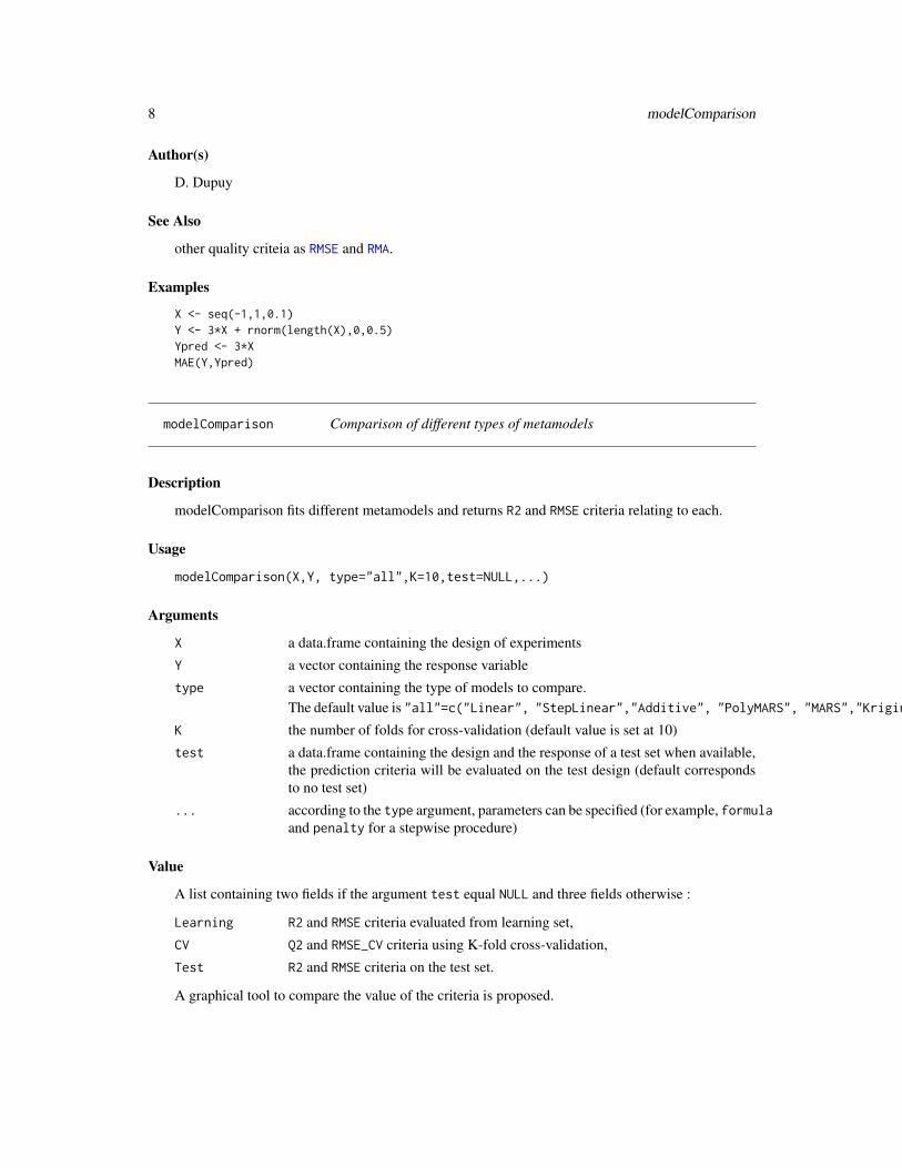
modelComparison Comparison of different types of metamodels

Description

modelComparison fits different metamodels and returns R2 and RMSE criteria relating to each.

Usage

modelComparison(X,Y, type="all",K=10,test=NULL,...)

Arguments

X a data.frame containing the design of experiments

Y a vector containing the response variable

type a vector containing the type of models to compare.The default value is "all"=c("Linear", "StepLinear","Additive", "PolyMARS", "MARS","Kriging")

K the number of folds for cross-validation (default value is set at 10)

test a data.frame containing the design and the response of a test set when available,the prediction criteria will be evaluated on the test design (default correspondsto no test set)

... according to the type argument, parameters can be specified (for example, formulaand penalty for a stepwise procedure)

Value

A list containing two fields if the argument test equal NULL and three fields otherwise :

Learning R2 and RMSE criteria evaluated from learning set,

CV Q2 and RMSE_CV criteria using K-fold cross-validation,

Test R2 and RMSE criteria on the test set.

A graphical tool to compare the value of the criteria is proposed.

modelFit 9

Author(s)

D. Dupuy

See Also

modelFit and crossValidation

Examples

## Not run:data(dataIRSN5D)X <- dataIRSN5D[,1:5]Y <- dataIRSN5D[,6]data(testIRSN5D)library(gam)library(mda)library(polspline)crit <- modelComparison(X,Y, type="all",test=testIRSN5D)

crit2 <- modelComparison(X,Y, type=rep("StepLinear",5),test=testIRSN5D,penalty=c(1,2,5,10,20),formula=Y~.^2)

## End(Not run)

modelFit Fitting metamodels

Description

modelFit is used to fit a metamodel of class lm, gam, mars, polymars or km.

Usage

modelFit (X,Y, type, ...)

Arguments

X a data.frame containing the design of experiments

Y a vector containing the response variable

type represents the method used to fit the model:

"Linear" linear model,"StepLinear" stepwise,"Additive" gam,"MARS" mars"PolyMARS" polymars"Kriging" kriging model.

10 modelFit

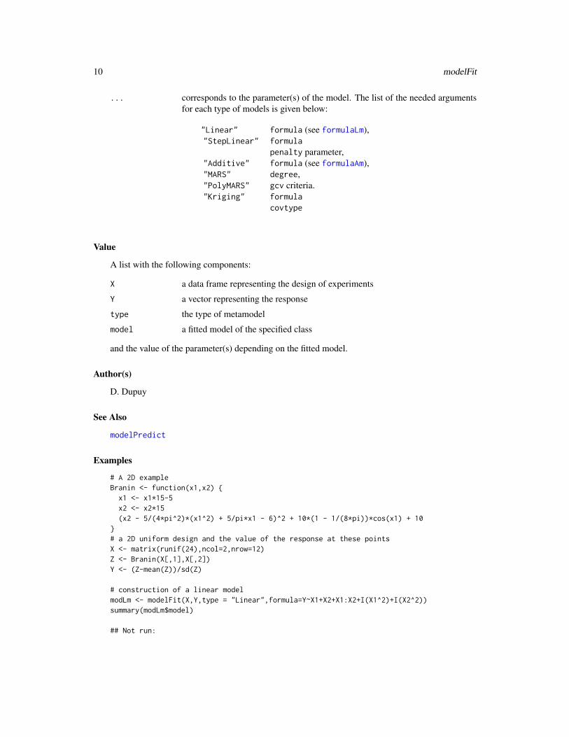
... corresponds to the parameter(s) of the model. The list of the needed argumentsfor each type of models is given below:

"Linear" formula (see formulaLm),"StepLinear" formula

penalty parameter,"Additive" formula (see formulaAm),"MARS" degree,"PolyMARS" gcv criteria."Kriging" formula

covtype

Value

A list with the following components:

X a data frame representing the design of experiments

Y a vector representing the response

type the type of metamodel

model a fitted model of the specified class

and the value of the parameter(s) depending on the fitted model.

Author(s)

D. Dupuy

See Also

modelPredict

Examples

# A 2D exampleBranin <- function(x1,x2) {

x1 <- x1*15-5x2 <- x2*15(x2 - 5/(4*pi^2)*(x1^2) + 5/pi*x1 - 6)^2 + 10*(1 - 1/(8*pi))*cos(x1) + 10

}# a 2D uniform design and the value of the response at these pointsX <- matrix(runif(24),ncol=2,nrow=12)Z <- Branin(X[,1],X[,2])Y <- (Z-mean(Z))/sd(Z)

# construction of a linear modelmodLm <- modelFit(X,Y,type = "Linear",formula=Y~X1+X2+X1:X2+I(X1^2)+I(X2^2))summary(modLm$model)

## Not run:

modelPredict 11

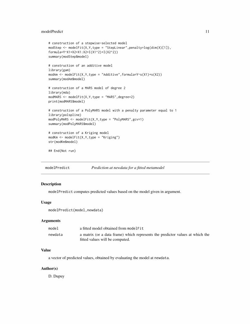
# construction of a stepwise-selected modelmodStep <- modelFit(X,Y,type = "StepLinear",penalty=log(dim(X)[1]),formula=Y~X1+X2+X1:X2+I(X1^2)+I(X2^2))summary(modStep$model)

# construction of an additive modellibrary(gam)modAm <- modelFit(X,Y,type = "Additive",formula=Y~s(X1)+s(X2))summary(modAm$model)

# construction of a MARS model of degree 2library(mda)modMARS <- modelFit(X,Y,type = "MARS",degree=2)print(modMARS$model)

# construction of a PolyMARS model with a penalty parameter equal to 1library(polspline)modPolyMARS <- modelFit(X,Y,type = "PolyMARS",gcv=1)summary(modPolyMARS$model)

# construction of a Kriging modelmodKm <- modelFit(X,Y,type = "Kriging")str(modKm$model)

## End(Not run)

modelPredict Prediction at newdata for a fitted metamodel

Description

modelPredict computes predicted values based on the model given in argument.

Usage

modelPredict(model,newdata)

Arguments

model a fitted model obtained from modelFit

newdata a matrix (or a data frame) which represents the predictor values at which thefitted values will be computed.

Value

a vector of predicted values, obtained by evaluating the model at newdata.

Author(s)

D. Dupuy

12 penaltyPolyMARS

See Also

modelFit

Examples

X <- seq(-1,1,l=21)Y <- 3*X + rnorm(21,0,0.5)# construction of a linear modelmodLm <- modelFit(X,Y,type = "Linear",formula="Y~.")print(modLm$model$coefficient)

## Not run:# illustration on a 2-dimensional exampleBranin <- function(x1,x2) {x1 <- 1/2*(15*x1+5)x2 <- 15/2*(x2+1)(x2 - 5.1/(4*pi^2)*(x1^2) + 5/pi*x1 - 6)^2 + 10*(1 - 1/(8*pi))*cos(x1) + 10}# A 2D uniform design with 20 points in [-1,1]^2n <- 20X <- matrix(runif(n*2,-1,1),ncol=2,nrow=n)Y <- Branin(X[,1],X[,2])Z <- (Y-mean(Y))/sd(Y)

# Construction of a Kriging modelmKm <- modelFit(X,Z,type = "Kriging")

# Prediction and comparison between the exact function and the predicted onextest <- seq(-1, 1, length= 21)ytest <- seq(-1, 1, length= 21)Zreal <- outer(xtest, ytest, Branin)Zreal <- (Zreal-mean(Y))/sd(Y)Zpredict <- modelPredict(mKm,expand.grid(xtest,ytest))

z <- abs(Zreal-matrix(Zpredict,nrow=length(xtest),ncol=length(ytest)))contour(xtest, xtest, z,30)points(X,pch=19)

## End(Not run)

penaltyPolyMARS Choice of the penalty parameter for a PolyMARS model

Description

This function fits a PolyMARS model for different values of the penalty parameter and computecriteria.

penaltyPolyMARS 13

Usage

penaltyPolyMARS(X,Y,test=NULL,graphic=FALSE,K=10,Penalty=seq(0,5,by=0.2))

Arguments

X a data.frame containing the design of experimentsY a vector containing the response variabletest a data.frame containing the design and the response of a test set when available,

the prediction criteria will be computed for the test data (default corresponds tono test set)

graphic if TRUE the values of the criteria are representedK the number of folds for cross-validation (by default, K=10)Penalty a vector containing the values of the penalty parameter

Value

A data frame containing

a the values of the penalty parameterR2 the R2 criterion evaluted on the learning setm the size of the selected model

If a test set is available the last row is

R2test the R2 criterion evaluated on the test set

If no test set is available, criteria computed by K-corss-validation are provided:

Q2 the Q2 evaluated by cross-validation (by default, K=10)RMSE CV RMSE computed by cross-validation

Note that the penalty parameter could be chosen by minimizing the value of the RMSE by cross-validation.

Author(s)

D. Dupuy

See Also

modelFit, R2 and crossValidation

Examples

data(dataIRSN5D)X <- dataIRSN5D[,1:5]Y <- dataIRSN5D[,6]data(testIRSN5D)library(polspline)Crit <- penaltyPolyMARS(X,Y,test=testIRSN5D[,-7],graphic=TRUE)

14 R2

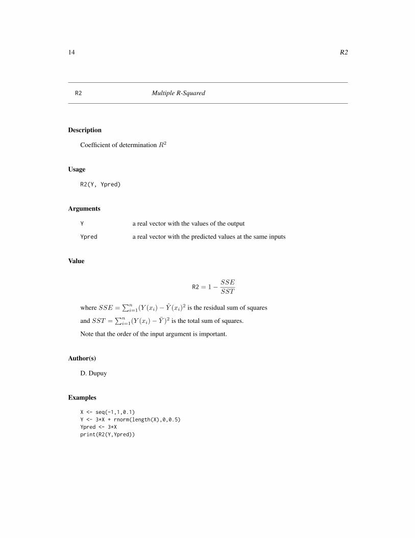
R2 Multiple R-Squared

Description

Coefficient of determination R2

Usage

R2(Y, Ypred)

Arguments

Y a real vector with the values of the output

Ypred a real vector with the predicted values at the same inputs

Value

R2 = 1− SSE

SST

where SSE =∑n

i=1(Y (xi)− Y (xi)2 is the residual sum of squares

and SST =∑n

i=1(Y (xi)− Y )2 is the total sum of squares.

Note that the order of the input argument is important.

Author(s)

D. Dupuy

Examples

X <- seq(-1,1,0.1)Y <- 3*X + rnorm(length(X),0,0.5)Ypred <- 3*Xprint(R2(Y,Ypred))

residualsStudy 15

residualsStudy Plot residuals

Description

residualsStudy analyzes the residuals of a model: a plot of the residuals against the index, a plot ofthe residuals against the fitted values, the representation of the density and a normal Q-Q plot.

Usage

residualsStudy(model)

Arguments

model a fitted model obtained from modelFit

Author(s)

D. Dupuy

See Also

modelFit and modelPredict

Examples

data(dataIRSN5D)X <- dataIRSN5D[,1:5]Y <- dataIRSN5D[,6]library(gam)modAm <- modelFit(X,Y,type = "Additive",formula=formulaAm(X,Y))residualsStudy(modAm)

RMA Relative Maximal Absolute Error

Description

Relative Maximal Absolute Error

Usage

RMA(Y, Ypred)

16 RMA

Arguments

Y a real vector with the values of the output

Ypred a real vector with the predicted values at the same inputs

Value

The RMA criterion represents the maximum of errors between exact values and predicted one:

RMA = max1≤i≤n

|Y (xi)− Y (xi) |σY

where Y is the output variable, Y is the fitted model and σY denotes the standard deviation of Y .

The output of this function is a list with the following components:

max.value the value of the RMA criterion

max.data an integer i indicating the data xi for which the RMA is reached

index a vector containing the data sorted according to the value of the errors

error a vector containing the corresponding value of the errors

Author(s)

D. Dupuy

See Also

other validation criteria as MAE or RMSE.

Examples

X <- seq(-1,1,0.1)Y <- 3*X + rnorm(length(X),0,0.5)Ypred <- 3*Xprint(RMA(Y,Ypred))

# Illustration on Branin functionBranin <- function(x1,x2) {

x1 <- x1*15-5x2 <- x2*15(x2 - 5/(4*pi^2)*(x1^2) + 5/pi*x1 - 6)^2 + 10*(1 - 1/(8*pi))*cos(x1) + 10

}X <- matrix(runif(24),ncol=2,nrow=12)Z <- Branin(X[,1],X[,2])Y <- (Z-mean(Z))/sd(Z)

# Fitting of a Linear model on the data (X,Y)modLm <- modelFit(X,Y,type = "Linear",formula=Y~X1+X2+X1:X2+I(X1^2)+I(X2^2))

# Prediction on a gridu <- seq(0,1,0.1)Y_test_real <- Branin(expand.grid(u,u)[,1],expand.grid(u,u)[,2])

RMSE 17

Y_test_pred <- modelPredict(modLm,expand.grid(u,u))Y_error <- matrix(abs(Y_test_pred-(Y_test_real-mean(Z))/sd(Z)),length(u),length(u))contour(u, u, Y_error,45)Y_pred <- modelPredict(modLm,X)out <- RMA(Y,Y_pred)for (i in 1:dim(X)[1]){

points(X[out$index[i],1],X[out$index[i],2],pch=19,col='red',cex=out$error[i]*10)}

RMSE Root Mean Squared Error

Description

The root of the Mean Squared Error between the exact value and the predicted one.

Usage

RMSE(Y, Ypred)

Arguments

Y a real vector with the values of the output

Ypred a real vector with the predicted values

Value

a real which represents the root of the mean squared error between the target response Y and thefitted one Y :

RMSE =

√√√√ 1

n

n∑i=1

(Y (xi)− Y (xi)

)2.

Author(s)

D. Dupuy

See Also

other validation criteria as MAE or RMA

Examples

X <- seq(-1,1,0.1)Y <- 3*X + rnorm(length(X),0,0.5)Ypred <- 3*Xprint(RMSE(Y,Ypred))

18 stepEvolution

stepEvolution Evolution of the stepwise model

Description

Graphical representation of the selected terms using stepwise procedure for different values of thepenalty parameter.

Usage

stepEvolution(X,Y,formula,P=1:7,K=10,test=NULL,graphic=TRUE)

Arguments

X a data.frame containing the design of experiments

Y a vector containing the response variable

formula a formula for the initial model

P a vector containing different values of the penalty parameter for which a step-wise selected model is fitted

K the number of folds for the cross-validation procedure

test an additional data set on which the prediction criteria are evaluated (default cor-responds to no test data set)

graphic if TRUE the values of the criteria are represented

Value

a list with the different criteria for different values of the penalty parameter. This list contains:

penalty the values for the penalty parameter

m size m of the selected model for each value in P

R2 the value of the R2 criterion for each model

According to the value of the test argument, other criteria are calculated:

a. If a test set is available, R2test contains the value of the R2 criterion on the test setb. If no test set is available, the Q2 and the RMSE computed by cross-validation are done.

Note

Plots are also available. A tabular represents the selected terms for each value in P.

The evolution of the R2 criterion, the evolution of the size m of the selected model and criteria onthe test set or by K-folds cross-validation are represented.

These graphical tools can be used to select the best value for the penalty parameter.

testCrossValidation 19

Author(s)

D. Dupuy

See Also

step procedure for linear models.

Examples

## Not run:data(dataIRSN5D)design <- dataIRSN5D[,1:5]Y <- dataIRSN5D[,6]out <- stepEvolution(design,Y,formulaLm(design,Y),P=c(1,2,5,10,20,30))

## End(Not run)

testCrossValidation Test the robustess of the cross-validation procedure

Description

This function calculates the estimated K-fold cross-validation for different values of K.

Usage

testCrossValidation(model,Kfold=c(2,5,10,20,30,40,dim(model$data$X)[1]),N=10)

Arguments

model a fitted model from modelFit

Kfold a vector containing the values to test (default corresponds to 2,5,10,20,30,40 andthe number of observations for leave-one-out procedure)

N an integer given the number of times the K-fold cross-validation is performedfor each value of K

Value

a matrix of all the values obtained by K-fold cross-validation

Note

For each value of K, the cross-validation procedure is repeated N times in order to get an idea of thedispersion of the Q2 criterion and of the RMSE by K-fold cross-validation.

Author(s)

D. Dupuy

20 testIRSN5D

See Also

crossValidation

Examples

## Not run:rm(list=ls())# A 2D exampleBranin <- function(x1,x2) {

x1 <- x1*15-5x2 <- x2*15(x2 - 5/(4*pi^2)*(x1^2) + 5/pi*x1 - 6)^2 + 10*(1 - 1/(8*pi))*cos(x1) + 10

}# a 2D uniform design and the value of the response at these pointsn <- 50X <- matrix(runif(n*2),ncol=2,nrow=n)Y <- Branin(X[,1],X[,2])

mod <- modelFit(X,Y,type="Linear",formula=formulaLm(X,Y))out <- testCrossValidation(mod,N=20)

## End(Not run)

testIRSN5D A set of test data

Description

These test data correspond to the five-dimensional case provided by the IRSN detailed in dataIRSN5D.

Usage

data(testIRSN5D)

Format

A data frame with 324 rows representing the number of observations and 6 columns: the first fivecorresponding to the input variables ("b","e","p","r" and "l") and the last to the response Keff.

Source

IRSN (Institut de Radioprotection et de Sûreté Nucléaire)

See Also

dataIRSN5D

Index

∗Topic datasetsdataIRSN5D, 6testIRSN5D, 20

∗Topic modelscrossValidation, 4DiceEval-package, 2MAE, 7modelComparison, 8modelFit, 9modelPredict, 11penaltyPolyMARS, 12R2, 14residualsStudy, 15RMA, 15RMSE, 17stepEvolution, 18testCrossValidation, 19

∗Topic packageDiceEval-package, 2

crossValidation, 3, 4, 9, 13, 20

dataIRSN5D, 6, 20DiceEval (DiceEval-package), 2DiceEval-package, 2

foldsComposition, 5formulaAm, 10formulaLm, 10

gam, 2

km, 2

MAE, 4, 5, 7, 16, 17mars, 2modelComparison, 3, 8modelFit, 3, 5, 9, 9, 12, 13, 15modelPredict, 3, 10, 11, 15

penaltyPolyMARS, 12

polymars, 2

R2, 5, 13, 14residualsStudy, 15RMA, 8, 15, 17RMSE, 4, 5, 8, 16, 17

stepEvolution, 18

testCrossValidation, 5, 19testIRSN5D, 20

21