Package ‘corpcor’ - The Comprehensive R Archive Network · PDF filePackage...
27
Package ‘corpcor’ April 1, 2017 Version 1.6.9 Date 2017-03-31 Title Efficient Estimation of Covariance and (Partial) Correlation Author Juliane Schafer, Rainer Opgen-Rhein, Verena Zuber, Miika Ahdesmaki, A. Pedro Duarte Silva, and Korbinian Strimmer. Maintainer Korbinian Strimmer <[email protected]> Depends R (>= 3.0.2) Imports stats Suggests Description Implements a James-Stein-type shrinkage estimator for the covariance matrix, with separate shrinkage for variances and correlations. The details of the method are explained in Schafer and Strimmer (2005) <DOI:10.2202/1544-6115.1175> and Opgen-Rhein and Strimmer (2007) <DOI:10.2202/1544-6115.1252>. The approach is both computationally as well as statistically very efficient, it is applicable to ``small n, large p'' data, and always returns a positive definite and well-conditioned covariance matrix. In addition to inferring the covariance matrix the package also provides shrinkage estimators for partial correlations and partial variances. The inverse of the covariance and correlation matrix can be efficiently computed, as well as any arbitrary power of the shrinkage correlation matrix. Furthermore, functions are available for fast singular value decomposition, for computing the pseudoinverse, and for checking the rank and positive definiteness of a matrix. License GPL (>= 3) URL http://strimmerlab.org/software/corpcor/ NeedsCompilation no Repository CRAN Date/Publication 2017-04-01 06:30:37 UTC 1
Transcript of Package ‘corpcor’ - The Comprehensive R Archive Network · PDF filePackage...
Package ‘corpcor’April 1, 2017
Version 1.6.9
Date 2017-03-31
Title Efficient Estimation of Covariance and (Partial) Correlation
Author Juliane Schafer, Rainer Opgen-Rhein, Verena Zuber, Miika Ahdesmaki,A. Pedro Duarte Silva, and Korbinian Strimmer.
Maintainer Korbinian Strimmer <[email protected]>
Depends R (>= 3.0.2)
Imports stats
Suggests
Description Implements a James-Stein-type shrinkage estimator forthe covariance matrix, with separate shrinkage for variances and correlations.The details of the method are explained in Schafer and Strimmer (2005)<DOI:10.2202/1544-6115.1175> and Opgen-Rhein and Strimmer (2007)<DOI:10.2202/1544-6115.1252>. The approach is both computationally as wellas statistically very efficient, it is applicable to ``small n, large p'' data,and always returns a positive definite and well-conditioned covariance matrix.In addition to inferring the covariance matrix the package also providesshrinkage estimators for partial correlations and partial variances.The inverse of the covariance and correlation matrixcan be efficiently computed, as well as any arbitrary power of theshrinkage correlation matrix. Furthermore, functions are available for fastsingular value decomposition, for computing the pseudoinverse, and forchecking the rank and positive definiteness of a matrix.
License GPL (>= 3)
URL http://strimmerlab.org/software/corpcor/
NeedsCompilation no
Repository CRAN
Date/Publication 2017-04-01 06:30:37 UTC
1
2 corpcor-package
R topics documented:corpcor-package . . . . . . . . . . . . . . . . . . . . . . . . . . . . . . . . . . . . . . . 2cor2pcor . . . . . . . . . . . . . . . . . . . . . . . . . . . . . . . . . . . . . . . . . . . 3cov.shrink . . . . . . . . . . . . . . . . . . . . . . . . . . . . . . . . . . . . . . . . . . 4fast.svd . . . . . . . . . . . . . . . . . . . . . . . . . . . . . . . . . . . . . . . . . . . 7invcov.shrink . . . . . . . . . . . . . . . . . . . . . . . . . . . . . . . . . . . . . . . . 9mpower . . . . . . . . . . . . . . . . . . . . . . . . . . . . . . . . . . . . . . . . . . . 11pcor.shrink . . . . . . . . . . . . . . . . . . . . . . . . . . . . . . . . . . . . . . . . . 12powcor.shrink . . . . . . . . . . . . . . . . . . . . . . . . . . . . . . . . . . . . . . . . 14pseudoinverse . . . . . . . . . . . . . . . . . . . . . . . . . . . . . . . . . . . . . . . . 17rank.condition . . . . . . . . . . . . . . . . . . . . . . . . . . . . . . . . . . . . . . . . 19rebuild.cov . . . . . . . . . . . . . . . . . . . . . . . . . . . . . . . . . . . . . . . . . 20shrink.intensity . . . . . . . . . . . . . . . . . . . . . . . . . . . . . . . . . . . . . . . 22smtools . . . . . . . . . . . . . . . . . . . . . . . . . . . . . . . . . . . . . . . . . . . 24wt.scale . . . . . . . . . . . . . . . . . . . . . . . . . . . . . . . . . . . . . . . . . . . 25
Index 27
corpcor-package The corpcor Package
Description
This package implements a James-Stein-type shrinkage estimator for the covariance matrix, withseparate shrinkage for variances and correlations. The details of the method are explained inSch\"afer and Strimmer (2005) <DOI:10.2202/1544-6115.1175> and Opgen-Rhein and Strimmer(2007) <DOI:10.2202/1544-6115.1252>. The approach is both computationally as well as statisti-cally very efficient, it is applicable to “small n, large p” data, and always returns a positive definiteand well-conditioned covariance matrix. In addition to inferring the covariance matrix the packagealso provides shrinkage estimators for partial correlations, partial variances, and regression coeffi-cients. The inverse of the covariance and correlation matrix can be efficiently computed, and as wellas any arbitrary power of the shrinkage correlation matrix. Furthermore, functions are available forfast singular value decomposition, for computing the pseudoinverse, and for checking the rank andpositive definiteness of a matrix.
The name of the package refers to correlations and partial correlations.
Author(s)
Juliane Sch\"afer, Rainer Opgen-Rhein, Verena Zuber, Miika Ahdesm\"aki, A. Pedro Duarte Silva,and Korbinian Strimmer (http://strimmerlab.org/)
References
See website: http://strimmerlab.org/software/corpcor/
See Also
cov.shrink, invcov.shrink, powcor.shrink, pcor.shrink, fast.svd.

cor2pcor 3
cor2pcor Compute Partial Correlation from Correlation Matrix – and ViceVersa
Description
cor2pcor computes the pairwise partial correlation coefficients from either a correlation or a co-variance matrix.
pcor2cor takes either a partial correlation matrix or a partial covariance matrix as input, and com-putes from it the corresponding correlation matrix.
Usage
cor2pcor(m, tol)pcor2cor(m, tol)
Arguments
m covariance matrix or (partial) correlation matrix
tol tolerance - singular values larger than tol are considered non-zero (default value:tol = max(dim(m))*max(D)*.Machine$double.eps). This parameter is neededfor the singular value decomposition on which pseudoinverse is based.
Details
The partial correlations are the negative standardized concentrations (which in turn are the off-diagonal elements of the inverse correlation or covariance matrix). In graphical Gaussian modelsthe partial correlations represent the direct interactions between two variables, conditioned on allremaining variables.
In the above functions the pseudoinverse is employed for inversion - hence even singular covari-ances (with some zero eigenvalues) may be used. However, a better option may be to estimate apositive definite covariance matrix using cov.shrink.
Note that for efficient computation of partial correlation coefficients from data x it is advised to usepcor.shrink(x) and not cor2pcor(cor.shrink(x)).
Value
A matrix with the pairwise partial correlation coefficients (cor2pcor) or with pairwise correlations(pcor2cor).
Author(s)
Korbinian Strimmer (http://strimmerlab.org).
References
Whittaker J. 1990. Graphical Models in Applied Multivariate Statistics. John Wiley, Chichester.

4 cov.shrink
See Also
decompose.invcov, pcor.shrink, pseudoinverse.
Examples
# load corpcor librarylibrary("corpcor")
# covariance matrixm.cov = rbind(c(3,1,1,0),c(1,3,0,1),c(1,0,2,0),c(0,1,0,2)
)m.cov
# corresponding correlation matrixm.cor.1 = cov2cor(m.cov)m.cor.1
# compute partial correlations (from covariance matrix)m.pcor.1 = cor2pcor(m.cov)m.pcor.1
# compute partial correlations (from correlation matrix)m.pcor.2 = cor2pcor(m.cor.1)m.pcor.2
zapsmall( m.pcor.1 ) == zapsmall( m.pcor.2 )
# backtransformationm.cor.2 = pcor2cor(m.pcor.1)m.cor.2zapsmall( m.cor.1 ) == zapsmall( m.cor.2 )
cov.shrink Shrinkage Estimates of Covariance and Correlation
Description
The functions var.shrink, cor.shrink, and cov.shrink compute shrinkage estimates of vari-ance, correlation, and covariance, respectively.
cov.shrink 5
Usage
var.shrink(x, lambda.var, w, verbose=TRUE)cor.shrink(x, lambda, w, verbose=TRUE)cov.shrink(x, lambda, lambda.var, w, verbose=TRUE)
Arguments
x a data matrixlambda the correlation shrinkage intensity (range 0-1). If lambda is not specified (the
default) it is estimated using an analytic formula from Sch\"afer and Strimmer(2005) - see details below. For lambda=0 the empirical correlations are recov-ered.
lambda.var the variance shrinkage intensity (range 0-1). If lambda.var is not specified(the default) it is estimated using an analytic formula from Opgen-Rhein andStrimmer (2007) - see details below. For lambda.var=0 the empirical variancesare recovered.
w optional: weights for each data point - if not specified uniform weights are as-sumed (w = rep(1/n, n) with n = nrow(x)).
verbose output some status messages while computing (default: TRUE)
Details
var.shrink computes the empirical variance of each considered random variable, and shrinks themtowards their median. The shrinkage intensity is estimated using estimate.lambda.var (Opgen-Rhein and Strimmer 2007).
Similarly cor.shrink computes a shrinkage estimate of the correlation matrix by shrinking theempirical correlations towards the identity matrix. In this case the shrinkage intensity is computedusing estimate.lambda (Sch\"afer and Strimmer 2005).
In comparison with the standard empirical estimates (var, cov, and cor) the shrinkage estimatesexhibit a number of favorable properties. For instance,
1. they are typically much more efficient, i.e. they show (sometimes dramatically) better meansquared error,
2. the estimated covariance and correlation matrices are always positive definite and well condi-tioned (so that there are no numerical problems when computing their inverse),
3. they are inexpensive to compute, and4. they are fully automatic and do not require any tuning parameters (as the shrinkage intensity
is analytically estimated from the data), and5. they assume nothing about the underlying distributions, except for the existence of the first
two moments.
These properties also carry over to derived quantities, such as partial variances and partial correla-tions (pvar.shrink and pcor.shrink).
As an extra benefit, the shrinkage estimators have a form that can be very efficiently inverted,especially if the number of variables is large and the sample size is small. Thus, instead of invertingthe matrix output by cov.shrink and cor.shrink please use the functions invcov.shrink andinvcor.shrink, respectively.

6 cov.shrink
Value
var.shrink returns a vector with estimated variances.
cov.shrink returns a covariance matrix.
cor.shrink returns the corresponding correlation matrix.
Author(s)
Juliane Sch\"afer, Rainer Opgen-Rhein, and Korbinian Strimmer (http://strimmerlab.org).
References
Opgen-Rhein, R., and K. Strimmer. 2007. Accurate ranking of differentially expressed genes by adistribution-free shrinkage approach. Statist. Appl. Genet. Mol. Biol. 6:9. <DOI:10.2202/1544-6115.1252>
Sch\"afer, J., and K. Strimmer. 2005. A shrinkage approach to large-scale covariance estimation andimplications for functional genomics. Statist. Appl. Genet. Mol. Biol. 4:32. <DOI:10.2202/1544-6115.1175>
See Also
invcov.shrink, pcor.shrink, cor2pcor
Examples
# load corpcor librarylibrary("corpcor")
# small n, large pp = 100n = 20
# generate random pxp covariance matrixsigma = matrix(rnorm(p*p),ncol=p)sigma = crossprod(sigma)+ diag(rep(0.1, p))
# simulate multinormal data of sample size nsigsvd = svd(sigma)Y = t(sigsvd$v %*% (t(sigsvd$u) * sqrt(sigsvd$d)))X = matrix(rnorm(n * ncol(sigma)), nrow = n) %*% Y
# estimate covariance matrixs1 = cov(X)s2 = cov.shrink(X)
# squared errorsum((s1-sigma)^2)sum((s2-sigma)^2)
fast.svd 7
# compare positive definitenessis.positive.definite(sigma)is.positive.definite(s1)is.positive.definite(s2)
# compare ranks and conditionrank.condition(sigma)rank.condition(s1)rank.condition(s2)
# compare eigenvaluese0 = eigen(sigma, symmetric=TRUE)$valuese1 = eigen(s1, symmetric=TRUE)$valuese2 = eigen(s2, symmetric=TRUE)$valuesm = max(e0, e1, e2)yl = c(0, m)
par(mfrow=c(1,3))plot(e1, main="empirical")plot(e2, ylim=yl, main="full shrinkage")plot(e0, ylim=yl, main="true")par(mfrow=c(1,1))
fast.svd Fast Singular Value Decomposition
Description
fast.svd returns the singular value decomposition of a rectangular real matrix
M = UDV′,
where U and V are orthogonal matrices with U ′U = I and V ′V = I , and D is a diagonal matrixcontaining the singular values (see svd).
The main difference to the native version svd is that fast.svd is substantially faster for "fat" (smalln, large p) and "thin" (large n, small p) matrices. In this case the decomposition ofM can be greatlysped up by first computing the SVD of either MM ′ (fat matrices) or M ′M (thin matrices), ratherthan that of M .
A second difference to svd is that fast.svd only returns the positive singular values (thus thedimension ofD always equals the rank ofM ). Note that the singular vectors computed by fast.svdmay differ in sign from those computed by svd.
Usage
fast.svd(m, tol)
8 fast.svd
Arguments
m matrix
tol tolerance - singular values larger than tol are considered non-zero (default value:tol = max(dim(m))*max(D)*.Machine$double.eps)
Details
For "fat" M (small n, large p) the SVD decomposition of MM ′ yields
MM′= UD2U
As the matrix MM ′ has dimension n x n only, this is faster to compute than SVD of M . The Vmatrix is subsequently obtained by
V =M′UD−1
Similarly, for "thin" M (large n, small p), the decomposition of M ′M yields
M′M = V D2V
′
which is also quick to compute as M ′M has only dimension p x p. The U matrix is then computedvia
U =MVD−1
Value
A list with the following components:
d a vector containing the positive singular values
u a matrix with the corresponding left singular vectors
v a matrix with the corresponding right singular vectors
Author(s)
Korbinian Strimmer (http://strimmerlab.org).
See Also
svd, solve.
invcov.shrink 9
Examples
# load corpcor librarylibrary("corpcor")
# generate a "fat" data matrixn = 50p = 5000X = matrix(rnorm(n*p), n, p)
# compute SVDsystem.time( (s1 = svd(X)) )system.time( (s2 = fast.svd(X)) )
eps = 1e-10sum(abs(s1$d-s2$d) > eps)sum(abs(abs(s1$u)-abs(s2$u)) > eps)sum(abs(abs(s1$v)-abs(s2$v)) > eps)
invcov.shrink Fast Computation of the Inverse of the Covariance and CorrelationMatrix
Description
The functions invcov.shrink and invcor.shrink implement an algorithm to efficiently computethe inverses of shrinkage estimates of covariance (cov.shrink) and correlation (cor.shrink).
Usage
invcov.shrink(x, lambda, lambda.var, w, verbose=TRUE)invcor.shrink(x, lambda, w, verbose=TRUE)
Arguments
x a data matrixlambda the correlation shrinkage intensity (range 0-1). If lambda is not specified (the
default) it is estimated using an analytic formula from Sch\"afer and Strimmer(2005) - see cor.shrink. For lambda=0 the empirical correlations are recov-ered.
lambda.var the variance shrinkage intensity (range 0-1). If lambda.var is not specified (thedefault) it is estimated using an analytic formula from Sch\"afer and Strimmer(2005) - see var.shrink. For lambda.var=0 the empirical variances are recov-ered.
w optional: weights for each data point - if not specified uniform weights are as-sumed (w = rep(1/n, n) with n = nrow(x)).
verbose output status while computing (default: TRUE)
10 invcov.shrink
Details
Both invcov.shrink and invcor.shrink rely on powcor.shrink. This allows to compute theinverses in a very efficient fashion (much more efficient than directly inverting the matrices - seethe example).
Value
invcov.shrink returns the inverse of the output from cov.shrink.
invcor.shrink returns the inverse of the output from cor.shrink.
Author(s)
Juliane Sch\"afer and Korbinian Strimmer (http://strimmerlab.org).
References
Sch\"afer, J., and K. Strimmer. 2005. A shrinkage approach to large-scale covariance estimation andimplications for functional genomics. Statist. Appl. Genet. Mol. Biol. 4:32. <DOI:10.2202/1544-6115.1175>
See Also
powcor.shrink, cov.shrink, pcor.shrink, cor2pcor
Examples
# load corpcor librarylibrary("corpcor")
# generate data matrixp = 500n = 10X = matrix(rnorm(n*p), nrow = n, ncol = p)
lambda = 0.23 # some arbitrary lambda
# slowsystem.time(
(W1 = solve(cov.shrink(X, lambda))))
# very fastsystem.time(
(W2 = invcov.shrink(X, lambda)))
# no differencesum((W1-W2)^2)
mpower 11
mpower Compute the Power of a Real Symmetric Matrix
Description
mpower computes malpha, i.e. the alpha-th power of the real symmetric matrix m.
Usage
mpower(m, alpha, pseudo=FALSE, tol)
Arguments
m a real-valued symmetric matrix.
alpha exponent.
pseudo if pseudo=TRUE then all zero eigenvalues are dropped (e.g. for computing thepseudoinverse). The default is to use all eigenvalues.
tol tolerance - eigenvalues with absolute value smaller or equal to tol are consid-ered identically zero (default: tol = max(dim(m))*max(abs(eval))*.Machine$double.eps).
Details
The matrix power of m is obtained by first computing the spectral decomposition of m, and subse-quent modification of the resulting eigenvalues.
Note that m is assumed to by symmetric, and only its lower triangle (diagonal included) is used ineigen.
For computing the matrix power of cor.shrink use the vastly more efficient function powcor.shrink.
Value
mpower returns a matrix of the same dimensions as m.
Author(s)
Korbinian Strimmer (http://strimmerlab.org).
See Also
powcor.shrink, eigen.
12 pcor.shrink
Examples
# load corpcor librarylibrary("corpcor")
# generate symmetric matrixp = 10n = 20X = matrix(rnorm(n*p), nrow = n, ncol = p)m = cor(X)
m %*% mmpower(m, 2)
solve(m)mpower(m, -1)
msq = mpower(m, 0.5)msq %*% msqm
mpower(m, 1.234)
pcor.shrink Shrinkage Estimates of Partial Correlation and Partial Variance
Description
The functions pcor.shrink and pvar.shrink compute shrinkage estimates of partial correlationand partial variance, respectively.
Usage
pcor.shrink(x, lambda, w, verbose=TRUE)pvar.shrink(x, lambda, lambda.var, w, verbose=TRUE)
Arguments
x a data matrixlambda the correlation shrinkage intensity (range 0-1). If lambda is not specified (the
default) it is estimated using an analytic formula from Sch\"afer and Strimmer(2005) - see cor.shrink. For lambda=0 the empirical correlations are recov-ered.
lambda.var the variance shrinkage intensity (range 0-1). If lambda.var is not specified(the default) it is estimated using an analytic formula from Opgen-Rhein andStrimmer (2007) - see details below. For lambda.var=0 the empirical variancesare recovered.
w optional: weights for each data point - if not specified uniform weights are as-sumed (w = rep(1/n, n) with n = nrow(x)).
verbose report progress while computing (default: TRUE)
pcor.shrink 13
Details
The partial variance var(Xk|rest) is the variance of Xk conditioned on the remaining variables. Itequals the inverse of the corresponding diagonal entry of the precision matrix (see Whittaker 1990).
The partial correlations corr(Xk, Xl|rest) is the correlation betweenXk andXl conditioned on theremaining variables. It equals the sign-reversed entries of the off-diagonal entries of the precisionmatrix, standardized by the the squared root of the associated inverse partial variances.
Note that using pcor.shrink(x) much faster than cor2pcor(cor.shrink(x)).
For details about the shrinkage procedure consult Sch\"afer and Strimmer (2005), Opgen-Rhein andStrimmer (2007), and the help page of cov.shrink.
Value
pcor.shrink returns the partial correlation matrix. Attached to this matrix are the standardizedpartial variances (i.e. PVAR/VAR) that can be retrieved using attr under the attribute "spv".
pvar.shrink returns the partial variances.
Author(s)
Juliane Sch\"afer and Korbinian Strimmer (http://strimmerlab.org).
References
Opgen-Rhein, R., and K. Strimmer. 2007. Accurate ranking of differentially expressed genes by adistribution-free shrinkage approach. Statist. Appl. Genet. Mol. Biol. 6:9. <DOI:10.2202/1544-6115.1252>
Sch\"afer, J., and K. Strimmer. 2005. A shrinkage approach to large-scale covariance estimation andimplications for functional genomics. Statist. Appl. Genet. Mol. Biol. 4:32. <DOI:10.2202/1544-6115.1175>
Whittaker J. 1990. Graphical Models in Applied Multivariate Statistics. John Wiley, Chichester.
See Also
invcov.shrink, cov.shrink, cor2pcor
Examples
# load corpcor librarylibrary("corpcor")
# generate data matrixp = 50n = 10X = matrix(rnorm(n*p), nrow = n, ncol = p)
# partial variancepv = pvar.shrink(X)pv
14 powcor.shrink
# partial correlations (fast and recommend way)pcr1 = pcor.shrink(X)
# other possibilities to estimate partial correlationspcr2 = cor2pcor( cor.shrink(X) )
# all the samesum((pcr1 - pcr2)^2)
powcor.shrink Fast Computation of the Power of the Shrinkage Correlation Matrix
Description
The function powcor.shrink efficiently computes the alpha-th power of the shrinkage correlationmatrix produced by cor.shrink.
For instance, this function may be used for fast computation of the (inverse) square root of theshrinkage correlation matrix (needed, e.g., for decorrelation).
crossprod.powcor.shrink efficiently computes Rαy without actually computing the full matrixRα.
Usage
powcor.shrink(x, alpha, lambda, w, verbose=TRUE)crossprod.powcor.shrink(x, y, alpha, lambda, w, verbose=TRUE)
Arguments
x a data matrix
y a matrix, the number of rows of y must be the same as the number of columnsof x
alpha exponent
lambda the correlation shrinkage intensity (range 0-1). If lambda is not specified (thedefault) it is estimated using an analytic formula from Sch\"afer and Strimmer(2005) - see cor.shrink. For lambda=0 the empirical correlations are recov-ered.
w optional: weights for each data point - if not specified uniform weights are as-sumed (w = rep(1/n, n) with n = nrow(x)).
verbose output status while computing (default: TRUE)
powcor.shrink 15
Details
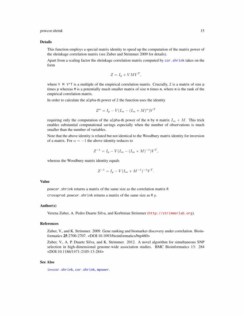
This function employs a special matrix identity to speed up the computation of the matrix power ofthe shrinkage correlation matrix (see Zuber and Strimmer 2009 for details).
Apart from a scaling factor the shrinkage correlation matrix computed by cor.shrink takes on theform
Z = Ip + VMV T ,
where V M V^T is a multiple of the empirical correlation matrix. Crucially, Z is a matrix of size ptimes p whereas M is a potentially much smaller matrix of size m times m, where m is the rank of theempirical correlation matrix.
In order to calculate the alpha-th power of Z the function uses the identity
Zα = Ip − V (Im − (Im +M)α)V T
requiring only the computation of the alpha-th power of the m by m matrix Im +M . This trickenables substantial computational savings especially when the number of observations is muchsmaller than the number of variables.
Note that the above identity is related but not identical to the Woodbury matrix identity for inversionof a matrix. For α = −1 the above identity reduces to
Z−1 = Ip − V (Im − (Im +M)−1)V T ,
whereas the Woodbury matrix identity equals
Z−1 = Ip − V (Im +M−1)−1V T .
Value
powcor.shrink returns a matrix of the same size as the correlation matrix R
crossprod.powcor.shrink returns a matrix of the same size as R y.
Author(s)
Verena Zuber, A. Pedro Duarte Silva, and Korbinian Strimmer (http://strimmerlab.org).
References
Zuber, V., and K. Strimmer. 2009. Gene ranking and biomarker discovery under correlation. Bioin-formatics 25:2700-2707. <DOI:10.1093/bioinformatics/btp460>
Zuber, V., A. P. Duarte Silva, and K. Strimmer. 2012. A novel algorithm for simultaneous SNPselection in high-dimensional genome-wide association studies. BMC Bioinformatics 13: 284<DOI:10.1186/1471-2105-13-284>
See Also
invcor.shrink, cor.shrink, mpower.
16 powcor.shrink
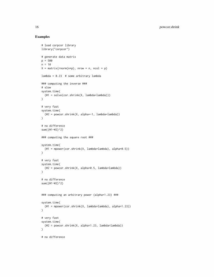
Examples
# load corpcor librarylibrary("corpcor")
# generate data matrixp = 500n = 10X = matrix(rnorm(n*p), nrow = n, ncol = p)
lambda = 0.23 # some arbitrary lambda
### computing the inverse #### slowsystem.time(
(W1 = solve(cor.shrink(X, lambda=lambda))))
# very fastsystem.time(
(W2 = powcor.shrink(X, alpha=-1, lambda=lambda)))
# no differencesum((W1-W2)^2)
### computing the square root ###
system.time((W1 = mpower(cor.shrink(X, lambda=lambda), alpha=0.5))
)
# very fastsystem.time(
(W2 = powcor.shrink(X, alpha=0.5, lambda=lambda)))
# no differencesum((W1-W2)^2)
### computing an arbitrary power (alpha=1.23) ###
system.time((W1 = mpower(cor.shrink(X, lambda=lambda), alpha=1.23))
)
# very fastsystem.time(
(W2 = powcor.shrink(X, alpha=1.23, lambda=lambda)))
# no difference
pseudoinverse 17
sum((W1-W2)^2)
### fast computation of cross product
y = rnorm(p)
system.time((CP1 = crossprod(powcor.shrink(X, alpha=1.23, lambda=lambda), y))
)
system.time((CP2 = crossprod.powcor.shrink(X, y, alpha=1.23, lambda=lambda))
)
# no differencesum((CP1-CP2)^2)
pseudoinverse Pseudoinverse of a Matrix
Description
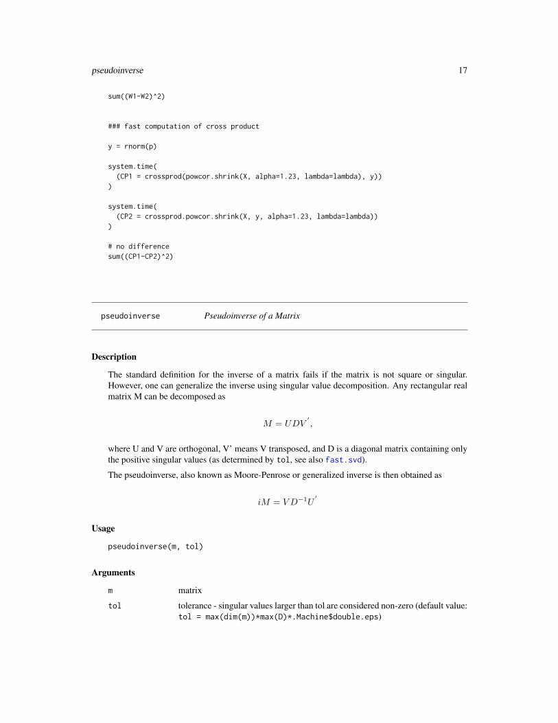
The standard definition for the inverse of a matrix fails if the matrix is not square or singular.However, one can generalize the inverse using singular value decomposition. Any rectangular realmatrix M can be decomposed as
M = UDV′,
where U and V are orthogonal, V’ means V transposed, and D is a diagonal matrix containing onlythe positive singular values (as determined by tol, see also fast.svd).
The pseudoinverse, also known as Moore-Penrose or generalized inverse is then obtained as
iM = V D−1U′
Usage
pseudoinverse(m, tol)
Arguments
m matrix
tol tolerance - singular values larger than tol are considered non-zero (default value:tol = max(dim(m))*max(D)*.Machine$double.eps)

18 pseudoinverse
Details
The pseudoinverse has the property that the sum of the squares of all the entries in iM %*% M - I,where I is an appropriate identity matrix, is minimized. For non-singular matrices the pseudoinverseis equivalent to the standard inverse.
Value
A matrix (the pseudoinverse of m).
Author(s)
Korbinian Strimmer (http://strimmerlab.org).
See Also
solve, fast.svd
Examples
# load corpcor librarylibrary("corpcor")
# a singular matrixm = rbind(c(1,2),c(1,2))
# not possible to invert exactlytry(solve(m))
# pseudoinversep = pseudoinverse(m)p
# characteristics of the pseudoinversezapsmall( m %*% p %*% m ) == zapsmall( m )zapsmall( p %*% m %*% p ) == zapsmall( p )zapsmall( p %*% m ) == zapsmall( t(p %*% m ) )zapsmall( m %*% p ) == zapsmall( t(m %*% p ) )
# example with an invertable matrixm2 = rbind(c(1,1),c(1,0))zapsmall( solve(m2) ) == zapsmall( pseudoinverse(m2) )

rank.condition 19
rank.condition Positive Definiteness of a Matrix, Rank and Condition Number
Description
is.positive.definite tests whether all eigenvalues of a symmetric matrix are positive.
make.positive.definite computes the nearest positive definite of a real symmetric matrix, usingthe algorithm of NJ Higham (1988) <DOI:10.1016/0024-3795(88)90223-6>.
rank.condition estimates the rank and the condition of a matrix by computing its singular valuesD[i] (using svd). The rank of the matrix is the number of singular values D[i] > tol) and thecondition is the ratio of the largest and the smallest singular value.
The definition tol= max(dim(m))*max(D)*.Machine$double.eps is exactly compatible with theconventions used in "Octave" or "Matlab".
Also note that it is not checked whether the input matrix m is real and symmetric.
Usage
is.positive.definite(m, tol, method=c("eigen", "chol"))make.positive.definite(m, tol)rank.condition(m, tol)
Arguments
m a matrix (assumed to be real and symmetric)
tol tolerance for singular values and for absolute eigenvalues - only those with val-ues larger than tol are considered non-zero (default: tol = max(dim(m))*max(D)*.Machine$double.eps)
method Determines the method to check for positive definiteness: eigenvalue computa-tion (eigen, default) or Cholesky decomposition (chol).
Value
is.positive.definite returns a logical value (TRUE or FALSE).
rank.condition returns a list object with the following components:
rank Rank of the matrix.
condition Condition number.
tol Tolerance.
make.positive.definite returns a symmetric positive definite matrix.
Author(s)
Korbinian Strimmer (http://strimmerlab.org).

20 rebuild.cov
See Also
svd, pseudoinverse.
Examples
# load corpcor librarylibrary("corpcor")
# Hilbert matrixhilbert = function(n) { i = 1:n; 1 / outer(i - 1, i, "+") }
# positive definite ?m = hilbert(8)is.positive.definite(m)
# numerically ill-conditionedm = hilbert(15)rank.condition(m)
# make positive definitem2 = make.positive.definite(m)is.positive.definite(m2)rank.condition(m2)m2 - m
rebuild.cov Rebuild and Decompose the (Inverse) Covariance Matrix
Description
rebuild.cov takes a correlation matrix and a vector with variances and reconstructs the corre-sponding covariance matrix.
Conversely, decompose.cov decomposes a covariance matrix into correlations and variances.
decompose.invcov decomposes a concentration matrix (=inverse covariance matrix) into partialcorrelations and partial variances.
rebuild.invcov takes a partial correlation matrix and a vector with partial variances and recon-structs the corresponding concentration matrix.
Usage
rebuild.cov(r, v)rebuild.invcov(pr, pv)decompose.cov(m)decompose.invcov(m)

rebuild.cov 21
Arguments
r correlation matrix
v variance vector
pr partial correlation matrix
pv partial variance vector
m a covariance or a concentration matrix
Details
The diagonal elements of the concentration matrix (=inverse covariance matrix) are the precisions,and the off-diagonal elements are the concentrations. Thus, the partial variances correspond to theinverse precisions, and the partial correlations to the negative standardized concentrations.
Value
rebuild.cov and rebuild.invcov return a matrix.
decompose.cov and decompose.invcov return a list containing a matrix and a vector.
Author(s)
Korbinian Strimmer (http://strimmerlab.org).
See Also
cor, cov, pcor.shrink
Examples
# load corpcor librarylibrary("corpcor")
# a correlation matrix and some variancesr = matrix(c(1, 1/2, 1/2, 1), nrow = 2, ncol=2)rv = c(2, 3)
# construct the associated covariance matrixc = rebuild.cov(r, v)c
# decompose into correlations and variancesdecompose.cov(c)
# the corresponding concentration matrixconc = pseudoinverse(c)conc
# decompose into partial correlation matrix and partial variances

22 shrink.intensity
tmp = decompose.invcov(conc)tmp# note: because this is an example with two variables,# the partial and standard correlations are identical!
# reconstruct the concentration matrix from partial correlations and# partial variancesrebuild.invcov(tmp$pr, tmp$pv)
shrink.intensity Estimation of Shrinkage Intensities
Description
The functions estimate.lambda and estimate.lambda.var shrinkage intensities used for corre-lations and variances used in cor.shrink and var.shrink, respectively.
Usage
estimate.lambda(x, w, verbose=TRUE)estimate.lambda.var(x, w, verbose=TRUE)
Arguments
x a data matrixw optional: weights for each data point - if not specified uniform weights are as-
sumed (w = rep(1/n, n) with n = nrow(x)).verbose report shrinkage intensities (default: TRUE)
Details
var.shrink computes the empirical variance of each considered random variable, and shrinks themtowards their median. The corresponding shrinkage intensity lambda.var is estimated using
λ∗var = (
p∑k=1
V ar(skk))/
p∑k=1
(skk −median(s))2
where median(s) denotes the median of the empirical variances (see Opgen-Rhein and Strimmer2007).Similarly, cor.shrink computes a shrinkage estimate of the correlation matrix by shrinking theempirical correlations towards the identity matrix. In this case the shrinkage intensity lambda equals
λ∗ =∑k 6=l
V ar(rkl)/∑k 6=l
r2kl
(Sch\"afer and Strimmer 2005).Ahdesm\"aki suggested (2012) a computationally highly efficient algorithm to compute the shrink-age intensity estimate for the correlation matrix (see the R code for the implementation).
shrink.intensity 23
Value
estimate.lambda and estimate.lambda.var returns a number between 0 and 1.
Author(s)
Juliane Sch\"afer, Rainer Opgen-Rhein, Miika Ahdesm\"aki and Korbinian Strimmer (http://strimmerlab.org).
References
Opgen-Rhein, R., and K. Strimmer. 2007. Accurate ranking of differentially expressed genes by adistribution-free shrinkage approach. Statist. Appl. Genet. Mol. Biol. 6:9. <DOI:10.2202/1544-6115.1252>
Sch\"afer, J., and K. Strimmer. 2005. A shrinkage approach to large-scale covariance estimation andimplications for functional genomics. Statist. Appl. Genet. Mol. Biol. 4:32. <DOI:10.2202/1544-6115.1175>
See Also
cor.shrink, var.shrink.
Examples
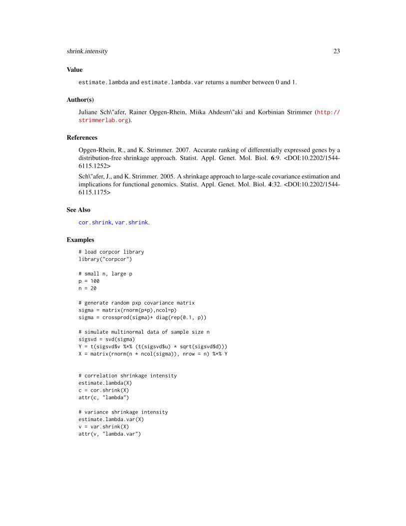
# load corpcor librarylibrary("corpcor")
# small n, large pp = 100n = 20
# generate random pxp covariance matrixsigma = matrix(rnorm(p*p),ncol=p)sigma = crossprod(sigma)+ diag(rep(0.1, p))
# simulate multinormal data of sample size nsigsvd = svd(sigma)Y = t(sigsvd$v %*% (t(sigsvd$u) * sqrt(sigsvd$d)))X = matrix(rnorm(n * ncol(sigma)), nrow = n) %*% Y
# correlation shrinkage intensityestimate.lambda(X)c = cor.shrink(X)attr(c, "lambda")
# variance shrinkage intensityestimate.lambda.var(X)v = var.shrink(X)attr(v, "lambda.var")
24 smtools
smtools Some Tools for Handling Symmetric Matrices
Description
sm2vec takes a symmetric matrix and puts the lower triagonal entries into a vector (cf. lower.tri).
sm.index lists the corresponding x-y-indices for each entry in the vector produced by sm2vec.
vec2sm reverses the operation by sm2vec and converts the vector back to a symmetric matrix. Ifdiag=FALSE the diagonal of the resulting matrix will consist of NAs. If order is supplied then theinput vector vec will first be rearranged accordingly.
Usage
sm2vec(m, diag = FALSE)sm.index(m, diag = FALSE)vec2sm(vec, diag = FALSE, order = NULL)
Arguments
m symmetric matrix
diag logical. Should the diagonal be included in the conversion to and from a vector?
vec vector of unique elements from a symmetric matrix
order order of the entries in vec
Value
A vector (sm2vec), a two-column matrix with indices (sm.index), or a symmetric matrix (vec2sm).
Author(s)
Korbinian Strimmer (http://strimmerlab.org/).
See Also
lower.tri.
Examples
# load corpcor librarylibrary("corpcor")
# a symmetric matrixm = rbind(c(3,1,1,0),c(1,3,0,1),c(1,0,2,0),c(0,1,0,2)

wt.scale 25
)m
# convert into vector (including the diagonals)v = sm2vec(m, diag=TRUE)v.idx = sm.index(m, diag=TRUE)vv.idx
# put back to symmetric matrixvec2sm(v, diag=TRUE)
# convert from vector with specified order of the elementssv = sort(v)svov = order(v)ovvec2sm(sv, diag=TRUE, order=ov)
wt.scale Weighted Expectations and Variances
Description
wt.var estimate the unbiased variance taking into account data weights.
wt.moments produces the weighted mean and weighted variance for each column of a matrix.
wt.scale centers and standardized a matrix using the weighted means and variances.
Usage
wt.var(xvec, w)wt.moments(x, w)wt.scale(x, w, center=TRUE, scale=TRUE)
Arguments
xvec a vector
x a matrix
w data weights
center logical value
scale logical value
Value
A rescaled matrix (wt.scale), a list containing the column means and variances (wt.moments), orsingle number (wt.var)

26 wt.scale
Author(s)
Korbinian Strimmer (http://strimmerlab.org).
See Also
weighted.mean, cov.wt.
Examples
# load corpcor librarylibrary("corpcor")
# generate some datap = 5n = 5X = matrix(rnorm(n*p), nrow = n, ncol = p)w = c(1,1,1,3,3)/9
# standardize matrixscale(X)wt.scale(X)wt.scale(X, w) # take into account data weights
Index
∗Topic algebrafast.svd, 7mpower, 11pseudoinverse, 17rank.condition, 19
∗Topic multivariatecor2pcor, 3corpcor-package, 2cov.shrink, 4invcov.shrink, 9pcor.shrink, 12powcor.shrink, 14rebuild.cov, 20shrink.intensity, 22wt.scale, 25
∗Topic utilitiessmtools, 24
attr, 13
cor, 5, 21cor.shrink, 9–12, 14, 15, 22, 23cor.shrink (cov.shrink), 4cor2pcor, 3, 6, 10, 13corpcor-package, 2cov, 5, 21cov.shrink, 2, 3, 4, 9, 10, 13cov.wt, 26crossprod.powcor.shrink
(powcor.shrink), 14
decompose.cov (rebuild.cov), 20decompose.invcov, 4decompose.invcov (rebuild.cov), 20
eigen, 11estimate.lambda, 5estimate.lambda (shrink.intensity), 22estimate.lambda.var, 5
fast.svd, 2, 7, 17, 18
invcor.shrink, 5, 15invcor.shrink (invcov.shrink), 9invcov.shrink, 2, 5, 6, 9, 13is.positive.definite (rank.condition),
19
lower.tri, 24
make.positive.definite(rank.condition), 19
mpower, 11, 15
pcor.shrink, 2, 4–6, 10, 12, 21pcor2cor (cor2pcor), 3powcor.shrink, 2, 10, 11, 14pseudoinverse, 3, 4, 17, 20pvar.shrink, 5pvar.shrink (pcor.shrink), 12
rank.condition, 19rebuild.cov, 20rebuild.invcov (rebuild.cov), 20
shrink.intensity, 22sm.index (smtools), 24sm2vec (smtools), 24smtools, 24solve, 8, 18svd, 7, 8, 19, 20
var, 5var.shrink, 9, 22, 23var.shrink (cov.shrink), 4vec2sm (smtools), 24
weighted.mean, 26wt.moments (wt.scale), 25wt.scale, 25wt.var (wt.scale), 25
27