
P olya urn models - Paris 13...
23
CIMPA Summer School 2014 Random structures, analytic and probabilistic approaches Nicolas Pouyanne P´olya urn models — Lecture notes — Contents 1 P´ olya urn: first steps 1 2 The approach in analytic combinatorics 3 3 The probabilistic approach 8 3.1 Introduction: an experimental computational approach .................. 9 3.1.1 Distributions ..................................... 9 3.1.2 Simulations of trajectories .............................. 9 3.1.3 Three urns ...................................... 10 3.2 Asymptotics of the composition vector, phase transition, figures ............. 12 3.3 Hint of proof ......................................... 19 1 P´olya urn: first steps Let R be a 2-dimensional square matrix having integral entries and U 0 a nonzero 2-dimensional (column) vector with nonnegative integral entries: R = a b c d , U 0 = α β . The P´olya urn process (U n ) n∈N with replacement matrix R and initial composition vector U 0 is in an imaging way defined as follows. An urn contains red and black balls. At time 0, it contains α red balls and β black ones. A ball is drawn uniformly at random from the urn and its colour is checked. If the drawn ball is red, it is replaced into the urn together with a red balls and b black ones; if the drawn ball is black, it is replaced into the urn as well, together with c red balls and d black ones. One get in this way a new composition vector U 1 . The random process (U n ) n∈N is recursively defined by iterating this mechanism. In this lecture, the following assumptions on R and U 0 are made: (i) R est balanced, i.e. a + b = c + d ≥ 1; (ii) R is “tenable”, i.e. b, c ≥ 0 and a ≤-1= ⇒ a|c and a|α and d ≤-1= ⇒ d|b and d|β . N. Pouyanne, P´olyaurns, CIMPA Summer School 2014 1
Transcript of P olya urn models - Paris 13...

CIMPA Summer School 2014Random structures, analytic and probabilistic approachesNicolas Pouyanne
Polya urn models— Lecture notes —
Contents
1 Polya urn: first steps 1
2 The approach in analytic combinatorics 3
3 The probabilistic approach 83.1 Introduction: an experimental computational approach . . . . . . . . . . . . . . . . . . 9
3.1.1 Distributions . . . . . . . . . . . . . . . . . . . . . . . . . . . . . . . . . . . . . 93.1.2 Simulations of trajectories . . . . . . . . . . . . . . . . . . . . . . . . . . . . . . 93.1.3 Three urns . . . . . . . . . . . . . . . . . . . . . . . . . . . . . . . . . . . . . . 10
3.2 Asymptotics of the composition vector, phase transition, figures . . . . . . . . . . . . . 123.3 Hint of proof . . . . . . . . . . . . . . . . . . . . . . . . . . . . . . . . . . . . . . . . . 19
1 Polya urn: first steps
Let R be a 2-dimensional square matrix having integral entries and U0 a nonzero 2-dimensional(column) vector with nonnegative integral entries:
R =
(a bc d
), U0 =
(αβ
).
The Polya urn process (Un)n∈N with replacement matrix R and initial composition vector U0 is in animaging way defined as follows. An urn contains red and black balls. At time 0, it contains α redballs and β black ones. A ball is drawn uniformly at random from the urn and its colour is checked.If the drawn ball is red, it is replaced into the urn together with a red balls and b black ones; if thedrawn ball is black, it is replaced into the urn as well, together with c red balls and d black ones. Oneget in this way a new composition vector U1. The random process (Un)n∈N is recursively defined byiterating this mechanism.
In this lecture, the following assumptions on R and U0 are made:(i) R est balanced, i.e. a+ b = c+ d ≥ 1 ;
(ii) R is “tenable”, i.e.(b, c ≥ 0
)and
(a ≤ −1 =⇒ a|c and a|α
)and
(d ≤ −1 =⇒ d|b and d|β
).
N. Pouyanne, Polya urns, CIMPA Summer School 2014 1

The balance hypothesis guarantees that the same number of balls S = a+ b = c+ d ≥ 1 is added atany step of time. Thanks to the tenability assumption, the process can never extinguish, which meansthat if a or d is negative, one can always respectively subtract −a or −d balls from the urn.
• In more rigorous terms,
(Un)n∈N =
(U
(1)n
U(2)n
)n∈N
is the N2 \ {0}-valued discrete time Markov chain defined by the transition conditional probabilitiesP
(Un+1 = Un +
(ab
) ∣∣∣Un) =U
(1)n
U(1)n + U
(2)n
;
P
(Un+1 = Un +
(cd
) ∣∣∣Un) =U
(2)n
U(1)n + U
(2)n
.
(1)
The balance assumption implies that U(1)n +U
(2)n = α+β+nS for any n: at any time n, the composition
of the urn is random but the total number of balls is deterministic.
• A complete definition of the Polya urn process as a Markov chain is given by the familyµxy
xy
∈N2\{0}
of probability measures on N2 \ {0} defined by:
∀(xy
)∈ N2 \ {0}, µx
y
=x
x+ yδxy
+
ab
+y
x+ yδxy
+
cd
,
where δP denotes the Dirac measure at P . Notice that the tenability assumption guarantees that(xy
)+
(ab
)and
(xy
)+
(cd
)belong to N2 \ {0} as soon as
(xy
)does.
[Generalisation to any finite number of colour, to random replacement matrices. In the present lecture,we will restrict ourselves to non random replacement matrices.]
Notations (spectral decomposition of R)Thanks to the balance assumption, S is an eigenvalue of tR. By elementary considerations a laPerron-Frobenius, the second eigenvalue m := a−c = d−b of tR is less than or equal to S. We denote
σ = m/S ≤ 1.
N. Pouyanne, Polya urns, CIMPA Summer School 2014 2

When (b, c) 6= (0, 0), let
v1 =S
b+ c
(cb
)and v2 =
S
b+ c
(1−1
).
The vectors v1 and v2 are eigenvectors of tR, respectively associated with the eigenvalues S and m.The dual basis (u1, u2) of linear eigenforms is given by the formulae
u1(x, y) =1
S(x+ y) and u2(x, y) =
1
S(bx− cy).
These vectors and linear forms will be useful later on in the lecture.
Note that in dimension larger than 3, the matrix R is not necessarily diagonalizable, even on C. Thisfact leads to some intricacy in the statement of the results but in a first approach, one can assumethat R is diagonalizable.
[Comment: urn models are useful in analysis of algorithms.]
2 The approach in analytic combinatorics
The approach by analytic combinatorics is due to Philippe Flajolet and his co-authors Philippe Dumas,Joaquim Gabarro, Helmut Pekari and Vincent Puyhaubert Puyhaubert in the 2000’s. There are twofounding articles, namely [4] et [3].
The very first idea consists in coding the urn composition by a sequence (Wn)n∈N of finite wordswritten in the 2-letter alphabet {r, b} (r for red, b for black). The initial composition is coded by
W0 = rr . . . rbb . . . b = rαbβ.
Drawing a ball in the urn amounts to choosing a letter in the word uniformly at random. When thechosen letter is an r, it is replaced in the world by the subword ra+1bb; when the chosen letter is a b,it is replaced by rcbd+1. Thus, the successive drawings give rise to a sequence of random words
W0,W1,W2 . . .
Of course, at any time n, the composition vector Un can be recovered by counting the number of r’sand the number of b’s in the word Wn.
Definition 1 (Histories of the process)
When n is a natural number, when
(u0
v0
),
(uv
)∈ N2 \ {0}, a history of length n leading from
(u0
v0
)to
(uv
)is a sequence of words W0 = ru0bv0 ,W1,W2, . . . ,Wn produced in that way, for which Wn
contains exactly u letters r et v letters b.
Of course, with this coding, because of the balance hypothesis, the wordWn always contains u0+v0+nSletters, whatever its history is. The key object of Flajolet’s method is the number of these histories:denote by
N. Pouyanne, Polya urns, CIMPA Summer School 2014 3

Hn
(u0 uv0 v
)
the number of histories of length n leading from
(u0
v0
)to
(uv
).
Exercise 1. When R =
(0 32 1
), code and count all histories of length 2 leading from
(20
)to
(44
).
[ One possible solution: start from W0 = r2. One can draw a tree of all possibilities: W1 ∈ {rb3r, r2b3},then W2 ∈ {rn6r, r3n4r, rnr2n3r, rn2r2n2r, rn3rn3} ou W2 ∈ {rb3rb3, r2b6, r4b4, r2br2b3, r2b2r2b2}. Amongst
the ten histories of length 2, six of them lead to
(44
)and four lead to
(26
): starting from two red balls, the
probability that the urn contains four red balls and four black ones after two drawings is 3/5.
Beware: in the example, the configuration rn3rn3 is reached by two different histories. We count histories, not
the different word that are potentially obtained. ]
Exercise 2 (this urn is Polya’s original one in his article published in 1930). Whenever R = SI2,compute all numbers Hn, n ≥ 0.[ This is elementary enumerative combinatorics. Make the picture of a path in N2 and count the histories thatfollow each of these paths. For any (p, q) ∈ N2 such that p+ q = n, one gets
Hn
(α α+ pSβ β + qS
)=
(np
)α(α+ S
). . .(α+ (p− 1)S
)β(β + S
). . .(β + (q − 1)S
)= n!Sn
(αS + p− 1
p
)(βS + q − 1
q
);
all others Hn vanish. ]
Exercise 3. For any urn, if N = α+ β, show that the total number of histories of length n starting
from
(αβ
)equals N
(N + S
)(N + 2S
). . .(N + (n− 1)S
)= n!Sn
(NS + n− 1
n
).
Generating series (or functions) are central tools in analytic combinatorics. Is the case of 2-coloururns, the relevant one is the trivariate generating series of histories: the variable x counts the finalnumber of red balls, the variable y counts the final number of black ones while the variable z countsthe lenth of the history. Thus, the replacement matrix R being given, denote
H
(x, y, z
∣∣∣∣ u0
v0
)=
∑u,v,n∈N
Hn
(u0 uv0 v
)xuyv
zn
n!.
Exercise 4. For any urn (i.e. for any R), H
(1, 1, z
∣∣∣∣ u0
v0
)=
(1
1− Sz
)u0+v0S
.
Exercise 5. For the original urn (R = SI2),
H
(x, y, z
∣∣∣∣ u0
v0
)=
xu0yv0
(1− SzxS)u0S (1− SzyS)
v0S
.
N. Pouyanne, Polya urns, CIMPA Summer School 2014 4

[ Computations on multivariate power series, based on the formula 1(1−X)N
=∑n≥0
(N + n− 1
n
)Xn. ]
[ Commentary on papers by P. Flajolet et al.: pointing an object amounts to make a partial derivativeon the generating series; proceeding to a replacement amounts to multiply the series by some appro-priate monomial. Such considerations lead to the following “Basic isomorphism”, stated and provenin [3]. ]
Theorem 1 (Flajolet, Dumas, Puyhaubert, 2006)Let x, y, z be complex numberes such that xy 6= 0. Let X(t) and Y (t) be the solutions of the CauchyProblem (formal version or analytic version)
dX
dt= Xa+1Y b
dY
dt= XcY d+1
X(0) = x, Y (0) = y.
(2)
Then, for any initial composition (u0, v0), for any z in some small enough neighbour of the origin(analytic version),
H
(x, y, z
∣∣∣∣ u0
v0
)= X(z)u0Y (z)v0 .
Example 1. Back to the original Polya urn for which R = SI2: the differential system writes X ′ =XS+1, Y ′ = Y S+1and can be solved. The solution of the Cauchy Problem is X(t) = x(1− StxS)−1/S ,Y (t) = y(1− StyS)−1/S . Theorem 1 provides a second proof of exercice 5.
Proof of Theorem 1. Consider the following differential operator on 2-variable functions:
D = xa+1yb∂
∂x+ xcyd+1 ∂
∂y.
The action of D on monomials is related to urn histories via the formula
D (xu0yv0) = u0xa+u0yb+v0 + v0x
c+u0yd+v0
= H1
(u0 u0 + av0 v0 + b
)xa+u0yb+v0 +H1
(u0 u0 + cv0 v0 + d
)xc+u0yd+v0
=∑u,v≥0
H1
(u0 uv0 v
)xuyv
which implies by induction that for any n ∈ N,
Dn (xu0yv0) =∑u,v≥0
Hn
(u0 uv0 v
)xuyv. (3)
N. Pouyanne, Polya urns, CIMPA Summer School 2014 5

[Notice that the Markov property of the urn process is expressed in this induction.] Besides, if (X,Y )is a solution of the differential system X ′ = Xa+1Y b, Y ′ = XcY d+1, then
d
dt(X(t)u0Y (t)v0) = u0X(t)a+u0Y (t)b+v0 + v0X(t)c+u0Y (t)d+v0
= D (xu0yv0)∣∣∣∣ x = X(t)y = Y (t)
which extends to an analogous formula for the n-th derivative. Gathering these results leads succes-sively to
H
(X(t), Y (t), z
∣∣∣∣ u0
v0
)=∑n≥0
Dn (xu0yv0)∣∣∣∣ x = X(t)y = Y (t)
zn
n!
=∑n≥0
dn
dtn(X(t)u0Y (t)v0)
zn
n!.
Thanks to Taylor Formula (analytic or formal version) one concludes by
H
(X(t), Y (t), z
∣∣∣∣ u0
v0
)= X(t+ z)u0Y (t+ z)v0 .
The final result follows taking the value at the origin (t = 0).
When the differential system can be solved, applying Theorem 1 leads to a close form of the Hfunction. When this is possible, on gets very accurate probabilistic consequences on the distributionof the composition of the urn at finite time, or on the asymptotics of the process as well. We givehereunder a couple of examples, essentially drawn from [4] and [3].
Remark. 1- One gets immediately from Theorem 1 that
H
(x, y, z
∣∣∣∣ u0
v0
)= H
(x, y, z
∣∣∣∣ 10
)u0H
(x, y, z
∣∣∣∣ 01
)v0.
This formula evokes some (combinatoric) convolution property. It has to be related to the branchingproperty of the continuous time corresponding urn process, that leads to a similar equation on theFourier transforms of large urns limit laws. See [2]. A direct link between both properties remainsan open question.
Example 2. Take the urn having
(0 11 0
)as replacement matrix.. [ Friedmann’s urn. Talk about
the propaganda campaign used by P. Flajolet. ] The Cauchy Problem writesX ′ = XYY ′ = XYX(0) = x, Y (0) = y
and can be easily solved. One finds
H
(x, y, z
∣∣∣∣ u0
v0
)=
(x(x− y)
x− yez(x−y)
)u0 ( y(y − x)
y − xez(y−x)
)v0.
N. Pouyanne, Polya urns, CIMPA Summer School 2014 6

For example, when one starts with a sole red ball, the probability generating function of the numberof red balls is
E(xU
(1)n
)=
[zn
n!
]∑n,k
P(U (1)n = k)xk
zn
n!= [zn]H
(x, 1, z
∣∣∣∣ 10
),
since the total number of histories of length n starting from one red ball is n! (see Exercise 3). Usingthe explicit expression of H, one gets
E(xU
(1)n
)= [zn]
x(x− 1)
x− ez(x−1).
This function of the z-variable has a simple pole at z = log xx−1 as unique singularity. Since this function
of the x-variable is analytic at 1, singularity analysis shows that one can apply Hwang’s Quasi-power
Theorem: the mean and the variance of U(1)n are both asymptotically proportional to n, and the
number of red balls at time n (i.e. the random variable U(1)n ) satisfies a Law of Large Numbers and a
Central Limit Theorem as well (Gaussian distribution).
Exemple 3. This example is the central one in [4]. It deals with the urn process that models the leaves
of a 2− 3-tree, which is an important search tree algorithm. Its replacement matrix is
(−2 34 −3
).
Here, the Cauchy Problem writes X ′ = X−1Y 3
Y ′ = X4Y −2
X(0) = x, Y (0) = y.(4)
Pose Z = X2; one gets successively Z ′ = 2Y 3 and Z ′′ = 6Z2. Multiply first by Z ′ then integrate. Thisleads to whow that Z is necessarily a solution of the Cauchy Problem
Z ′2 = 4Z3 − g3
Z(0) = x2
Z ′(0) = 2y3(5)
where g3 = 4(x6 − y6). This equation is solved using the famous and beautiful theory of ellipticfunctions. Quickly said, let ℘(z) = ℘(z; 0,−4) be the elliptic Weiestrass function, associated to the(so-called) invariantss g2 = 0 et g3 = −4: if one denotes
ω =1
2B
(1
6,1
3
)(Euler Beta function) and if Λ denotes the hexagonal lattice
Λ = ω(eiπ/6Z + e−iπ/6Z
),
then ℘ is the meromorphic function of the complex plane defined on the complementary of the latticeΛ by
℘(z) =1
z2+
∑λ∈Λ\(0)
[1
(z + λ)2 −1
λ2
].
N. Pouyanne, Polya urns, CIMPA Summer School 2014 7
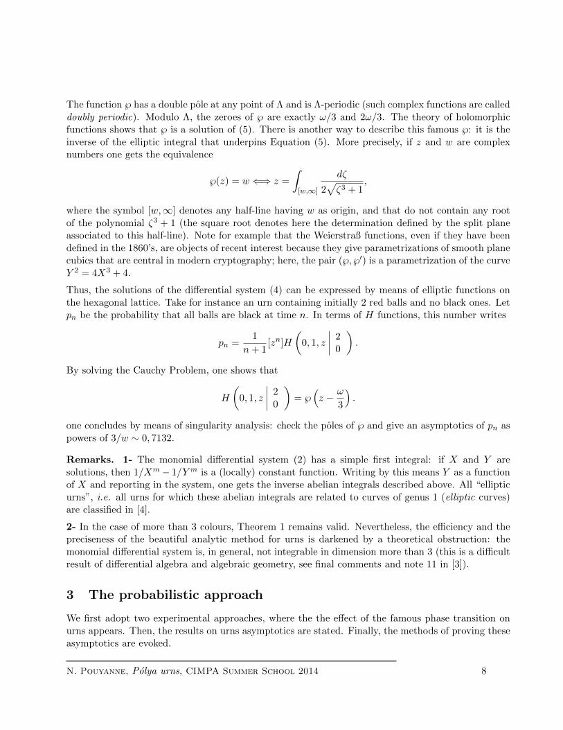
The function ℘ has a double pole at any point of Λ and is Λ-periodic (such complex functions are calleddoubly periodic). Modulo Λ, the zeroes of ℘ are exactly ω/3 and 2ω/3. The theory of holomorphicfunctions shows that ℘ is a solution of (5). There is another way to describe this famous ℘: it is theinverse of the elliptic integral that underpins Equation (5). More precisely, if z and w are complexnumbers one gets the equivalence
℘(z) = w ⇐⇒ z =
∫[w,∞]
dζ
2√ζ3 + 1
,
where the symbol [w,∞] denotes any half-line having w as origin, and that do not contain any rootof the polynomial ζ3 + 1 (the square root denotes here the determination defined by the split planeassociated to this half-line). Note for example that the Weierstraß functions, even if they have beendefined in the 1860’s, are objects of recent interest because they give parametrizations of smooth planecubics that are central in modern cryptography; here, the pair (℘, ℘′) is a parametrization of the curveY 2 = 4X3 + 4.
Thus, the solutions of the differential system (4) can be expressed by means of elliptic functions onthe hexagonal lattice. Take for instance an urn containing initially 2 red balls and no black ones. Letpn be the probability that all balls are black at time n. In terms of H functions, this number writes
pn =1
n+ 1[zn]H
(0, 1, z
∣∣∣∣ 20
).
By solving the Cauchy Problem, one shows that
H
(0, 1, z
∣∣∣∣ 20
)= ℘
(z − ω
3
).
one concludes by means of singularity analysis: check the poles of ℘ and give an asymptotics of pn aspowers of 3/w ∼ 0, 7132.
Remarks. 1- The monomial differential system (2) has a simple first integral: if X and Y aresolutions, then 1/Xm− 1/Y m is a (locally) constant function. Writing by this means Y as a functionof X and reporting in the system, one gets the inverse abelian integrals described above. All “ellipticurns”, i.e. all urns for which these abelian integrals are related to curves of genus 1 (elliptic curves)are classified in [4].
2- In the case of more than 3 colours, Theorem 1 remains valid. Nevertheless, the efficiency and thepreciseness of the beautiful analytic method for urns is darkened by a theoretical obstruction: themonomial differential system is, in general, not integrable in dimension more than 3 (this is a difficultresult of differential algebra and algebraic geometry, see final comments and note 11 in [3]).
3 The probabilistic approach
We first adopt two experimental approaches, where the the effect of the famous phase transition onurns appears. Then, the results on urns asymptotics are stated. Finally, the methods of proving theseasymptotics are evoked.
N. Pouyanne, Polya urns, CIMPA Summer School 2014 8

3.1 Introduction: an experimental computational approach
3.1.1 Distributions
As a first approach, for any urn, consider the probability generating function of the number of (say)
red balls at time n, starting from the initial composition
(u0
v0
):
pn
(x
∣∣∣∣ u0
v0
):=∑u≥0
P(u0,v0)
(U (1)n = u
)xu = E(u0,v0)
(xU
(1)n
).
Since the total number af balls at time n is deterministic, this probability generating function describesthe whole distribution of the urn composition at time n. This probability generating function can beexpressed by means of H functions: denote by
Hn
(x, y
∣∣∣∣ u0
v0
):=
∑u,v≥0
Hn
(u0 uv0 v
)xuyv = n! [zn]H
(x, y, z
∣∣∣∣ u0
v0
)
the generating series (it is a 2-variable polynomial) of histories of length n starting from
(u0
v0
). Then,
Hn
(1, 1
∣∣∣∣ u0
v0
)is the total number of histories of length n starting from
(u0
v0
)(see Exercise 3) and
pn
(x
∣∣∣∣ u0
v0
)=
Hn
(x, 1
∣∣∣∣ u0
v0
)Hn
(1, 1
∣∣∣∣ u0
v0
) .
Thus, it suffices to compute Hn
(x, y
∣∣∣∣ u0
v0
), or even Hn
(x, 1
∣∣∣∣ u0
v0
)to get pn. But, as shown in the
proof of Theorem 1, the bivariate function Hn
(x, y
∣∣∣∣ u0
v0
)satisfies Equation (3), namely
Hn
(x, y
∣∣∣∣ u0
v0
)= Dn (xu0yv0) .
As a matter of consequence, by means of computer algebra, starting from the monomial xu0yv0 , itsuffices to make an iteration of the operator D to get a symbolic expression of the entire function
Hn
(x, y
∣∣∣∣ u0
v0
). The probability generating function pn is then extracted by substitutions (y = 1
and x = 1). By this means, the distribution of red balls at given times can be graphically represented.This is done below for three particular urns and initial compositions.
3.1.2 Simulations of trajectories
Another approach consists in simulating the random successive compositions of an urn. One can by thismeans have a representation of trajectories of the composition vector, namely {(n,Un) , n = 0, 1, 2 . . . }
N. Pouyanne, Polya urns, CIMPA Summer School 2014 9

for different random drawings. Taking only the first coordinate of Un leads to trajectories of the numberof red balls, namely {(
n,U (1)n
), n = 0, 1, 2 . . .
}.
This is done below for three particular urns and initial compositions.
3.1.3 Three urns
Consider the urn processes having respectively
I2 =
(1 00 1
), R1 =
(1 1211 2
)and R2 =
(12 12 11
)
as matrix transitions. The drawings presented hereunder are made taking respectively
(25
),
(10
)and
(10
)as initial composition. All graphics are different representations of the number of red balls
contained in the urn.
1- Very first histograms
Any picture is made for a given number n of drawings in the urn. On the x-axis, the number of redballs in the urn after n drawings. On the y-axis, the number of histories of length n starting from theinitial composition. Points at integer abscissae are related by line segments.
n = 1 n = 2 n = 3 n = 10
Red balls in the original Polya urn I2 after n drawings, initial composition (2, 5)
N. Pouyanne, Polya urns, CIMPA Summer School 2014 10

n = 1 n = 2 n = 3 n = 10
Red balls in the urn R1 after n drawings, initial composition (1, 0)
n = 1 n = 2 n = 3 n = 10
Red balls in the urn R2 after n drawings, initial composition (1, 0)
[ Comments. ]
2- Very first trajectories
For a given urn, we draw three different trajectories, corresponding to three random sequences ofdrawings in the urn. On the x-axis, the number of drawings (discrete time); the maximal number ofdrawings is successively N = 100, 1000, 50000. On the y-axis, the number of red balls in the urn.
N = 100 N = 1000 N = 50000
Red balls in three sequences of N drawings in an original Polya urn I2, initial composition (2, 5)
N. Pouyanne, Polya urns, CIMPA Summer School 2014 11

N = 100 N = 1000 N = 50000
Red balls in three sequences of N drawings in an urn R1, initial composition (1, 0)
N = 100 N = 1000 N = 50000
Red balls in three sequences of N drawings in an urn R2, initial composition (1, 0)
[ Comments. ]
3.2 Asymptotics of the composition vector, phase transition, figures
The composition vector Un of a Polya urn process has different asymptotics regimes when n tendsto infinity, depending on the spectral decomposition of the replacement matrix R. In this section,we state, comment and illustrate these asymptotic results. All of them can be extended in higherdimension (any finite number of colours). Methods of proofs are introduced in Section 3.3.
Take a two-colour Polya urn with replacement matrix R =
(a bc d
)and initial composition vector
U0 =
(αβ
). We adopt the notations of Section 1, especially the balance S = a+ b = c+ d, the second
eigenvalue m = a− c = d− b, the tR-eigenvectors v1, v2 and, above all, the ratio
σ = m/S.
N. Pouyanne, Polya urns, CIMPA Summer School 2014 12
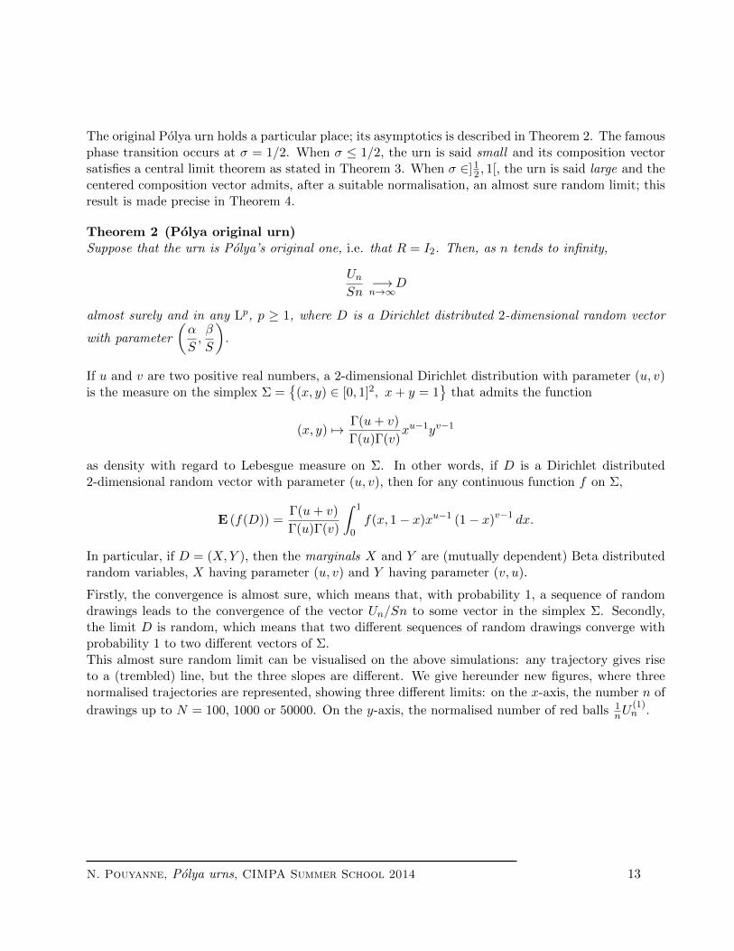
The original Polya urn holds a particular place; its asymptotics is described in Theorem 2. The famousphase transition occurs at σ = 1/2. When σ ≤ 1/2, the urn is said small and its composition vectorsatisfies a central limit theorem as stated in Theorem 3. When σ ∈]1
2 , 1[, the urn is said large and thecentered composition vector admits, after a suitable normalisation, an almost sure random limit; thisresult is made precise in Theorem 4.
Theorem 2 (Polya original urn)Suppose that the urn is Polya’s original one, i.e. that R = I2. Then, as n tends to infinity,
UnSn−→n→∞
D
almost surely and in any Lp, p ≥ 1, where D is a Dirichlet distributed 2-dimensional random vector
with parameter
(α
S,β
S
).
If u and v are two positive real numbers, a 2-dimensional Dirichlet distribution with parameter (u, v)is the measure on the simplex Σ =
{(x, y) ∈ [0, 1]2, x+ y = 1
}that admits the function
(x, y) 7→ Γ(u+ v)
Γ(u)Γ(v)xu−1yv−1
as density with regard to Lebesgue measure on Σ. In other words, if D is a Dirichlet distributed2-dimensional random vector with parameter (u, v), then for any continuous function f on Σ,
E (f(D)) =Γ(u+ v)
Γ(u)Γ(v)
∫ 1
0f(x, 1− x)xu−1 (1− x)v−1 dx.
In particular, if D = (X,Y ), then the marginals X and Y are (mutually dependent) Beta distributedrandom variables, X having parameter (u, v) and Y having parameter (v, u).
Firstly, the convergence is almost sure, which means that, with probability 1, a sequence of randomdrawings leads to the convergence of the vector Un/Sn to some vector in the simplex Σ. Secondly,the limit D is random, which means that two different sequences of random drawings converge withprobability 1 to two different vectors of Σ.This almost sure random limit can be visualised on the above simulations: any trajectory gives riseto a (trembled) line, but the three slopes are different. We give hereunder new figures, where threenormalised trajectories are represented, showing three different limits: on the x-axis, the number n of
drawings up to N = 100, 1000 or 50000. On the y-axis, the normalised number of red balls 1nU
(1)n .
N. Pouyanne, Polya urns, CIMPA Summer School 2014 13

N = 100 N = 1000 N = 500001nU
(1)n in three sequences of N drawings in an original Polya urn I2, initial composition (2, 5)
One can also visualise the Beta distributed limit of the normalised number of red balls. Hereunder,the figure on the left represent the (exact) distribution of the normalised number of red balls in the
urn after n = 200 drawings. On the x-axis, 1n
(U
(1)n −EU
(1)n
). On the y-axis, the probability; it has
been computed from the probability generating function pn introduced above. The figure on the rightrepresents the graph of the density of the centered Beta distribution with parameter (2, 5), namelythe function x 7→ 1
B(2,5) (x− µ)1 (1− x+ µ)4 where µ = B(3, 5)/B(2, 5) = 2/7 is the expectation.
n = 200
Normalised distribution of the number of red balls
in an original Polya urn I2, initial composition (2, 5)
Density of a centered
Beta (2, 5) distribution
Theorem 3 (Small urns)Suppose that the urn is small, which means that σ < 1/2. Then as n tends to infinity,
(i)Unn
converges to v1, almost surely and in any Lp, p ≥ 1;
(ii) assume further that R is not triangular, i.e. that bc 6= 0. Then,Un − nv1√
nconverges in distribution
N. Pouyanne, Polya urns, CIMPA Summer School 2014 14

to a centered gaussian vector with covariance matrix
1
1− 2σ
bcm2
(b+ c)2
(1 −1−1 1
).
[ When σ = 1/2, one says also that the urn is small. In this case, assertion (i) holds as well whereas, when R
is not triangular, assertion (ii) must be replaced by: Un−nv1√n logn
converges in distribution to a centered Gaussian
vector with covariance matrix 14bc
(1 −1−1 1
). ]
Here, the convergence of Un/n is almost sure again, but the limit is deterministic: with probability 1,a sequence of random drawings leads to the convergence of the vector Un/n, but the limit is nowalways the same one (namely, v1). This phenomenon can be visualised on the trajectories for theurn R1: the three asymptotic slopes are identical. When the normalised trajectories are drawn, onegets the following pictures. Here again, on the x-axis, the number n of drawings up to N = 100, 1000
or 50000; on the y-axis, the normalised number of red balls 1nU
(1)n .
N = 100 N = 1000 N = 50000
1nU
(1)n in three sequences of N drawings in a small urn R1, initial composition (1, 0)
The convergence in distribution stated in (ii) is of a radically different nature. It means that thedistribution at finite time n converges to some given distribution when n tends to infinity. The limitdistribution is here normal. As before, for the R1-urn, with the help of the probability generating
function, the (exact) distribution of the number 1√n
(U
(1)n −EU
(1)n
)is drawn on the leftside figure for
n = 600. On the right, the graph of the density of the centered normal distribution with variance1
1−2σbcm2
(b+c)2= 5200
529 .
N. Pouyanne, Polya urns, CIMPA Summer School 2014 15
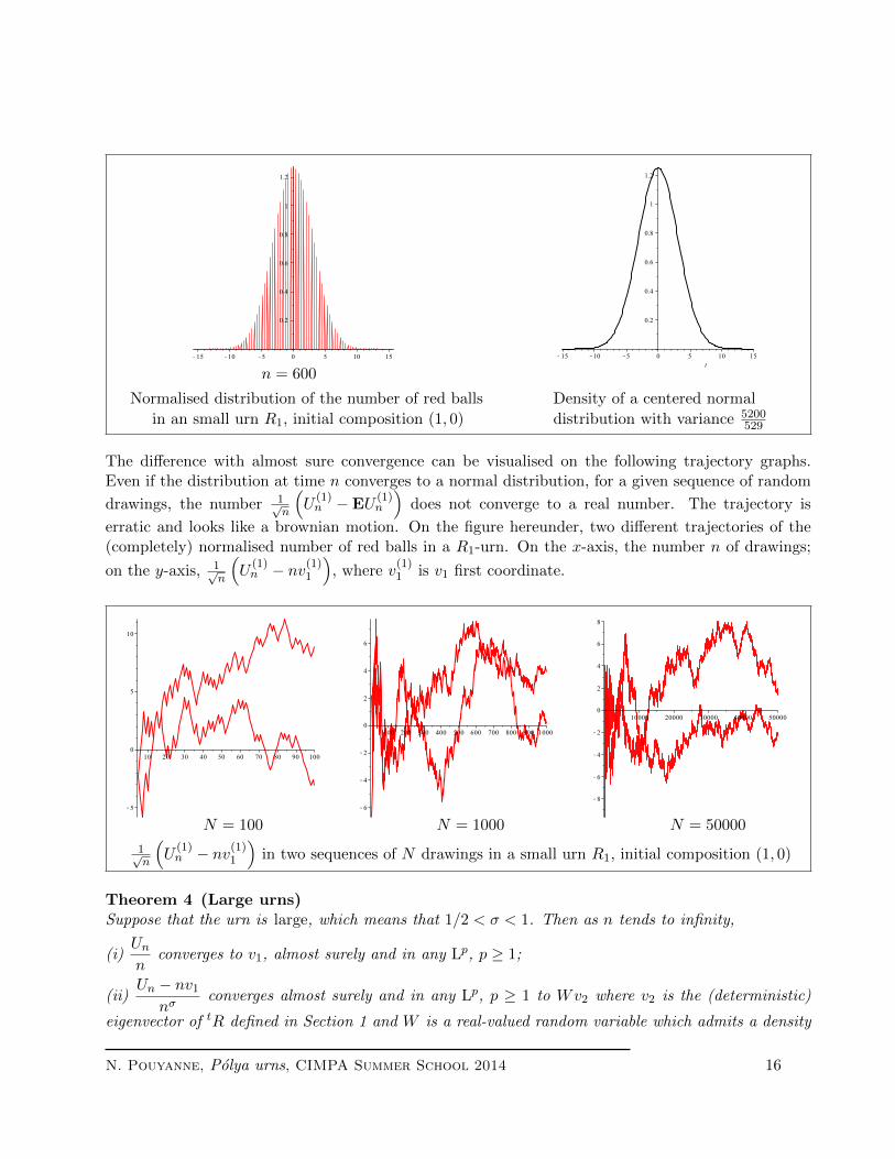
n = 600
Normalised distribution of the number of red balls
in an small urn R1, initial composition (1, 0)
Density of a centered normal
distribution with variance 5200529
The difference with almost sure convergence can be visualised on the following trajectory graphs.Even if the distribution at time n converges to a normal distribution, for a given sequence of random
drawings, the number 1√n
(U
(1)n −EU
(1)n
)does not converge to a real number. The trajectory is
erratic and looks like a brownian motion. On the figure hereunder, two different trajectories of the(completely) normalised number of red balls in a R1-urn. On the x-axis, the number n of drawings;
on the y-axis, 1√n
(U
(1)n − nv(1)
1
), where v
(1)1 is v1 first coordinate.
N = 100 N = 1000 N = 50000
1√n
(U
(1)n − nv(1)
1
)in two sequences of N drawings in a small urn R1, initial composition (1, 0)
Theorem 4 (Large urns)Suppose that the urn is large, which means that 1/2 < σ < 1. Then as n tends to infinity,
(i)Unn
converges to v1, almost surely and in any Lp, p ≥ 1;
(ii)Un − nv1
nσconverges almost surely and in any Lp, p ≥ 1 to Wv2 where v2 is the (deterministic)
eigenvector of tR defined in Section 1 and W is a real-valued random variable which admits a density
N. Pouyanne, Polya urns, CIMPA Summer School 2014 16

and is supported by the whole real line. Besides, with the notations of Section 1,
EW =Γ(α+βS
)Γ(α+βS + σ
) bα− cβS
.
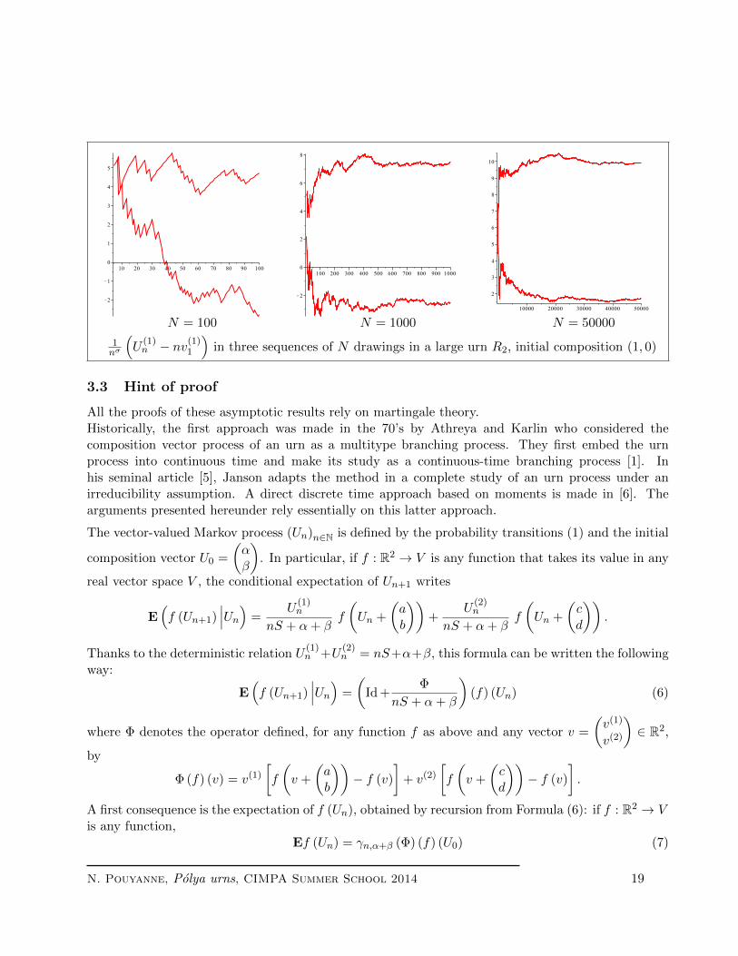
Assertion (i) is the same one as in the case of small urns. We make the same simulations as before forthe urn R2. The convergence to the (same) limit is visibly much slower, due to the second order termwhich grows like nσ with σ ' 0.77 (instead of
√n for small urns). This second order term was already
seeable on the trajectories of the number of red balls: the three slopes do not look not as similar as inthe case of the small urn R1 (but they really tend to a same one as N tends to infinity). Hereunder,again, on the x-axis, the number n of drawings up to N = 100, 1000 or 50000; on the y-axis, the
normalised number of red balls 1nU
(1)n .
N = 100 N = 1000 N = 50000
1nU
(1)n in three sequences of N drawings in a large urn R2, initial composition (1, 0)
Almost sure convergence implies convergence in distribution. In particular, by formal computationof the probability generating function of red balls, the shape of W ’s density can be approached asalready done (Beta function for the original Polya urn, Gauss function for a small urn). The Fouriertransform of W can be expressed in terms of the inverse of some suitable abelian integral (see [2]).Despite of this, very few is known about its density. The figure hereunder shows the graph of the
density of W −EW , approached by the (exact) distribution of 1nσ
(U
(1)n −EU
(1)n
)for n = 40, 120 and
800.
N. Pouyanne, Polya urns, CIMPA Summer School 2014 17

n = 40 n = 120 n = 800
Normalised distribution of the number of red balls
in a large urn R2 after n drawings, initial composition (1, 0)
A remarkable fact: the distribution W depends on the initial composition of the urn, which does nothappen for small urns. The graphs hereunder illustrate this property, representing W −EW ’s densityfor the large urn R2 starting with respectively (1, 0), (1, 1) and (2, 1) as initial composition vector.
(α, β) = (1, 0) (α, β) = (1, 1) (α, β) = (2, 1)
Normalised distribution of the number of red balls in a large urn R2
after 500 drawings, initial composition (α, β)
The last illustration concerns the second term order which has a random asymptotics. Two normalisedtrajectories of the number of red balls in an R2-urn up to time N = 100, 1000 and 50000 are plot-
ted. The convergence of 1nσ
(U
(1)n − nv(1)
1
)is here almost sure: for (almost) any sequence of random
drawings in the large urn, this random variable converges to a (random) limit. The situation is verydifferent from the small urn case, where a given trajectory do not give rise to the convergence of thesecond order normalised number of red balls. Here again, on the x-axis, the number n of drawings up
to N ; on the y-axis, the second order normalised number of red balls 1nσ
(U
(1)n − nv(1)
1
). Here again,
v(1)1 denotes v1 first coordinate
N. Pouyanne, Polya urns, CIMPA Summer School 2014 18
N = 100 N = 1000 N = 50000
1nσ
(U
(1)n − nv(1)
1
)in three sequences of N drawings in a large urn R2, initial composition (1, 0)
3.3 Hint of proof
All the proofs of these asymptotic results rely on martingale theory.Historically, the first approach was made in the 70’s by Athreya and Karlin who considered thecomposition vector process of an urn as a multitype branching process. They first embed the urnprocess into continuous time and make its study as a continuous-time branching process [1]. Inhis seminal article [5], Janson adapts the method in a complete study of an urn process under anirreducibility assumption. A direct discrete time approach based on moments is made in [6]. Thearguments presented hereunder rely essentially on this latter approach.
The vector-valued Markov process (Un)n∈N is defined by the probability transitions (1) and the initial
composition vector U0 =
(αβ
). In particular, if f : R2 → V is any function that takes its value in any
real vector space V , the conditional expectation of Un+1 writes
E(f (Un+1)
∣∣∣Un) =U
(1)n
nS + α+ βf
(Un +
(ab
))+
U(2)n
nS + α+ βf
(Un +
(cd
)).
Thanks to the deterministic relation U(1)n +U
(2)n = nS+α+β, this formula can be written the following
way:
E(f (Un+1)
∣∣∣Un) =
(Id +
Φ
nS + α+ β
)(f) (Un) (6)
where Φ denotes the operator defined, for any function f as above and any vector v =
(v(1)
v(2)
)∈ R2,
by
Φ (f) (v) = v(1)
[f
(v +
(ab
))− f (v)
]+ v(2)
[f
(v +
(cd
))− f (v)
].
A first consequence is the expectation of f (Un), obtained by recursion from Formula (6): if f : R2 → Vis any function,
Ef (Un) = γn,α+β (Φ) (f) (U0) (7)
N. Pouyanne, Polya urns, CIMPA Summer School 2014 19

where γn,τ is the real polynomial defined by
γn,τ (X) =
n−1∏k=0
(1 +
X
kS + τ
)(τ is a non zero real number; if n = 0, this empty product equals 1). Notice that, thanks to StirlingFormula, when z is any complex number, one gets the asymptotics
γn,τ (z) =Γ(τS
)Γ(τ+zS
)n zS
(1 +O
(1
n
))where Γ denotes Euler Gamma function. Formulae (6) and (7) are basic tools for the present proof.When f 6= 0 is an eigenvector of Φ related to the eigenvalue λ, i.e. when Φ (f) = λf , thenγn,τ (Φ) (f)(v) = γn,τ (λ)×f(v) so that Stirling Formula gives immediately the asymptotics of Ef (Un)when n tends to infinity. With this elementary remark, one can evaluate the asymptotic joint momentsof Un’s coordinates, leading to the proof of Theorem 4. Theorem 2 can also be proven with such tools.Classically, the proof of the small irreducible case (Theorem 3) is made by embedding the process intocontinuous time, and coming back to discrete time using some suitable ranom stopping-time. See [5]for a complete proof.
Exercise 6.6.1- (Linear functions)Show that if V is a real vector space and if f : R2 → V is linear, then
Φ(f) = f ◦A
where A : R2 → R2 is defined by A(v) = A
(v(1)
v(2)
):= tR
(v(1)
v(2)
)=
(a cb d
)(v(1)
v(2)
).
6.2- (Vector-valued martingale)
Denote τ := α + β. Show that the process(γn,τ
(tR)−1
(Un))n
is a martingale (with regard to the
natural filtration) as soon as it is defined, i.e. as soon as all matrices I2 + 1kS+τR, k ∈ N are invertible.
Show that this martingale is not defined if, and only if m ≤ −1 and S divides m+ α+ β.
[Apply 6.1- to f = Id. This leads to E(Un+1
∣∣Un) =(I2 + 1
nS+τA)
(Un). This implies all the answers, because
A is diagonalizable, with eigenvalues S and m.]
6.3- (Expectation)Let u1 and u2 be the eigenforms defined in Section 1. Verify (or remember!) that u1 ◦ A = Su1 andu2 ◦A = mu2. Show that for any n ∈ N,
Eu1 (Un) = n+τ
S
and, when n tends to infinity,
Eu2 (Un) =Γ(τS
)Γ(τS + σ
) bα− cβS
nσ(
1 +O
(1
n
)).
N. Pouyanne, Polya urns, CIMPA Summer School 2014 20

When R 6= SI2, using that v = u1(v)v1 + u2(v)v2 for any vector v ∈ R2, show that, when n tends toinfinity,
EUn ∼ nv1
[An induction using 6.1- leads to Eu1 (Un) = γn,τ (S)× u1 (U0) = nS+ττ × τ
S . For u2, apply Stirling Formula to
Eu2 (Un) = γn,τ (m) × u2 (U0) with a O-remainder. The third assertion is obtained by addition of asymptotic
developments.]
6.4- (Real-valued projected martingales)Show that (
u1 (Un)
nS + τ
)n
is an almost surely bounded (thus convergent) martingale and compute its expectation. Show that(u2 (Un)
γn,τ (m)
)n
is a martingale as well, as soon as m ≥ 0 or m+ τ is not a multiple of S.
[Using 6.1- again, one gets E(u1 (Un+1)
∣∣Un) =(
1 + SnS+τ
)× u1 (Un), so that E
(u1(Un+1)(n+1)S+τ
∣∣Un) = u1(Un)nS+τ ,
proving the martingale property. Same argument from E(u2 (Un+1)
∣∣Un) =(
1 + mnS+τ
)× u2 (Un). ]
6.5- (Second moments)Denote by P and Q the 2-variable polynomials defined by
P (x, y) = u1(x, y)
(u1(x, y) + 1
)and Q(x, y) =
(u1(x, y) + σ
)u2(x, y).
Show that Φ(P ) = 2SP and Φ(Q) = (S +m)Q and prove the asymptotics when n tends to infinity
EP (Un) = n2
(1 +O
(1
n
))and
EQ (Un) =Γ(τS
)Γ(τS + σ
) bα− cβS
n1+σ
(1 +O
(1
n
))(if one feels depressed, one can just show that Q (Un) ∈ O
(n1+σ
), :-)).
Suppose that σ 6= 1/2 and denote
R = u22 −
bcσ2
1− 2σu1 + (b− c)σu2.
Show that, in this case, Φ (R) = 2mR and that, when n tends to infinity,
ER (Un) =Γ(τS
)Γ(τS + 2σ
)R (α, β)n2σ
(1 +O
(1
n
)).
N. Pouyanne, Polya urns, CIMPA Summer School 2014 21

Show that (1, u1, u2, P,Q,R) is a basis of the vector space R2[x, y] of polynomials of degree less thanor equal to 2. Write x2, xy and y2 in this basis and compute the asymptotics of the co-moment matrixE[Un
tUn]
and of the covariance matrix E[(Un −EUn) t (Un −EUn)
](one has to discuss whether
σ < 1/2 or σ > 1/2).
Check what happens when σ = 1/2 and do the same job using T = u22 + 2b−m
2 u2 instead of R.
[One gets Φ(P ), Φ(Q) and Φ(R) by simple computation. Since Φ(P ) = 2SP , EP (Un) = γn,τ (2S)×P (U0) and
the required asymptotics for EP (Un) is obtained thanks to Stirling Formula. Idem for EQ (Un) and ER (Un).
The remainder of the exercise is completely left to the reader.]
6.6- (For large urns, the second projected martingale is square-bounded)Suppose that σ > 1/2. Expressing u2
2 as a function of R, u1 and u2, show that the martingale(u2(Un)γn,τ (m)
)n
is bounded in L2, thus convergent.
[u22 = R+ bcσ2
1−2σu1 − (b− c)σu2, so that Eu22 (Un) = c1n2σ (1 +O(1/n)) + c2n+ c3n
σ (1 +O(1/n)) where c1, c2and c3 are constants. Since σ > 1/2, the principal term is the one in n2σ, proving that the martingale is square
bounded (use Stirling formula again to get the asymptotics of γn,τ (m)2). ]
Exercise 7 (triangular urn).
Assume that b = 0, so that R =
(S 0
S −m m
). Assume also that the initial number of black balls is
non zero, i.e. that β 6= 0 (and check that β = 0 leads to a degenerate process). Let as above u1 andu2 be the linear forms
u1(x, y) =x+ y
Sand u2(x, y) =
y
S.
For any p ∈ N∗, let also Ap and Bp be the bivariate polynomials
Ap = u1 (u1 + 1) . . . (u1 + p− 1) =Γ (u1 + p)
Γ (u1)
and
Bp = u2
(u2 + σ
). . .
(u2 + (p− 1)σ
)=
Γ (u2 + pσ)
Γ (u2).
Show that Φ (Ap) = pSAp (as always, even if R is not triangular) and that Φ (Bp) = pmBp for anyp ≥ 1. Deduce from this that, when n tends to infinity,
EBp (Un) =Γ(τS
)Γ(τS + pσ
) Γ(βS + pσ
)Γ(βS
) npσ(
1 +O
(1
n
)).
• Assume that m ≥ 1.Using the inversion formula
up2 =
p∑k=1
(−σ)p−k{pk
}Bk,
N. Pouyanne, Polya urns, CIMPA Summer School 2014 22
show that, for any p ≥ 1,
limn→∞
E
(u2 (Un)
nσ
)p=
Γ(τS
)Γ(τS + pσ
) Γ(βS + pσ
)Γ(βS
) . (8)
so that the number of black balls U(2)n = Su2 (Un) converges in law to a random variable having the
right side of Equality (8) as p-th moment (to make a complete proof of that fact, one has to checkthat a distribution having such a p-th moment is determined by its moments, which can be done bycomputing the asymptotics of (8) as p tends to infinity with the help of Stirling Formula). This lawcan be related to stable laws or to Mittag-Leffler ones.
• Assume that m = 0. Show that the process is deterministic (degenerate case).
• Assume that m ≤ −1. Show that the number of black balls tends almost surely to zero (degeneratecase again).
References
[1] K.B. Athreya and S. Karlin. Embedding of urn schemes into continuous time Markov branchingprocesses and related limit theorems. Ann. Math. Statist, 39:1801–1817, 1968.
[2] B. Chauvin, N. Pouyanne, and R. Sahnoun. Limit distributions for large Polya urns. AnnalsApplied Prob., 21(1):1–32, 2011.
[3] Philippe Flajolet, Philippe Dumas, and Vincent Puyhaubert. Some exactly solvable models of urnprocess theory. In Philippe Chassaing, editor, Fourth Colloquium on Mathematics and ComputerScience, volume AG of DMTCS Proceedings, pages 59–118, 2006.
[4] Philippe Flajolet, Joaquim Gabarro, and Helmut Pekari. Analytic urns. Annals of Probability,33:1200–1233, 2005.
[5] S. Janson. Functional limit theorem for multitype branching processes and generalized Polya urns.Stochastic Processes and their Applications, 110:177–245, 2004.
[6] N. Pouyanne. An algebraic approach to polya processes. Annales de l’Institut Henri Poincare,44:293–323, 2008.
N. Pouyanne, Polya urns, CIMPA Summer School 2014 23


![P olya urn models - Paris 13 Universitynicodeme/nablus14/nafiles/... · 2014-08-13 · [Comment: urn models are useful in analysis of algorithms.] 2 The approach in analytic combinatorics](https://static.fdocuments.net/doc/165x107/5e97e620551df114ca77c888/p-olya-urn-models-paris-13-university-nicodemenablus14nafiles-2014-08-13.jpg)


