P and S velocity structure beneath the Toba caldera

complex (Northern Sumatra) from local earthquake

tomography

5

10

15

20

25

Ivan Koulakov (1, 2),

Tedi Yudistira (3),

Birger-G. Luehr (2),

and Wandono (4)

(1) Institute of Petroleum Geology and Geophysics, SB RAS,

Prospekt Akademika Koptuga, 3, Novosibirsk, 630090, Russia

e-mail: ivan2art@gmail.com

Phone: +7 383 3309201

(2) GeoForschungsZentrum Potsdam

Telegrafenberg, 14473, Potsdam, Germany

ase@gfz-potsdam.de (B.Luehr)

(3) Department of Geophysics Institut Teknologi Bandung,

tedi@geoph.itb.ac.id (Yudistira)

(4) Meteorological and Geophysical Agency (BMG), Jakarta

Jl. Angkasa I/2, Jakarta 10720,

wandono@bmg.go.id (Wandono)

to be submitted to Geophysical Journal International

Novosibirsk, April 2008

30

35

40

45

ABSTRACT In this paper, we investigate the crustal and uppermost mantle structure beneath Toba caldera,

which is known as the location of one of the largest Cenozoic eruptions on Earth. The most

recent event occurred 74,000 years BP, and had a significant global impact on climate and the

biosphere. In this study, we revise data on local seismicity in the Toba area recorded by a

temporary network in 1995. We applied the newest version of the LOTOS-07 algorithm, which

includes absolute source location, optimization of the starting 1D velocity model, and iterative

tomographic inversion for 3D seismic structure and source parameters. Special attention is paid

to verification of the obtained results. In particular, we constructed a synthetic model that

reproduces the same pattern as that obtained after inversion of the real data. This model was used

to estimate the real amplitudes of anomalies beneath Toba, which do not exceed 18%

perturbation. We compare our results for Toba with two other models beneath the volcanic arcs

of Central Andes and Central Java. We found some similar features and differences, but did not

observe any specific features in the seismic structure which could characterize Toba as a super

volcano.

2

1. Introduction The Toba volcanic complex, located in northern Sumatra, Indonesia, is part of a 5,000 km long

volcanic chain along the Sunda arc (Figure 1). Toba volcano produced the largest known

volcanic eruption on earth during the past 2 million years (Smith & Bailey, 1968). About 74,000

years BP, around 2,800 cubic kilometers of magma were erupted. The eruption led to the final

formation of one of the largest calderas, the 35x100 km wide Toba caldera. Super scale eruptions

at Toba have occurred several times (at least four eruptions of more than VEI 7 over the last 2

million years). In this sense, Toba seems to be a singularity in a chain of more than one hundred

other volcanoes with explosive potential along the Sunda arc. The reasons for this unique

behavior of the Toba volcanic activity are not yet clearly understood. We believe that

understanding the mechanisms of the origin of such supervolcanos will only be possible by

investigating the entire subduction complex beneath Toba and the surrounding areas. In addition,

comparison with subduction complexes from other areas can reveal specific features which

distinguish Toba from other volcanoes.

50

55

60

65

70

75

80

Another motivation for investigating the processes in the subduction complex of Sumatra is the

fact that subduction causes seismic activity. The Sumatra earthquake of 26.12.2004 and the

following aftershocks demonstrated the extremely damaging character of the collision processes

within the Sunda subduction zone.

Seismic tomography is a powerful tool for obtaining the 3D structure of P and S wave velocities

in the crust and the uppermost mantle. The obtained images provide key information about the

geodynamical processes at great depths. The distributions of earthquakes and the velocity

structure beneath Toba were previously studied in Fauzi et al. (1996) and Masturyono et al.

(2001). These studies were based on local seismicity data recorded by a temporarily passive

seismic experiment performed in 1995. Since then, no new seismic networks have been deployed

in this area. In this study, we revise the same data from the Toba area, using another tomographic

algorithm, LOTOS-07. This algorithm has some important features compared to the code used

for obtaining the previous results, such as quasi-continuous parameterization, 1D velocity

optimization, and a more effective algorithm for source location in a 3D model. It offers

effective and unbiased ways for verification of the obtained results based on synthetic modeling

and other tests. In this study, we pay special attention to studying the reliability of the results and

the quantitative evaluation of the derived parameters. In particular, in this study we use a new

technique for estimating the amplitudes of anomalies. Based on this technique, we show that in

3

the crust beneath Toba, the P velocity anomaly does not exceed 18%. This value is much lower

than that predicted by Masturyono et al. (2001).

An important purpose of this paper is to present two new features of the LOTOS-07 algorithms:

a 1D velocity optimization and a method for estimating the amplitudes of velocity anomalies. 85

90

95

100

105

110

2. Geological overview

The super large eruptions of Toba should be considered in the context of the entire subduction

complex beneath Sumatra. Sumatra Island is a northwest trending physiographic expression

located on the western edge of Sundaland, a southern extension of the Eurasian Continental Plate

(Figure 1 A, B). Sumatra Island has an area of about 435,000 km2, and a width of about 100-200

km in the northern part and about 350 km in the southern part. The main geographical trendlines

of the island are rather simple. Its backbone is formed by the Barisan Range, which runs along

the western side and constitutes the active volcanic arc and divides the west and the east coasts.

The distance between the Sunda trench and the Sumatran coast is about 200 km (Figure 1B). In

the offshore, a chain of islands forms the Forearc ridge, a local high between the trench and the

Sumatra coast. The island of Sumatra is interpreted to have been constructed by collision and

suturing of discrete micro continents in the late Pre-Tertiary times (Pulunggono and Cameron,

1984). At present, the Indian Ocean Plate is being subducted beneath the Eurasian Continental

Plate in a N20oE direction at a rate of about 5.5 cm/yr (Figure 1B). This zone is marked by the

active Sunda Arc-Trench system (Figure 1A) which extends for more than 5000 km, from Burma

in the north to where the Australian Plate is colliding with Eastern Indonesia in the south

(Hamilton, 1979). The input of sediments mainly comes from the Ganges River, India, leading to

the development of the largest accretionary wedge at a subduction zone on earth. The oblique

subduction of the Indian plate is responsible for strike-slip fault systems along Sumatra (e.g.,

Mentawai Fault System (MFS), Sumatra Fault System (SFS)).

In 1949, van Bemmelen (1949) reported that Lake Toba was surrounded by a vast layer of

ignimbrite rocks. Later researchers found rhyolite ash in Malaysia similar to the ignimbrites

around Toba, as well as 3000 km away in India (Aldiss & Ghazali, 1984), and on the seafloor of

the eastern Indian Ocean and the Bay of Bengal. These observations show that the Toba

eruption, dated at 74,000 years ago, was the most recent truly large eruption on Earth. All

information on the extent of the erupted Toba volcanic material has been compiled in Rose and

Chesner (1987), Chesner and Rose (1991), and Chesner et al. (1991). According to estimates in

4

these studies, the total amount of erupted material was about 2,800 km3. About 800 km3 was

ignimbrite that traveled swiftly over the ground away from the volcano, and the remaining 2,000

km

115

120

125

130

135

140

145

3 fell as ash, with the wind blowing most of it to the west. Such a huge eruption probably

lasted nearly two weeks. Ninkovich et al. (1978) estimated the height of the eruption column to

have been 50 to 80 km. Rose and Chesner (1987), after a study of the shapes of the ash shards,

concluded this estimate was too high by a factor of 5 or more. This event, called the Eruption of

the Youngest Toba Tuff (YTT), was responsible for the collapse structure of the Toba caldera

visible today (Van Bemmelen, 1949). It should be noted that besides the most recent large

eruption of 73,000 years ago, during the past 1·2 my, there have been at least three other ash

flow tuff eruptions from the caldera complex (Chesner and Rose, 1991; Chesner et al., 1991).

The older Toba units are the Middle Toba Tuff (MTT) (age 0.50 Ma, Chesner et al., 1991), the

Oldest Toba Tuff (OTT) (age 0.84 Ma, Diehl et al., 1987), and the Haranggoal Dacite Tuff

(HDT) (age 1.2 Ma, Nishimura et al., 1977). These were erupted alternately from northern and

southern vent areas in the present caldera (Chesner and Rose, 1991).

The eruption of such a huge amount of volcanic rock caused a large collapse, resulting in a huge

caldera. This caldera filled with water and created Lake Toba (Figure 1C). The Toba caldera, the

largest known Cenozoic caldera in the world, has a size of 30 by 100 km and a total relief of

1,700 m. After the YTT eruption, resurgent doming formed the massive Samosir Island and

Uluan Peninsula structural blocks. Lake sediments on Samosir indicate an uplift of at least 450

m. Additionally, post-YTT eruptions include a series of lava domes, the growth of the

solfatarically active Pusubukit volcano on the southwestern margin of the caldera, and the

formation of Sipisopiso volcano at the NW-most rim of the caldera. Lack of vegetation suggests

that this volcano may be only a few hundred years old. There have been no eruptions

documented for Toba in historical time, but the area has been seismically active with major

earthquakes in 1892, 1916, 1920-1922, 1987, 2004, and 2005.

The recent enormous Toba eruption should probably leave some markers in the structure of the

crust and uppermost mantle. The main purpose of this paper is to detect them using the seismic

tomography approach.

3. Data description The seismic network around Toba was operated for about 4 months (January-May, 1995) by

Indonesian teams in cooperation with IRIS and PASSCAL. The network comprised 30 short

period stations (three-component Mark Product L22C-3D) and 10 broadband instruments

(Gulalp CNG-3ESP) covering an area of about 250 X 250 km. To obtain better control on the

5

locations of the events in the offshore, one station was installed on Nias Island, west of North

Sumatra. The accuracy of picking was estimated to be 0.1 s and 0.2 s for P and S data,

respectively. The network recorded ~1,500 local earthquakes; however, for this study only the

390 most reliable events were used. The distribution of the stations and earthquakes used in this

study is presented in Figure 2.

150

155

160

165

170

175

180

We selected events with a number of recorded phases at more than 9 stations, which seems to be

the optimum value for this dataset. We considered cases of other values of this number and

tested them with synthetic models. If fewer stations were chosen (e.g., 7), the total amount of

data amount increased, but the trade-off between velocity and source parameters became more

important. As a result of the joint inversion for seismic anomalies and velocity parameters, some

artifacts appeared. On the other hand, for larger numbers of stations (e.g., 12), the total amount

of data became much smaller, which lead to a significant loss of resolution.

The LOTOS code does not require that sources be located inside the network of stations (having

a GAP<180°), as in many tomographic studies. We suppose that this requirement does not reflect

the real importance of an event for tomographic inversion. For example, according to this

criterion, a shallow event located close to stations, but outside the network, would be rejected,

while another event at 600 km depth with epicenter projection coinciding with the network area

would be taken into consideration. It is obvious that the contribution of the first event for

investigation of seismic structure would be much more important. In LOTOS, we set the

requirements less strictly. For example, an event is rejected if the lateral distance to the nearest

station is more than 200 km. In total, we selected 390 events and the corresponding 3377 P and

2462 S rays.

4. Algorithm

This study is based on LOTOS-07, a code for local earthquake tomographic inversion developed

by Ivan Koulakov. This code is described in a paper (Koulakov et al., 2007) which presents the

results for another Indonesian region, Central Java. Since then, the code has been significantly

updated. The most recent version of the code can be freely downloaded from “www.ivan-

art.com/science/LOTOS_07”. The most important improvement of the code is the inclusion of a

block for 1D velocity optimization, which is presented in Section 4.1. The main steps of the

algorithm for 3D velocity inversion are described in Section 4.2.

6

4.1. Algorithm for 1D velocity optimization

We present an algorithm for evaluation of a 1D velocity model which can be used as a starting

model for a 3D tomographic inversion. As was stated in our previous studies (e.g., Koulakov et

al., 2007), the problem of absolute velocity determination based on data from natural sources

with unknown parameters is very unstable. This instability is mostly due to trade-offs between

velocity distribution, origin time, and depth of sources. It was shown that large variations of

velocity values cause small changes of the data fit norm (rms of residuals). At the same time, in

some cases, incorrect information about the starting absolute velocity distribution can cause

significant bias in the final results. To explore the effects of a starting model on the final results

of the tomographic inversion and to reduce them, we have developed an algorithm for the

evaluation of 1D velocity models.

185

190

195

200

205

210

215

Similar steps have been performed in many other works. One of the most popular algorithms for

1D velocity evaluation is the VELEST code (Kissling et al., 1994), which has been used in

dozens of different studies. This code computes a 1D model which is further used for a 3D

tomographic inversion (usually with SIMULPS code). Calculations are performed based on a

trial and error method and require localization of sources in many different 1D models, and are

usually quite time consuming.

We present our own version of the algorithm, which is rather simple and fast. It is based on the

iterative repetition of the following steps:

Step 0. Data selection for an optimization. From the entire data catalogue, we select events

which should be distributed uniformly with depth as much as possible. To realize this, we

selected for each depth interval the events with the maximum number of recorded phases. The

total number of events in each depth interval should be less than a predefined value (e.g., 4

events).

Step 1. Calculation of a travel time table in a current 1D model. In the first iteration, the model is

defined manually with the use of possible a priori information. The travel times between sources

at different depths to the receivers at different epicentral distances are computed in a 1D model

using analytical formulas (Nolet, 1981). The algorithm allows defining the incidence angles of

the rays in order to achieve similar distances between rays at the surface.

7

Step 2. Source location in the 1D model. The travel times of the rays are computed using the

tabulated values obtained in Step 1. The travel times are then corrected for the stations

elevations. The source location is based on calculation of a goal function (GF) which reflects the

probability of a source location at a current point. The shape of the GF is defined in Koulakov

and Sobolev, 2006. Searching for the GF extreme is performed using a grid searching method.

We start from a coarse grid and finish our searching in a fine grid. This step is performed

relatively quickly, owing to using the tabulated values of the reference travel times.

220

225

230

235

240

245

250

Step 3. Calculation of the first derivative matrix along the rays computed in the previous

iteration. Each element of the matrix Aij is equal to the time deviation along the j-th ray caused by

a unit velocity variation in an i-th depth level. The depth levels are defined uniformly and the

linear velocity between the levels is fixed. .

Step 4. Matrix inversion is performed simultaneously for P and S data using the matrix computed

in Step 3. In addition to the velocity parameters, the matrix contains the elements for correction

of the source parameters (dx, dy, dz, and dt). The data vector contains the residuals computed

after the source location (Step 2). Regularization is performed by adding a special smoothing

block. Each line of this block contains two equal non-zero elements with opposite signs which

correspond to neighboring depth levels. The data vector in this block is zero. Increasing the

weight of this block results in smoothing the solution. Optimum values for the free parameters

(smoothing coefficients and weights for the source parameters) are evaluated on the basis of

synthetic modeling. The inversion of this sparse matrix is performed using the LSQR method

(Page and Saunders, 1982; Van der Sluis and Van der Vorst, 1987). A sum of the obtained

velocity variations and current reference model is used as a reference model for the next

iteration, which contains steps 1-4. The total number of iterations is also determined according to

the results of the synthetic modeling.

This algorithm is fairly simple in practical realization, and is relatively fast. For example,

performing the optimization based on 100 selected events using 4 iterations takes about 10-15

minutes with a customary laptop.

Results of the 1D model optimization based on the real data set are shown in Figure 3. Here we

use different starting models to investigate the stability of the optimization. For example, in the

cases plotted in A and B, the values of Vp/Vs in the starting 1D velocity distributions are

significantly different. Nevertheless, the optimization results in these cases are similar. In the

8

case of shallower depth of the uppermost low-velocity layer (crust) in the starting model (plot

C), the optimized model tends to deepen this layer. Combination of all the resulting velocity

distributions in Plot E shows that the most coherent results are obtained for depths below 50 km.

This seems paradoxical because, as will be shown later, the vertical resolution below 50 km is

rather poor. In the depth interval of 0-50 km, absolute velocities vary in the range of 10%. A

model with the best fit (Plot E and blue line in F) is used as a reference distribution for further

3D inversions.

255

260

265

270

275

280

285

In order to check the reliability of the optimization results and to estimate the optimum values of

the free parameters, we performed an estimation of a 1D velocity model in a synthetic test

(Figure 4). The synthetic model is represented by checkerboard anomalies of ±7% amplitude

superimposed with a 1D absolute velocity distribution. The result of a 3D reconstruction of this

model is described in Section 6 and shown in Figure 9. In this case, optimization of a 1D model

started with a model (black line in Figure 4) which differs strongly from the “true” synthetic 1D

basic model (blue line). The derived model (green line) appears to be fairly close to the synthetic

“true” model. The optimum free parameters which provided the best result were used for the

case of real data processing.

4.2. Algorithm for a 3D tomographic inversion

Here we use the updated version of the LOTOS-07 code. A previous version of this code,

LOTOS-06, was described in detail in Koulakov et al. (2007). Here, we describe the main steps

of the algorithm and indicate the main peculiarities with respect to the older version.

The input data for the algorithm are the arrival times of P and S waves from local seismic events

with unknown parameters and coordinates of the stations. Both sources and receivers are located

inside the study area. The calculations according to this algorithm are performed by iterative

repetition of the following steps:

1. Processing starts with preliminary locations of sources in a starting 1D velocity model

using tabulated values of travel times (same algorithm as Step 2 of the code for 1D

velocity optimization, Section 4.1).

2. Some of the events are selected to provide the best coverage at all depths. They are used

to compute an optimum 1D velocity model, as described in Section 4.1.

9

3. After computing the 1D velocity model, all the sources are relocated again in a 1D model

using the same algorithm as in Step 1.

290

295

300

305

310

315

320

4. The sources are relocated using a code based on 3D ray tracing. We use our own

modification of the bending ray tracer which is based on the general principle of travel

time minimization proposed by Um and Thurber (1987), but differs significantly in

practical realization. As in the case of a 1D modification (Step 1), the location is based on

finding an extreme of a goal function. The description of the goal function is the same as

in the 1D case. However, the grid searching method, which is very efficient in the case of

the 1D model, appears to be too time consuming when 3D ray tracing is applied.

Therefore, we use a gradient method for the location of sources in the 3D model, which is

not as robust as the grid searching method but is much faster.

5. A parameterization grid is constructed according to ray density using the algorithm

described in Koulakov et al. (2006). The unknown values of velocity anomalies are

computed in nodes of the grid. Between the nodes, the velocity distribution is

interpolated linearly. The nodes are installed on vertical lines. In map view, the vertical

lines are installed regularly (e.g., with steps of 5x5 km). In each vertical line, the nodes

are installed according to the ray distribution. In the case of absence of rays, no nodes are

installed. The spacing between the nodes is chosen to be smaller in areas of higher ray

density. However, to avoid excessive concentrations of nodes, a minimum spacing is

defined (e.g., 5 km). Examples of grid construction in the depth interval of 15-30 km for

S models are shown in Figure 5. In order to reduce any effect of node distribution on the

results, we perform the inversion using several grids with different basic orientations

(e.g., 0°, 22°, 45°, and 67°). It is important to note that the total number of nodes (in our

case ~4800 for P- and ~4600 for S-model) can be larger than the ray number (3377 P-

and 2462 S-rays). This does not cause any obstacles for performing the inversion,

because in our case the unknown parameters associated with the parameterization nodes

are not independent. They are linked with each other through a smoothing block, which

will be described in the Step 7. It should be noted that if the node spacing is significantly

smaller than the sizes of the expected anomalies, results of the inversion are almost

independent on the distribution of nodes. In this sense, our parameterization can be called

quasi-continuous.

10

6. Calculation of the first derivative matrix. Each element of the matrix, /ij i jA t v= ∂ ∂ is

equal to the time deviation along the i-th ray due to a unit velocity perturbation in the j-th

node.

325

330

335

340

345

350

355

7. Inversion of the matrix which was computed in the previous step. In addition to P and S

velocity parameters, the matrix contains the elements responsible for the source

corrections (dx, dy, dz, and dt), and station corrections. The amplitude and smoothness of

the solution is controlled by two additional blocks. The first block is a diagonal matrix

with only one element in each line and zero in the data vector. Increasing the weight of

this block reduces the amplitude of the derived P or S velocity anomalies. The second

block controls the smoothing of the solution. Each line of this block contains two equal

nonzero elements of opposite signs which correspond to all combinations of neighboring

nodes in the parameterization grid. The data vector in this block is also zero. Increasing

the weight of this block causes a reduction of the difference between solutions in

neighboring nodes that results in smoothing of the computed velocity fields. Inversion of

the entire sparse matrix is performed using an iterative LSQR code (Page and Saunders,

1982; Van der Sluis and van der Vorst, 1987).

8. Steps 5, 6, and 7 are performed for several grids with different basic orientations. The

resulting velocity anomalies derived for all the grids are combined and computed in a

regular grid. This model is added to the absolute velocity distributions used in a previous

iteration. A new iteration follows the repetition of steps 4, 6, 7, and 8. The

parameterization grids are computed only once in the first iteration.

One of the most delicate problems of tomographic inversion is the correct definition of the free

parameters for the inversion (smoothing and amplitude coefficients, weights for source and

station corrections, number of iterations). In many tomographic studies, the authors analyze the

relationships between the amplitudes of solution, rms of residuals, and regularization coefficients

(so called trade-off curves) in order to estimate an optimal regularization level. In our opinion,

the most effective and non-biased way to evaluate the optimal values of free inversion

parameters is by performing synthetic modeling which reproduces the real situation. This also

allows qualitative estimates of amplitudes of seismic anomalies in the real earth. This approach

is investigated in detail in the section on synthetic modeling (Section 6).

11

5. Real data inversion

We performed a number of inversions for real and synthetic data with different parameters, data

subsets, and configurations of synthetic models. Here we present only a few of them which seem

most important for showing the reliability of our main results, and which allow quantifying

values of obtained velocity anomalies. All the real and synthetic models presented here are

obtained after realization of five iteration steps.

360

365

370

375

380

385

390

For each solution we compute the amplitude of the velocity variation as the difference between

values of velocity deviations in prominent negative and positive anomalies. These values are

computed in two small square areas (0.12° х 0.12° each) which are located inside the anomalies

where the solution seems to be robust. The average values of the velocity anomalies are

computed inside each square and then subtracted from each other. The amplitude values

computed in this way for some real and synthetic models are presented in Table 1. The RMS

values for P and S residuals and variance reduction for the real and synthetic models are

presented in Table 2. The values correspond to the moment just after location at a corresponding

step. This means that in the first iteration, these values reflect the RMS of residuals after the

location of sources in a 1D velocity model.

The main results of the inversion obtained using the LOTOS-07 code are presented in horizontal

and vertical sections (Figure 6 and 7). First, it is clearly seen that the P and S velocity anomalies

correlate well with each other. The most prominent feature of these models is a strong low

velocity anomaly which is observed beneath the Toba caldera and adjacent segments of the

volcanic arc. At a depth of 5 km, the strongest anomaly is observed beneath Toba. It may reflect

volcanic deposits accumulated due to the supervolcano eruption 74,000 years ago. At 15-35 km

depth we observe two approximately equal anomalies beneath Toba and Helatoba volcanoes;

they probably reflect the distribution of magmatic chambers and diapirs. At greater depths, this

anomaly becomes weaker but remains at the same position. In vertical sections, this anomaly

seems to be oriented vertically. This anomaly links the cluster of earthquakes at 100-130 km

depth with Toba and Helatoba volcanoes, which may support a model of upward migration of

fluids from the slab which feeds the volcanoes in the arc. However, it should be taken into

account that the vertical resolution for depths below 40 km is fairly low, as will be demonstrated

by synthetic tests in Section 6.

12

An important result of our simultaneous inversion is the imaging of the distribution of local

seismicity in the Toba region, which can be observed in horizontal and vertical sections (Figures

6 and 7). It is possible to single out three main groups of seismic events. The first group is

related to volcanic activity. One cluster represents the relatively shallow events (down to 20 km

depth) located in the SE part of the study area along the Sumatra Fault System, between

Helatoba and Lubikraya volcanoes. Another cluster is concentrated quite densely beneath a

middle part of the SW border of the Toba caldera in the depth interval between 15 and 30 km.

395

400

405

410

415

420

425

The second group includes the intermediate depth events in the Benioff zone, which can be seen

in the vertical sections (Figure 7). In the interval from 40 to 70 km depth, we observe moderate

seismicity in the coupling zone of the subducted slab and overlying crust. Between 70 and 100

km depth, the seismic activity becomes weaker. The major seismic activity is observed in a

cluster around 100 km to 130 km depth. This cluster is located just beneath the Toba caldera and

neighboring volcanoes of the study area. It should be noted that we do not observe any evidence

for a double seismic zone, as is found in some other subduction zones, such as beneath Central

Java (Koulakov et al., 2007) and Japan (Nakajima et al., 2001).

The third group represents events which are located in the upper crust. This moderate seismicity

is mostly observed in the uppermost section and is probably of tectonic origin. It is interesting

that most of the events coincide with seismic low velocity anomalies.

In order to estimate the effects of random factors, we performed a test with the inversion of

independent data subsets (odd/even test). In this test, the entire data set is randomly subdivided

into two similar groups (for example, with events having odd or even numbers). Then the

inversion is performed using the same conditions as for the entire dataset. This test is very

important for allocating artifacts and checking the robustness of the obtained anomalies. In our

experience, this test works quite well for data with sufficient quality, but sometimes this test

provides non-coherent solutions due to high noise levels. It is obvious that these results had to be

rejected. Traditional tests, such as a checkerboard test, could provide satisfactory quality of

solutions for these cases, but did not reveal the problem of poor data quality. Therefore, we

believe that the odd/even test provides very important supplementary information, and we

suggest applying this test in any tomographic study.

The results of the odd/even test for this study are presented in horizontal sections in Figure 8. It

should be noted that due to the halving the dataset, the solution becomes smoother than in the

13

main results. Indeed, in the inversion step, reducing the size of the main matrix block by two

times increases the importance of supplementary smoothing blocks that leads to smoother

solutions. Comparison of the inversion results for different subsets with each other, as well as

with the entire data inversion, demonstrates a good correlation for both the P and S models, and

demonstrates that the result is rather robust and is almost unaffected by random factors. 430

435

440

445

450

455

460

6. Synthetic modeling The most important and difficult task in tomographic inversion is not showing the results, but

demonstrating that these results have any relation to the structure in the real Earth. Synthetic

modeling is a key step in any tomographic study which helps in solving this problem. In

particular, the synthetic testing has the following main purposes:

- evaluating the spatial resolution of the obtained velocity model;

- determining the optimal values for the free inversion parameters (smoothing coefficients,

weights for source parameters and station corrections, number of iterations, etc);

- estimating the real amplitudes of the anomalies;

- constructing a model which provides the best agreement with the real observations.

The synthetic tests are performed in a way that reproduces the procedure of real data processing,

as far as possible. The travel times are computed for sources and receivers corresponding to the

real observation system using 3D ray tracing by the bending algorithm. The travel times are

perturbed with noise. Our algorithm provides two options for defining the noise. According to

the first option, we add the remnant residuals from the real dataset after obtaining the final

results. This scheme seems to us most adequate, since it defines the noise with the same

magnitude and distribution as in the real data. This is used in most of the tests presented below.

The second option produces the noise with a predefined RMS for P and S data and a histogram

shape by using a special generator of random numbers. We use a histogram derived from

analysis of residuals from several datasets. We compared the results of reconstructions using the

data with noise produced by both options. For the second option, we defined the RMS of 0.15 s

for P and 0.25 s for S data. The results of these two cases were very similar.

After computing the synthetic travel times, we ”forget” information about the coordinates and

origin times of sources and anything about the velocity distribution. Thus, we simulate the

situation as in processing the real data, when we had only arrival times and coordinates of

stations. The reconstruction of the synthetic model is performed in the same way as in the real

data processing, including the optimization of the 1D model and the absolute source location.

14

We use the same values of free parameters as in the real case. If, after performing the test, we

realized that these parameters are not optimal, we find improved values, and then execute the

real data inversion again using the new values. Thus, in our work synthetic and real data

inversion are always performed in a reciprocal link.

465

470

475

480

485

490

495

Figure 9 presents the results of a traditional checkerboard test for investigating the horizontal

resolution. The synthetic model is represented by nonlimited vertical columns with a lateral size

of 30 km and amplitude anomalies of ±7%. It can be seen that this size of anomalies is

reconstructed robustly in the resolved area in all depth levels. At greater depths we observe

diagonal smearing which slightly deforms the anomalies, but the general result of this test seems

to be satisfactory.

Much lower quality images are observed in a test aimed at investigating the vertical resolution.

In Figure 10, we present a reconstruction of anomalies which are defined in vertical sections, the

same as used for the results presented in Figure 7. The model is represented by two layers with

alternating anomalies of ±7% amplitude and a sign change interface at 40 km depth. The

reconstruction results show that the observation system in this work does not allow separation of

different sign anomalies in the vertical direction and reliable detection of the interface between

them. This test shows that for depths of 40 km and deeper, we cannot achieve sufficient vertical

resolution. Therefore, the results for these depths should be considered carefully.

One of the most important tasks of synthetic modeling consists in the creation of a model for

which performing a forward and inverse problem would produce the same results as observed in

a real case. Correspondence of a synthetic model for the real observations can be evaluated by

comparing several formal parameters. The two most important ones are the amplitude contrast

and data fit provided by the retrieved model. These two parameters obtained for several real and

synthetic models are presented in Tables 1 and 2.

The data fit is computed as the RMS of residuals after tracing of the rays in a current velocity

model. We tried to define the synthetic model and the noise to achieve similar values of RMS in

all iterations in the real and synthetic cases. The value of RMS in the first iteration (just after the

source location in 1D model) is a first hint for estimating the amplitudes of the real anomalies. In

fact, if the RMS in this stage is lower than in the real case, it means that the amplitude in our

synthetic model is underestimated.

15

The amplitude contrast presented in Table 1 was computed as the difference between amplitude

values in two areas: inside the Toba caldera (negative) and at the SW border of the resolved area

(positive). Consideration of these parameters for the real and synthetic models obtained with the

use of the same free parameters allows evaluating of the true amplitudes of anomalies in the real

Earth. A similar approach was used (Koulakov et al., 2007) to show evidence of extremely

strong anomalies beneath Central Java, which reached 30% and 35% for the P and S models,

respectively. Let us assume that an unknown value of a velocity anomaly in the Earth, A

500

505

real, is

reconstructed after the inversion as an anomaly with the amplitude of Breal. At the same time, a

synthetic anomaly with known amplitude, Asyn, after performing the same inversion procedure is

reproduced as an anomaly with amplitude Bsyn. Due to equivalence of the inversion operator in

these two cases, one can assume that real real syn synA B A B≈ , which can be used to evaluate the

amplitude in the real Earth: syn real

realsyn

A BAB

≈ (1)

For example, in the real case, smoothing of 0.7 (model “REAL_sm1”) results in a P anomaly

amplitude of Breal=11.6% at 15 km depth. At the same time, in the synthetic reconstruction

(model “SYN1_sm1”), a synthetic anomaly of A

510

515

520

525

syn=13% amplitude at the same depth is

reconstructed as Bsyn=15%. This means that the smoothing coefficient for the P model is too low

and the retrieved model is sharper than the true one. Using (1), we compute that the expected

value of the P amplitude in the real Earth at 15 km depth is Areal=9.5%. Using different

smoothing coefficients and two synthetic models with the amplitudes of 13% and 10%, we

obtain the following estimates for Areal: 9.5%, 10.2%, 11.6%, 9.28%, 10.1%, and 10.0%. Thus,

we can conclude that the amplitude of a P anomaly at 15 km depth in the real earth is 10% ±1%.

Estimates for amplitudes of P and S anomalies at depths of 5, 15, 25, and 35 km are presented in

Table 3. The error bars reflect differences of values in quotes in Table 1.

It should be noted that this approach has some obvious limitations. For deeper sections, it seems

to not work correctly due to vertical smearing. Indeed, increasing the smoothing causes stronger

smearing of shallow anomalies downwards, which results in increasing of the amplitudes of the

reconstructed anomalies at great depths.

It should also be noted that a best retrieved model does not always correspond to the smoothing

coefficient for which we observe Asyn~ Bsyn. For example, for the S model the best

correspondence of the amplitude values in Table 1 is observed if the smoothing coefficient is set

to 0.9. However, visual analysis of the velocity distribution obtained with this parameter shows

16

530

535

540

545

550

555

560

that the image becomes too unstable with many artifacts. This lower stability of the S model can

be explained by the higher noise level in S data. Thus, in our opinion, it is sometimes better to

present the smoother images, which still seem to be stable, and estimate the true amplitudes

using the ratio (1), rather than trying to find regularization coefficients for which we would

expect the realistic amplitudes in the retrieved model.

The synthetic model SYN2_sm1 presented in Figure 11 is a result of work performed by the trial

and error method. We explored a dozen different synthetic configurations and different free

parameters to find one which provides the best data fit and correlation with the results of the real

inversion. The anomalies in this model are defined as vertical prisms in a depth interval

corresponding to the depth level used for visualization of the results (e.g., section at 15 km depth

corresponds to a prism in a depth interval of 10-20 km). It can be seen that both the amplitudes

and shapes of the reconstructed anomalies are generally consistent with the results of the real

data inversion (Figure 6), which is natural since the correspondence was the main criteria for

construction of this synthetic model. After performing this test, we conclude that if the real Earth

distribution of P and S velocities is the same as in the model presented in Figure 11, the results

of inversion would be similar to the observed ones.

Nevertheless, we should not forget that the inversion in a tomographic problem may be non-

unique. In particular, there is a model uncertainty which is related to poor vertical resolution. In

Figure 12, we present two vertical sections of the initial and reconstructed anomalies for the

model SYN2_sm1 described above. In general, these images correlate quite well with the results

of real data inversion (Figure 7). However, another test with a model SYN3_sm1, presented in

Figure 13, shows that we must be careful with interpreting these results. Above the depth of 40

km, this model coincides with the model SYN2_sm1 presented in Figures 11 and 12. Below 40

km, the model is homogeneous. Reconstruction results presented in vertical sections (Figure 13)

demonstrate that the crustal anomalies are strongly smeared downwards with a deep trace into

the mantle. The results for SYN2_sm1 and SYN3_sm1 appear to be very similar. Thus, it is

difficult to select one of them as more probable for explaining the observed patterns.

7. Discussion and interpretation Figure 14 presents our interpretation of the seismic structure beneath Toba. However,

before discussing this model, we briefly compare similar models obtained by using the same

tomographic algorithm for different areas. This will demonstrate whether it is possible to reveal

any particular feature in the deep interior beneath Toba which could be related to the origin of

17

565

570

575

580

585

590

595

the supervolcano responsible for the eruption 74,000 years BP. Here we present inversion results

obtained using the LOTOS code for areas of Northern Chile and Central Java.

Figure 15 shows the interpretation based on the results of anisotropic inversion in Central

Java. The isotropic version of the tomographic model was published in Koulakov et al. (2007). A

manuscript with description of the results of the anisotropic inversion is presently in progress.

Special attention in these studies was paid to synthetic testing. The amplitudes of the anomalies

were estimated using the same approaches as in the present study. In particular, a large

contrasting anomaly of more than 30% amplitude was detected in the crust between the Merapi

and Lawu volcanoes. This anomaly has a prolongation in the upper mantle down to ~80 km

depth. The cross section in Figure 15 shows that this anomaly links the cluster of events in the

slab at 80-120 km depth with the volcanic arc. It has an inclined shape which dips about 45°

southward. Based on these results, we suggest that the initial source of volcanism in Central Java

is related to ejection of fluids from the subducted slab at about 100 km depth. The process of

phase transition in the slab which produces fluids is marked by seismicity clusters. The

ascending fluids cause a decrease in the melting temperature of material in the mantle wedge

(Poli and Schmidt, 1995), and cause the origin of diapirs in the mantle wedge and in the crust

beneath the volcanic arc. We do not currently understand completely the reason for the inclined

shape of the fluid migration path beneath Central Java.

In Northern Chile, the mechanism of origin of the volcanic arc seems to be more

complicated compared with Toba and Central Java. In Figure 16, we present the inversion results

performed with the LOTOS code for the Central Andes. The dataset used for creating this model

was obtained in the framework of the SFB267 Project. The results of the inversion based on the

older version of our algorithm were published in Koulakov et al. (2006). The model presented in

Figure 16 was obtained using the most recent version of the LOTOS code, but in general it is

quite similar to the older published model. Here we present one horizontal and one vertical

section for the P and S models. It can be seen that the P and S models correlate rather well with

each other. In map view, we can clearly distinguish the high velocity forearc from the low

velocity arc and backarc areas. The bottom boundary of the high velocity forearc blocks is

clearly seen in the vertical section at 40-50 km depth. Considering slab related seismicity, we can

single out two clusters in the depth intervals of 80-120 km and 190-210 km. The shallower

cluster (80-120 km depth) seems to be shifted laterally westward with respect to the main arc. In

the seismic velocity anomalies, we do not observe a direct link between this cluster and the arc

volcanoes. The low velocity anomaly seems to be located just beneath the bottom of the high

velocity forearc blocks, and probably indicates the traps with high concentrations of fluids and

melts which cannot penetrate upward through the rigid forearc crust. It is possible that part of

18

600

605

610

615

620

625

630

this material migrates eastward and delivers material to magma reservoirs beneath the main

volcanic arc. In the vertical section in Figure 16, we can see that the deeper seismicity cluster at

190-210 km depth may also contribute to the origin of the main volcanic arc. This cluster is

linked with the volcanic arc with low velocity anomalies that could be evidence for upward fluid

migration from the second cluster. On the other hand, these anomalies seem to not be continuous

both in the P and S models, so this link may be rather complicated.

Compared to the above mentioned cases, the situation beneath Toba seems to be the most

simple and clear. We observe a vertical low-velocity pattern which links the seismicity cluster at

130-150 km depth with the Toba caldera. At the same time, the results of synthetic modeling

revealed poor vertical resolution, so we cannot exclude the possibility that the observed vertical

anomaly is partly due to vertical smearing of shallower anomalies beneath Toba. Thus,

interpretation of this anomaly should be performed carefully. On the other hand, even without

considering the seismic structure, it is quite clear that the seismicity cluster and arc volcanism

are probably linked, as in the previously considered examples of Java and the Andes. The phase

transitions in the slab cause active release of fluids. Ascension of these fluids causes decreasing

melting temperature above the slab and is the origin of diapirs and magmatic chambers (Poli and

Schmidt, 1995). A prominent cluster of events at ~40 km depth beneath the western boundary of

the caldera delineates the border of an area with high content of molten material beneath Toba.

Are there any features of a deep structure which could indicate the roots of a Toba

supervolcano? Results of this study and comparison with two other volcanic arcs does not reveal

any specific feature of Toba which can be considered as a remaining trace of the super eruption

that occurred 74,000 years BP. Comparing the results of the tomographic inversion in Toba and

Java, one might conclude that the 30% anomaly between Merapi and Lawu volcanoes in Central

Java is more indicative of a super volcano than the moderate low velocity anomalies of 12-18%

amplitude beneath Toba. Thus, the issue of why several eruptions of super scale have been

localized in the area of Toba during the last 2 Ma remains open. In spite of the fairly robust and

clear images obtained, the tomographic inversion does not provide an answer to this question.

8. Conclusions Using a new version of the LOTOS-07 algorithm, we have revised a rather old dataset

which was collected in the Toba area in 1995. We obtained images of seismic structures beneath

Toba which are higher in resolution and more reliable than the previous models obtained for the

same region. The synthetic tests show a rather good horizontal resolution. At the same time, we

showed the limits in vertical resolution, which appears to be rather poor. In this study, we

estimate the values of amplitudes of P and S anomalies using synthetic reconstructions of a

19

635

640

645

650

model with realistic anomaly shapes. We showed that the negative anomalies beneath Toba do

not exceed 15-18%, which appears to be a moderate value for volcanic areas.

Comparing the structures in three different subduction complexes, we singled out several

similar patterns which are responsible for the origin of arc volcanism, as well as some

differences. However, we did not find any traces in the deep structure which would indicate that

Toba is a super volcano. Compared to two the other volcanic arcs, a single difference of Toba is

related to the location of seismicity clusters in the slab with respect to the volcanic arc. In the

Toba area, the cluster, which is presumed to be a source of fluids playing a key role in the origin

of arc volcanoes, is located just beneath the arc, while in other areas it is shifted laterally.

However, it would hardly be a sufficient feature to explain the origin of super volcanoes in Toba.

It is clear that multidisciplinary investigations of Toba area should be continued. We

believe that additional information about the local seismicity, as well as increasing the spatial

resolution of the tomographic models, will reveal new features about the deeper structure

beneath Toba. It will help to answer many open issues about the phenomena of the Toba

supervolcano, which had a global effect in the very recent history of the Earth.

Acknowledgments We are very grateful to Mastur Masturiono from the Meteorological and Geophysical

Agency (BMG), Jakarta, for providing us the most recent version of the dataset. The work of

Ivan Koulakov is supported by RFBR, grant #08-05-00276-A.

20

655

660

665

670

675

680

685

Figures:

Figure 1. Study region in the context of the Sunda Arc. A. Bathymetry and topography of the

Sunda Arc and surrounding areas. B. The main geological units of Northern Sumatra. The

volcanoes shown by triangles are from (Simkin and Siebert, 1994). C. The main structural

elements of Toba caldera. Yellow areas are the present-day topographic depression; green

indicates uplifted areas. Red ellipses mark different caldera units. 1 Sibandung caldera: created

74,000 years ago by the Toba YTT event (Young Toba Ash); 2 Haranggaol caldera: formed

500,000 years ago by the Toba MTT event (Middle Toba Ash); 3 Sibandung caldera: formed

800,000 years ago by the Toba OTT event (Old Toba Ash).

Figure 2. Distribution of stations (blue triangles) and events (colored dots) used in this study.

The colors of dots indicate the depth ranges of the events after the final locations. Dotted lines

indicate the locations of the Mentawai and Sumatra fault zones.

Figure 3. Optimization results for 1D P and S velocity models based on real data with the use of

different starting models (plots A-E) after performing four iterations. In F, all the results from A-

E are combined in one plot. Bold black line is a starting model; thin black lines are results of

inversion after 1-3 iterations; bold green line is a final optimization result after 4 iterations. In

Plot F, the best model corresponds to case B, which provides the best data fit indicated by blue.

The values of RMS after tracing in the starting and final models are shown with numbers.

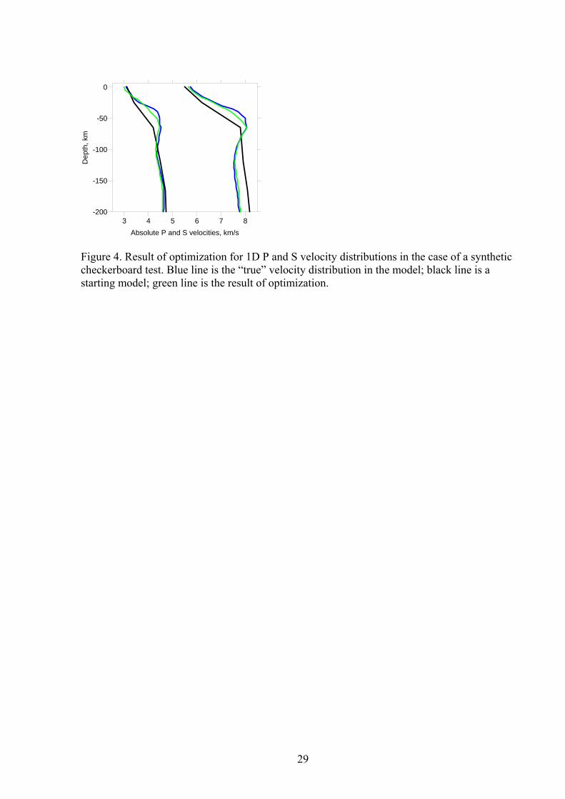
Figure 4. Result of optimization for 1D P and S velocity distributions in the case of a synthetic

checkerboard test. Blue line is the “true” velocity distribution in the model; black line is a

starting model; green line is the result of optimization.

Figure 5. Example of grid construction according to the ray density. The right-bottom map

shows the distribution of events (red dots) and stations (blue triangles). Grey lines indicate the

paths of S rays in the depth interval of 15-30 km. The four left maps show the plots of

normalized S ray density at 14, 19, 24, and 29 km depth. Dots are the parameterization nodes in

the depth interval of 5 km around the corresponding depth. Blue triangles indicate active

volcanoes. Presented is an example for an S model with a grid orientation of 45 degrees.

21

Figure 6. P and S velocity anomalies in horizontal sections obtained as a result of real data

inversion. The anomalies are given in percent with respect to the 1D model obtained as a result

of optimization. White contour lines within the “red” area indicate the levels of 10% and 20%

anomalies. Black dots indicate the final locations of sources in a corresponding depth interval.

Red triangles show positions of active volcanoes. Positions of the profiles for the cross sections

in Figure 7 are given in the plots for 5 km depth.

690

695

700

705

710

715

720

Figure 7. P and S velocity anomalies obtained as a result of real data inversion presented in two

vertical sections. Positions of sections are shown in Figure 6. The anomalies are given in percent

with respect to the 1D model obtained as a result of optimization. Blue triangles indicate

projections of stations located inside a 40 km range to the cross sections. Black dots indicate the

final locations of sources after executing 5 iterations located at distances less than 40 km from

the cross sections.

Figure 8. Inversion results for P and S models based on two independent data subsets (odd/even

test) presented in horizontal sections. Two left and two right columns represent the results for

subsets with odd and even events, respectively. Comparison of these results shows the robustness

of the results toward random factors (picking error, mainly).

Figure 9. Reconstruction of the checkerboard synthetic model. Synthetic anomalies are

represented by vertically non-limited alternated columns with lateral size of 30 km and

amplitudes of ±7%.The modeling conditions are described in the text. P and S results are

presented in horizontal sections.

Figure 10. Test for checking the vertical resolution. The initial model is shown in the upper row

both in map view and in cross sections, the same as for presenting the main results. The

conditions of the modeling are described in the text. Amplitudes of anomalies are ±7%. This test

aimed at checking the capacity of the algorithm to reconstruct the interface of the sign change at

40 km depth. It can be seen that the vertical resolution provided by the dataset is much lower

than the horizontal resolution demonstrated in Figure 9.

Figure 11. Synthetic model SYN2_sm1, which reproduces the images and values of formal

parameters as in the real case. The configurations of the P and S velocity anomalies in the model

are presented in horizontal sections in the left two columns. Numbers indicate the values of

velocity anomalies in the model. The right two columns represent the reconstruction results after

22

executing forward and inverse problems for the presented model. Conditions for performing the

modeling and the strategy for defining the synthetic model are described in the text.

Figure 12. Model SYN2_sm1 and reconstruction results as shown in Figure 11, but presented in

two vertical sections, as was used for presenting the results in Figure 7. Rows 1 and 3 represent P

and S models, respectively; rows 2 and 4 are the reconstruction results. Black dots are the

positions of sources in the starting model and in the final results. Blue triangles show the stations

projected to the cross sections.

725

730

735

740

745

750

755

Figure 13. Reconstruction of model SYN3_sm1, which is the same as SYN2_sm1 (Figures 11, 12)

in the depth interval of 0-40 km, but homogeneous in the deeper sections. The indications are the

same as in Figure 12. It can be seen that the crustal anomalies are strongly smeared downwards,

and the reconstruction results are hardly distinguishable from those in Figure 12.

Figure 14. Interpretation of the results along the Profile 1, same as in Figure 7. Background is the

distribution of P velocity anomalies. Yellow stars are the final location of events used in this

study. Blue, violet and red drops mark schematically the path of ascending fluids and partially

molten material.

Figure 15. Interpretation of the tomographic results for Central Java (Koulakov et al., in

preparation). The background is the result for P velocities along a vertical SN profile across Mt.

Merapi. Yellow stars show the distribution of local seismicity recorded within this study. The

pink ellipse highlights the events in the slab at 80 km – 120 km depth, which could be related to

phase transition and fluid release from the slab. Small blue and dark red circles indicate possible

distributions of released fluids and partial melting zones, respectively. The shallow green area to

the right of Merapi indicates the sediment cover above the MLA. Black strokes above the slab

indicate possible areas with higher stress concentrations.

Figure 16. P and S velocity anomalies in horizontal and vertical sections for Northern Chile

obtained using the LOTOS algorithm (similar to the results in Koulakov et al., 2006). Red

triangles in the map view indicate locations of volcanoes (Simkin and Siebert, 1994). Black dots

in the cross sections are the locations of events. Right – bottom plot is a cartoon interpreting the

results.

23

References: Aldiss, D. T. & Ghazali, S. A. (1984). The regional geology and evolution of the Toba volcano-

tectonic depression, Indonesia. Journal of the Geological Society, London 141, 487-500.

Chesner, C.A. and W.I.Rose (1991) Stratigraphy of the Toba Tuffs and the evolution of the Toba

Caldera Complex, Sumatra, Indonesia, Bulletin of Volcanology, Volume 53, Issue 5, pp 343-

356, DOI - 10.1007/BF00280226

Chesner, C. A., Rose, W. I., Deino, A. & Drake, R. (1991). Eruptive history of Earth's largest

Quaternary caldera (Toba, Indonesia) clarified. Geology 19, 200-203.

DeMets, C., R. Gordon, D. Argus, and S. Stein, (1990), Current plate motions, Geophys. J. Int.,

101, 425-478.

Diehl, J. F., Onstott, T. C., Chesner, C. A. & Knight, M. D. (1987). No short reversals of

Brunhes age recorded in the Toba tuffs, north Sumatra, Indonesia. Geophysical Research

Letters 14(7), 753-756.

Fauzi, R. McCaffrey, D. Wark, Sunaryo & P.Y. Prih Haryadi (1996), Lateral variation in slab

orientation beneath Toba caldera, Geophys. Res. Letters, 23, 443-446.

Kissling, E., W.Ellsworth, D.Eberhard-Phillips, and U.Kradolfer, (1994), Initial reference

models in local earthquake tomography, J.Geophys. Res. 99, 19.635-19.646,

Koulakov I., M. Bohm, G. Asch, B.-G. Lühr, A.Manzanares, K.S. Brotopuspito, Pak Fauzi, M.

A. Purbawinata, N.T. Puspito, A. Ratdomopurbo, H.Kopp, W. Rabbel, E.Shevkunova

(2007), P and S velocity structure of the crust and the upper mantle beneath central Java from

local tomography inversion, J. Geophys. Res., 112, B08310, doi:10.1029/2006JB004712.

Koulakov, I., S.V.Sobolev, and G. Asch, (2006), P- and S-velocity images of the lithosphere-

asthenosphere system in the Central Andes from local-source tomographic inversion,

Geophys. Journ. Int., 167, 106-126.

Koulakov, I., and S. Sobolev, (2006), Moho depth and three-dimensional P and S structure of the

crust and uppermost mantle in the Eastern Mediterranean and Middle East derived from

tomographic inversion of local ISC data. Geophysical Journal International, Vol. 164, issue

1, p. 218-235.

Masturyono, R. McCaffrey, D. A. Wark, S. W. Roecker, Fauzi, G. Ibrahim, and Sukhyar, (2001),

Distribution of magma beneath Toba Caldera, North Sumatra, Indonesia, Constrained by 3-

dimensional P-wave velocities, seismicity, and gravity data, Geochemistry, Geophysics &

Geosystems, 2001, vol. 2.

24

25

Nakajima, J., T. Matsuzawa, A. Hasegawa, and D. Zhao, (2001), Three-dimensional structure of

Vp, Vs and Vp/Vs beneath northeastern Japan: Implication for arc magmatism and fluids,

J.Geophys.Res., 106, 21843-21857.

Ninkovich, D., Shackleton, N. J., Abdel-Monem, A. A., Obradovich, J. D. & Izett, G. (1978). K-

Ar age of the late Pleistocene eruption of Toba, north Sumatra. Nature 276, 574-577.

Nishimura, S., Abe, E., Yokoyama, T., Wirasantosa, S. & Dharma, A. (1977). Danau Toba-the

outline of Lake Toba, North Sumatra, Indonesia. Paleolimnology Lake Biwa and the

Japanese Pleistocene 5, 313-332.

Nolet, G. (1981), Linearized inversion of (teleseismic) data. In R. Cassinis (ed.), editor, The

solution of the inverse problem in geophysical interpretation, pages 9-37. Plenum Press,.

Paige, C.C., and M.A. Saunders, (1982), LSQR: An algorithm for sparse linear equations and

sparse least squares, ACM trans. Math. Soft., 8, 43-71.

Poli, S., and M.W. Schmidt, (1995), H2O transport and release in subduction zones:

Experimental constrains on basaltic and andesitic systems, J.Geophys. Res., 100, 22299-

22314.

Pulunggono, A. & Cameron, N. R. (1984). Sumatran microplates, their characteristics and their

role in the evolution of the Central and South Sumatra basins. Proceedings of the Indonesian

Petroleum Association. 13, 121-143.

Rose, W. I. & Chesner, C. A. (1987). Dispersal of ash in the great Toba eruption, 75 ka. Geology

15, 913-917.

Simkin T., and L. Siebert, (1994),Volcanoes of the World, 2nd edition: Geoscience Press in

association with the Smithsonian Institution Global Volcanism Program, Tucson AZ, 368 p.

Smith, R. L. & Bailey, R. A. (1968). Resurgent cauldrons. In: Coats, R. R., Hay, R. L. &

Anderson, C. A. (eds) Studies in Volcanology. Geological Society of America, Memoir 116,

613-662.

Um, J., and Thurber, (1987), A fast algorithm for two-point seismic ray tracing, Bull.Seism. Soc.

Am., 77, 972-986,

Van Bemmelen, R. W. (1949). The geology of Indonesia. In: General Geology of Indonesia and

Adjacent Archipelagos, 1A. The Hague: Government Printing Office, 732 pp.

Van der Sluis, A., and H.A. van der Vorst, (1987), Numerical solution of large, sparse linear

algebraic systems arising from tomographic problems, in: Seismic tomography, edited by

G.Nolet, pp. 49-83, Reidel, Dortrecht,

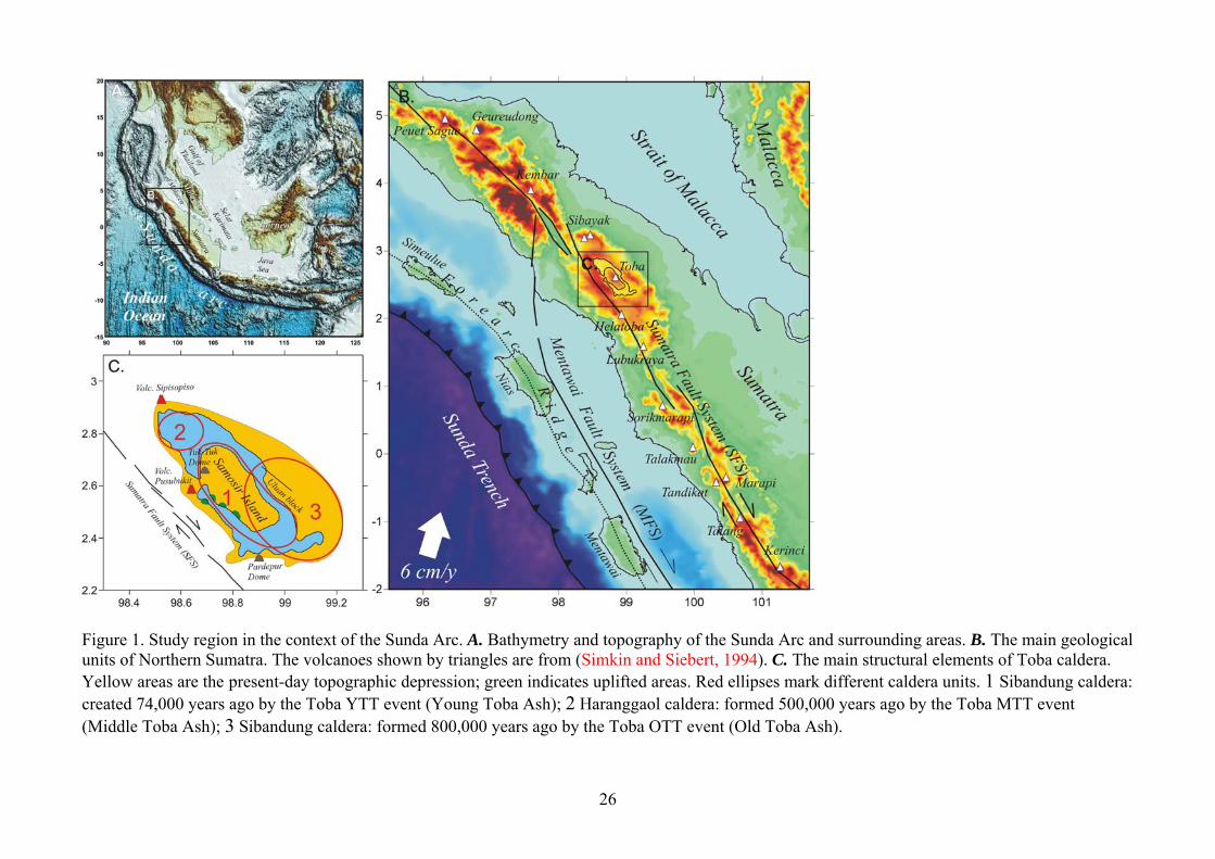
Figure 1. Study region in the context of the Sunda Arc. A. Bathymetry and topography of the Sunda Arc and surrounding areas. B. The main geological units of Northern Sumatra. The volcanoes shown by triangles are from (Simkin and Siebert, 1994). C. The main structural elements of Toba caldera. Yellow areas are the present-day topographic depression; green indicates uplifted areas. Red ellipses mark different caldera units. 1 Sibandung caldera: created 74,000 years ago by the Toba YTT event (Young Toba Ash); 2 Haranggaol caldera: formed 500,000 years ago by the Toba MTT event (Middle Toba Ash); 3 Sibandung caldera: formed 800,000 years ago by the Toba OTT event (Old Toba Ash).

26

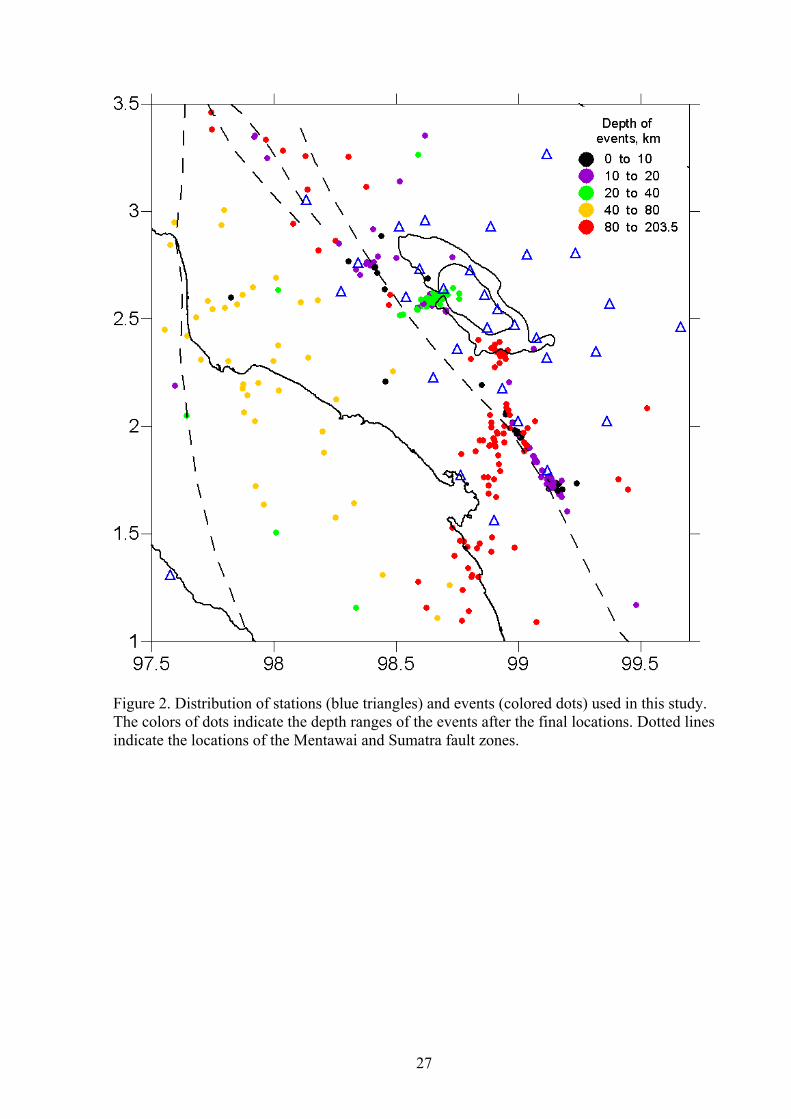
Figure 2. Distribution of stations (blue triangles) and events (colored dots) used in this study. The colors of dots indicate the depth ranges of the events after the final locations. Dotted lines indicate the locations of the Mentawai and Sumatra fault zones.

27

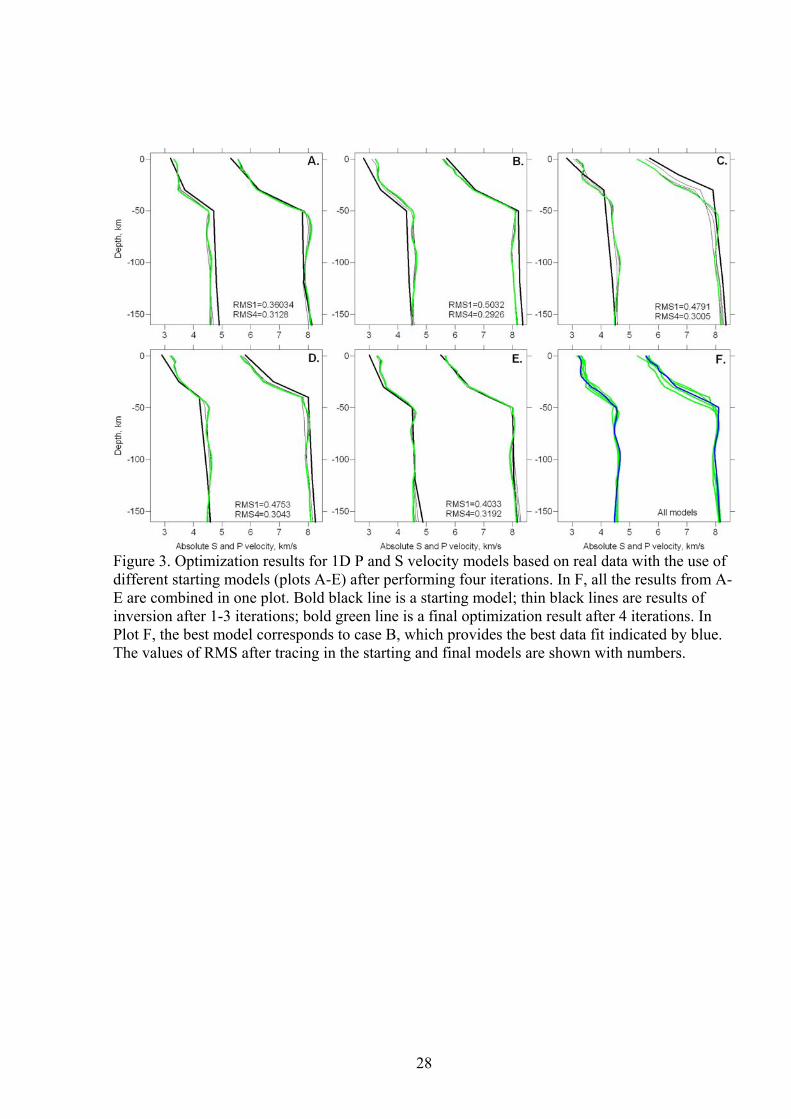
Figure 3. Optimization results for 1D P and S velocity models based on real data with the use of different starting models (plots A-E) after performing four iterations. In F, all the results from A-E are combined in one plot. Bold black line is a starting model; thin black lines are results of inversion after 1-3 iterations; bold green line is a final optimization result after 4 iterations. In Plot F, the best model corresponds to case B, which provides the best data fit indicated by blue. The values of RMS after tracing in the starting and final models are shown with numbers.

28

3 4 5 6 7 8Absolute P and S velocities, km/s

-200

-150

-100

-50

0D

epth

, km

Figure 4. Result of optimization for 1D P and S velocity distributions in the case of a synthetic checkerboard test. Blue line is the “true” velocity distribution in the model; black line is a starting model; green line is the result of optimization.

29

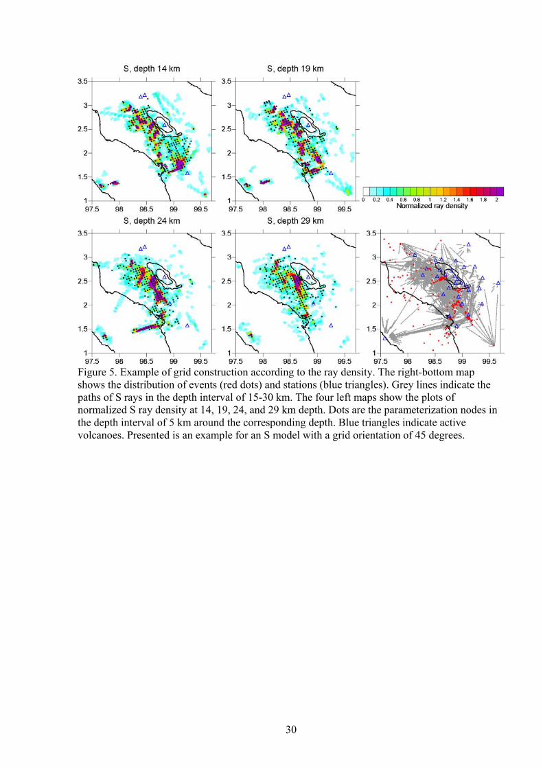
Figure 5. Example of grid construction according to the ray density. The right-bottom map shows the distribution of events (red dots) and stations (blue triangles). Grey lines indicate the paths of S rays in the depth interval of 15-30 km. The four left maps show the plots of normalized S ray density at 14, 19, 24, and 29 km depth. Dots are the parameterization nodes in the depth interval of 5 km around the corresponding depth. Blue triangles indicate active volcanoes. Presented is an example for an S model with a grid orientation of 45 degrees.

30

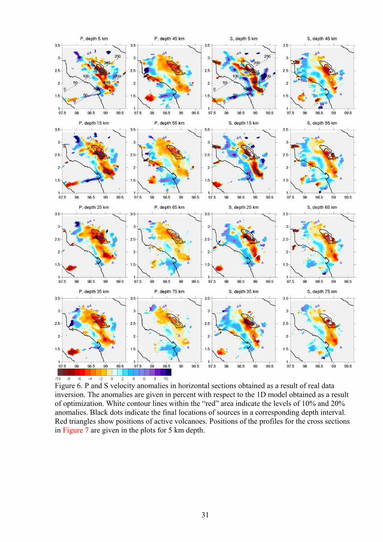
Figure 6. P and S velocity anomalies in horizontal sections obtained as a result of real data inversion. The anomalies are given in percent with respect to the 1D model obtained as a result of optimization. White contour lines within the “red” area indicate the levels of 10% and 20% anomalies. Black dots indicate the final locations of sources in a corresponding depth interval. Red triangles show positions of active volcanoes. Positions of the profiles for the cross sections in Figure 7 are given in the plots for 5 km depth.

31

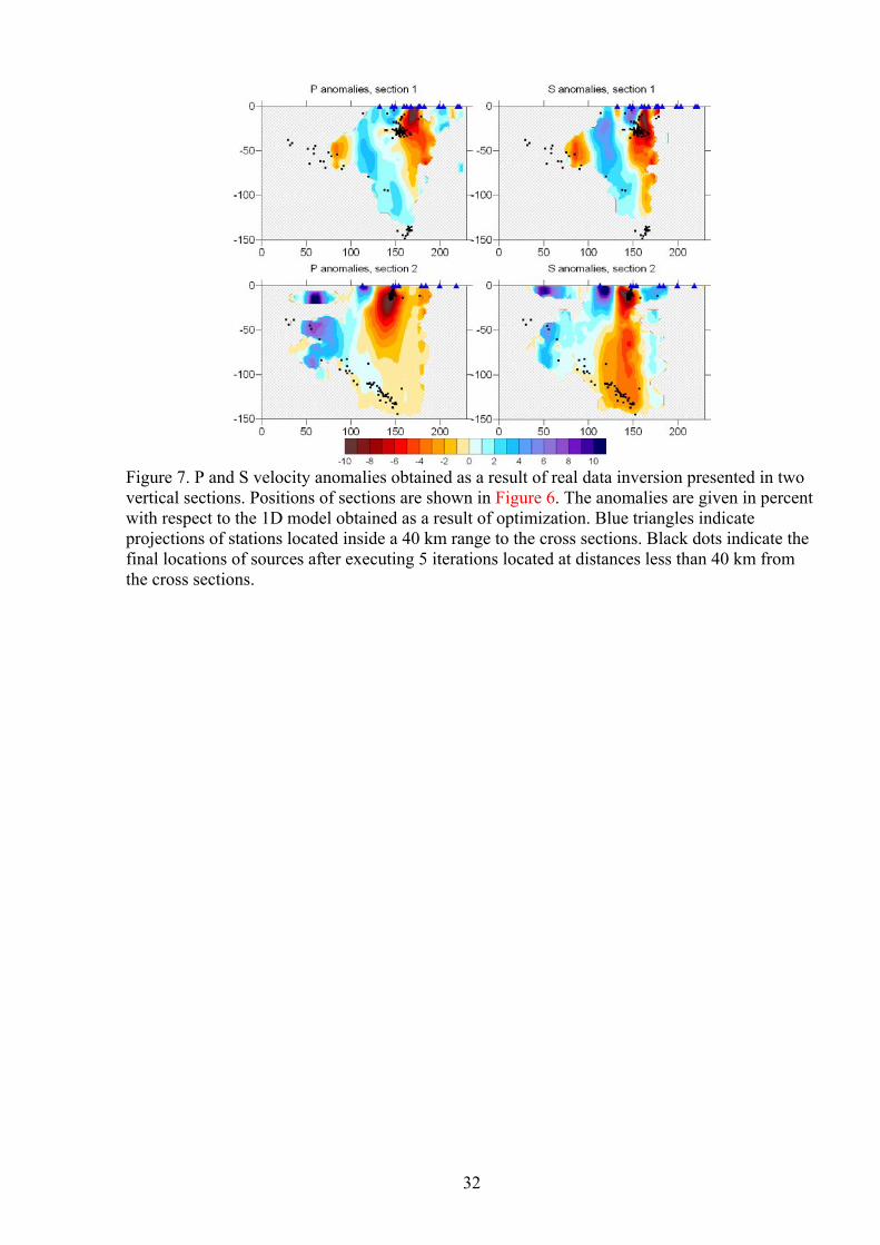
Figure 7. P and S velocity anomalies obtained as a result of real data inversion presented in two vertical sections. Positions of sections are shown in Figure 6. The anomalies are given in percent with respect to the 1D model obtained as a result of optimization. Blue triangles indicate projections of stations located inside a 40 km range to the cross sections. Black dots indicate the final locations of sources after executing 5 iterations located at distances less than 40 km from the cross sections.

32

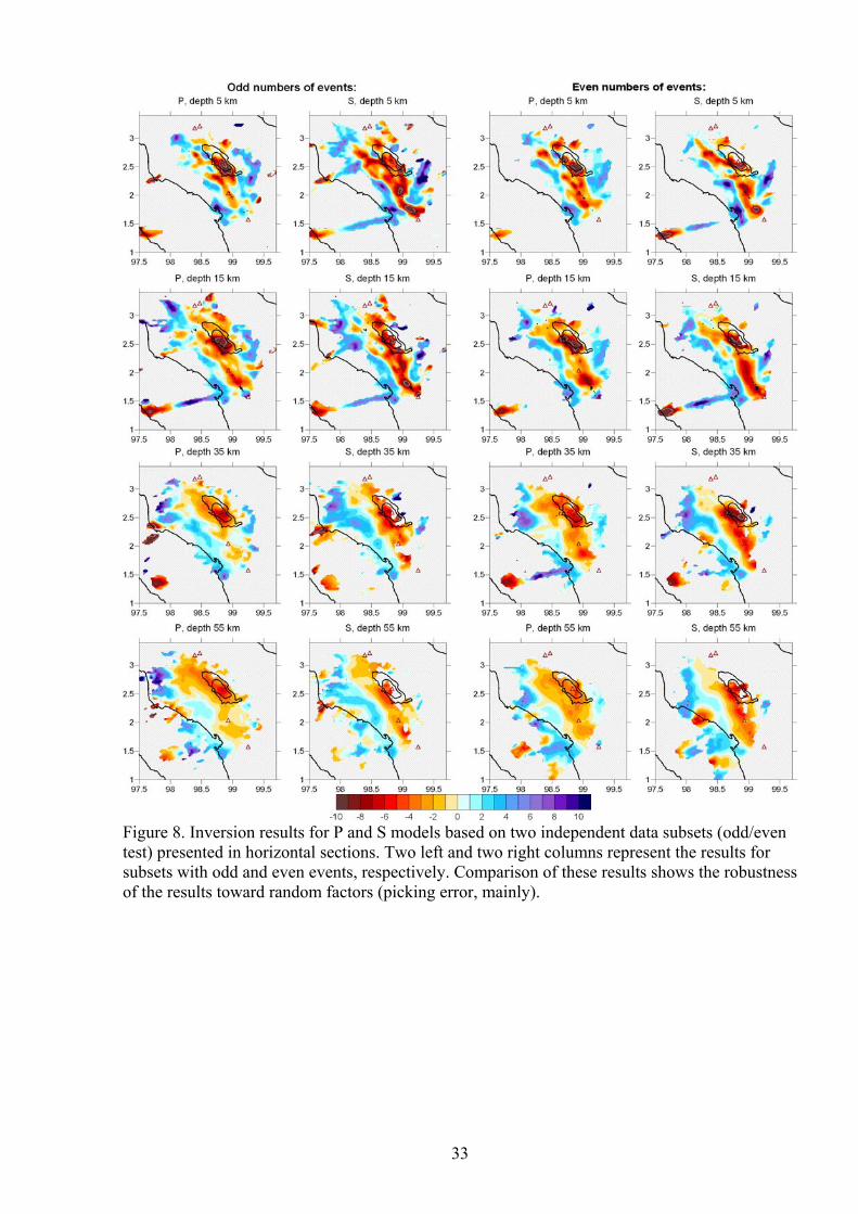
Figure 8. Inversion results for P and S models based on two independent data subsets (odd/even test) presented in horizontal sections. Two left and two right columns represent the results for subsets with odd and even events, respectively. Comparison of these results shows the robustness of the results toward random factors (picking error, mainly).

33

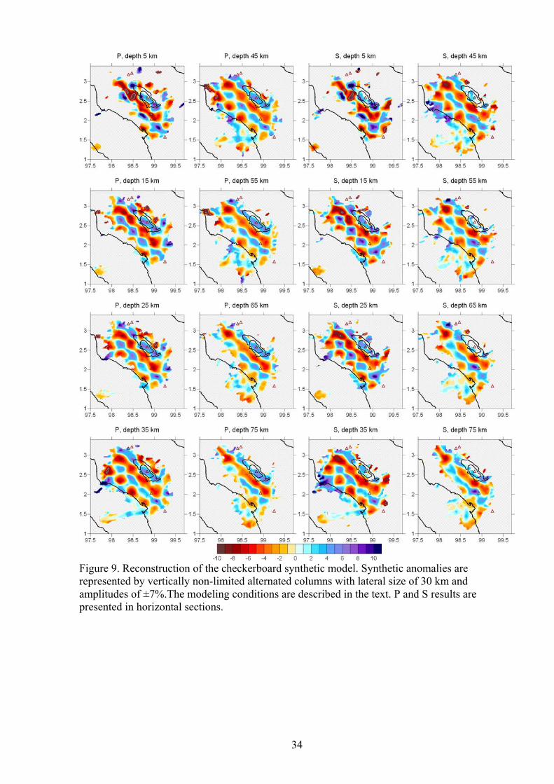
Figure 9. Reconstruction of the checkerboard synthetic model. Synthetic anomalies are represented by vertically non-limited alternated columns with lateral size of 30 km and amplitudes of ±7%.The modeling conditions are described in the text. P and S results are presented in horizontal sections.

34

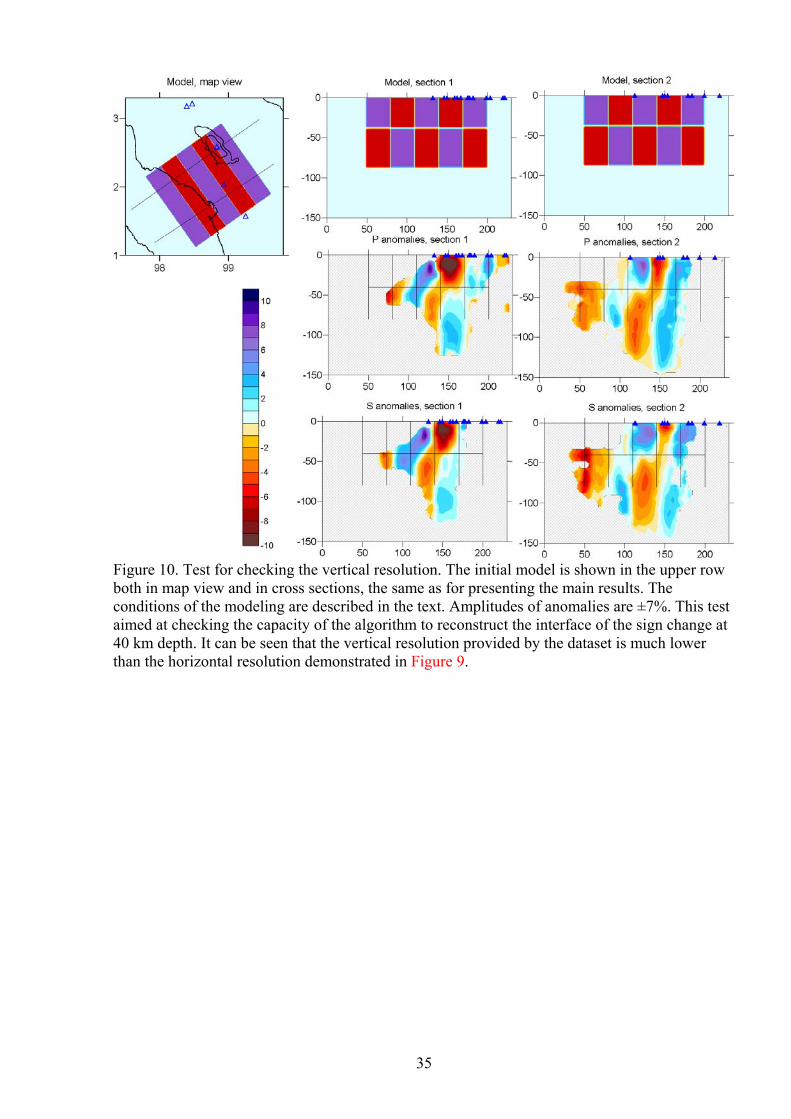
Figure 10. Test for checking the vertical resolution. The initial model is shown in the upper row both in map view and in cross sections, the same as for presenting the main results. The conditions of the modeling are described in the text. Amplitudes of anomalies are ±7%. This test aimed at checking the capacity of the algorithm to reconstruct the interface of the sign change at 40 km depth. It can be seen that the vertical resolution provided by the dataset is much lower than the horizontal resolution demonstrated in Figure 9.

35

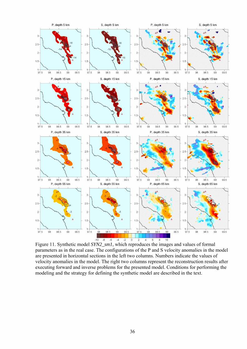
Figure 11. Synthetic model SYN2_sm1, which reproduces the images and values of formal parameters as in the real case. The configurations of the P and S velocity anomalies in the model are presented in horizontal sections in the left two columns. Numbers indicate the values of velocity anomalies in the model. The right two columns represent the reconstruction results after executing forward and inverse problems for the presented model. Conditions for performing the modeling and the strategy for defining the synthetic model are described in the text.

36

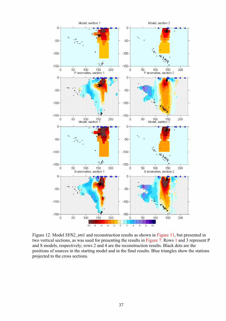
Figure 12. Model SYN2_sm1 and reconstruction results as shown in Figure 11, but presented in two vertical sections, as was used for presenting the results in Figure 7. Rows 1 and 3 represent P and S models, respectively; rows 2 and 4 are the reconstruction results. Black dots are the positions of sources in the starting model and in the final results. Blue triangles show the stations projected to the cross sections.

37

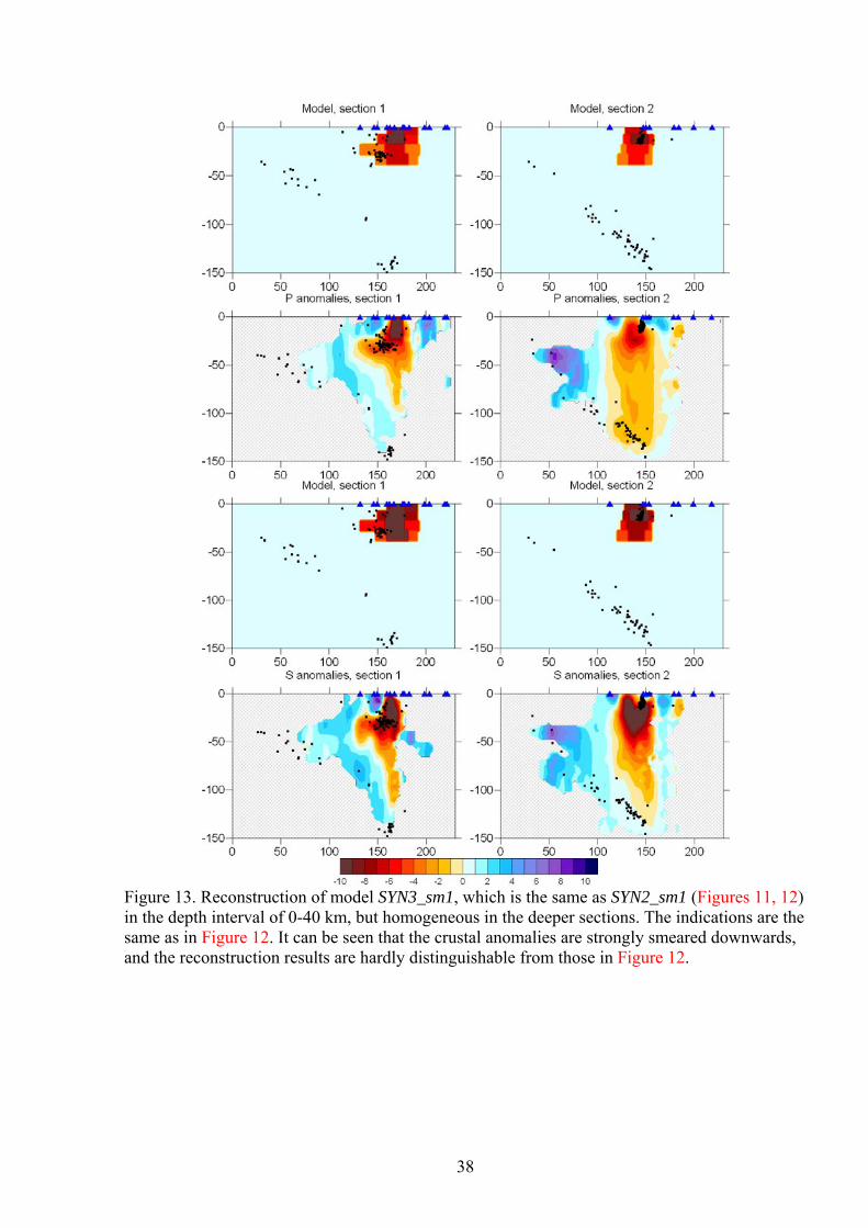
Figure 13. Reconstruction of model SYN3_sm1, which is the same as SYN2_sm1 (Figures 11, 12) in the depth interval of 0-40 km, but homogeneous in the deeper sections. The indications are the same as in Figure 12. It can be seen that the crustal anomalies are strongly smeared downwards, and the reconstruction results are hardly distinguishable from those in Figure 12.

38

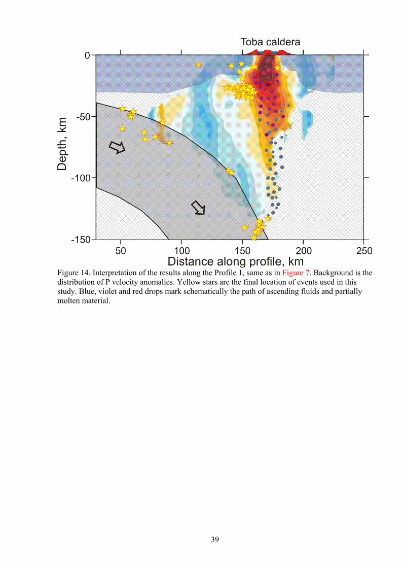
Figure 14. Interpretation of the results along the Profile 1, same as in Figure 7. Background is the distribution of P velocity anomalies. Yellow stars are the final location of events used in this study. Blue, violet and red drops mark schematically the path of ascending fluids and partially molten material.

39

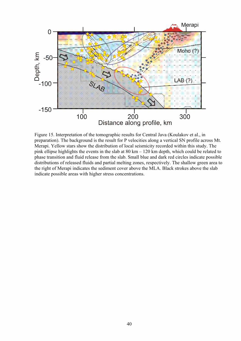
Figure 15. Interpretation of the tomographic results for Central Java (Koulakov et al., in preparation). The background is the result for P velocities along a vertical SN profile across Mt. Merapi. Yellow stars show the distribution of local seismicity recorded within this study. The pink ellipse highlights the events in the slab at 80 km – 120 km depth, which could be related to phase transition and fluid release from the slab. Small blue and dark red circles indicate possible distributions of released fluids and partial melting zones, respectively. The shallow green area to the right of Merapi indicates the sediment cover above the MLA. Black strokes above the slab indicate possible areas with higher stress concentrations.

40

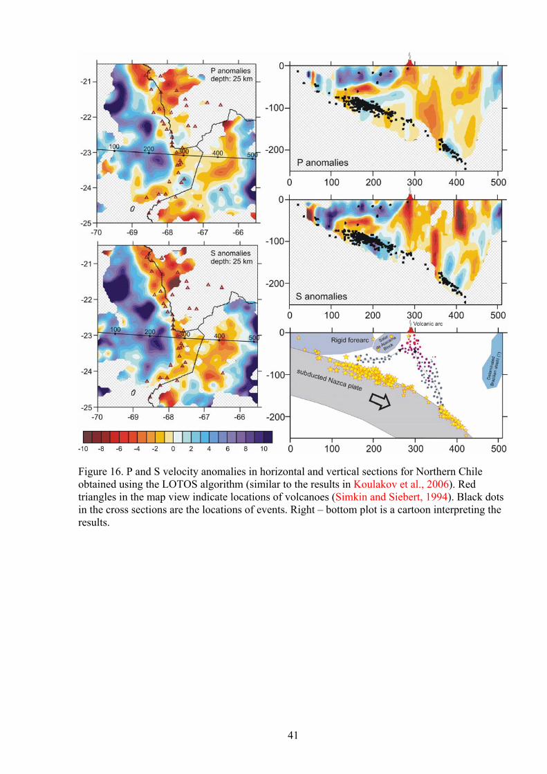
Figure 16. P and S velocity anomalies in horizontal and vertical sections for Northern Chile obtained using the LOTOS algorithm (similar to the results in Koulakov et al., 2006). Red triangles in the map view indicate locations of volcanoes (Simkin and Siebert, 1994). Black dots in the cross sections are the locations of events. Right – bottom plot is a cartoon interpreting the results.

41