Overview of the observation usage in the ALADIN ...
35
Overview of the observation usage in the ALADIN variational data assimilation system Sándor Kertész RC LACE Data Manager Hungarian Meteorological Service [email protected] 11 th June, 2007
Transcript of Overview of the observation usage in the ALADIN ...
Overview of the observation usage in the ALADIN
variational data assimilation system
Sándor KertészRC LACE Data Manager
Hungarian Meteorological [email protected]
11th June, 2007
Table of Contents
1 Preface...............................................................................................................................................32 General overview of the data assimilation system.............................................................................4
2.1 Observation pre-processing........................................................................................................42.2 Variational analysis ....................................................................................................................62.3 Surface analysis by CANARI.....................................................................................................7
3 Observation types..............................................................................................................................83.1 Observation types and parameters..............................................................................................83.2 SYNOP observations..................................................................................................................93.3 AIREP observations...................................................................................................................93.4 SATOB observations..................................................................................................................93.5 TEMP observations..................................................................................................................103.6 PILOT.......................................................................................................................................103.7 SATEM ....................................................................................................................................10
4 The OBSOUL file format................................................................................................................124.1 SYNOP......................................................................................................................................134.2 AIREP.......................................................................................................................................134.3 SATOB......................................................................................................................................144.4 TEMP........................................................................................................................................154.5 PILOT.......................................................................................................................................164.6 SATEM.....................................................................................................................................17
5 Producing the OBSOUL file...........................................................................................................205.1 Programme OULAN_hms........................................................................................................20
5.1.1 The structure of OULAN_hms...........................................................................................205.1.2 Observation usage in OULAN_hms..................................................................................205.1.3 Running OULAN_hms......................................................................................................21
6 Programme BATOR........................................................................................................................246.1 How to run BATOR..................................................................................................................246.2 Observation errors....................................................................................................................246.3 File ficdate................................................................................................................................256.4 File refdata................................................................................................................................256.5 File BATOR_MAP...................................................................................................................256.6 Blacklisting ..............................................................................................................................26
6.6.1 File LISTE_NOIRE_DIAP................................................................................................266.6.2 File LISTE_LOC ..............................................................................................................27
6.7 Observation files.......................................................................................................................296.8 LAMFLAG filtering.................................................................................................................29
7 Observation control in screening.....................................................................................................317.1 Screening decisions...................................................................................................................317.2 Blacklisting................................................................................................................................317.3 Background quality control.......................................................................................................317.4 Thinning....................................................................................................................................327.5 Satellite radiance bias correction..............................................................................................337.6 Output statistics.........................................................................................................................33
8 Observation control in minimization ..............................................................................................349 References........................................................................................................................................3510 Acknowledgements........................................................................................................................35
2

1 Preface
This document was prepared to provide a general overview about the observation pre-processing and observation usage techniques in the ALADIN variational data assimilation system. This overview is based on the ALADIN 30 model version and basically reflects the experience gathered with the operational ALADIN data assimilation system at the Hungarian Meteorological Service (HMS).
Although ODB plays a central part in the presented processes it will not be discussed in detail since both training materials and advanced documentations are available in this topic. Besides, because CANARI is not used at HMS (although it can be used for surface analysis) little information will be provided about it.
Please note that this document can be regarded as a kind of compilation heavily relying on existing documentations (see the Chapter 9 for references).
3

2 General overview of the data assimilation system
The recent ALADIN data assimilation system comprises three main parts: observation pre-processing, variational analysis for the upper air fields (3D-VAR) and optimal interpolation analysis for the surface fields (CANARI, conf. 701). The 3D-VAR step consists of two further steps: at first the observation screening (quality control) takes place (conf. 002) and it is followed by the minimization step (conf. 131). The CANARI step is omitted in the operational practice (at Météo France and HMS) and replaced by simply taking the surface fields from the ARPEGE analysis.
Figure 1: General overview of the ALADIN variational data assimilation system (the CANARI step is omitted in the present operational practice)
2.1 Observation pre-processing
The main goal of the observation pre-processing is to provide the analysis procedure with the observations in ODB format. For more details and practical information about ODB please read [4] and [8].
At present all the 3 involved model configurations (002, 131, 701) require observations in ODB format. Two ODB formats are relevant to the ALADIN data assimilation: ECMA and CCMA. The CCMA format is a compressed version of ECMA. Screening and CANARI require an ECMA ODB while the minimization requires a CCMA one. Strictly speaking the observation pre-processing has to produce input ODBs only for screening and CANARI, because the input ODB for minimization is produced by the processing of the output ODB of screening.
The ECMA ODBs are produced by programme BATOR. BATOR also assigns the observation errors to the data and prepares blacklisting. At present, BATOR takes three kinds of input observation formats:
• ASCII: this is the so-called OBSOUL file produced by programme OULAN developed at MF. The original format of OULAN reads data from the local database of MF so it is not suitable for use at other sites. In order to use OULAN outside MF it has to be customized to the local observation
Screening (conf. 002)
Minimization (conf. 131)
CANARI (conf .701)
Analysis
Observation preprocessing
Surface analyis (oprtimal interpolation)
Upper air analyis (3DVAR)
Background (a forecast from the previous
analysis)
Statistics (background, observations)
Observations in ODB
4
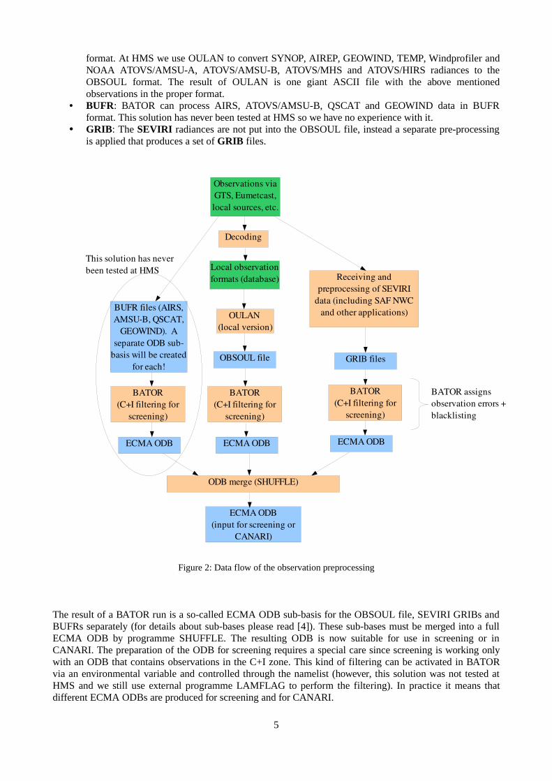
format. At HMS we use OULAN to convert SYNOP, AIREP, GEOWIND, TEMP, Windprofiler and NOAA ATOVS/AMSU-A, ATOVS/AMSU-B, ATOVS/MHS and ATOVS/HIRS radiances to the OBSOUL format. The result of OULAN is one giant ASCII file with the above mentioned observations in the proper format.
• BUFR: BATOR can process AIRS, ATOVS/AMSU-B, QSCAT and GEOWIND data in BUFR format. This solution has never been tested at HMS so we have no experience with it.
• GRIB: The SEVIRI radiances are not put into the OBSOUL file, instead a separate pre-processing is applied that produces a set of GRIB files.
Figure 2: Data flow of the observation preprocessing
The result of a BATOR run is a so-called ECMA ODB sub-basis for the OBSOUL file, SEVIRI GRIBs and BUFRs separately (for details about sub-bases please read [4]). These sub-bases must be merged into a full ECMA ODB by programme SHUFFLE. The resulting ODB is now suitable for use in screening or in CANARI. The preparation of the ODB for screening requires a special care since screening is working only with an ODB that contains observations in the C+I zone. This kind of filtering can be activated in BATOR via an environmental variable and controlled through the namelist (however, this solution was not tested at HMS and we still use external programme LAMFLAG to perform the filtering). In practice it means that different ECMA ODBs are produced for screening and for CANARI.
Decoding
OULAN (local version)
BATOR(C+I filtering for
screening)
Observations via GTS, Eumetcast, local sources, etc.
OBSOUL file
Local observation formats (database)
ECMA ODB
BATOR(C+I filtering for
screening)
ECMA ODB
GRIB files
Receiving and preprocessing of SEVIRI
data (including SAF NWC and other applications)
ODB merge (SHUFFLE)
ECMA ODB(input for screening or
CANARI)
BATOR(C+I filtering for
screening)
BUFR files (AIRS, AMSUB, QSCAT,
GEOWIND). A separate ODB sub
basis will be created for each!
ECMA ODB
BATOR assigns observation errors + blacklisting
This solution has never been tested at HMS
5
2.2 Variational analysis
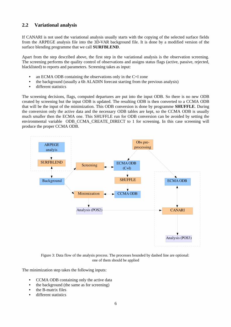
If CANARI is not used the variational analysis usually starts with the copying of the selected surface fields from the ARPEGE analysis file into the 3D-VAR background file. It is done by a modified version of the surface blending programme that we call SURFBLEND.
Apart from the step described above, the first step in the variational analysis is the observation screening. The screening performs the quality control of observations and assigns status flags (active, passive, rejected, blacklisted) to reports and parameters. Screening takes as input:
• an ECMA ODB containing the observations only in the C+I zone• the background (usually a 6h ALADIN forecast starting from the previous analysis)• different statistics
The screening decisions, flags, computed departures are put into the input ODB. So there is no new ODB created by screening but the input ODB is updated. The resulting ODB is then converted to a CCMA ODB that will be the input of the minimization. This ODB conversion is done by programme SHUFFLE. During the conversion only the active data and the necessary ODB tables are kept, so the CCMA ODB is usually much smaller then the ECMA one. This SHUFFLE run for ODB conversion can be avoided by setting the environmental variable ODB_CCMA_CREATE_DIRECT to 1 for screening. In this case screening will produce the proper CCMA ODB.
Figure 3: Data flow of the analysis process. The processes bounded by dashed line are optional: one of them should be applied
The minimization step takes the following inputs:
• CCMA ODB containing only the active data• the background (the same as for screening)• the B-matrix files• different statistics
Obs preprocessing
Screening SURFBLEND ECMA ODB
(C+I)
Analysis (POS2) CANARI
ARPEGE analyis
SHUFFLE
Minimization CCMA ODB
ECMA ODB
Analysis (POS3)
Background
6
All the computed departures, analysis increments and other information are put into the input ODB. So there is no new ODB created by the minimization but the input ODB is updated. The real result of the minimization step is the so called POS2 file that now contains the analysis for the upper air fields.
For more details about variational analysis please study [2] and [10].
2.3 Surface analysis by CANARI
The surface CANARI analysis takes the following inputs:
• an ECMA ODB containing the observations • the first guess (it is the POS2 file produced by 3D-VAR analysis)• different statistics
The quality control decisions (CANARI has its own quality control), flags, computed departures, surface increments etc. are put into the input ODB. So there is no new ODB created by CANARI but the input ODB is updated. The real result of CANARI is the so called POS3 file that is now contains both the upper air analysis (by 3D-VAR) and the surface analysis (by CANARI).
7
3 Observation types
In this chapter the different observation types, observed parameters and observing platforms will be presented briefly. I will mainly focus on the observations used in the ALADIN data assimilation system of HMS (other observations used outside HMS may not be mentioned at all).
3.1 Observation types and parameters
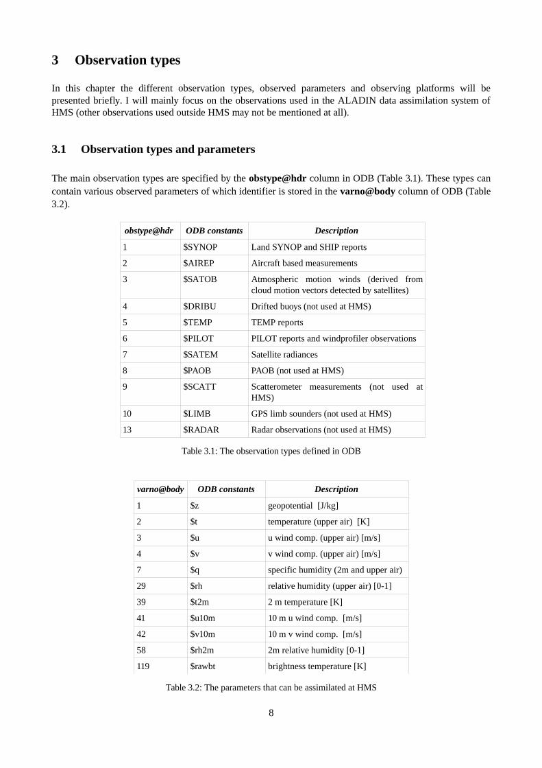
The main observation types are specified by the obstype@hdr column in ODB (Table 3.1). These types can contain various observed parameters of which identifier is stored in the varno@body column of ODB (Table 3.2).
obstype@hdr ODB constants Description
1 $SYNOP Land SYNOP and SHIP reports
2 $AIREP Aircraft based measurements
3 $SATOB Atmospheric motion winds (derived from cloud motion vectors detected by satellites)
4 $DRIBU Drifted buoys (not used at HMS)
5 $TEMP TEMP reports
6 $PILOT PILOT reports and windprofiler observations
7 $SATEM Satellite radiances
8 $PAOB PAOB (not used at HMS)
9 $SCATT Scatterometer measurements (not used at HMS)
10 $LIMB GPS limb sounders (not used at HMS)
13 $RADAR Radar observations (not used at HMS)
Table 3.1: The observation types defined in ODB
varno@body ODB constants Description
1 $z geopotential [J/kg]
2 $t temperature (upper air) [K]
3 $u u wind comp. (upper air) [m/s]
4 $v v wind comp. (upper air) [m/s]
7 $q specific humidity (2m and upper air)
29 $rh relative humidity (upper air) [0-1]
39 $t2m 2 m temperature [K]
41 $u10m 10 m u wind comp. [m/s]
42 $v10m 10 m v wind comp. [m/s]
58 $rh2m 2m relative humidity [0-1]
119 $rawbt brightness temperature [K]
Table 3.2: The parameters that can be assimilated at HMS
8
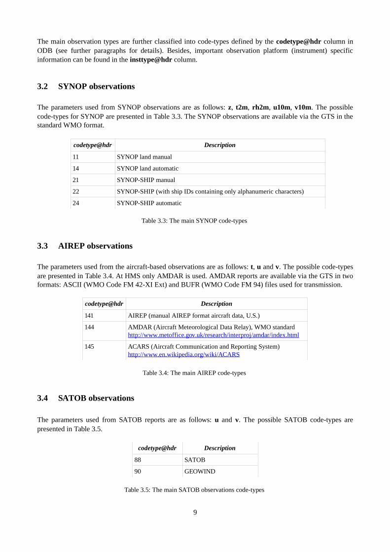
The main observation types are further classified into code-types defined by the codetype@hdr column in ODB (see further paragraphs for details). Besides, important observation platform (instrument) specific information can be found in the insttype@hdr column.
3.2 SYNOP observations
The parameters used from SYNOP observations are as follows: z, t2m, rh2m, u10m, v10m. The possible code-types for SYNOP are presented in Table 3.3. The SYNOP observations are available via the GTS in the standard WMO format.
codetype@hdr Description
11 SYNOP land manual
14 SYNOP land automatic
21 SYNOP-SHIP manual
22 SYNOP-SHIP (with ship IDs containing only alphanumeric characters)
24 SYNOP-SHIP automatic
Table 3.3: The main SYNOP code-types
3.3 AIREP observations
The parameters used from the aircraft-based observations are as follows: t, u and v. The possible code-types are presented in Table 3.4. At HMS only AMDAR is used. AMDAR reports are available via the GTS in two formats: ASCII (WMO Code FM 42-XI Ext) and BUFR (WMO Code FM 94) files used for transmission.
codetype@hdr Description
141 AIREP (manual AIREP format aircraft data, U.S.)
144 AMDAR (Aircraft Meteorological Data Relay), WMO standard http://www.metoffice.gov.uk/research/interproj/amdar/index.html
145 ACARS (Aircraft Communication and Reporting System) http://www.en.wikipedia.org/wiki/ACARS
Table 3.4: The main AIREP code-types
3.4 SATOB observations
The parameters used from SATOB reports are as follows: u and v. The possible SATOB code-types are presented in Table 3.5.
codetype@hdr Description
88 SATOB
90 GEOWIND
Table 3.5: The main SATOB observations code-types
9
The SATOB wind information is derived from a cloud motion detection process based on the measurements of geostationary satellites. At HMS only the GEOWIND (codetype=90) observations from MSG-1 (MSG-2 is also available) are used. It is available via the EUMETCAST dissemination system in BUFR format. Regarding the code-types the main difference between SATOB (88) and GEOWIND (90) is that in GEOWIND a QI (quality indicator) is available for the wind data.
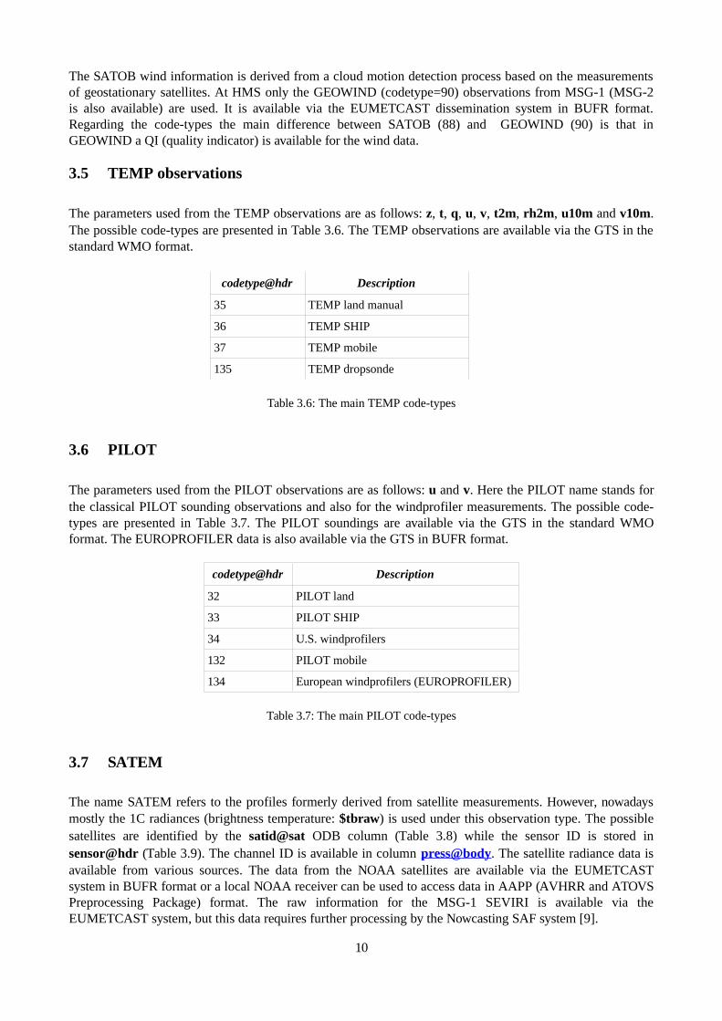
3.5 TEMP observations
The parameters used from the TEMP observations are as follows: z, t, q, u, v, t2m, rh2m, u10m and v10m. The possible code-types are presented in Table 3.6. The TEMP observations are available via the GTS in the standard WMO format.
codetype@hdr Description
35 TEMP land manual
36 TEMP SHIP
37 TEMP mobile
135 TEMP dropsonde
Table 3.6: The main TEMP code-types
3.6 PILOT
The parameters used from the PILOT observations are as follows: u and v. Here the PILOT name stands for the classical PILOT sounding observations and also for the windprofiler measurements. The possible code-types are presented in Table 3.7. The PILOT soundings are available via the GTS in the standard WMO format. The EUROPROFILER data is also available via the GTS in BUFR format.
codetype@hdr Description
32 PILOT land
33 PILOT SHIP
34 U.S. windprofilers
132 PILOT mobile
134 European windprofilers (EUROPROFILER)
Table 3.7: The main PILOT code-types
3.7 SATEM
The name SATEM refers to the profiles formerly derived from satellite measurements. However, nowadays mostly the 1C radiances (brightness temperature: $tbraw) is used under this observation type. The possible satellites are identified by the satid@sat ODB column (Table 3.8) while the sensor ID is stored in sensor@hdr (Table 3.9). The channel ID is available in column press@body. The satellite radiance data is available from various sources. The data from the NOAA satellites are available via the EUMETCAST system in BUFR format or a local NOAA receiver can be used to access data in AAPP (AVHRR and ATOVS Preprocessing Package) format. The raw information for the MSG-1 SEVIRI is available via the EUMETCAST system, but this data requires further processing by the Nowcasting SAF system [9].
10
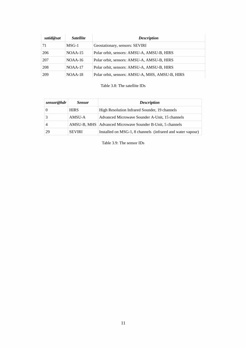
satid@sat Satellite Description
71 MSG-1 Geostationary, sensors: SEVIRI
206 NOAA-15 Polar orbit, sensors: AMSU-A, AMSU-B, HIRS
207 NOAA-16 Polar orbit, sensors: AMSU-A, AMSU-B, HIRS
208 NOAA-17 Polar orbit, sensors: AMSU-A, AMSU-B, HIRS
209 NOAA-18 Polar orbit, sensors: AMSU-A, MHS, AMSU-B, HIRS
Table 3.8: The satellite IDs
sensor@hdr Sensor Description
0 HIRS High Resolution Infrared Sounder, 19 channels
3 AMSU-A Advanced Microwave Sounder A-Unit, 15 channels
4 AMSU-B, MHS Advanced Microwave Sounder B-Unit, 5 channels
29 SEVIRI Installed on MSG-1, 8 channels (infrared and water vapour)
Table 3.9: The sensor IDs
11
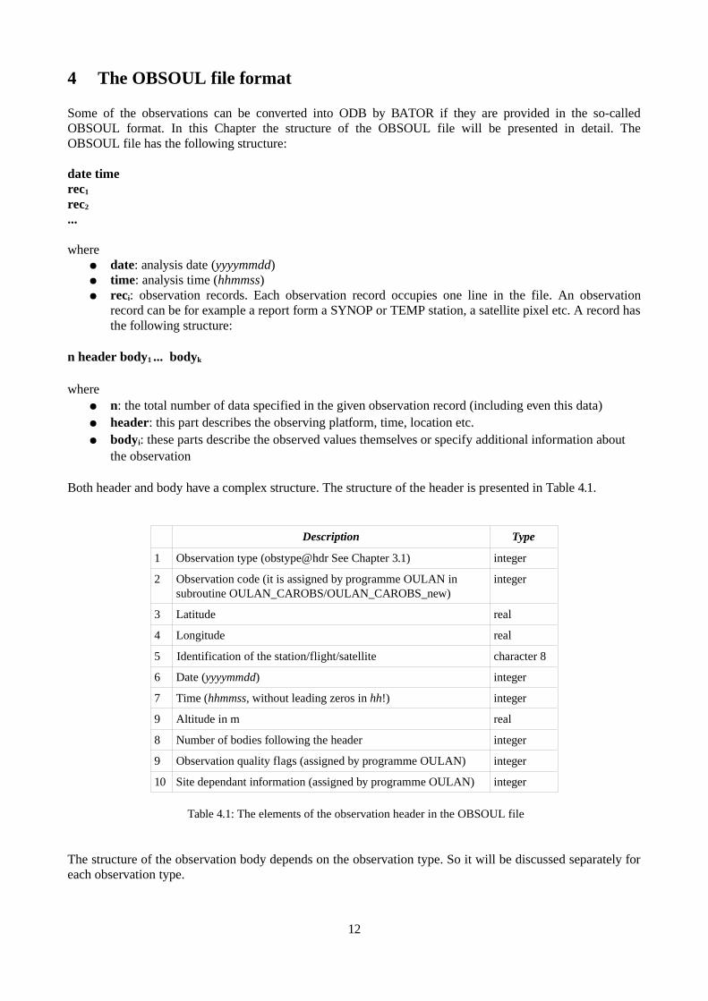
4 The OBSOUL file format
Some of the observations can be converted into ODB by BATOR if they are provided in the so-called OBSOUL format. In this Chapter the structure of the OBSOUL file will be presented in detail. The OBSOUL file has the following structure:
date timerec1
rec2
...
where ● date: analysis date (yyyymmdd)● time: analysis time (hhmmss)● reci: observation records. Each observation record occupies one line in the file. An observation
record can be for example a report form a SYNOP or TEMP station, a satellite pixel etc. A record has the following structure:
n header body1 ... bodyk
where● n: the total number of data specified in the given observation record (including even this data)● header: this part describes the observing platform, time, location etc. ● bodyi: these parts describe the observed values themselves or specify additional information about
the observation
Both header and body have a complex structure. The structure of the header is presented in Table 4.1.
Description Type
1 Observation type (obstype@hdr See Chapter 3.1) integer
2 Observation code (it is assigned by programme OULAN in subroutine OULAN_CAROBS/OULAN_CAROBS_new)
integer
3 Latitude real
4 Longitude real
5 Identification of the station/flight/satellite character 8
6 Date (yyyymmdd) integer
7 Time (hhmmss, without leading zeros in hh!) integer
9 Altitude in m real
8 Number of bodies following the header integer
9 Observation quality flags (assigned by programme OULAN) integer
10 Site dependant information (assigned by programme OULAN) integer
Table 4.1: The elements of the observation header in the OBSOUL file
The structure of the observation body depends on the observation type. So it will be discussed separately for each observation type.
12

4.1 SYNOP
SYNOP observation records describe SYNOP reports. So the header specifies the characteristics of the reporting station while bodies contain the observed values. In the present system z, t2, rhu2, q2, u10 and v10 can be assimilated from SYNOP reports.
Concerning the header the observation quality flags can be set to 1111 while the site dependant information should be set to 100000. These are the default values. The observation code can be read out from the OULAN_CAROBS subroutine of OULAN (it depends on the observation subtype too).
Body entries for SYNOP reports have the following structure:
description type
1 Parameter type (varid@body, See Chapter 3) integer
2 Vertical coordinate (fill value: 0.1699999976E+39) real
3 Fill value: 0.1699999976E+39 real
4 Observed value real
5 Parameter quality flag (assigned by OULAN) integer
Table 4.2: The observation body structure for SYNOP in the OBSOUL filewhere:
● The body elements of land SYNOPs and SHIPs are interpreted in a slightly different way. For land SYNOPs the vertical coordinate is the station level pressure in Pa. The exception is z for which if MSLP is available then it should be specified here with a minus sign (!) otherwise the station level pressure should be given. For SHIPs the MSLP and station level pressure are the same so here for the vertical coordinate a fill value should be specified. The only exception is z for which MSLP must be given with a minus sign (!).
● For the 3rd body entry a fill value is specified. The only exception is the q2 where the observation error computed by OULAN in subroutine EXT_LAM_SYNOP should be given here.
● For z the observed value should be set to 0 if the MSLP is specified. In any other case it should be set to the station altitude multiplied by g.
● For the wind the speed and direction are stored in the OBSOUL file instead of the u and v components. Thus for the 10 m wind only one body entry (for parameter 41) is specified having the wind speed in position 3 and the wind direction (in degrees) in position 4.
● The parameter quality flag should be set to 2064 in the case of z and to 2048 for the rest of the parameters.
An example of a land SYNOP observation record is specified below:
42 1 10014011 48.10000 19.51667 '12756 ' 20041215 120000 153.0000000 6 1111 100000 1 -103290.0000 0.1699999976E+39 0.0000000000E+00 2064 39 101310.0000 0.1699999976E+39 271.2600098 2048 58 101310.0000 0.1699999976E+39 82.00000000 2048 7 101310.0000 0.3211538133E-03 0.2632536227E-02 2048 41 101310.0000 3.000000000 190.0000000 2048 91 101310.0000 0.1699999976E+39 100.0000000 2048
4.2 AIREP
AIREP observation records describe aircraft measurements within a flight. Thus one flight consists of several observation reports. The header specifies the characteristics of the report (location, time and flight
13

ID) while bodies contain the observed values. In the present system t, u and v can be assimilated from AIREP reports.
Concerning the header the observation quality flags should be set to 11111 while the site dependant information should be set to 0. These are the default values. The observation code can be read out from the OULAN_CAROBS subroutine of OULAN (it depends on the observation subtype too).
Body entries for AIREP reports have the following structure:
description type
1 Parameter type (varid@body, See Chapter 3) integer
2 Vertical coordinate (fill value: 0.1699999976E+39) real
3 Fill value: 0.1699999976E+39 real
4 Observed value real
5 Parameter quality flag (assigned by OULAN) integer
Table 4.3: The observation body structure for AIREP in the OBSOUL file
where:
● The vertical coordinate is the pressure level of the observation in Pa. ● For the wind the speed and direction are stored in the OBSOUL file instead of the u and v
components Thus for the wind only one body entry (for parameter 3) is specified having the wind speed in position 3 and the wind direction (in degrees) in position 4.
● The parameter quality flag should be set to 4111 both for t and wind.
An example of an AIREP observation record is specified below:
22 2 10061144 56.73000 -3.10000 'EU0807 ' 20050518 85700 4846.319824 2 11111 0 2 4846.319824 0.1699999976E+39 248.4600067 4111 3 4846.319824 11.31000042 300.0000000 4111
4.3 SATOB
A SATOB observation record/report describes one upper air observation at a given spatial location. The header specifies the characteristics of the report (location, time and satellite ID) while bodies contain the quality indicator information and the observed values. In the present system u and v can be assimilated from SATOB reports.
Concerning the header the observation quality flags should be set to 11111 while the site dependant information should be set to 0. These are the default values. The observation code can be read out from the OULAN_CAROBS_new subroutine of OULAN (it depends on the observation subtype too).
The first body entry for SATOB always contains information about the quality of the measurement. It has the following structure:
14
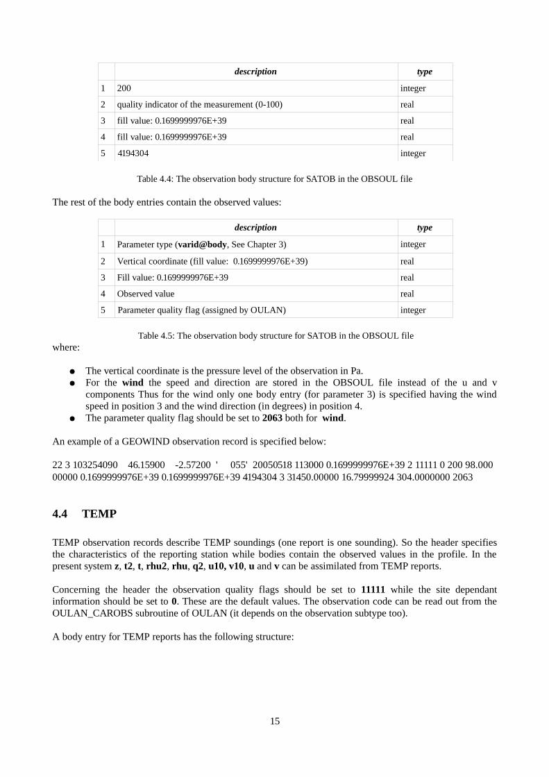
description type
1 200 integer
2 quality indicator of the measurement (0-100) real
3 fill value: 0.1699999976E+39 real
4 fill value: 0.1699999976E+39 real
5 4194304 integer
Table 4.4: The observation body structure for SATOB in the OBSOUL file
The rest of the body entries contain the observed values:
description type
1 Parameter type (varid@body, See Chapter 3) integer
2 Vertical coordinate (fill value: 0.1699999976E+39) real
3 Fill value: 0.1699999976E+39 real
4 Observed value real
5 Parameter quality flag (assigned by OULAN) integer
Table 4.5: The observation body structure for SATOB in the OBSOUL filewhere:
● The vertical coordinate is the pressure level of the observation in Pa. ● For the wind the speed and direction are stored in the OBSOUL file instead of the u and v
components Thus for the wind only one body entry (for parameter 3) is specified having the wind speed in position 3 and the wind direction (in degrees) in position 4.
● The parameter quality flag should be set to 2063 both for wind.
An example of a GEOWIND observation record is specified below:
22 3 103254090 46.15900 -2.57200 ' 055' 20050518 113000 0.1699999976E+39 2 11111 0 200 98.00000000 0.1699999976E+39 0.1699999976E+39 4194304 3 31450.00000 16.79999924 304.0000000 2063
4.4 TEMP
TEMP observation records describe TEMP soundings (one report is one sounding). So the header specifies the characteristics of the reporting station while bodies contain the observed values in the profile. In the present system z, t2, t, rhu2, rhu, q2, u10, v10, u and v can be assimilated from TEMP reports.
Concerning the header the observation quality flags should be set to 11111 while the site dependant information should be set to 0. These are the default values. The observation code can be read out from the OULAN_CAROBS subroutine of OULAN (it depends on the observation subtype too).
A body entry for TEMP reports has the following structure:
15
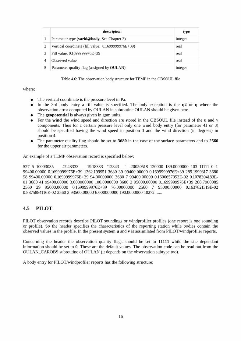
description type
1 Parameter type (varid@body, See Chapter 3) integer
2 Vertical coordinate (fill value: 0.1699999976E+39) real
3 Fill value: 0.1699999976E+39 real
4 Observed value real
5 Parameter quality flag (assigned by OULAN) integer
Table 4.6: The observation body structure for TEMP in the OBSOUL file
where:
● The vertical coordinate is the pressure level in Pa. ● In the 3rd body entry a fill value is specified. The only exception is the q2 or q where the
observation error computed by OULAN in subroutine OULAN should be given here. ● The geopotential is always given in gpm units. ● For the wind the wind speed and direction are stored in the OBSOUL file instead of the u and v
components. Thus for a certain pressure level only one wind body entry (for parameter 41 or 3) should be specified having the wind speed in position 3 and the wind direction (in degrees) in position 4.
● The parameter quality flag should be set to 3680 in the case of the surface parameters and to 2560 for the upper air parameters.
An example of a TEMP observation record is specified below:
527 5 10003035 47.43333 19.18333 '12843 ' 20050518 120000 139.0000000 103 11111 0 1 99400.00000 0.1699999976E+39 1362.199951 3680 39 99400.00000 0.1699999976E+39 289.1999817 3680 58 99400.00000 0.1699999976E+39 94.00000000 3680 7 99400.00000 0.1606657053E-02 0.1078304183E-01 3680 41 99400.00000 3.000000000 100.0000000 3680 2 95000.00000 0.1699999976E+39 288.7900085 2560 29 95000.00000 0.1699999976E+39 76.00000000 2560 7 95000.00000 0.1637821319E-02 0.8875884116E-02 2560 3 93500.00000 6.000000000 190.0000000 10272 .....
4.5 PILOT
PILOT observation records describe PILOT soundings or windprofiler profiles (one report is one sounding or profile). So the header specifies the characteristics of the reporting station while bodies contain the observed values in the profile. In the present system u and v is assimilated from PILOT/windprofiler reports.
Concerning the header the observation quality flags should be set to 11111 while the site dependant information should be set to 0. These are the default values. The observation code can be read out from the OULAN_CAROBS subroutine of OULAN (it depends on the observation subtype too).
A body entry for PILOT/windprofiler reports has the following structure:
16

description type
1 Parameter type (varid@body, See Chapter 3) integer
2 Vertical coordinate (fill value: 0.1699999976E+39) real
3 Fill value: 0.1699999976E+39 real
4 Observed value real
5 Parameter quality flag (assigned by OULAN) integer
Table 4.7: The observation body structure for PILOT in the OBSOUL file
● The vertical coordinate is the height of the observations in m. ● For the wind the wind speed and direction are stored in the OBSOUL file instead of the u and v
components. Thus for a certain pressure level only one wind body entry (for parameter 3) should be specified having the wind speed in position 3 and the wind direction (in degrees) in position 4.
● The parameter quality flag should be set to 4111.
An example of a windprofiler observation record is specified below:
72 6 10015134 48.10000 16.60000 'VIEWP ' 20050518 120500 227.0000000 12 11111 0 3 285.0000000 4.400000095 297.0000000 4111 3 328.0000000 8.800000191 310.0000000 4111 3 372.0000000 4.500000000 292.0000000 4111 3 415.0000000 7.099999905 319.0000000 4111 3 632.0000000 7.900000095 330.0000000 4111 3 675.0000000 6.199999809 336.0000000 4111 3 718.0000000 5.500000000 325.0000000 4111 3 762.0000000 3.500000000 318.0000000 4111 3 805.0000000 4.300000191 302.0000000 4111 3 502.0000000 9.100000381 313.0000000 4111 3 791.0000000 3.400000095 325.0000000 4111 3 1080.000000 1.100000024 165.0000000 4111
4.6 SATEM
A SATEM observation record/report describes one pixel for all the channels of a satellite sensor. The header specifies the characteristics of the report (location, time and satellite ID) while bodies contain the sensor ID, scanning parameters and the observed values. In the present system tbraw is assimilated from SATEM reports.
Concerning the header the observation quality flags should be set to 11111 while the site dependant information should be set to 0. These are the default values. The observation code can be read out from the OULAN_CAROBS_new subroutine of OULAN (it depends on the observation subtype too).
The first body entry for SATEM always contains information about the satellite sensor. It has the following structure:
description type
1 200 integer
2 Sensor ID (sensor@hdr) integer
3 Scan line real
4 Scan angle real
5 Fill value: 999999 integer
Table 4.8: The observation body structure for SATEM in the OBSOUL file. Part 1.
17
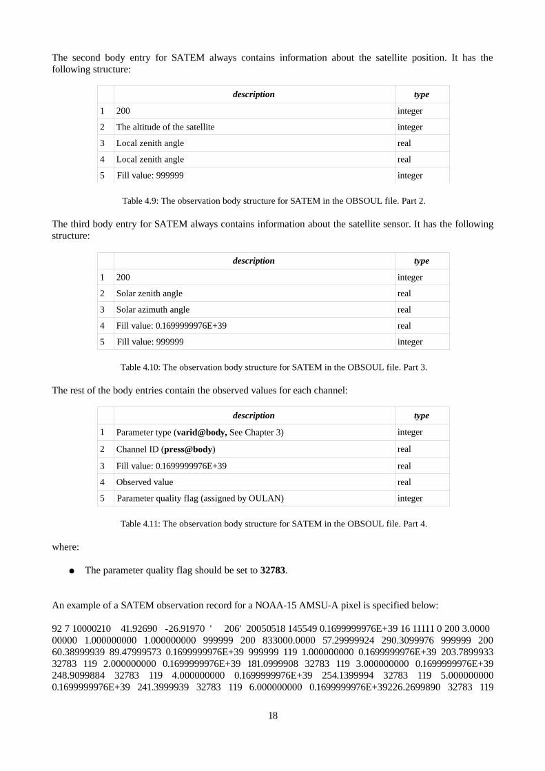
The second body entry for SATEM always contains information about the satellite position. It has the following structure:
description type
1 200 integer
2 The altitude of the satellite integer
3 Local zenith angle real
4 Local zenith angle real
5 Fill value: 999999 integer
Table 4.9: The observation body structure for SATEM in the OBSOUL file. Part 2.
The third body entry for SATEM always contains information about the satellite sensor. It has the following structure:
description type
1 200 integer
2 Solar zenith angle real
3 Solar azimuth angle real
4 Fill value: 0.1699999976E+39 real
5 Fill value: 999999 integer
Table 4.10: The observation body structure for SATEM in the OBSOUL file. Part 3.
The rest of the body entries contain the observed values for each channel:
description type
1 Parameter type (varid@body, See Chapter 3) integer
2 Channel ID (press@body) real
3 Fill value: 0.1699999976E+39 real
4 Observed value real
5 Parameter quality flag (assigned by OULAN) integer
Table 4.11: The observation body structure for SATEM in the OBSOUL file. Part 4.
where:
● The parameter quality flag should be set to 32783.
An example of a SATEM observation record for a NOAA-15 AMSU-A pixel is specified below:
92 7 10000210 41.92690 -26.91970 ' 206' 20050518 145549 0.1699999976E+39 16 11111 0 200 3.000000000 1.000000000 1.000000000 999999 200 833000.0000 57.29999924 290.3099976 999999 200 60.38999939 89.47999573 0.1699999976E+39 999999 119 1.000000000 0.1699999976E+39 203.7899933 32783 119 2.000000000 0.1699999976E+39 181.0999908 32783 119 3.000000000 0.1699999976E+39 248.9099884 32783 119 4.000000000 0.1699999976E+39 254.1399994 32783 119 5.000000000 0.1699999976E+39 241.3999939 32783 119 6.000000000 0.1699999976E+39226.2699890 32783 119
18

7.000000000 0.1699999976E+39 220.4299927 32783 119 8.000000000 0.1699999976E+39 216.5199890 32783 119 9.000000000 0.1699999976E+39 218.0499878 32783 119 10.00000000 0.1699999976E+39 221.8699951 32783 119 12.00000000 0.1699999976E+39 240.8399963 32783 119 13.00000000 0.1699999976E+39 254.959991532783 119 15.00000000 0.1699999976E+39 251.7299957 32783
19
5 Producing the OBSOUL file
The OBSOUL file can be produced in three different ways:
● with programme OULAN (the recommended way!)● with user-developed applications to put the observations into OBSOUL format● mixing the two solutions: using OULAN for some of the observation types and user-developed
applications for the other ones. In the end the resulting ASCII files can be simply concatenated together into the final OBSOUL file.
Please note that the OBSOUL file contains some specific codes that are properly set inside OULAN. So if someone wants to avoid the usage of OULAN then cannot avoid the study (or usage) of the code generating routines of OULAN. So that is an important reason why OULAN is recommended for OBSOUL generation!
5.1 Programme OULAN_hms
OULAN is developed by MF. The original version takes the observation data from the RDB database of MF. It is obvious therefore that this version of OULAN cannot be used outside MF. Thus, to use OULAN the observation reading part must be modified. At HMS Roger Randriamampianina made these modifications and developed the local version OULAN (OULAN_hms) that is now available from the LACE website (www.rclace.eu, in the Local Files menu).
5.1.1 The structure of OULAN_hms
The structure of OULAN_hms is rather simple. The main programme is oulan.f that only reads the namelists and calls subroutine OULAN_LAM_EXTRACT in oulan_lam_extract.f. This is the central routine that calls the different observation reading subroutines with the name EXT_LAM_obstype or EXT_obstype. These subroutines can be found in subroutine ext_lam_obstype.f in each case.
The other important routines are OULAN_CAROBS and OULAN_CAROBS_new (in oulan_carobs.f and oulan_carobs_new.f) which define special codes used in the OUBSOUL file (see Chapter 4 for details). The newer version of this subroutine is used to achieve the correct settings for GEOWIND and ATOVS/AMSU-B observations.
5.1.2 Observation usage in OULAN_hms
OULAN_hms can handle the following observations:
● SYNOP● TEMP● AIREP: AMDAR● SATOB: GEOWIND● PILOT: EUROPROFILER ● SATEM: ATOVS/AMSU-A, ATOVS/AMSU-B/MHS and ATOVS/HIRS
Some of the observations are not read directly in OULAN_hms. Instead an intermediate reader/converter is used to prepare an ASCII file which serves as input for OULAN_hms. To obtain these reader/converter applications please contact to Gergely Bölöni or Roger Randriamampianina. The available observation formats are as follows:
20

SYNOPSYNOP is stored in netCDF format at HMS. A new subroutine was added to OULAN_hms to read directly the netCDF files: ext_synop_netcdf.f. For other sites to use their own local SYNOP format only the local version of ext_synop_netcdf.f should be developed and the EXT_SYNOP_NETCDF subroutine call should be changed in ext_lam_synop.f.
AMDARAMDAR observations are available via the GTS in ASCII and BUFR formats. At HMS there is a dedicated script to convert these files into one ASCII file using a BUFR decoding software from the UK MetOffice. This ASCII file is then read directly by OULAN_hms. To obtain the converter application please contact to Gergely or Roger.
GEOWINDGEOWIND observations can be received via the EUMETCAST system in BUFR format. At HMS there is a dedicated script to convert these BUFR files into ASCII using the ECMWF BUFR decoding software. This ASCII file is then read directly by OULAN_hms. To obtain the converter application please contact to Roger.
TEMPTEMP is stored in netCDF format at HMS. A new subroutine was added to OULAN_hms to read directly the netCDF files: ext_temp_netcdf.f. For other sites to use their own local TEMP format only the local version of ext_temp_netcdf.f should be developed and the EXT_TEMP_NETCDF subroutine call should be changed in ext_temp_synop.f.
EUROPROFILERWindprofiler observations can be received via the GTS in BUFR format. At HMS there is a dedicated script to convert these BUFR files into ASCII using the ECMWF BUFR decoding software. This ASCII file is then read directly by OULAN_hms. To obtain the converter application please contact to Roger.
ATOVSOULAN_hms reads ATOVS data stored in the so-called "native format", which is the format of the output of the AAPP (AVHRR and ATOVS Preprocessing Package) package. At present ATOVS data is distributed in BUFR format through the EUMETCAST system. At HMS the converter from BUFR to native format is running on a little-endian (Linux) system that raises an endianess problem since OULAN is running on a big-endian systems. To handle this problem an endian converter is used when reading the ATOVS (AMSU-A, AMSUB/MHS and HIRS) data. To distinguish the big- and little-endian data a naming convention is used adding a suffix “swp” to the file name (see below) for the little-endian files. So the latest version of the OULAN_hms is handling both little- and big-endian ATOVS files. Respecting the naming convention, one can read at the same time both little- and big-endian files.
5.1.3 Running OULAN_hms
OULAN_hms is running on one processor. As an input it takes a namelist (under the name fort.4) and the observation files under the following names:
● SYNOP: synop● AMDAR: amdar_ascii.dat● GEOWIND: geowind_ascii.dat● TEMP: temp● EUROPROFILER: profiler_ascii.dat● ATOVS:
for files derived from AAPP conversion on big-endian systems:amsua01, amsua02, ...amsub01, amsub02, ...
21
hirs01, hirs02, .....for files derived from AAPP conversion on little-endian systems:
amsuaswp01, amsuaswp02, ...amsubswp01, amsubswp02, ...hirsswp01, hirsswp02, .....
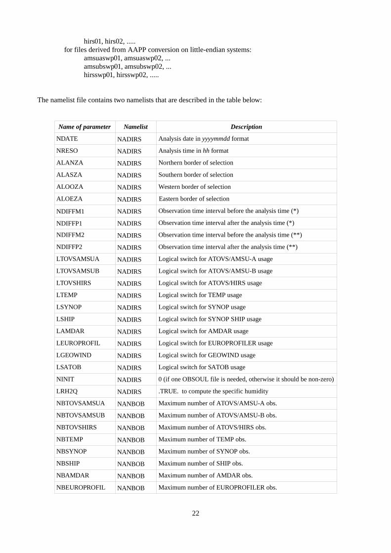
The namelist file contains two namelists that are described in the table below:
Name of parameter Namelist Description
NDATE NADIRS Analysis date in yyyymmdd format
NRESO NADIRS Analysis time in hh format
ALANZA NADIRS Northern border of selection
ALASZA NADIRS Southern border of selection
ALOOZA NADIRS Western border of selection
ALOEZA NADIRS Eastern border of selection
NDIFFM1 NADIRS Observation time interval before the analysis time (*)
NDIFFP1 NADIRS Observation time interval after the analysis time (*)
NDIFFM2 NADIRS Observation time interval before the analysis time (**)
NDIFFP2 NADIRS Observation time interval after the analysis time (**)
LTOVSAMSUA NADIRS Logical switch for ATOVS/AMSU-A usage
LTOVSAMSUB NADIRS Logical switch for ATOVS/AMSU-B usage
LTOVSHIRS NADIRS Logical switch for ATOVS/HIRS usage
LTEMP NADIRS Logical switch for TEMP usage
LSYNOP NADIRS Logical switch for SYNOP usage
LSHIP NADIRS Logical switch for SYNOP SHIP usage
LAMDAR NADIRS Logical switch for AMDAR usage
LEUROPROFIL NADIRS Logical switch for EUROPROFILER usage
LGEOWIND NADIRS Logical switch for GEOWIND usage
LSATOB NADIRS Logical switch for SATOB usage
NINIT NADIRS 0 (if one OBSOUL file is needed, otherwise it should be non-zero)
LRH2Q NADIRS .TRUE. to compute the specific humidity
NBTOVSAMSUA NANBOB Maximum number of ATOVS/AMSU-A obs.
NBTOVSAMSUB NANBOB Maximum number of ATOVS/AMSU-B obs.
NBTOVSHIRS NANBOB Maximum number of ATOVS/HIRS obs.
NBTEMP NANBOB Maximum number of TEMP obs.
NBSYNOP NANBOB Maximum number of SYNOP obs.
NBSHIP NANBOB Maximum number of SHIP obs.
NBAMDAR NANBOB Maximum number of AMDAR obs.
NBEUROPROFIL NANBOB Maximum number of EUROPROFILER obs.
22
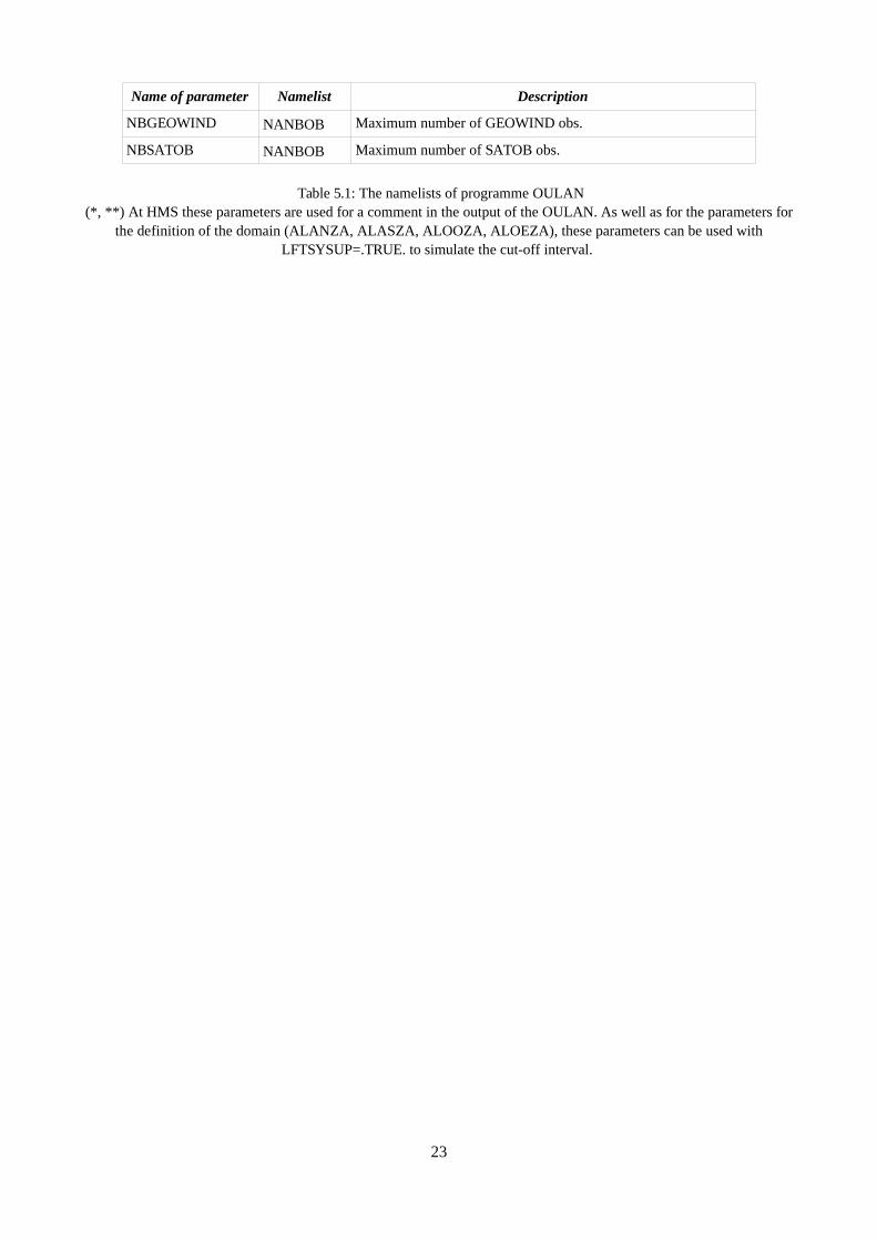
Name of parameter Namelist Description
NBGEOWIND NANBOB Maximum number of GEOWIND obs.
NBSATOB NANBOB Maximum number of SATOB obs.
Table 5.1: The namelists of programme OULAN(*, **) At HMS these parameters are used for a comment in the output of the OULAN. As well as for the parameters for
the definition of the domain (ALANZA, ALASZA, ALOOZA, ALOEZA), these parameters can be used with LFTSYSUP=.TRUE. to simulate the cut-off interval.
23

6 Programme BATOR
Programme BATOR is developed at MF and changing with the model cycles. It is available in the export packages under directory uti/bator. The main task of BATOR is the production of ECMA ODB sub-bases for data assimilation. Besides, the observation errors are also defined in BATOR. The third task of BATOR is the assignment of blacklisting information to the observations. A general documentation (in French) about BATOR is available on the web [4].
6.1 How to run BATOR
A BATOR run requires the following settings/inputs:
● setting of some environmental variables● file ficdate containing the time-slot definition ● file refdata describing the input files● file BATOR_MAP (not used at HMS)● file LISTE_NOIRE_DIAP (optional) for blacklisting ● file LISTE_LOC (optional) for blacklisting● observation inputs: it can be OBSOUL, BUFR or GRIB format● namelist for performing LAMFLAG filtering● namelist for reading the SEVIRI GRIB data
The environmental variables are as follows:
● ODB_CMA=ECMA● ODB_IO_METHOD =1 ● ODB_SRCPATH_ECMA = the location of the resulting ODB sub-bases' description files ● ODB_DATAPATH_ECMA = the location of the resulting ODB sub-bases' data files● BATOR_NBPOOL = The number of the pools in the resulting ODB sub-bases. The default is 1. ● BATOR_NBSLOT = The number of timeslots. For 3D-VAR it must be set to 1.● BATOR_LAMFLAG = 0/1. If it is 1 then the observation selection based on LAMFLAG is
activated. The default is 0. ● ODB_ANALYSIS_DATE = The date (yyyymmdd) of the analysis. ● ODB_ANALYSIS_TIME = The time (hh0000) of the analysis. ● BUFR_TABLES = The location of the BUFR tables.● TO_ODB_DEBUG = 0/1. If it is 1 detailed ODB related logging will be performed
BATOR will result in a set of ODB sub-bases with the name ECMA.base where the base suffix is specified in file refdata. These ODB sub-bases must be merged into a full ECMA ODB by programme SHUFFLE (for further details about it please read [6]).
6.2 Observation errors
The definition of the observation errors can be found in bator_init.F90. In this file the ECTERO array holds the observation error definition for all the parameters except the satellite radiances. The observation error will be assigned to the osb_error@errstat column of the resulting ODB.
24
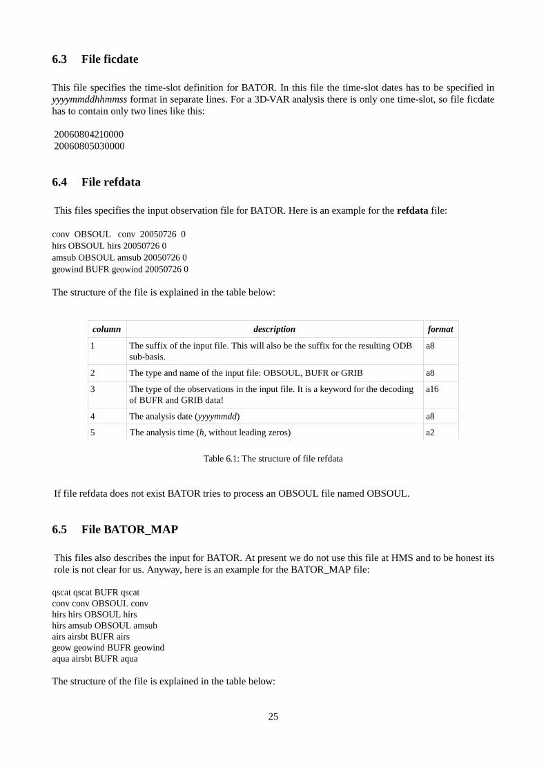
6.3 File ficdate
This file specifies the time-slot definition for BATOR. In this file the time-slot dates has to be specified in yyyymmddhhmmss format in separate lines. For a 3D-VAR analysis there is only one time-slot, so file ficdate has to contain only two lines like this:
2006080421000020060805030000
6.4 File refdata
This files specifies the input observation file for BATOR. Here is an example for the refdata file:
conv OBSOUL conv 20050726 0 hirs OBSOUL hirs 20050726 0amsub OBSOUL amsub 20050726 0geowind BUFR geowind 20050726 0
The structure of the file is explained in the table below:
column description format
1 The suffix of the input file. This will also be the suffix for the resulting ODB sub-basis.
a8
2 The type and name of the input file: OBSOUL, BUFR or GRIB a8
3 The type of the observations in the input file. It is a keyword for the decoding of BUFR and GRIB data!
a16
4 The analysis date (yyyymmdd) a8
5 The analysis time (h, without leading zeros) a2
Table 6.1: The structure of file refdata
If file refdata does not exist BATOR tries to process an OBSOUL file named OBSOUL.
6.5 File BATOR_MAP
This files also describes the input for BATOR. At present we do not use this file at HMS and to be honest its role is not clear for us. Anyway, here is an example for the BATOR_MAP file:
qscat qscat BUFR qscatconv conv OBSOUL convhirs hirs OBSOUL hirshirs amsub OBSOUL amsubairs airsbt BUFR airsgeow geowind BUFR geowindaqua airsbt BUFR aqua
The structure of the file is explained in the table below:
25
column description
1 Suffix for the ODB sub-base
2 Suffix for the input file
3 The type and name of the input file: OBSOUL, BUFR or GRIB
4 It is just a label
Table 6.2: The structure of file BATOR_MAP
6.6 Blacklisting
Blacklisting information is defined in two ASCII files: in LISTE_NOIRE_DIAP and LISTE LOC. As the result of blacklisting in the ODB the status.blacklist@body flags will be set to 1 for the blacklisted parameters.
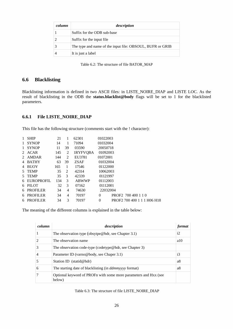
6.6.1 File LISTE_NOIRE_DIAP
This file has the following structure (comments start with the ! character):
1 SHIP 21 1 62301 010220031 SYNOP 14 1 71094 010320041 SYNOP 11 39 03590 200507182 ACAR 145 2 1RYFVQBA 010920032 AMDAR 144 2 EU3781 010720014 BATHY 63 39 ZSAF 010320044 BUOY 165 1 17546 011220005 TEMP 35 2 42314 100620035 TEMP 35 3 42339 011219976 EUROPROFIL 134 3 ABWWP 011120036 PILOT 32 3 07162 011120016 PROFILER 34 4 74630 220320046 PROFILER 34 4 70197 0 PROF2 700 400 1 1 0 6 PROFILER 34 3 70197 0 PROF2 700 400 1 1 1 H06 H18
The meaning of the different columns is explained in the table below:
column description format
1 The observation type (obsytpe@hdr, see Chapter 3.1) i2
2 The observation name a10
3 The observation code-type (codetype@hdr, see Chapter 3)
4 Parameter ID (varno@body, see Chaper 3.1) i3
5 Station ID (statid@hdr) a8
6 The starting date of blacklisting (in ddmmyyyy format) a8
7 Optional keyword of PROFn with some more parameters and Hxx (see below)
Table 6.3: The structure of file LISTE_NOIRE_DIAP
26

The blacklisting of certain parameters involves the automatic blacklisting of other parameters as well. These special cases are summarized in the table below:
obstype specified parameter blacklisted parameters
SYNOP 39 (t2) 39 (t2), 58 (rh2), 7 (q)
SYNOP 58 (rh2) 58 (rh2), 7 (q)
TEMP 1 (z) 1 (z), 29 (rh), 2 (t), 59 (td), 7 (q)
TEMP 2 (t) 2 (t), 29 (rh), 7 (q)
TEMP 29 (rh) 29 (rh), 7 (q)
Table 6.4: Special blacklisting in file LISTE_NOIRE_DIAP
There can be two kind of keywords in column 7 of LISTE_NOIRE_DIAP. The PROFn keyword makes possible the blacklisting of different pressure layers. It uses the following syntax:
PROFn P1 P2 .. Pn-1 I1 I2 ... In
where:● n can be at most 9 indicating the involved layers● the Pi values specify the bottom and top levels of pressure layers (in hPa). The first layer is always
[1000,P1[ ● and the Ii values indicate if blacklisting should be applied (=1) or not (=0) to the given layer.
The Hxx keyword specifies the analysis hour that should be blacklisted e.g. H00 or H06 etc. PROFn and Hxx keywords can be used together (like in the example above).
6.6.2 File LISTE_LOC
This file has the following structure (comments start with the ! character):
N 1 16N 2 141 29N 2 144 29N 2 145 29N 3 88 052N 3 88 054N 3 90 052 ZONB4 -50 50 13 113N 3 90 054 ZONB4 -50 50 -50 50N 3 88 253 ZONC4 -50 50 -155 105N 3 88 254 ZONC4 -50 50 -85 175N 3 88 256 ZONB4 -50 50 -125 -25N 6 34 4 PROF2 700 400 0 0 1N 6 134 3 PROF2 700 400 1 0 1N 7 210 206 3 TOVS2 6 11N 9 122 N 9 210 N 9 300
The meaning of the different columns is explained in the table below:
27

column description format
1 Type of action: N for blacklisted and O for forced to use a1
2 The observation type (obsytpe@hdr, see Chapter 3.1) i3
3 The observation code-type (codetype@hdr, see Chapter 3) i4
4 The satellite ID with leading zeros (satid@sat, see Chapter 3) a9
5 The centre that produced the satellite data i4
6 The parameter ID (varno@body, see Chaper 3.1) or the satellite sensor ID (sensor@hdr, see Chapter 3.7)
i4
7- Optional keywords of ZONx4, TOVSn, PPPPn, PROFn with some more parameters (see below)
Table 6.5: The structure of file LISTE_LOC
There can be four kind of keywords in column 7. The ZONx4 keyword can be applied to the SATOB/GEOWIND data using the following syntax:
ZONx4 latmin latmax lonmin lonmax
where:● if x=B then the pixels with lat < latmin or lat > latmax or lon < lonmin or lon >lonmax will be blacklisted● if x=C then the pixels with lat < latmin or lat > latmax or (lon > lonmin and lon < lonmax) will be
blacklisted.
The TOVSn keyword can be applied to ATOVS radiances using the following syntax:
TOVSn C1 C2 .... Cn
where:● n can be at most 9 indicating the involved channels● the Ci values specify the channels to be blacklisted .
The PPPPn keyword makes possible the blacklisting of different pressure levels. It uses the following syntax:
PPPPn P1 P2 ... Pn
where:● n can be at most 9 indicating the involved pressure levels● the Pi values specify the pressure levels (in hPa) to be blacklisted.
The PROFn keyword makes possible the blacklisting of different pressure layers. It uses the following syntax:
PROFn P1 P2 .. Pn-1 I1 I2 ... In
where:● n can be at most 9 indicating the involved layers● the Pi values specify the bottom and top levels of pressure layers (in hPa). The first layer is always
[1000,P1[ ● and the Ii values indicate if blacklisting should be applied (=1) or not (=0) to the given layer.
28

6.7 Observation files
As it was already explained BATOR can take three kinds of input files:
● The OBSOUL format and its generation process was presented in detail in Chapter 4 and 5. ● BATOR can also read BUFR files. At present GEOWIND observations, ATOVS AMSU/A and
AMSU/B radiances, AIRS radiances and QSCATT data can be provided in BUFR format to BATOR. Please note that BUFR usage in BATOR was never tested at HMS so more details can be added about this solution.
● BATOR reads SEVIRI data in GRIB format. The production of these GRIB files are presented in detail in [9].
6.8 LAMFLAG filtering
The main purpose of LAMFLAG filtering is to select only the observation inside the C+I domain. If this filtering is skipped the observation screening will abort. Formerly LAMFLAG was a separate application but from CY30 it has been integrated into BATOR. To invoke this filtering environmental variable BATOR_LAMFLAG has to set to 1 and a namelist has to be specified with the name of nam_LAMFLAG. The structure of this namelist is described in the table below:
Name of parameter Namelist Description
LOBSONLY NAMFCNT F/T if true, only select per obs type
ELAT0 NAMFGEOM degrees latitude of reference point of LAM domain
ELON NAMFGEOM degrees longitude of reference point of LAM domain
ELATC NAMFGEOM degrees latitude of centre point of LAM domain
ELONC NAMFGEOM degrees longitude of centre point of LAM domain
ELAT1 NAMFGEOM degrees latitude of SW corner of LAM domain
ELON1 NAMFGEOM degrees longitude of SW corner of LAM domain
EDELX NAMFGEOM meters x of the C+I grid
EDELY NAMFGEOM meters y of the C+I grid
NDLUN NAMFGEOM abscissa of first C+I point
NDGUN NAMFGEOM ordinate of first C+I point
NDLUX NAMFGEOM abscissa of last C+I point
NDGUX NAMFGEOM ordinate of last C+I poin
Z_CANZONE NAMFGEOM kilometers width for a wider selection (for CANARI)
REDZONE NAMFGEOM kilometers width for a tighter selection (reduce C+I)
REDZONE_N NAMFGEOM kilometers REDZONE only from the Northern border
REDZONE_S NAMFGEOM kilometers REDZONE only from the Southern border
REDZONE_W NAMFGEOM kilometers REDZONE only from the Western border
REDZONE_E NAMFGEOM kilometers REDZONE only from the Eastern border
LVAR NAMFGEOM T/F: selection will be done for 3dvar applications
LNEWGEOM NAMFGEOM T/F: origin of coordinate system will be SW cornerwhen false, and centre point when true
LSYNOP NAMFOBS T/F: false if SYNOP observations are to be skipped
29

Name of parameter Namelist Description
LAIREP NAMFOBS T/F: false if AIREP observations are to be skipped
LSATOB NAMFOBS T/F: false if SATOB observations are to be skipped
LDRIBU NAMFOBS T/F: false if DRIBU observations are to be skipped
LTEMP NAMFOBS T/F: false if TEMP observations are to be skipped
LPILOT NAMFOBS T/F: false if PILOT observations are to be skipped
LSATEM NAMFOBS T/F: false if SATEM observations are to be skipped
LPAOB NAMFOBS T/F: false if PAOB observations are to be skipped
LSCATT NAMFOBS T/F: false if scatterometer observations are to be skipped
LSLIMB NAMFOBS T/F: false if GPS observations are to be skipped
LRADAR NAMFOBS T/F: false if radar observations are to be skipped
Table 6.6: The structure of file namelist for LAMFLAG
30

7 Observation control in screening
The detailed description of screening is far beyond the goal of this document. Only some observation related issues are presented, mainly those that can be directly controlled by the users without any modifications in the source code. For more details about screening please study Chapter 10 in the IFS documentation [3], [2] and [10].
7.1 Screening decisions
Screening puts its quality control flags and decisions into the input ECMA ODB. Concerning the observation reports the following ODB columns are the most important (each is a bitfield type column):
● status@hdr: it contains the main quality control flags. The bits stored in status@hdr are as follows: active, passive, rejected and blacklisted.
● event1@hdr: it contains information about the reason of rejection and other events happened to the report during the screening
● blacklist@hdr: it contains information about the blacklisting.
As for the observed values, the following ODB columns are the most important (each is a bitfield type column):
● status@body: it contains the main quality control flags. The bits stored in status@body are as follows: active, passive, rejected and blacklisted. Only observations with status.active@body=1 can be used in the minimization!
● event1@body: it contains information about the reason of rejection and other events happened to the observation during the screening
● blacklist@body: it contains information about the blacklisting.
7.2 Blacklisting
In the screening various blacklisting techniques are applied. Most of them are hardcoded (in subroutines BLACKCLN and BLACKSAT) but a few of them can be controlled via namelist NAMOBS. These are as follows:
● A land-sea based rejection is applied to SYNOP, PILOT and TEMP reports controlled by the LSLREJ namelist variable. If this variable is .TRUE. (it is the default) then LSLRW10 (for wind 10m), LSLRT2 (for T2 m) and LSLRRH2 (for RHU 2m) controls the automatic rejection of the given observations over land.
● A height-based rejection is also applied controlled by the LHDLREJ namelist variable. If this variable is .TRUE. (it is the default) then LHDRW10 (for wind 10m), LHDRT2 (for T2 m) and LHDRRH2 (for RHU 2m) controls the height-based rejection of the given observation, i.e. if the difference between the model and the station elevation is too big then the rejection will be applied.
7.3 Background quality control
Data is rejected if the background departure is too big. In the background quality control, the square of the normalized background departure is considered as suspect when it exceeds its expected variance more than
31

by a predefined multiple (FGCHK). For the wind observations, the background quality control is performed simultaneously for both wind components (FGWND).
The procedure is as follows. It is known that the variance of the background departure for a given observation can be written as:
where σb is the taken from the errgrib file that contains grid-point background error values and interpolated into the observation location. This relation can be written into the following normalized form:
In practice, a background quality-control flag (rdbflag@body) is associated to the given observation that can be: 0 for a correct, 1 for a probably correct, 2 for a probably incorrect and 3 for an incorrect observation, respectively. This assignment is based on the following formula with the application of different Flaglimit values:
The predefined Flaglimit values for the background quality control in terms of multiples of the expected vari-ance of the normalized background departure. These values are set in DEFRUN and can be changed in namelist NAMJO.
For AIREP if the observed wind speed is less than 0.1 m/s and the background wind speed is larger than 5 m/s then the Flaglimit for the aircraft wind observation will be divided by 10. So this wind observation will be more likely to be rejected.
There is also a background quality control for the observed wind direction (FGWND). The predefined error limits of 60° , 90° and 120° apply for flag values 1, 2 and 3, respectively. The background quality control for the wind direction is applied only above 700 hPa for upper-air observations for wind speeds larger than 15 m/s. If the wind-direction background quality-control flag has been set to a value that is greater than or equal to 2, the background quality-control flag for the wind observations is increased by 1.
The background quality control rejection limits are flag value 3 for all the data, and flag value 2 for the non-standard-level data.
7.4 Thinning
A spatial thinning is performed in screening in order to avoid spatial correlations between observations. Thinning is applied for AIREP, satellite radiances and SATOB observations.
Concerning the thinning of AIREP data it is important to know that one AIREP flight consists of a set of reports. The thinning of AIREP observations is performed for each flight separately. During the thinning 3D boxes are constructed around model levels. In each box the report closest to the analysis date containing the largest number of active observations is selected. The box size is set in meters via the RMFIND_AIREP variable in the NAMSCC namelist.
32
y−H xb 2≈ b
2 o
2
y−H xb
b 2
≈1o
2
b2≡
y−H xb
b 2
Flaglimit×
For the satellite radiances a horizontal thinning is performed in two steps for each channel separately. In the first step a minimum distance is enforced between the pixels. This distance is defined in meters via the RMIND_RAD1C(sensor_id) variable in NAMSCC. Then a repeated thinning is performed to reach the final separation that is defined via RFIND_RAD1C(sensor_id) in NAMSCC. The sensor IDs are described in Chapter 3.7. In the pixel selection several criterion are taken into account: e.g. sea is preferred over land, clear sky pixel is preferred over a cloudy one etc.
The horizontal thinning of SATOB observations is similar to the satellite radiances: it is done in two steps controlled by RMIND_SATOB and RFIND_SATOB. Then a vertical thinning is performed using boxes around model levels. In each box the report closest to the analysis date containing the largest number of active observations is selected. The QI values are also used in the selection.
The thinning is performed in subroutines THINAIR and THINNER. The default values of the thinning distances are defined in module YOMSCC.
7.5 Satellite radiance bias correction
The satellite radiance bias correction is also performed in screening. It requires a set of coefficients stored in a certain ASCII file format. For details about the bias-correction method please read [8].
7.6 Output statistics
Screening provides detailed statistics about the observation usage and screening decisions. These statistics can be found in the NODE file of screening after the position of the “SCREENING STATISTICS” label.
33

8 Observation control in minimization
There is not much observation control in the minimization. Minimization takes a CCMA ODB and this ODB contains only observations that were regarded as active by screening. However, these observation will not be used directly by minimization but an additional setting is needed for it: in namelist NAMJO the NOTVAR arrays should be set carefully. The first index of NOTVAR is always 1 while the second index of NOTVAR refers the observation types (please see Chapter 3.1 for details). The order of elements of NOTVAR is defined in YOMCOSJO. If such an element is 0 then the given parameter will be used in the minimization.
For example, to use u10m (element 1), rh2m (element 6), Z (element 8) and t2m (element 11) for SYNOP reports NOTVAR(1,1) should be set as:
NOTVAR(1,1)= -1, 0,-1,-1,-1, 0,-1, 0,-1,-1, 0,-1,-1,-1,-1,-1,-1,-1,-1,-1,-1,-1,-1,-1,-1,
34
9 References
[1] Bölöni G., 2004: Technical note on observation handling in ALADIN CY28T0, available online at: http://www.rclace.eu /File/Data_Assimilation/2004/GB_T_N_obs_handling_AL_cy28t0_2004.ps
[2] Fischer C., L. Auger, B. Chapnik, 2007: The variational computations inside ARPEGE/ALADIN cycle CY32. Available online at: http://www.cnrm.meteo.fr/ gmapdoc/IMG/ps/main_var.ps
[3] IFS Documentation CY28R1, Part II: Data assimilation. Available online at: http://www.ecmwf.int/research/ifsdocs/CY28r1/pdf_files/Assimilation.pdf
[4] Puech D.: A web-based documentation about ODB in French available at the following address:http://www.cnrm.meteo.fr/gmapdoc/meshtml/DOC_odb/odb.html. In this page select link guide pratique to access the detailed information about the ODB tables and columns. The same document contains information about BATOR, as well.
[5] Randriamampianina R., 2006: Observation preprocessing in the ARPEGE/ALADIN model. Part 1: OULAN.
Available online at: http://www.rclace.eu/File/Data_Assimilation/workshops/Bp_workshop_OULAN.ppt
[6] Randriamampianina R., 2006: Observation preprocessing in the ARPEGE/ALADIN model. Part 2: BATOR. Available online at: http://www.rclace.eu/File/Data_Assimilation/workshops/Bp_workshop_BATOR.ppt
[7] Randriamampianina R., 2006: Observation preprocessing in the ARPEGE/ALADIN model. Part 3: 1C radiance bias-correction. Available online at:http://www.rclace.eu/File/Data_Assimilation/workshops/Bp_workshop_BiasCorr.ppt
[8] Saarinen S., 2004: ODB User Guide. This detailed introduction to ODB is available at the following address: http://www.ecmwf.int/research/ifsdocs/CY28r1/pdf_files/odb.pdf
[9] Trojakova A. 2006: Assimilation of SEVIRI data. Available online at:http://www.rclace.eu/File/Data_Assimilation/2006/AT_MM_LACE_report_SEVIRI_2006.pdf
[10] ALADIN 3D-VAR and ODB training, 6-10 June, 2006, HMS, Budapest. Training materials available online at: http://www.rclace.eu under the Research Areas -> Data Assimilation menu.
10 Acknowledgements
The expertise and work of my colleagues at HMS, specially that of Roger Randriamampianina, is strongly supported me in the preparation of this document.
35