
Overview Constraint Programming - unibo.it · Essentials of Constraint Programming, Thom...
101
Constraint Programming Constraint Programming Prof. Dr. Thom Fr ¨ uhwirth February 8, 2006 slides by Marc Meister Based on: Essentials of Constraint Programming, Thom Fr ¨ uhwirth and Slim Abdennadher, Textbook, Springer Verlag, 2003. Thom Fr ¨ uhwirth – University of Ulm Page 1 – WS 2005 Constraint Programming Overview • Introduction • Foundation from Logics • Constraint Languages – Syntax – Declarative and Operational Semantics – Soundness and Completeness • Constraint Systems – Constraint Theory – Solving Algorithms – Applications Thom Fr ¨ uhwirth – University of Ulm Page 2 – WS 2005 Constraint Programming The Holy Grail Constraint Programming represents one of the closest approaches computer science has yet made to the Holy Grail of programming: the user states the problem, the computer solves it. Eugene C. Freuder, Inaugural issue of the Constraints Journal, 1997. Thom Fr ¨ uhwirth – University of Ulm Page 3 – WS 2005 Constraint Programming Constraint Reasoning The Idea • Example – Combination Lock: 0 1 2 3 4 5 6 7 8 9 Greater or equal 5. Prime number. • Declarative problem representation by variables and constraints: x ∈{0, 1,..., 9}∧ x ≥ 5 ∧ prime(x) • Constraint propagation and simplification reduce search space: x ∈{0, 1,..., 9}∧ x ≥ 5 → x ∈{5, 6, 7, 8, 9} Thom Fr ¨ uhwirth – University of Ulm Page 4 – WS 2005
Transcript of Overview Constraint Programming - unibo.it · Essentials of Constraint Programming, Thom...
Constraint Programming
Constraint Programming
Prof. Dr. Thom Fruhwirth
February 8, 2006
slides by Marc Meister
Based on:
Essentials of Constraint Programming,
Thom Fruhwirth and Slim Abdennadher,
Textbook, Springer Verlag, 2003.
Thom Fruhwirth – University of Ulm Page 1 – WS 2005
Constraint Programming
Overview
• Introduction
• Foundation from Logics
• Constraint Languages
– Syntax
– Declarative and Operational Semantics
– Soundness and Completeness
• Constraint Systems
– Constraint Theory
– Solving Algorithms
– Applications
Thom Fruhwirth – University of Ulm Page 2 – WS 2005
Constraint Programming
The Holy Grail
Constraint Programming represents one of the closest
approaches computer science has yet made to the Holy Grail
of programming: the user states the problem, the computer
solves it.
Eugene C. Freuder, Inaugural issue of the Constraints Journal, 1997.
Thom Fruhwirth – University of Ulm Page 3 – WS 2005
Constraint Programming
Constraint Reasoning
The Idea
• Example – Combination Lock:
0 1 2 3 4 5 6 7 8 9
Greater or equal 5.
Prime number.
• Declarative problem representation by variables and constraints:
x ∈ {0, 1, . . . , 9} ∧ x ≥ 5 ∧ prime(x)
• Constraint propagation and simplification reduce search space:
x ∈ {0, 1, . . . , 9} ∧ x ≥ 5 → x ∈ {5, 6, 7, 8, 9}
Thom Fruhwirth – University of Ulm Page 4 – WS 2005
Constraint Programming
Constraint Programming
Robust, flexible, maintainable software faster.
• Declarative modeling by constraints:
Description of properties and relationships between partially
known objects.
Correct handling of precise and imprecise, finite and infinite,
partial and full information.
• Automatic constraint reasoning:
Propagation of the effects of new information (as constraints).
Simplification makes implicit information explicit.
• Solving combinatorial problems efficiently:
Easy Combination of constraint solving with search and
optimization.
Thom Fruhwirth – University of Ulm Page 5 – WS 2005
Constraint Programming
Terminology
Language is first-order logic with equality.
• Constraint:
Conjunction of atomic constraints (predicates)
E.g., 4X + 3Y = 10 ∧ 2X − Y = 0
• Constraint Problem (Query):
A given, initial constraint
• Constraint Solution (Answer):
A valuation for the variables in a given constraint problem that
satisfies all constraints of the problem. E.g., X = 1 ∧ Y = 2
In general, a normal/solved form of, e.g., the problem
4X + 3Y + Z = 10 ∧ 2X − Y = 0 simplifies into
Y + Z = 10 ∧ 2X − Y = 0
Thom Fruhwirth – University of Ulm Page 6 – WS 2005
Constraint Programming
Constraint Reasoning and Constraint Programming
A generic framework for
• Modeling
– with partial information
– with infinite information
• Reasoning
– with new information
• Solving
– combinatorial problems
Thom Fruhwirth – University of Ulm Page 7 – WS 2005
Constraint Programming
Constraint Programming – Mortgage
% D: Amount of Loan, Debt, Principal
% T: Duration of loan in months
% I: Interest rate per month
% R: Rate of payments per month
% S: Balance of debt after T months
mortgage(D, T, I, R, S) <=>
T = 0,
D = S
;
T > 0,
T1 = T - 1,
D1 = D + D*I - R,
mortgage(D1, T1, I, R, S).
Thom Fruhwirth – University of Ulm Page 8 – WS 2005
Constraint Programming
Constraint Programming – Mortgage (cont)
• mortgage(100000,360,0.01,1025,S) yields S=12625.90.
• mortgage(D,360,0.01,1025,0) yields D=99648.79.
• S=<0, mortgage(100000,T,0.01,1025,S)
yields T=374, S=-807.96.
• mortgage(D,360,0.01,R,0) yields R=0.0102861198*D.
• If the interest rate I is unknown, the equation D1 = D + D*I -
R will be non-linear after one recursion step, since D1, the new D,
is not determined either.
Thom Fruhwirth – University of Ulm Page 9 – WS 2005
Constraint Programming
Aspects of Constraint Logic Programming
Theoretical
Logical Foundation – First-Order Logic
Conceptual
Sound Modeling
Practical
Efficient Algorithms/Implementations
Combination of different Solvers
Thom Fruhwirth – University of Ulm Page 10 – WS 2005
Constraint Programming
Constraint Solving
Adaption and combination of existing efficient algorithms from
• Mathematics
– Operations research
– Graph theory
– Algebra
• Computer science
– Finite automata
– Automatic proving
• Economics
• Linguistics
Thom Fruhwirth – University of Ulm Page 11 – WS 2005
Constraint Programming
Early History of Constraint Programming
60s, 70s Constraint networks in artificial intelligence.
70s Logic programming (Prolog).
80s Constraint logic programming.
80s Concurrent logic programming.
90s Concurrent constraint programming.
90s Commercial applications.
Thom Fruhwirth – University of Ulm Page 12 – WS 2005
Constraint Programming
Application Domains
• Modeling
• Executable Specifications
• Solving combinatorial problems
– Scheduling, Planning, Timetabling
– Configuration, Layout, Placement, Design
– Analysis: Simulation, Verification, Diagnosis
of software, hardware and industrial processes.
Thom Fruhwirth – University of Ulm Page 13 – WS 2005
Constraint Programming
Application Domains (cont)
• Artificial Intelligence
– Machine Vision
– Natural Language Understanding
– Temporal and Spatial Reasoning
– Theorem Proving
– Qualitative Reasoning
– Robotics
– Agents
– Bio-informatics
Thom Fruhwirth – University of Ulm Page 14 – WS 2005
Constraint Programming
Applications in Research
• Computer Science: Program Analysis, Robotics, Agents
• Molecular Biology, Biochemistry, Bio-informatics:
Protein Folding, Genomic Sequencing
• Economics: Scheduling
• Linguistics: Parsing
• Medicine: Diagnosis Support
• Physics: System Modeling
• Geography: Geo-Information-Systems
Thom Fruhwirth – University of Ulm Page 15 – WS 2005
Constraint Programming
Early Commercial Applications
• Lufthansa: Short-term staff planning.
• Hong Kong Container Harbor: Resource planning.
• Renault: Short-term production planning.
• Nokia: Software configuration for mobile phones.
• Airbus: Cabin layout.
• Siemens: Circuit verification.
• Caisse d’epargne: Portfolio management.
In Decision Support Systems for Planning, Configuration, for Design,
Analysis.
Thom Fruhwirth – University of Ulm Page 16 – WS 2005
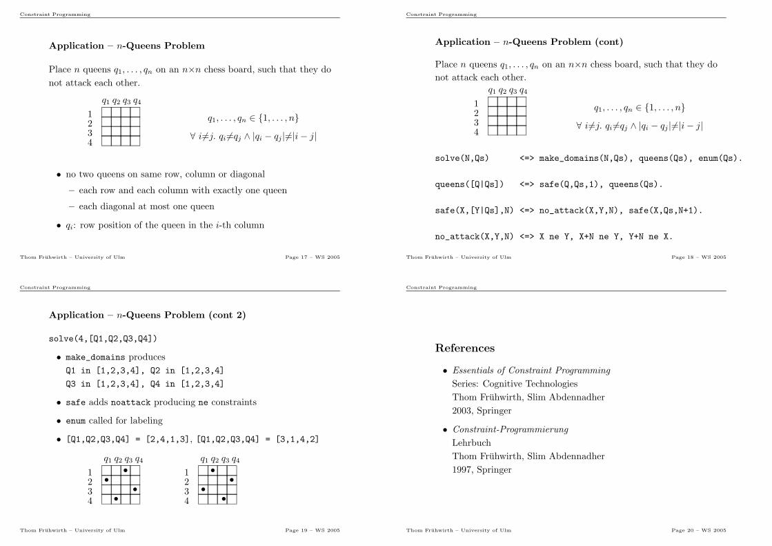
Constraint Programming
Application – n-Queens Problem
Place n queens q1, . . . , qn on an n×n chess board, such that they do
not attack each other.
1234
q1 q2 q3 q4
q1, . . . , qn ∈ {1, . . . , n}∀ i6=j. qi 6=qj ∧ |qi − qj |6=|i− j|
• no two queens on same row, column or diagonal
– each row and each column with exactly one queen
– each diagonal at most one queen
• qi: row position of the queen in the i-th column
Thom Fruhwirth – University of Ulm Page 17 – WS 2005
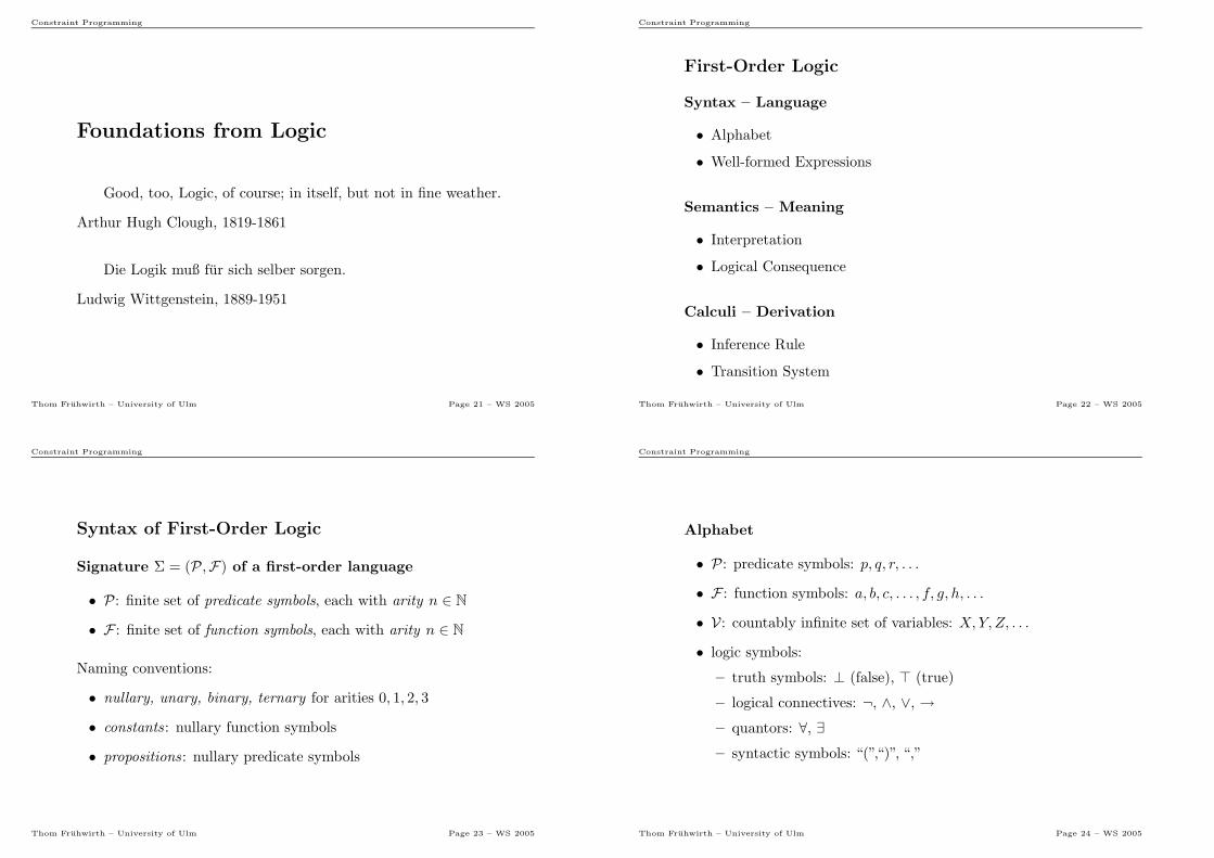
Constraint Programming
Application – n-Queens Problem (cont)
Place n queens q1, . . . , qn on an n×n chess board, such that they do
not attack each other.
1234
q1 q2 q3 q4
q1, . . . , qn ∈ {1, . . . , n}∀ i6=j. qi 6=qj ∧ |qi − qj |6=|i− j|
solve(N,Qs) <=> make_domains(N,Qs), queens(Qs), enum(Qs).
queens([Q|Qs]) <=> safe(Q,Qs,1), queens(Qs).
safe(X,[Y|Qs],N) <=> no_attack(X,Y,N), safe(X,Qs,N+1).
no_attack(X,Y,N) <=> X ne Y, X+N ne Y, Y+N ne X.
Thom Fruhwirth – University of Ulm Page 18 – WS 2005
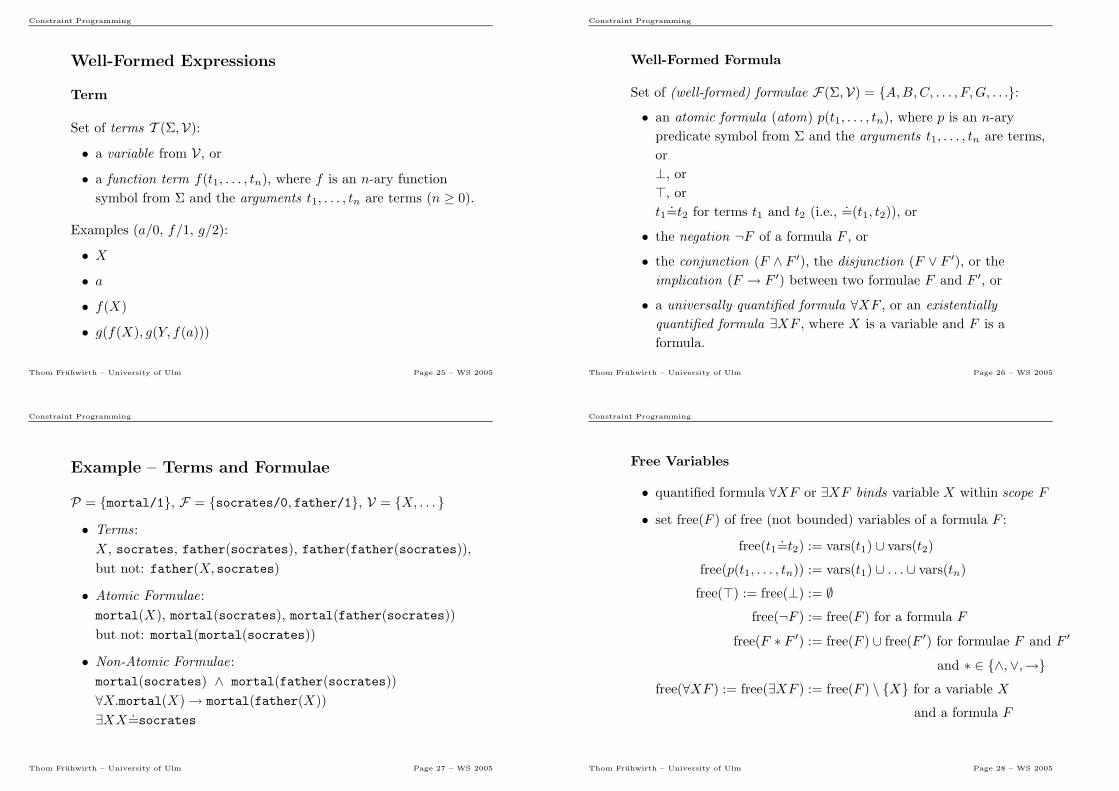
Constraint Programming
Application – n-Queens Problem (cont 2)
solve(4,[Q1,Q2,Q3,Q4])
• make_domains produces
Q1 in [1,2,3,4], Q2 in [1,2,3,4]
Q3 in [1,2,3,4], Q4 in [1,2,3,4]
• safe adds noattack producing ne constraints
• enum called for labeling
• [Q1,Q2,Q3,Q4] = [2,4,1,3], [Q1,Q2,Q3,Q4] = [3,1,4,2]
1234
••
••
q1 q2 q3 q4
1234
••
••
q1 q2 q3 q4
Thom Fruhwirth – University of Ulm Page 19 – WS 2005
Constraint Programming
References
• Essentials of Constraint Programming
Series: Cognitive Technologies
Thom Fruhwirth, Slim Abdennadher
2003, Springer
• Constraint-Programmierung
Lehrbuch
Thom Fruhwirth, Slim Abdennadher
1997, Springer
Thom Fruhwirth – University of Ulm Page 20 – WS 2005
Constraint Programming
Foundations from Logic
Good, too, Logic, of course; in itself, but not in fine weather.
Arthur Hugh Clough, 1819-1861
Die Logik muß fur sich selber sorgen.
Ludwig Wittgenstein, 1889-1951
Thom Fruhwirth – University of Ulm Page 21 – WS 2005
Constraint Programming
First-Order Logic
Syntax – Language
• Alphabet
• Well-formed Expressions
Semantics – Meaning
• Interpretation
• Logical Consequence
Calculi – Derivation
• Inference Rule
• Transition System
Thom Fruhwirth – University of Ulm Page 22 – WS 2005
Constraint Programming
Syntax of First-Order Logic
Signature Σ = (P,F) of a first-order language
• P: finite set of predicate symbols, each with arity n ∈ N
• F : finite set of function symbols, each with arity n ∈ N
Naming conventions:
• nullary, unary, binary, ternary for arities 0, 1, 2, 3
• constants: nullary function symbols
• propositions: nullary predicate symbols
Thom Fruhwirth – University of Ulm Page 23 – WS 2005
Constraint Programming
Alphabet
• P: predicate symbols: p, q, r, . . .
• F : function symbols: a, b, c, . . . , f, g, h, . . .
• V : countably infinite set of variables: X,Y, Z, . . .
• logic symbols:
– truth symbols: ⊥ (false), ⊤ (true)
– logical connectives: ¬, ∧, ∨, →– quantors: ∀, ∃– syntactic symbols: “(”,“)”, “,”
Thom Fruhwirth – University of Ulm Page 24 – WS 2005
Constraint Programming
Well-Formed Expressions
Term
Set of terms T (Σ,V):
• a variable from V , or
• a function term f(t1, . . . , tn), where f is an n-ary function
symbol from Σ and the arguments t1, . . . , tn are terms (n ≥ 0).
Examples (a/0, f/1, g/2):
• X• a• f(X)
• g(f(X), g(Y, f(a)))
Thom Fruhwirth – University of Ulm Page 25 – WS 2005
Constraint Programming
Well-Formed Formula
Set of (well-formed) formulae F(Σ,V) = {A,B,C, . . . , F,G, . . .}:• an atomic formula (atom) p(t1, . . . , tn), where p is an n-ary
predicate symbol from Σ and the arguments t1, . . . , tn are terms,
or
⊥, or
⊤, or
t1=t2 for terms t1 and t2 (i.e., =(t1, t2)), or
• the negation ¬F of a formula F , or
• the conjunction (F ∧ F ′), the disjunction (F ∨ F ′), or the
implication (F → F ′) between two formulae F and F ′, or
• a universally quantified formula ∀XF , or an existentially
quantified formula ∃XF , where X is a variable and F is a
formula.
Thom Fruhwirth – University of Ulm Page 26 – WS 2005
Constraint Programming
Example – Terms and Formulae
P = {mortal/1}, F = {socrates/0, father/1}, V = {X, . . . }
• Terms:
X , socrates, father(socrates), father(father(socrates)),
but not: father(X, socrates)
• Atomic Formulae:
mortal(X), mortal(socrates), mortal(father(socrates))
but not: mortal(mortal(socrates))
• Non-Atomic Formulae:
mortal(socrates) ∧ mortal(father(socrates))
∀X.mortal(X)→ mortal(father(X))
∃XX=socrates
Thom Fruhwirth – University of Ulm Page 27 – WS 2005
Constraint Programming
Free Variables
• quantified formula ∀XF or ∃XF binds variable X within scope F
• set free(F ) of free (not bounded) variables of a formula F :
free(t1=t2) := vars(t1) ∪ vars(t2)
free(p(t1, . . . , tn)) := vars(t1) ∪ . . . ∪ vars(tn)
free(⊤) := free(⊥) := ∅free(¬F ) := free(F ) for a formula F
free(F ∗ F ′) := free(F ) ∪ free(F ′) for formulae F and F ′
and ∗ ∈ {∧,∨,→}free(∀XF ) := free(∃XF ) := free(F ) \ {X} for a variable X
and a formula F
Thom Fruhwirth – University of Ulm Page 28 – WS 2005
Constraint Programming
Example – Free Variables
Give the set of free variables for each braced part.
p(X) ∧︷ ︸︸ ︷
∃Xp(X)︸ ︷︷ ︸
︷ ︸︸ ︷(∀X p(X,Y )
︸ ︷︷ ︸
)
︸ ︷︷ ︸
∨ q(X)︸ ︷︷ ︸
Thom Fruhwirth – University of Ulm Page 29 – WS 2005
Constraint Programming
Universal and Existential Closure of F
• universal closure ∀F of F :
∀X1∀X2 . . .∀XnF
• existential closure ∃F of F :
∃X1∃X2 . . .∃XnF
where X1, X2, . . . , Xn are all free variables of F
Naming Conventions:
• closed formula or sentence: does not contain free variables
• theory : set of sentences
• ground term or formula: does not contain any variables
Thom Fruhwirth – University of Ulm Page 30 – WS 2005
Constraint Programming
Semantics of First-Order Logic
Interpretation I of Σ
• universe U : a non-empty set
• I(f) : Un → U : a function for every n-ary function symbol f of Σ
• I(p) ⊆ Un: a relation for every n-ary predicate symbol p of Σ
Variable Valuation for V w.r.t. I
• η : V → U : for every variable X of V into the universe U of I
(Σ signature of a first-order language, V set of variables)
Thom Fruhwirth – University of Ulm Page 31 – WS 2005
Constraint Programming
Interpretation of Terms
ηI : T (Σ, V )→ U : for every term
ηI(X) := η(X) for a variable X
ηI(f(t1, . . . , tn)) := I(f)(ηI(t1), . . . , ηI(tn))
for an n-ary function symbol f and terms t1, . . . , tn
(Σ signature, I interpretation with universe U , η : V → U variable
valuation)
Thom Fruhwirth – University of Ulm Page 32 – WS 2005
Constraint Programming
Example – Interpretation of Terms
• signature Σ = (∅, {1/0, */2, +/2})• universe U = N
• interpretation I
I(1) := 1
I(A+B) := A+B, I(A*B) := AB for A,B ∈ U• variable valuation η
η(X) := 3, η(Y ) := 5
ηI(X*(Y +1)
)= I(*)
(ηI(X), ηI(Y +1)
)
= I(*)(3, I(+)(ηI(Y ), ηI(1)
)
= · · · = 3 · (5 + 1) = 18
Thom Fruhwirth – University of Ulm Page 33 – WS 2005
Constraint Programming
Interpretation of Formulae – Preliminaries
For a function g, the function g[Y 7→ a] is
g[Y 7→ a](X) :=
g(X) if X 6= Y,
a if X = Y,
where X and Y are variables.
Thom Fruhwirth – University of Ulm Page 34 – WS 2005
Constraint Programming
Interpretation of Formulae
I interpretation of Σ, η variable valuation satisfy F written I, η |= F :
• I, η |= ⊤ and I, η 6|= ⊥• I, η |= s=t iff ηI(s) = ηI(t)
• I, η |= p(t1, . . . , tn) iff (ηI(t1), . . . , ηI(tn)) ∈ I(p)
• I, η |= ¬F iff I, η 6|= F
• I, η |= F ∧ F ′ iff I, η |= F and I, η |= F ′
• I, η |= F ∨ F ′ iff I, η |= F or I, η |= F ′
• I, η |= F → F ′ iff I, η 6|= F or I, η |= F ′
• I, η |= ∀XF iff I, η[X 7→ u] |= F for all u ∈ U• I, η |= ∃XF iff I, η[X 7→ u] |= F for some u ∈ U
Thom Fruhwirth – University of Ulm Page 35 – WS 2005
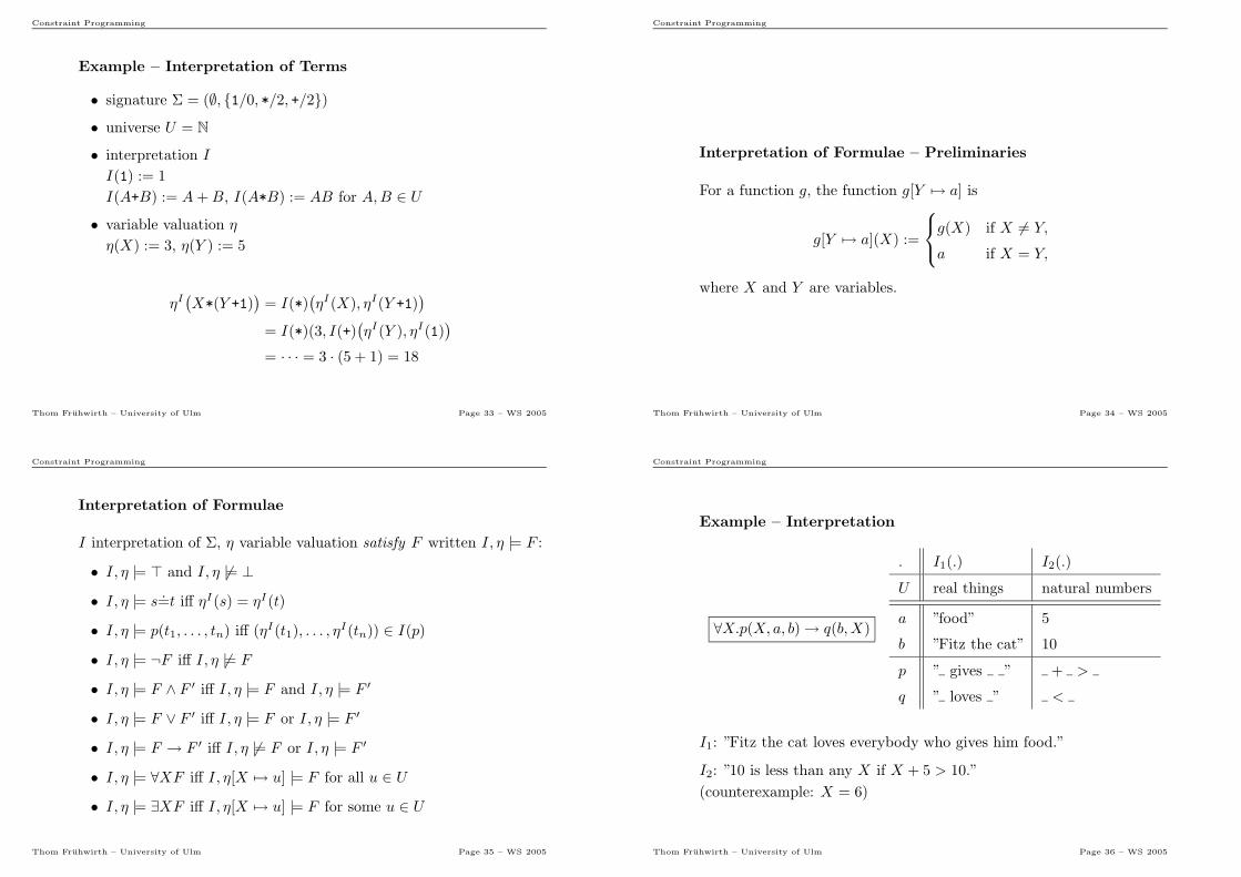
Constraint Programming
Example – Interpretation
∀X.p(X, a, b)→ q(b,X)
. I1(.) I2(.)
U real things natural numbers
a ”food” 5
b ”Fitz the cat” 10
p ” gives ” + >
q ” loves ” <
I1: ”Fitz the cat loves everybody who gives him food.”
I2: ”10 is less than any X if X + 5 > 10.”
(counterexample: X = 6)
Thom Fruhwirth – University of Ulm Page 36 – WS 2005
Constraint Programming
Model of F , Validity
• I model of F or I satisfies F , written I |= F :
I, η |= F for every variable valuation η
• I model of theory T : I model of each formula in T
Sentence S is
• valid : satisfied by every interpretation, i.e., I |= S for every I
• satisfiable: satisfied by some interpretation, i.e., I |= S for some I
• falsifiable: not satisfied by some interpretation, i.e., I 6|= S for
some I
• unsatisfiable: not satisfied by any interpretation, i.e., I 6|= S for
every I
(Σ signature, I interpretation)
Thom Fruhwirth – University of Ulm Page 37 – WS 2005
Constraint Programming
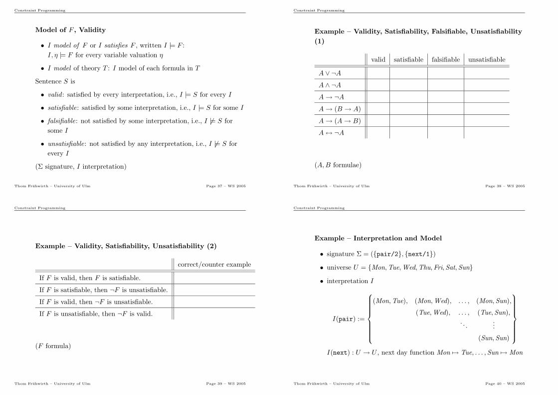
Example – Validity, Satisfiability, Falsifiable, Unsatisfiability
(1)
valid satisfiable falsifiable unsatisfiable
A ∨ ¬AA ∧ ¬AA→ ¬AA→ (B → A)
A→ (A→ B)
A↔ ¬A
(A,B formulae)
Thom Fruhwirth – University of Ulm Page 38 – WS 2005
Constraint Programming
Example – Validity, Satisfiability, Unsatisfiability (2)
correct/counter example
If F is valid, then F is satisfiable.
If F is satisfiable, then ¬F is unsatisfiable.
If F is valid, then ¬F is unsatisfiable.
If F is unsatisfiable, then ¬F is valid.
(F formula)
Thom Fruhwirth – University of Ulm Page 39 – WS 2005
Constraint Programming
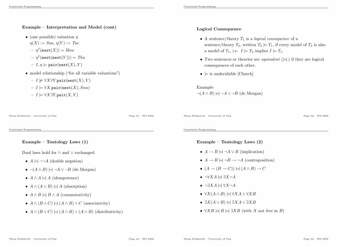
Example – Interpretation and Model
• signature Σ = ({pair/2}, {next/1})
• universe U = {Mon,Tue,Wed,Thu,Fri, Sat, Sun}
• interpretation I
I(pair) :=
(Mon,Tue), (Mon,Wed), . . . , (Mon, Sun),
(Tue,Wed), . . . , (Tue, Sun),
. . ....
(Sun, Sun)
I(next) : U → U , next day function Mon 7→ Tue, . . . ,Sun 7→ Mon
Thom Fruhwirth – University of Ulm Page 40 – WS 2005
Constraint Programming
Example – Interpretation and Model (cont)
• (one possible) valuation η
η(X) := Sun, η(Y ) := Tue
– ηI(next(X)) = Mon
– ηI(next(next(Y ))) = Thu
– I, η |= pair(next(X), Y )
• model relationship (“for all variable valuations”)
– I 6|= ∀X∀Y.pair(next(X), Y )
– I |= ∀X.pair(next(X), Sun)
– I |= ∀X∃Y.pair(X,Y )
Thom Fruhwirth – University of Ulm Page 41 – WS 2005
Constraint Programming
Logical Consequence
• A sentence/theory T1 is a logical consequence of a
sentence/theory T2, written T2 |= T1, if every model of T2 is also
a model of T1, i.e. I |= T2 implies I |= T1.
• Two sentences or theories are equivalent (|=| ) if they are logical
consequences of each other.
• |= is undecidable [Church]
Example:
¬(A ∧B) |=| ¬A ∨ ¬B (de Morgan)
Thom Fruhwirth – University of Ulm Page 42 – WS 2005
Constraint Programming
Example – Tautology Laws (1)
Dual laws hold for ∧ and ∨ exchanged.
• A |=| ¬¬A (double negation)
• ¬(A ∧B) |=| ¬A ∨ ¬B (de Morgan)
• A ∧A |=| A (idempotence)
• A ∧ (A ∨B) |=|A (absorption)
• A ∧B |=|B ∧A (commutativity)
• A ∧ (B ∧ C) |=| (A ∧B) ∧ C (associativity)
• A ∧ (B ∨ C) |=| (A ∧B) ∨ (A ∧B) (distributivity)
Thom Fruhwirth – University of Ulm Page 43 – WS 2005
Constraint Programming
Example – Tautology Laws (2)
• A→ B |=| ¬A ∨B (implication)
• A→ B |=| ¬B → ¬A (contraposition)
• (A→ (B → C)) |=| (A ∧B)→ C
• ¬∀XA |=| ∃X¬A
• ¬∃XA |=| ∀X¬A
• ∀X(A ∧B) |=| ∀XA ∧ ∀XB
• ∃X(A ∨B) |=| ∃XA ∨ ∃XB
• ∀XB |=|B |=| ∃XB (with X not free in B)
Thom Fruhwirth – University of Ulm Page 44 – WS 2005
Constraint Programming
Example – Logical Consequence
F G F |= G or F 6|= G
A A ∨BA A ∧BA,B A ∨BA,B A ∧BA ∧B A
A ∨B A
A, (A→ B) B
Note: I is a model of {A,B}, iff I |= A and I |= B.
Thom Fruhwirth – University of Ulm Page 45 – WS 2005
Constraint Programming
Example – Logical Consequence, Validity, Unsatisfiability
The following statements are equivalent:
1. F1, . . . , Fk |= G
(G is a logical consequence of F1, . . . , Fk)
2.(∧k
i=1 Fi
)
→ G is valid.
3.(∧k
i=1 Fi
)
∧ ¬G is unsatisfiable.
Note: In general, F 6|= G does not imply F |= ¬G.
Thom Fruhwirth – University of Ulm Page 46 – WS 2005
Constraint Programming
Herbrand Interpretation – Motivation
The formula A is valid in I, I |= A, if I, η |= A for every valuation η.
This requires to fix a universe U as both I and η use U .
Jacques Herbrand (1908-1931) discovered that there is a universal
domain together with a universal interpretation, s.t. that any
universally valid formula is valid in any interpretation. Therefore,
only interpretations in the Herbrand universe need to be checked,
provided the Herbrand universe is infinite.
Thom Fruhwirth – University of Ulm Page 47 – WS 2005
Constraint Programming
Herbrand Interpretation
• Herbrand universe: set T (Σ, ∅) of ground terms
• for every n-ary function symbol f of Σ, the assigned function
I(f) maps a tuple (t1, . . . , tn) of ground terms to the ground
term “f(t1, . . . , tn)”.
Herbrand model of sentence/theory: Herbrand interpretation
satisfying sentence/theory.
Herbrand base for signature Σ: set of ground atoms in F(Σ, ∅), i.e.,
{p(t1, . . . , tn) | p is an n-ary predicate symbol of Σ and t1, . . . , tn ∈T (Σ, ∅)}.
Thom Fruhwirth – University of Ulm Page 48 – WS 2005
Constraint Programming
Example – Herbrand Interpretation
For the formula F ≡ ∃X∃Y.p(X, a) ∧ ¬p(Y, a) the Herbrand universe
is {a} and F is unsatisfiable in the Herbrand universe as
p(a, a) ∧ ¬p(a, a) is false, i.e., there is no Herbrand model.
However, if we add (another element) b we have p(a, a) ∧ ¬p(b, a) so
F is valid for any interpretation whose universe’ cardinality is greater
than 1.
For the formula ∀X∀Y.p(X, a) ∧ q(X, f(Y )) the (infinite, as there is a
constant and a function symbol) Herbrand domain is
{a, f(a), f(f(a)), f(f(f(a))), . . .}.
Thom Fruhwirth – University of Ulm Page 49 – WS 2005
Constraint Programming
Logic and Calculus
logic: formal language for expressions
• syntax : ”spelling rules” for expressions
• semantics: meaning of expressions (logical consequence |=)
• calculus: set of given formulae and syntactic rules for
manipulation of formulae to perform proofs
Thom Fruhwirth – University of Ulm Page 50 – WS 2005
Constraint Programming
Calculus
• axioms: given formulae, elementary tautologies and
contradictions which cannot be derived within the calculus
• inference rules: allow to derive new formulae from given formulae
• derivation φ ⊢ ψ: a sequence of inference rule applications
starting with φ and ending in ψ
|= and ⊢ should coincide
• Soundness: φ ⊢ ρ implies φ |= ρ
• Completeness: φ |= ρ implies φ ⊢ ρ
Thom Fruhwirth – University of Ulm Page 51 – WS 2005
Constraint Programming
Resolution Calculus
[Robinson 1965]
• calculus that can be easily implemented
• used as execution mechanism of (constraint) logic programming
• uses clausal normal form and unification
Thom Fruhwirth – University of Ulm Page 52 – WS 2005
Constraint Programming
Normal Forms
Negation Normal Form of Formula F
F in negation normal form Fneg:
• no sub-formula of the form F → F ′
• in every sub-formula of the form ¬F ′ the formula F ′ is atomic
Thom Fruhwirth – University of Ulm Page 53 – WS 2005
Constraint Programming
Negation Normal Form – Computation
For every sentence F , there is an equivalent sentence Fneg in negated
normal form (apply ”tautologies” from left to right.):
Negation
¬⊥ |=| ⊤ ¬⊤ |=| ⊥¬¬F |=| F F is atomic
¬(F ∧ F ′) |=| ¬F ∨ ¬F ′ ¬(F ∨ F ′) |=| ¬F ∧ ¬F ′
¬∀XF |=| ∃X¬F ¬∃XF |=| ∀X¬F ¬(F → F ′) |=| F ∧ ¬F ′
Implication
F → F ′ |=| ¬F ∨ F ′
Thom Fruhwirth – University of Ulm Page 54 – WS 2005
Constraint Programming
Skolemization of Formula F
• F = Fneg ∈ F(Σ,V) in negation normal form
• occurrence of sub formula ∃XG with free variables V1, . . . , Vn
• f/n function symbol not occurring in Σ
Compute F ′ by replacing ∃XG with G[X 7→ f(V1, . . . , Vn)] in F (all
occurrences of X in G are replaced by f(V1, . . . , Vn)).
Naming conventions:
• Skolemized form of F : F ′
• Skolem function: f/n
Thom Fruhwirth – University of Ulm Page 55 – WS 2005
Constraint Programming
Prenex Form of Formula F
F = Q1X1 . . . QnXnG
• Qi quantifiers
• Xi variables
• G formula without quantifiers
• quantifier prefix : Q1X1 . . . QnXn
• matrix : G
• For every sentence F , there is an equivalent sentence in prenex
form and it is possible to compute such a sentence from F by
applying tautology laws to push the quantifieres outwards.
Thom Fruhwirth – University of Ulm Page 56 – WS 2005
Constraint Programming
Example – Prenex Normal Form
¬∃xp(x) ∨ ∀xr(x) |=| ∀x¬p(x) ∨ ∀xr(x)|=| ∀x¬p(x) ∨ ∀yr(y)|=| ∀x (¬p(x) ∨ ∀yr(y))|=| ∀x∀y (¬p(x) ∨ r(y))
Example – Skolemization
∀z∃x∀y (p(x, z) ∧ q(g(x, y), x, z))|=| ∀z∀y (p(f(z), z) ∧ q(g(f(z), y), f(z), z))
With new function symbol f/1.
Thom Fruhwirth – University of Ulm Page 57 – WS 2005
Constraint Programming
Clauses and Literals
• literal : atom (positive literal) or negation of atom (negative
literal)
• complementary literals: positive literal L and its negation ¬L
• clause (in disjunctive normal form): formula of the form∨n
i=1 Li
where Li are literals.
– empty clause (empty disjunction): n = 0: ⊥
Thom Fruhwirth – University of Ulm Page 58 – WS 2005
Constraint Programming
Clauses and Literals (cont)
• implication form of the clause:
F =n∧
j=1
Bj
︸ ︷︷ ︸
body
→m∨
k=1
Hk
︸ ︷︷ ︸
head
for
F =n+m∨
i=1
Li with Li =
¬Bi for i = 1, . . . , n
Hi−n for i = n+ 1, . . . , n+m
for atoms Bj and Hk
• closed clause: sentence ∀x1, . . . , xnC with C clause
• clausal form of theory: consists of closed clauses
Thom Fruhwirth – University of Ulm Page 59 – WS 2005
Constraint Programming
Normalization steps
An arbitrary theory T can be transformed into clausal form as follows
• Convert every formula in the theory into an equivalent formula in
negation normal form.
• Perform Skolemization in order to eliminate all existential
quantifiers.
• Convert the resulting theory, which is still in negation normal
form, into an equivalent theory in clausal form: Move
conjunctions and universal quantifiers outwards.
Thom Fruhwirth – University of Ulm Page 60 – WS 2005
Constraint Programming
Unification
Substitution to a Term
• σ : V → T (Σ,V ′)
• finite: V finite, written as {X1 7→ t1, . . . , Xn 7→ tn} with distinct
variables Xi and terms ti
• identity substitution ǫ = ∅• written as postfix operators, application from left to right in
composition
• σ : T (Σ,V)→ T (Σ,V ′)
implicit homomorphic extension, i.e.,
f(t1, . . . , tn)σ := f(t1σ, . . . , tnσ).
Example:
σ = {X 7→ 2, Y 7→ 5}: (X ∗ (Y + 1))σ = 2 ∗ (5 + 1)
Thom Fruhwirth – University of Ulm Page 61 – WS 2005
Constraint Programming
Substitution to a Formula
Homomorphic extension
• p(t1, . . . , tn)σ := p(t1σ, . . . , tnσ)
• (s=t)σ := (sσ)=(tσ)
• ⊥σ := ⊥ and ⊤σ := ⊤
• (¬F )σ := ¬(Fσ)
• (F ∗ F ′)σ := (Fσ) ∗ (F ′σ) for ∗ ∈ {∧,∨,→}
Except
• (∀XF )σ := ∀X ′(Fσ[X 7→ X ′])
• (∃XF )σ := ∃X ′(Fσ[X 7→ X ′])
where X ′ is a fresh variable.
Thom Fruhwirth – University of Ulm Page 62 – WS 2005
Constraint Programming
Example – Substitution to a Formula
• σ = {X 7→ Y, Z 7→ 5}: (X ∗ (Z + 1))σ = Y ∗ (5 + 1)
• σ = {X 7→ Y, Y 7→ Z}: p(X)σ = p(Y ) 6= p(X)σσ = p(Z)
• σ = {X 7→ Y }, τ = {Y 7→ 2}– (X ∗ (Y + 1))στ = (Y ∗ (Y + 1))τ = (2 ∗ (2 + 1))
– (X ∗ (Y + 1))τσ = (X ∗ (2 + 1))σ = (Y ∗ (2 + 1))
• σ = {X 7→ Y }: (∀Xp(3))σ = ∀X ′p(3)
• σ = {X 7→ Y }: (∀Xp(X))σ = ∀X ′p(X ′), (∀Xp(Y ))σ = ∀X ′p(Y )
• σ = {Y 7→ X}: (∀Xp(X))σ = ∀X ′p(X ′), (∀Xp(Y ))σ = ∀X ′p(X)
Thom Fruhwirth – University of Ulm Page 63 – WS 2005
Constraint Programming
Logical Expression over V
• term with variables in V ,
• formula with free variables in V ,
• substitution from an arbitrary set of variables into T (Σ,V), or
• tuple of logical expressions over V .
A logical expression is a simple expression if it does not contain
quantifiers.
Examples:
V = {X}: f(X), ∀Y.p(X) ∧ q(Y ), {X 7→ a}, 〈p(X), σ〉
Thom Fruhwirth – University of Ulm Page 64 – WS 2005
Constraint Programming
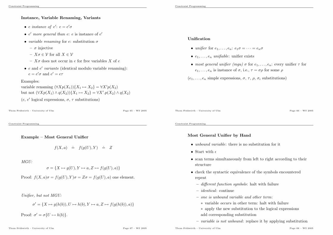
Instance, Variable Renaming, Variants
• e instance of e′: e = e′σ
• e′ more general than e: e is instance of e′
• variable renaming for e: substitution σ
– σ injective
– Xσ ∈ V for all X ∈ V– Xσ does not occur in e for free variables X of e
• e and e′ variants (identical modulo variable renaming):
e = e′σ and e′ = eτ
Examples:
variable renaming (∀Xp(X1)){X1 7→ X2} = ∀X ′p(X2)
but not (∀Xp(X1) ∧ q(X2)){X1 7→ X2} = ∀X ′.p(X2) ∧ q(X2)
(e, e′ logical expressions, σ, τ substitutions)
Thom Fruhwirth – University of Ulm Page 65 – WS 2005
Constraint Programming
Unification
• unifier for e1, . . . , en: e1σ = · · · = enσ
• e1, . . . , en unifiable: unifier exists
• most general unifier (mgu) σ for e1, . . . , en: every unifier τ for
e1, . . . , en is instance of σ, i.e., τ = σρ for some ρ
(e1, . . . , en simple expressions, σ, τ , ρ, σi substitutions)
Thom Fruhwirth – University of Ulm Page 66 – WS 2005
Constraint Programming
Example – Most General Unifier
f(X, a) = f(g(U), Y ) = Z
MGU:
σ = {X 7→ g(U), Y 7→ a, Z 7→ f(g(U), a)}
Proof: f(X, a)σ = f(g(U), Y )σ = Zσ = f(g(U), a) one element.
Unifier, but not MGU:
σ′ = {X 7→ g(h(b)), U 7→ h(b), Y 7→ a, Z 7→ f(g(h(b)), a)}
Proof: σ′ = σ{U 7→ h(b)}.
Thom Fruhwirth – University of Ulm Page 67 – WS 2005
Constraint Programming
Most General Unifier by Hand
• unbound variable: there is no substitution for it
• Start with ǫ
• scan terms simultaneously from left to right according to their
structure
• check the syntactic equivalence of the symbols encountered
repeat
– different function symbols: halt with failure
– identical : continue
– one is unbound variable and other term:
∗ variable occurs in other term: halt with failure
∗ apply the new substitution to the logical expressions
add corresponding substitution
– variable is not unbound : replace it by applying substitution
Thom Fruhwirth – University of Ulm Page 68 – WS 2005
Constraint Programming
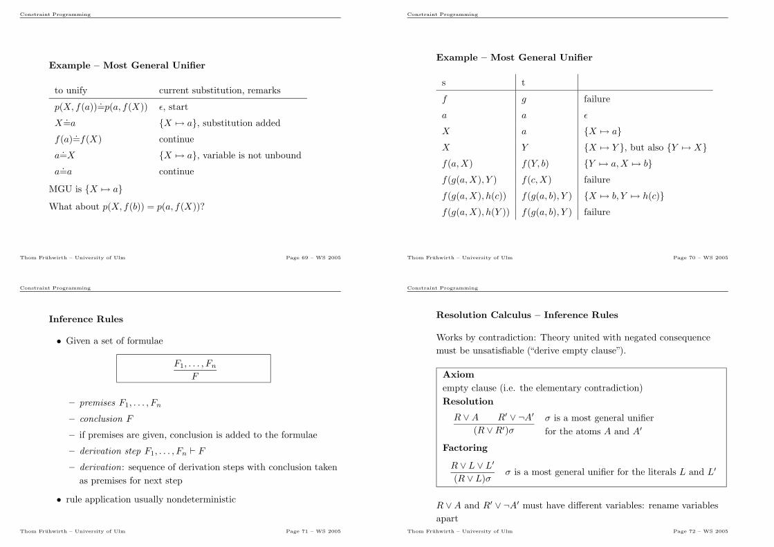
Example – Most General Unifier
to unify current substitution, remarks
p(X, f(a))=p(a, f(X)) ǫ, start
X=a {X 7→ a}, substitution added
f(a)=f(X) continue
a=X {X 7→ a}, variable is not unbound
a=a continue
MGU is {X 7→ a}What about p(X, f(b)) = p(a, f(X))?
Thom Fruhwirth – University of Ulm Page 69 – WS 2005
Constraint Programming
Example – Most General Unifier
s t
f g failure
a a ǫ
X a {X 7→ a}X Y {X 7→ Y }, but also {Y 7→ X}f(a,X) f(Y, b) {Y 7→ a,X 7→ b}f(g(a,X), Y ) f(c,X) failure
f(g(a,X), h(c)) f(g(a, b), Y ) {X 7→ b, Y 7→ h(c)}f(g(a,X), h(Y )) f(g(a, b), Y ) failure
Thom Fruhwirth – University of Ulm Page 70 – WS 2005
Constraint Programming
Inference Rules
• Given a set of formulae
F1, . . . , Fn
F
– premises F1, . . . , Fn
– conclusion F
– if premises are given, conclusion is added to the formulae
– derivation step F1, . . . , Fn ⊢ F– derivation: sequence of derivation steps with conclusion taken
as premises for next step
• rule application usually nondeterministic
Thom Fruhwirth – University of Ulm Page 71 – WS 2005
Constraint Programming
Resolution Calculus – Inference Rules
Works by contradiction: Theory united with negated consequence
must be unsatisfiable (“derive empty clause”).
Axiom
empty clause (i.e. the elementary contradiction)
Resolution
R ∨A R′ ∨ ¬A′
(R ∨R′)σ
σ is a most general unifier
for the atoms A and A′
Factoring
R ∨ L ∨ L′
(R ∨ L)σσ is a most general unifier for the literals L and L′
R ∨A and R′ ∨ ¬A′ must have different variables: rename variables
apartThom Fruhwirth – University of Ulm Page 72 – WS 2005
Constraint Programming
Resolution – Remarks
• resolution rule:
– two clauses C and C ′ instantiated s.t. literal from C and
literal from C ′ complementary
– two instantiated clauses are combined into a new clause
– resolvent added
• factoring rule:
– clause C instantiated, s.t. two literals become equal
– remove one literal
– factor added
Thom Fruhwirth – University of Ulm Page 73 – WS 2005
Constraint Programming
Example – Resolution Calculus
Resolution:p(a,X) ∨ q(X) ¬p(a, b) ∨ r(X)
(q(X) ∨ r(X)){X 7→ b}
Factoring:p(X) ∨ p(b)p(X){X 7→ b}
Thom Fruhwirth – University of Ulm Page 74 – WS 2005
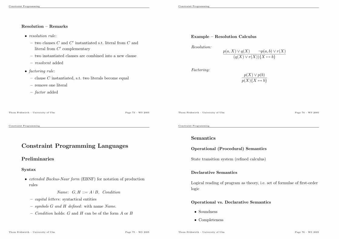
Constraint Programming
Constraint Programming Languages
Preliminaries
Syntax
• extended Backus-Naur form (EBNF) for notation of production
rules
Name: G,H ::= A B, Condition
– capital letters: syntactical entities
– symbols G and H defined : with name Name.
– Condition holds: G and H can be of the form A or B
Thom Fruhwirth – University of Ulm Page 75 – WS 2005
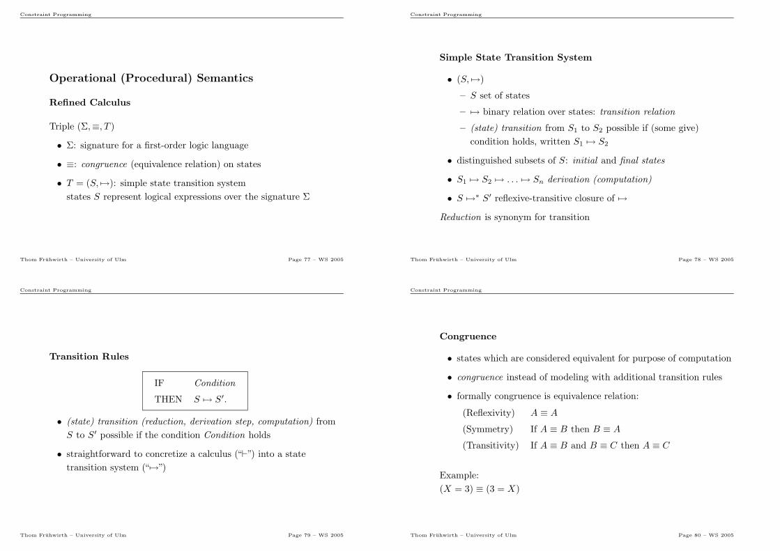
Constraint Programming
Semantics
Operational (Procedural) Semantics
State transition system (refined calculus)
Declarative Semantics
Logical reading of program as theory, i.e. set of formulae of first-order
logic
Operational vs. Declarative Semantics
• Soundness
• Completeness
Thom Fruhwirth – University of Ulm Page 76 – WS 2005
Constraint Programming
Operational (Procedural) Semantics
Refined Calculus
Triple (Σ,≡, T )
• Σ: signature for a first-order logic language
• ≡: congruence (equivalence relation) on states
• T = (S, 7→): simple state transition system
states S represent logical expressions over the signature Σ
Thom Fruhwirth – University of Ulm Page 77 – WS 2005
Constraint Programming
Simple State Transition System
• (S, 7→)
– S set of states
– 7→ binary relation over states: transition relation
– (state) transition from S1 to S2 possible if (some give)
condition holds, written S1 7→ S2
• distinguished subsets of S: initial and final states
• S1 7→ S2 7→ . . . 7→ Sn derivation (computation)
• S 7→∗ S′ reflexive-transitive closure of 7→
Reduction is synonym for transition
Thom Fruhwirth – University of Ulm Page 78 – WS 2005
Constraint Programming
Transition Rules
IF Condition
THEN S 7→ S′.
• (state) transition (reduction, derivation step, computation) from
S to S′ possible if the condition Condition holds
• straightforward to concretize a calculus (“⊢”) into a state
transition system (“7→”)
Thom Fruhwirth – University of Ulm Page 79 – WS 2005
Constraint Programming
Congruence
• states which are considered equivalent for purpose of computation
• congruence instead of modeling with additional transition rules
• formally congruence is equivalence relation:
(Reflexivity) A ≡ A(Symmetry) If A ≡ B then B ≡ A(Transitivity) If A ≡ B and B ≡ C then A ≡ C
Example:
(X = 3) ≡ (3 = X)
Thom Fruhwirth – University of Ulm Page 80 – WS 2005
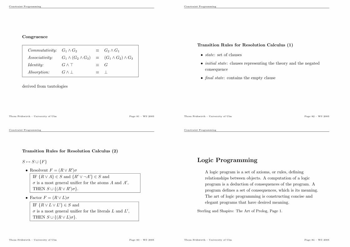
Constraint Programming
Congruence
Commutativity: G1 ∧G2 ≡ G2 ∧G1
Associativity: G1 ∧ (G2 ∧G3) ≡ (G1 ∧G2) ∧G3
Identity: G ∧ ⊤ ≡ G
Absorption: G ∧ ⊥ ≡ ⊥
derived from tautologies
Thom Fruhwirth – University of Ulm Page 81 – WS 2005
Constraint Programming
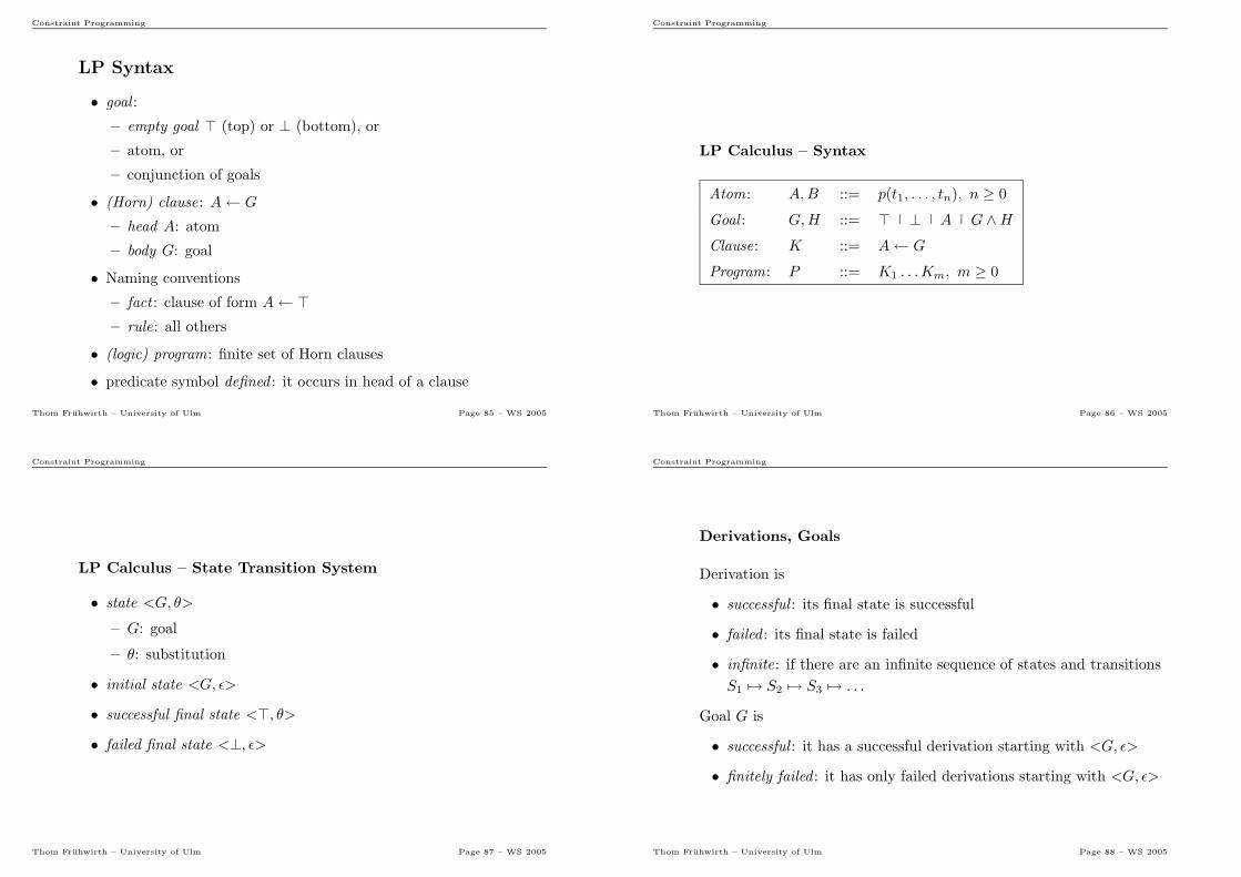
Transition Rules for Resolution Calculus (1)
• state: set of clauses
• initial state: clauses representing the theory and the negated
consequence
• final state: contains the empty clause
Thom Fruhwirth – University of Ulm Page 82 – WS 2005
Constraint Programming
Transition Rules for Resolution Calculus (2)
S 7→ S ∪ {F}
• Resolvent F = (R ∨R′)σ
IF {R ∨A} ∈ S and {R′ ∨ ¬A′} ∈ S and
σ is a most general unifier for the atoms A and A′,
THEN S ∪ {(R ∨R′)σ}.
• Factor F = (R ∨ L)σ
IF {R ∨ L ∨ L′} ∈ S and
σ is a most general unifier for the literals L and L′,
THEN S ∪ {(R ∨ L)σ}.
Thom Fruhwirth – University of Ulm Page 83 – WS 2005
Constraint Programming
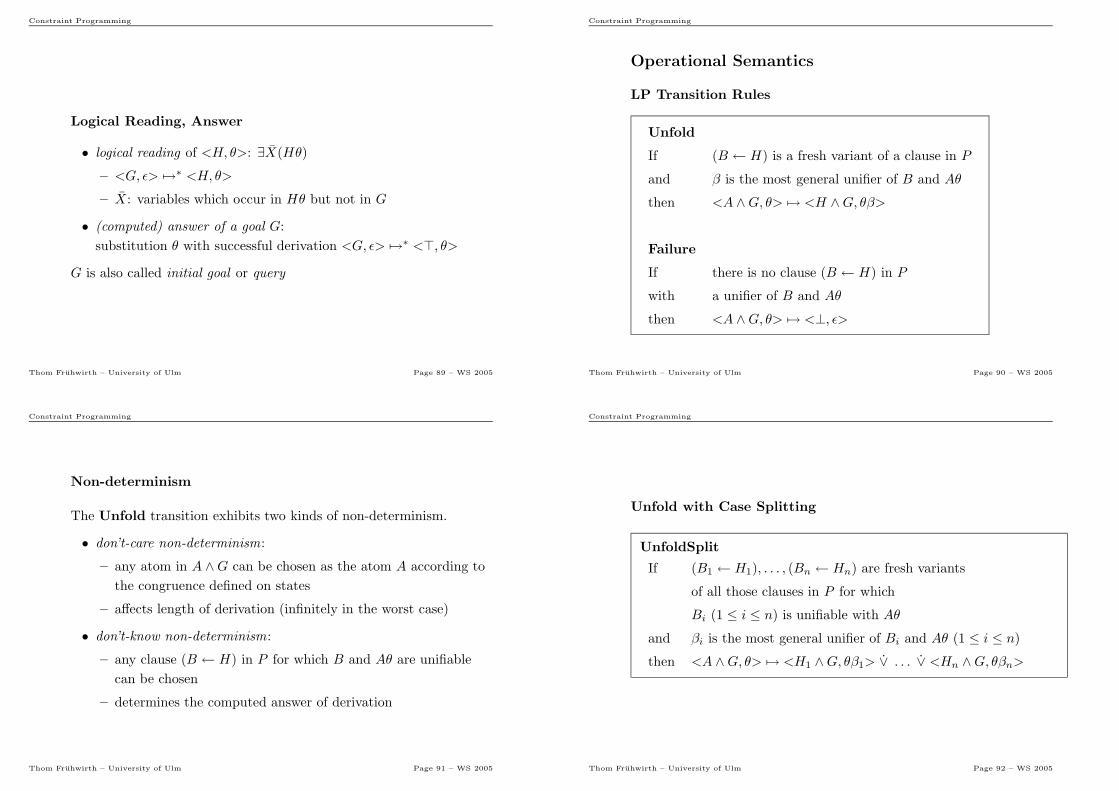
Logic Programming
A logic program is a set of axioms, or rules, defining
relationships between objects. A computation of a logic
program is a deduction of consequences of the program. A
program defines a set of consequences, which is its meaning.
The art of logic programming is constructing concise and
elegant programs that have desired meaning.
Sterling and Shapiro: The Art of Prolog, Page 1.
Thom Fruhwirth – University of Ulm Page 84 – WS 2005
Constraint Programming
LP Syntax
• goal :
– empty goal ⊤ (top) or ⊥ (bottom), or
– atom, or
– conjunction of goals
• (Horn) clause: A← G
– head A: atom
– body G: goal
• Naming conventions
– fact : clause of form A← ⊤– rule: all others
• (logic) program: finite set of Horn clauses
• predicate symbol defined : it occurs in head of a clause
Thom Fruhwirth – University of Ulm Page 85 – WS 2005
Constraint Programming
LP Calculus – Syntax
Atom: A,B ::= p(t1, . . . , tn), n ≥ 0
Goal : G,H ::= ⊤ ⊥ A G ∧HClause: K ::= A← G
Program: P ::= K1 . . .Km, m ≥ 0
Thom Fruhwirth – University of Ulm Page 86 – WS 2005
Constraint Programming
LP Calculus – State Transition System
• state <G, θ>
– G: goal
– θ: substitution
• initial state <G, ǫ>
• successful final state <⊤, θ>
• failed final state <⊥, ǫ>
Thom Fruhwirth – University of Ulm Page 87 – WS 2005
Constraint Programming
Derivations, Goals
Derivation is
• successful : its final state is successful
• failed : its final state is failed
• infinite: if there are an infinite sequence of states and transitions
S1 7→ S2 7→ S3 7→ . . .
Goal G is
• successful : it has a successful derivation starting with <G, ǫ>
• finitely failed : it has only failed derivations starting with <G, ǫ>
Thom Fruhwirth – University of Ulm Page 88 – WS 2005
Constraint Programming
Logical Reading, Answer
• logical reading of <H, θ>: ∃X(Hθ)
– <G, ǫ> 7→∗ <H, θ>
– X: variables which occur in Hθ but not in G
• (computed) answer of a goal G:
substitution θ with successful derivation <G, ǫ> 7→∗ <⊤, θ>
G is also called initial goal or query
Thom Fruhwirth – University of Ulm Page 89 – WS 2005
Constraint Programming
Operational Semantics
LP Transition Rules
Unfold
If (B ← H) is a fresh variant of a clause in P
and β is the most general unifier of B and Aθ
then <A ∧G, θ> 7→ <H ∧G, θβ>
Failure
If there is no clause (B ← H) in P
with a unifier of B and Aθ
then <A ∧G, θ> 7→ <⊥, ǫ>
Thom Fruhwirth – University of Ulm Page 90 – WS 2005
Constraint Programming
Non-determinism
The Unfold transition exhibits two kinds of non-determinism.
• don’t-care non-determinism:
– any atom in A ∧G can be chosen as the atom A according to
the congruence defined on states
– affects length of derivation (infinitely in the worst case)
• don’t-know non-determinism:
– any clause (B ← H) in P for which B and Aθ are unifiable
can be chosen
– determines the computed answer of derivation
Thom Fruhwirth – University of Ulm Page 91 – WS 2005
Constraint Programming
Unfold with Case Splitting
UnfoldSplit
If (B1 ← H1), . . . , (Bn ← Hn) are fresh variants
of all those clauses in P for which
Bi (1 ≤ i ≤ n) is unifiable with Aθ
and βi is the most general unifier of Bi and Aθ (1 ≤ i ≤ n)
then <A ∧G, θ> 7→ <H1 ∧G, θβ1> ∨ . . . ∨ <Hn ∧G, θβn>
Thom Fruhwirth – University of Ulm Page 92 – WS 2005
Constraint Programming
SLD Resolution
• selection strategy : textual order of clauses and atoms in a
program
• (chronological) backtracking (backtrack search)
• left-to-right, depth-first exploration of the search tree
• efficient implementation using a stack-based approach
• can get trapped in infinite derivations
(but breadth-first search far too inefficient)
Thom Fruhwirth – University of Ulm Page 93 – WS 2005
Constraint Programming
Example - Accessibility in DAG
a
��
// c
��
b // d // e
edge(a,b) ← ⊤ (e1)
edge(a,c) ← ⊤ (e2)
edge(b,d) ← ⊤ (e3)
edge(c,d) ← ⊤ (e4)
edge(d,e) ← ⊤ (e5)
path(Start,End) ← edge(Start,End) (p1)
path(Start,End) ← edge(Start,Node) ∧ path(Node,End) (p2)
Thom Fruhwirth – University of Ulm Page 94 – WS 2005
Constraint Programming
Example - Accessibility in DAG (cont)
a
��
// c
��
b // d // e
<path(b, Y), ε>
7→Unfold (p1) <edge(S, E), {S← b, E← Y}>7→Unfold (e3) <⊤, {S← b, E← d, Y← d}>
With the second rule p2 for path selected:
<path(b, Y), ε>
7→Unfold (p2) <edge(S, N) ∧ path(N, E), {S← b, E← Y}>7→Unfold (e3) <path(N, E), {S← b, E← Y, N← d}>7→Unfold (p1) <edge(N, E), {S← b, E← Y, N← d}>7→Unfold (e5) <⊤, {S← b, E← e, N← d, Y← e}>
Thom Fruhwirth – University of Ulm Page 95 – WS 2005
Constraint Programming
Example - Accessibility in DAG (cont 2)
a
��
// c
��
b // d // e
Partial search tree:
<path(b, Y), ε>
p1
yyrrrrrrrrrrp2
((QQQQQQQQQQQQQ
<edge(S, E), {S← b, E← Y}>
e3
��
<edge(S, N) ∧ path(N, E), {S← b, E← Y}>... ...
��<⊤, {S← b, E← d, Y← d}> . . .
Thom Fruhwirth – University of Ulm Page 96 – WS 2005
Constraint Programming
Example - Accessibility in DAG (cont 3)
a
��
// c
��
b // d // e
With the first rule:
<path(f, g), ε>
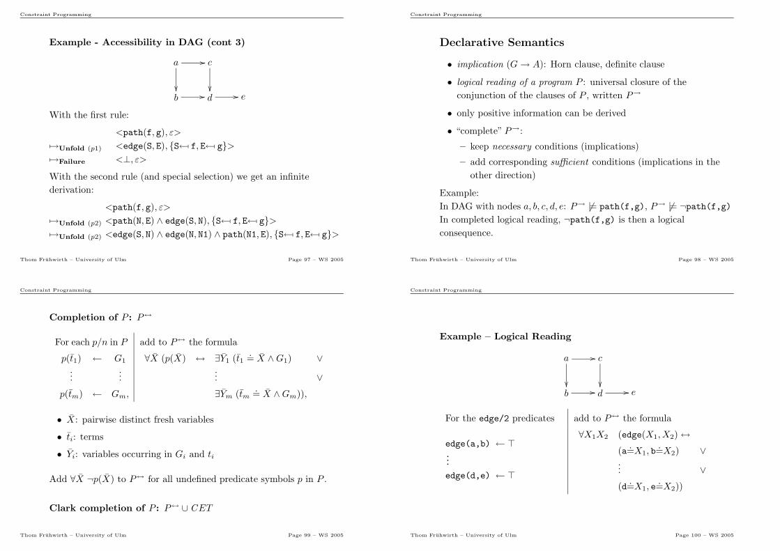
7→Unfold (p1) <edge(S, E), {S← f, E← g}>7→Failure <⊥, ε>With the second rule (and special selection) we get an infinite
derivation:
<path(f, g), ε>
7→Unfold (p2) <path(N, E) ∧ edge(S, N), {S← f, E← g}>7→Unfold (p2) <edge(S, N) ∧ edge(N, N1) ∧ path(N1, E), {S← f, E← g}>
Thom Fruhwirth – University of Ulm Page 97 – WS 2005
Constraint Programming
Declarative Semantics
• implication (G→ A): Horn clause, definite clause
• logical reading of a program P : universal closure of the
conjunction of the clauses of P , written P→
• only positive information can be derived
• “complete” P→:
– keep necessary conditions (implications)
– add corresponding sufficient conditions (implications in the
other direction)
Example:
In DAG with nodes a, b, c, d, e: P→ 6|= path(f,g), P→ 6|= ¬path(f,g)In completed logical reading, ¬path(f,g) is then a logical
consequence.
Thom Fruhwirth – University of Ulm Page 98 – WS 2005
Constraint Programming
Completion of P : P↔
For each p/n in P add to P↔ the formula
p(t1) ← G1
......
p(tm) ← Gm,
∀X (p(X) ↔ ∃Y1 (t1.= X ∧G1) ∨
... ∨∃Ym (tm
.= X ∧Gm)),
• X: pairwise distinct fresh variables
• ti: terms
• Yi: variables occurring in Gi and ti
Add ∀X ¬p(X) to P↔ for all undefined predicate symbols p in P .
Clark completion of P : P↔ ∪ CET
Thom Fruhwirth – University of Ulm Page 99 – WS 2005
Constraint Programming
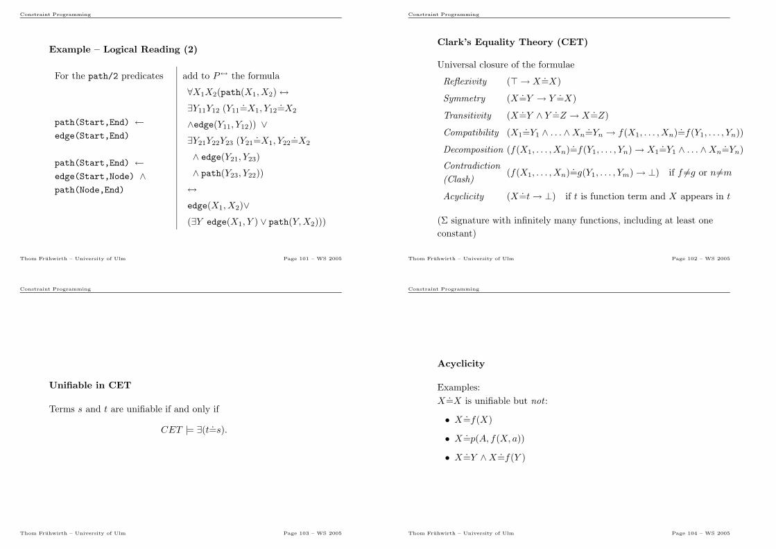
Example – Logical Reading
a
��
// c
��
b // d // e
For the edge/2 predicates add to P↔ the formula
edge(a,b) ← ⊤...
edge(d,e) ← ⊤
∀X1X2 (edge(X1, X2)↔(a=X1, b=X2) ∨... ∨(d=X1, e=X2))
Thom Fruhwirth – University of Ulm Page 100 – WS 2005
Constraint Programming
Example – Logical Reading (2)
For the path/2 predicates add to P↔ the formula
path(Start,End) ←edge(Start,End)
path(Start,End) ←edge(Start,Node) ∧path(Node,End)
∀X1X2(path(X1, X2)↔∃Y11Y12 (Y11=X1, Y12=X2
∧edge(Y11, Y12)) ∨∃Y21Y22Y23 (Y21=X1, Y22=X2
∧ edge(Y21, Y23)
∧ path(Y23, Y22))
↔edge(X1, X2)∨(∃Y edge(X1, Y ) ∨ path(Y,X2)))
Thom Fruhwirth – University of Ulm Page 101 – WS 2005
Constraint Programming
Clark’s Equality Theory (CET)
Universal closure of the formulae
Reflexivity (⊤ → X=X)
Symmetry (X=Y → Y =X)
Transitivity (X=Y ∧ Y =Z → X=Z)
Compatibility (X1=Y1 ∧ . . . ∧Xn=Yn → f(X1, . . . , Xn)=f(Y1, . . . , Yn))
Decomposition (f(X1, . . . , Xn)=f(Y1, . . . , Yn)→ X1=Y1 ∧ . . . ∧Xn=Yn)
Contradiction
(Clash)(f(X1, . . . , Xn)=g(Y1, . . . , Ym)→ ⊥) if f 6=g or n6=m
Acyclicity (X=t→ ⊥) if t is function term and X appears in t
(Σ signature with infinitely many functions, including at least one
constant)
Thom Fruhwirth – University of Ulm Page 102 – WS 2005
Constraint Programming
Unifiable in CET
Terms s and t are unifiable if and only if
CET |= ∃(t=s).
Thom Fruhwirth – University of Ulm Page 103 – WS 2005
Constraint Programming
Acyclicity
Examples:
X=X is unifiable but not :
• X=f(X)
• X=p(A, f(X, a))
• X=Y ∧X=f(Y )
Thom Fruhwirth – University of Ulm Page 104 – WS 2005
Constraint Programming
Soundness and Completeness
Successful derivations
• Soundness:
If θ is a computed answer of G, then P↔ ∪ CET |= ∀Gθ.
• Completeness:
If P↔ ∪ CET |= ∀Gθ, then a computed answer σ of G exists,
such that θ = σβ.
(P logic program, G goal, θ substitution)
Thom Fruhwirth – University of Ulm Page 105 – WS 2005
Constraint Programming
Failed Derivations
• Fair Derivation:
Either fails or each atom appearing in the derivation is selected
after finitely many reductions.
• Soundness and Completeness:
Any fair derivation starting with <G, ǫ> fails finitely if and only
if
P↔ ∪ CET |= ¬∃G.Remarks:
• not valid without CET
• SLD resolution not fair
(P logic program, G goal)
Thom Fruhwirth – University of Ulm Page 106 – WS 2005
Constraint Programming
Constraint Logic Programming (CLP)
• Constraint Satisfaction Problems (CSP)
– artificial intelligence (1970s)
– e.g. X∈{1, 2} ∧ Y ∈{1, 2} ∧ Z∈{1, 2} ∧X=Y ∧X 6=Z ∧ Y >Z
• Constraint Logic Programming (CLP)
– developed in the mid-1980s
– two declarative paradigms: constraint solving and logic
programming
– more expressive, flexible, and in general more efficient than
logic programs
– e.g. X − Y = 3 ∧ X + Y = 7 leads to X = 5 ∧ Y = 2
– e.g. X < Y ∧ Y < X fails without the need to know values
Thom Fruhwirth – University of Ulm Page 107 – WS 2005
Constraint Programming
Early history of constraint-based programming
1963 I. Sutherland, Sketchpad, graphic system for geometric drawing
1970 U. Montanari, Pisa, Constraint networks
1970 R.E. Fikes, REF-ARF, language for integer linear equations
1972 A. Colmerauer, U. Marseille, and R. Kowalski, IC London, Prolog
1977 A.K. Mackworth, Constraint networks algorithms
1978 J.-L. Lauriere, Alice, language for combinatorial problems
1979 A. Borning, Thinglab, interactive graphics
1980 G.L. Steele, Constraints, first constraint-based language, in LISP
1982 A. Colmerauer, Prolog II, U. Marseille, equality constraints
1984 Eclipse Prolog, ECRC Munich, later IC-PARC London
1985 SICStus Prolog, Swedish Institute of Computer Science (SICS)
Thom Fruhwirth – University of Ulm Page 108 – WS 2005
Constraint Programming
Early history of constraint-based programming (cont)
1987 H. Ait-Kaci, U. Austin, Life, equality constraints
1987 J. Jaffar and J.L. Lassez, CLP(X) - Scheme, Monash U. Melbourne
1987 J. Jaffar, CLP(ℜ), Monash U. Melbourne, linear polynomials
1988 P. v. Hentenryck, CHIP, ECRC Munich, finite domains, Booleans
1988 P. Voda, Trilogy, Vancouver, integer arithmetics
1988 W. Older, BNR-Prolog, Bell-Northern Research Ottawa, intervals
1988 A. Aiba, CAL, ICOT Tokyo, non-linear equation systems
1988 W. Leler, Bertrand, term rewriting for defining constraints
1988 A. Colmerauer, Prolog III, U. Marseille, list constraints and more
Thom Fruhwirth – University of Ulm Page 109 – WS 2005
Constraint Programming
CLP Syntax vs. LP Syntax
• signature augmented with constraint symbols
• consistent first-order constraint theory (CT )
• at least constraint symbols true and false
• syntactic equality = as constraints (by including CET into CT)
• constraints handled by predefined, given constraint solver
Thom Fruhwirth – University of Ulm Page 110 – WS 2005
Constraint Programming
CLP Syntax (cont)
• atom: expression p(t1, . . . , tn), with predicate symbol p/n
• atomic constraint : expression c(t1, . . . , tn), with n-ary constraint
symbol c/n
• constraint :
– atomic constraint, or
– conjunction of constraints
• goal :
– ⊤ (top), or ⊥ (bottom), or
– atom, or an atomic constraint, or
– conjunction of goals
• (CL) clause: A← G, with atom A and goal G
• CL program: finite set of CL clauses
Thom Fruhwirth – University of Ulm Page 111 – WS 2005
Constraint Programming
CLP Syntax – Summary
Atom: A,B ::= p(t1, . . . , tn), n ≥ 0
Constraint : C,D ::= c(t1, . . . , tn) C ∧D, n ≥ 0
Goal : G,H ::= ⊤ ⊥ A C G ∧HCL Clause: K ::= A← G
CL Program: P ::= K1 . . .Km, m ≥ 0
Thom Fruhwirth – University of Ulm Page 112 – WS 2005
Constraint Programming
CLP State Transition System
• state <G,C>: G goal (store), C constraint (store)
• initial state: <G, true>
• successful final state: <⊤, C> and C is different from false
• failed final state: <G, false>
• successful and failed derivations and goals: as in LP calculus
Thom Fruhwirth – University of Ulm Page 113 – WS 2005
Constraint Programming
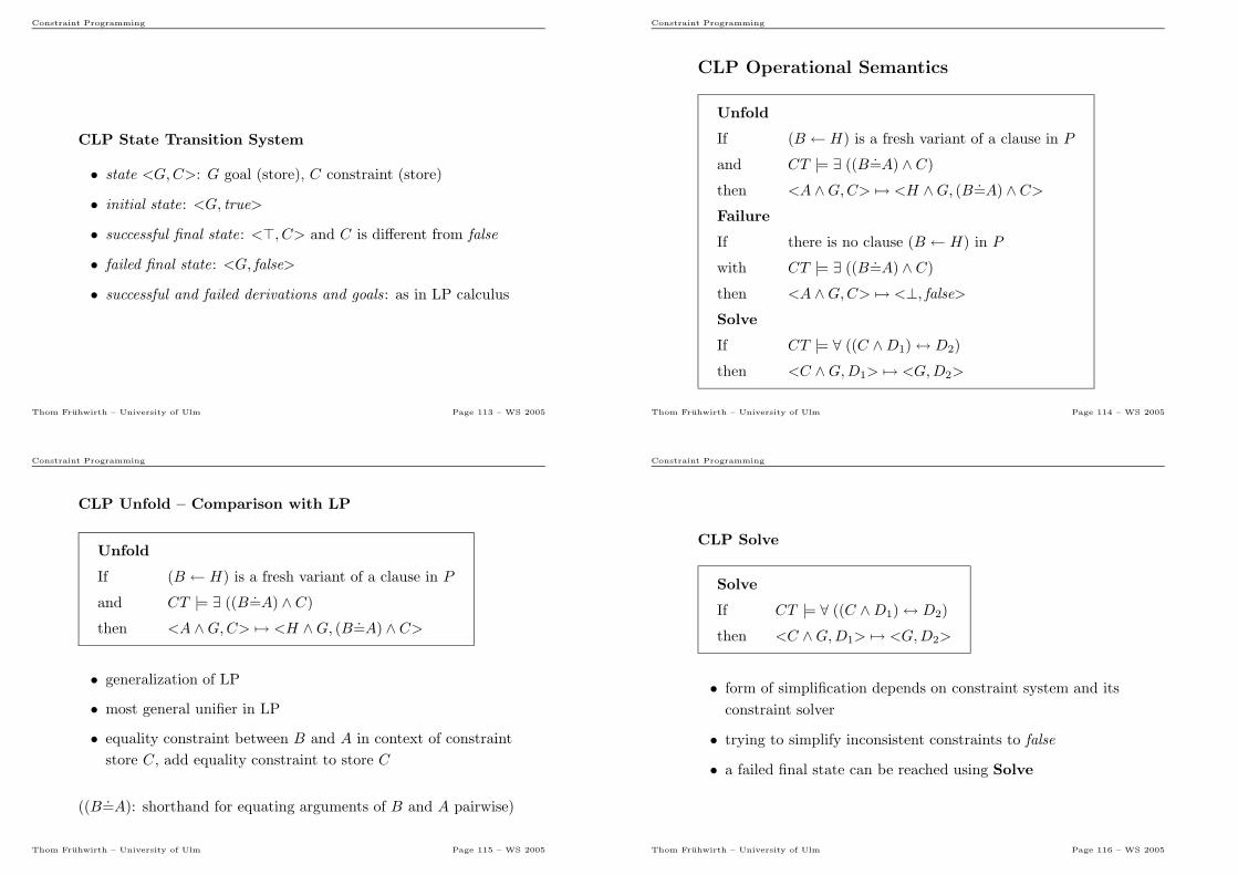
CLP Operational Semantics
Unfold
If (B ← H) is a fresh variant of a clause in P
and CT |= ∃ ((B.=A) ∧ C)
then <A ∧G,C> 7→ <H ∧G, (B .=A) ∧ C>
Failure
If there is no clause (B ← H) in P
with CT |= ∃ ((B.=A) ∧ C)
then <A ∧G,C> 7→ <⊥, false>Solve
If CT |= ∀ ((C ∧D1)↔ D2)
then <C ∧G,D1> 7→ <G,D2>
Thom Fruhwirth – University of Ulm Page 114 – WS 2005
Constraint Programming
CLP Unfold – Comparison with LP
Unfold
If (B ← H) is a fresh variant of a clause in P
and CT |= ∃ ((B.=A) ∧ C)
then <A ∧G,C> 7→ <H ∧G, (B .=A) ∧ C>
• generalization of LP
• most general unifier in LP
• equality constraint between B and A in context of constraint
store C, add equality constraint to store C
((B=A): shorthand for equating arguments of B and A pairwise)
Thom Fruhwirth – University of Ulm Page 115 – WS 2005
Constraint Programming
CLP Solve
Solve
If CT |= ∀ ((C ∧D1)↔ D2)
then <C ∧G,D1> 7→ <G,D2>
• form of simplification depends on constraint system and its
constraint solver
• trying to simplify inconsistent constraints to false
• a failed final state can be reached using Solve
Thom Fruhwirth – University of Ulm Page 116 – WS 2005
Constraint Programming
CLP State Transition System (vs. LP)
• like in LP, two degrees of non-determinism in the calculus
(selecting the goal and selecting the clause)
• like in LP, search trees (mostly SLD resolution)
• LP : accumulate and compose substitutions
CLP : accumulate and simplify constraints
• like substitutions, constraints never removed from constraint
store (information increases monotonically during derivations)
Thom Fruhwirth – University of Ulm Page 117 – WS 2005
Constraint Programming
CLP as Extension to LP
• derivation in LP can be expressed as CLP derivations:
– LP : substitution {X1 7→t1, . . . , Xn 7→tn}– CLP : equality constraints: X1
.=t1 ∧ . . . ∧Xn
.=tn
• CLP generalizes form of answers.
– LP answer : substitution
– CLP answer : constraint
• Constraints summarize several (even infinitely many) LP answers
into one (intensional) answer, e.g.,
– X+Y≥3 ∧ X+Y≤3 simplified to
– X+Y.= 3
– variables do not need to have a value
Thom Fruhwirth – University of Ulm Page 118 – WS 2005
Constraint Programming
CLP Logical Reading, Answer Constraint
• logical reading of a state <H,C>: ∃X(H ∧ C)
– <G, true> 7→∗ <H,C>
– X: variables which occur in H or C but not in G
• answer (constraint) of a goal G:
logical reading of final state of derivation starting with <G, true>
Answer constraints of final states:
• 〈⊤, C〉 is true as (∃X⊤ ∧ C)⇔ ∃XC
• 〈G, false〉 is false as (∃XG ∧ false)⇔ false
Thom Fruhwirth – University of Ulm Page 119 – WS 2005
Constraint Programming
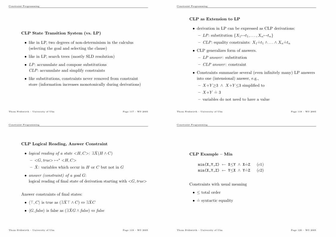
CLP Example – Min
min(X,Y,Z) ← X≤Y ∧ X.=Z (c1)
min(X,Y,Z) ← Y≤X ∧ Y.=Z (c2)
Constraints with usual meaning
• ≤ total order
• .= syntactic equality
Thom Fruhwirth – University of Ulm Page 120 – WS 2005
Constraint Programming
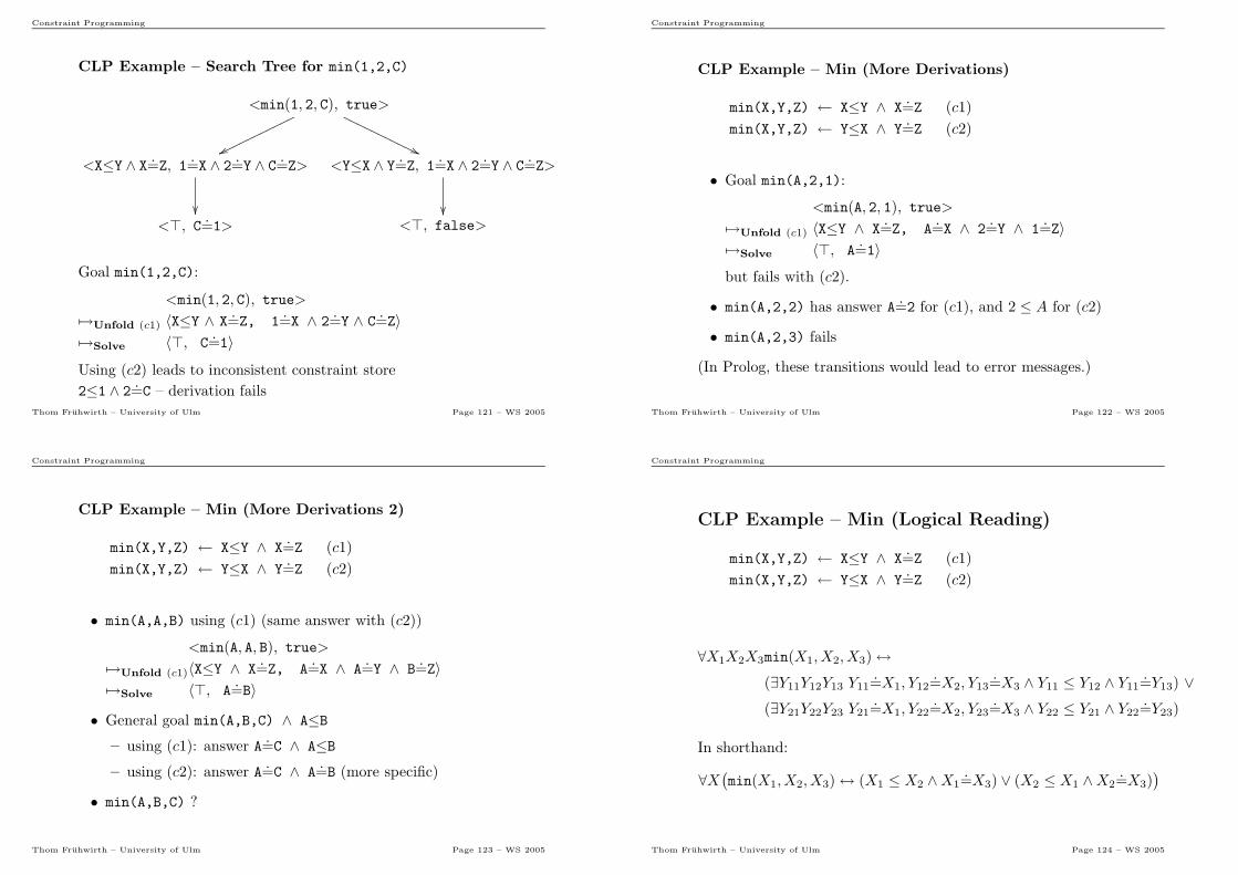
CLP Example – Search Tree for min(1,2,C)
<min(1, 2, C), true>
wwooooooooooo
''OOOOOOOOOOO
<X≤Y ∧ X .=Z, 1.=X ∧ 2 .=Y ∧ C .=Z>
��
<Y≤X ∧ Y .=Z, 1.=X ∧ 2 .=Y ∧ C .=Z>
��
<⊤, C .=1> <⊤, false>
Goal min(1,2,C):
<min(1, 2, C), true>
7→Unfold (c1) 〈X≤Y ∧ X.=Z, 1
.=X ∧ 2
.=Y ∧ C
.=Z〉
7→Solve 〈⊤, C.=1〉
Using (c2) leads to inconsistent constraint store
2≤1 ∧ 2 .=C – derivation fails
Thom Fruhwirth – University of Ulm Page 121 – WS 2005
Constraint Programming
CLP Example – Min (More Derivations)
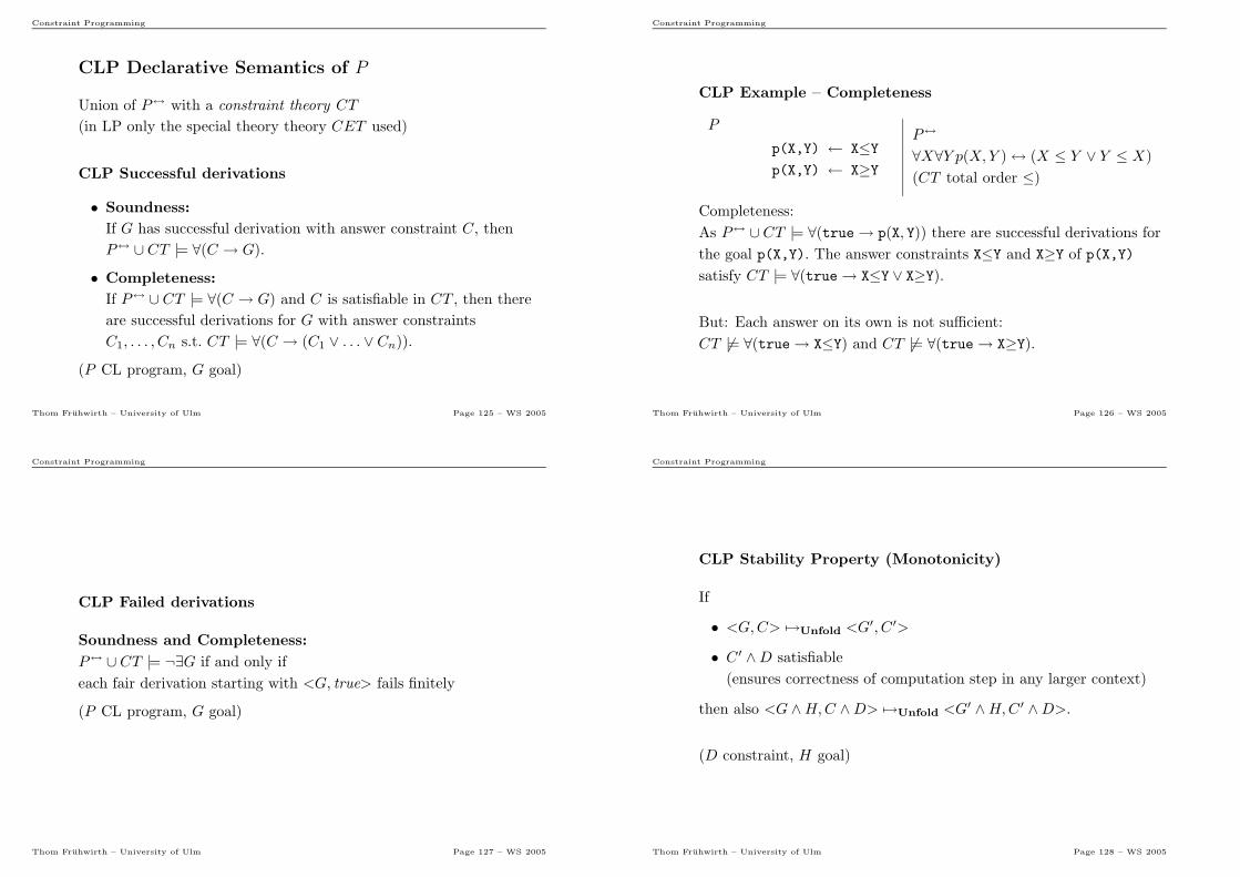
min(X,Y,Z) ← X≤Y ∧ X.=Z (c1)
min(X,Y,Z) ← Y≤X ∧ Y.=Z (c2)
• Goal min(A,2,1):
<min(A, 2, 1), true>
7→Unfold (c1) 〈X≤Y ∧ X.=Z, A
.=X ∧ 2
.=Y ∧ 1
.=Z〉
7→Solve 〈⊤, A.=1〉
but fails with (c2).
• min(A,2,2) has answer A.=2 for (c1), and 2 ≤ A for (c2)
• min(A,2,3) fails
(In Prolog, these transitions would lead to error messages.)
Thom Fruhwirth – University of Ulm Page 122 – WS 2005
Constraint Programming
CLP Example – Min (More Derivations 2)
min(X,Y,Z) ← X≤Y ∧ X.=Z (c1)
min(X,Y,Z) ← Y≤X ∧ Y.=Z (c2)
• min(A,A,B) using (c1) (same answer with (c2))
<min(A, A, B), true>
7→Unfold (c1)〈X≤Y ∧ X.=Z, A
.=X ∧ A
.=Y ∧ B
.=Z〉
7→Solve 〈⊤, A.=B〉
• General goal min(A,B,C) ∧ A≤B– using (c1): answer A=C ∧ A≤B– using (c2): answer A=C ∧ A=B (more specific)
• min(A,B,C) ?
Thom Fruhwirth – University of Ulm Page 123 – WS 2005
Constraint Programming
CLP Example – Min (Logical Reading)
min(X,Y,Z) ← X≤Y ∧ X.=Z (c1)
min(X,Y,Z) ← Y≤X ∧ Y.=Z (c2)
∀X1X2X3min(X1, X2, X3)↔(∃Y11Y12Y13 Y11=X1, Y12=X2, Y13=X3 ∧ Y11 ≤ Y12 ∧ Y11=Y13) ∨(∃Y21Y22Y23 Y21=X1, Y22=X2, Y23=X3 ∧ Y22 ≤ Y21 ∧ Y22=Y23)
In shorthand:
∀X(min(X1, X2, X3)↔ (X1 ≤ X2 ∧X1=X3) ∨ (X2 ≤ X1 ∧X2=X3)
)
Thom Fruhwirth – University of Ulm Page 124 – WS 2005
Constraint Programming
CLP Declarative Semantics of P
Union of P↔ with a constraint theory CT
(in LP only the special theory theory CET used)
CLP Successful derivations
• Soundness:
If G has successful derivation with answer constraint C, then
P↔ ∪ CT |= ∀(C → G).
• Completeness:
If P↔ ∪ CT |= ∀(C → G) and C is satisfiable in CT , then there
are successful derivations for G with answer constraints
C1, . . . , Cn s.t. CT |= ∀(C → (C1 ∨ . . . ∨ Cn)).
(P CL program, G goal)
Thom Fruhwirth – University of Ulm Page 125 – WS 2005
Constraint Programming
CLP Example – Completeness
P
p(X,Y) ← X≤Yp(X,Y) ← X≥Y
P↔
∀X∀Y p(X,Y )↔ (X ≤ Y ∨ Y ≤ X)
(CT total order ≤)
Completeness:
As P↔ ∪ CT |= ∀(true→ p(X, Y)) there are successful derivations for
the goal p(X,Y). The answer constraints X≤Y and X≥Y of p(X,Y)
satisfy CT |= ∀(true→ X≤Y ∨ X≥Y).
But: Each answer on its own is not sufficient:
CT 6|= ∀(true→ X≤Y) and CT 6|= ∀(true→ X≥Y).
Thom Fruhwirth – University of Ulm Page 126 – WS 2005
Constraint Programming
CLP Failed derivations
Soundness and Completeness:
P↔ ∪ CT |= ¬∃G if and only if
each fair derivation starting with <G, true> fails finitely
(P CL program, G goal)
Thom Fruhwirth – University of Ulm Page 127 – WS 2005
Constraint Programming
CLP Stability Property (Monotonicity)
If
• <G,C> 7→Unfold <G′, C′>
• C′ ∧D satisfiable
(ensures correctness of computation step in any larger context)
then also <G ∧H,C ∧D> 7→Unfold <G′ ∧H,C ′ ∧D>.
(D constraint, H goal)
Thom Fruhwirth – University of Ulm Page 128 – WS 2005
Constraint Programming
CLP vs. LP – Overview
• generate-and-test in LP : impractical, facts used in passive
manner only
• constrain-and-generate in CLP : use facts in active manner to
reduce the search space (constraints)
• combination of
– LP languages: declarative, for arbitrary predicates,
non-deterministic
– constraint solvers: declarative, efficient for special predicates,
deterministic
• combination of search with constraints solving particularly useful
Thom Fruhwirth – University of Ulm Page 129 – WS 2005
Constraint Programming
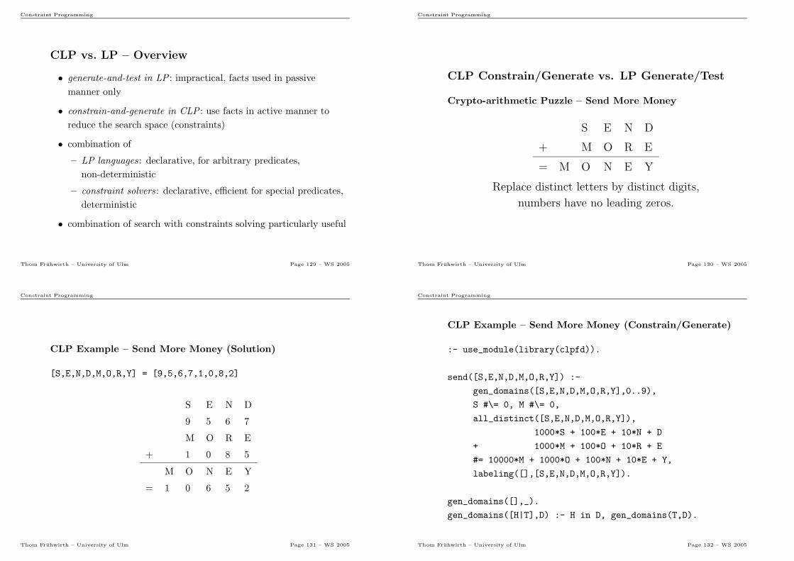
CLP Constrain/Generate vs. LP Generate/Test
Crypto-arithmetic Puzzle – Send More Money
S E N D
+ M O R E
= M O N E Y
Replace distinct letters by distinct digits,
numbers have no leading zeros.
Thom Fruhwirth – University of Ulm Page 130 – WS 2005
Constraint Programming
CLP Example – Send More Money (Solution)
[S,E,N,D,M,O,R,Y] = [9,5,6,7,1,0,8,2]
S E N D
9 5 6 7
M O R E
+ 1 0 8 5
M O N E Y
= 1 0 6 5 2
Thom Fruhwirth – University of Ulm Page 131 – WS 2005
Constraint Programming
CLP Example – Send More Money (Constrain/Generate)
:- use_module(library(clpfd)).
send([S,E,N,D,M,O,R,Y]) :-
gen_domains([S,E,N,D,M,O,R,Y],0..9),
S #\= 0, M #\= 0,
all_distinct([S,E,N,D,M,O,R,Y]),
1000*S + 100*E + 10*N + D
+ 1000*M + 100*O + 10*R + E
#= 10000*M + 1000*O + 100*N + 10*E + Y,
labeling([],[S,E,N,D,M,O,R,Y]).
gen_domains([],_).
gen_domains([H|T],D) :- H in D, gen_domains(T,D).
Thom Fruhwirth – University of Ulm Page 132 – WS 2005
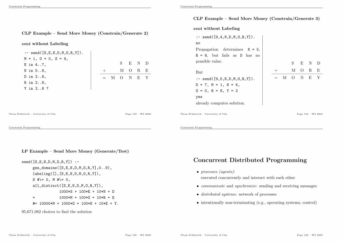
Constraint Programming
CLP Example – Send More Money (Constrain/Generate 2)
send without Labeling
:- send([S,E,N,D,M,O,R,Y]).
M = 1, O = 0, S = 9,
E in 4..7,
N in 5..8,
D in 2..8,
R in 2..8,
Y in 2..8 ?
S E N D
+ M O R E
= M O N E Y
Thom Fruhwirth – University of Ulm Page 133 – WS 2005
Constraint Programming
CLP Example – Send More Money (Constrain/Generate 3)
send without Labeling
:- send([9,4,N,D,M,O,R,Y]).
no
Propagation determines N = 5,
R = 8, but fails as D has no
possible value.
But
:- send([9,5,N,D,M,O,R,Y]).
D = 7, M = 1, N = 6,
O = 0, R = 8, Y = 2
yes
already computes solution.
S E N D
+ M O R E
= M O N E Y
Thom Fruhwirth – University of Ulm Page 134 – WS 2005
Constraint Programming
LP Example – Send More Money (Generate/Test)
send([S,E,N,D,M,O,R,Y]) :-
gen_domains([S,E,N,D,M,O,R,Y],0..9),
labeling([],[S,E,N,D,M,O,R,Y]),
S #\= 0, M #\= 0,
all_distinct([S,E,N,D,M,O,R,Y]),
1000*S + 100*E + 10*N + D
+ 1000*M + 100*O + 10*R + E
#= 10000*M + 1000*O + 100*N + 10*E + Y.
95,671,082 choices to find the solution
Thom Fruhwirth – University of Ulm Page 135 – WS 2005
Constraint Programming
Concurrent Distributed Programming
• processes (agents):
executed concurrently and interact with each other
• communicate and synchronize: sending and receiving messages
• distributed systems: network of processes
• intentionally non-terminating (e.g., operating systems, control)
Thom Fruhwirth – University of Ulm Page 136 – WS 2005
Constraint Programming
Concurrent Constraint Logic
Programming (CCLP)
• integrates ideas from concurrent LP and CLP
• communication: common constraint store (blackboard)
• processes: predicates
• (partial) messages: constraints
• communication channels: variables
• running processes: goals that place and check constraints on
shared variables
Thom Fruhwirth – University of Ulm Page 137 – WS 2005
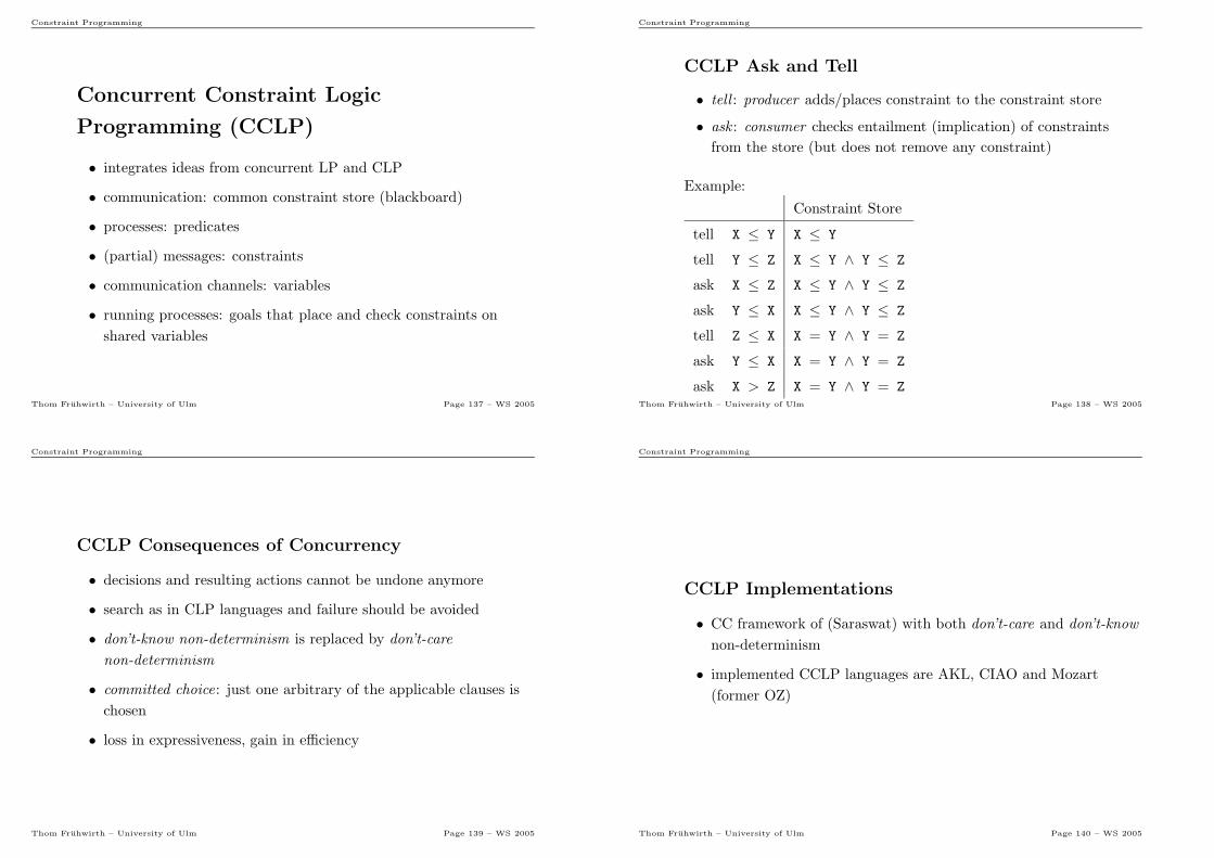
Constraint Programming
CCLP Ask and Tell
• tell : producer adds/places constraint to the constraint store
• ask : consumer checks entailment (implication) of constraints
from the store (but does not remove any constraint)
Example:
Constraint Store
tell X ≤ Y X ≤ Y
tell Y ≤ Z X ≤ Y ∧ Y ≤ Z
ask X ≤ Z X ≤ Y ∧ Y ≤ Z
ask Y ≤ X X ≤ Y ∧ Y ≤ Z
tell Z ≤ X X = Y ∧ Y = Z
ask Y ≤ X X = Y ∧ Y = Z
ask X > Z X = Y ∧ Y = ZThom Fruhwirth – University of Ulm Page 138 – WS 2005
Constraint Programming
CCLP Consequences of Concurrency
• decisions and resulting actions cannot be undone anymore
• search as in CLP languages and failure should be avoided
• don’t-know non-determinism is replaced by don’t-care
non-determinism
• committed choice: just one arbitrary of the applicable clauses is
chosen
• loss in expressiveness, gain in efficiency
Thom Fruhwirth – University of Ulm Page 139 – WS 2005
Constraint Programming
CCLP Implementations
• CC framework of (Saraswat) with both don’t-care and don’t-know
non-determinism
• implemented CCLP languages are AKL, CIAO and Mozart
(former OZ)
Thom Fruhwirth – University of Ulm Page 140 – WS 2005
Constraint Programming
CCLP Early history
1981 K. Clark and S. Gregory, Relational Language for Parallel Prog.
1982-94 Japanese Fifth-Generation Computing Project, KL1
1983 E. Shapiro, Concurrent Prolog, FCP (Flat Concurrent Prolog)
1983 K. Clark and S. Gregory, Parlog (Parallel Prolog)
1985 K. Ueda, GHC (Guarded Horn Clauses)
1987 M. Maher, ALPS language class
1989 V. Saraswat, CC language framework (Concurrent constraints)
1990 S. Haridi, AKL (Andorra Kernel Language)
1991 M. Hermengildo, CIAO (Parallel Multi-Paradigm Prolog Extension)
1992 G. Smolka, OZ (integrates functions, objects, and constraints)
Thom Fruhwirth – University of Ulm Page 141 – WS 2005
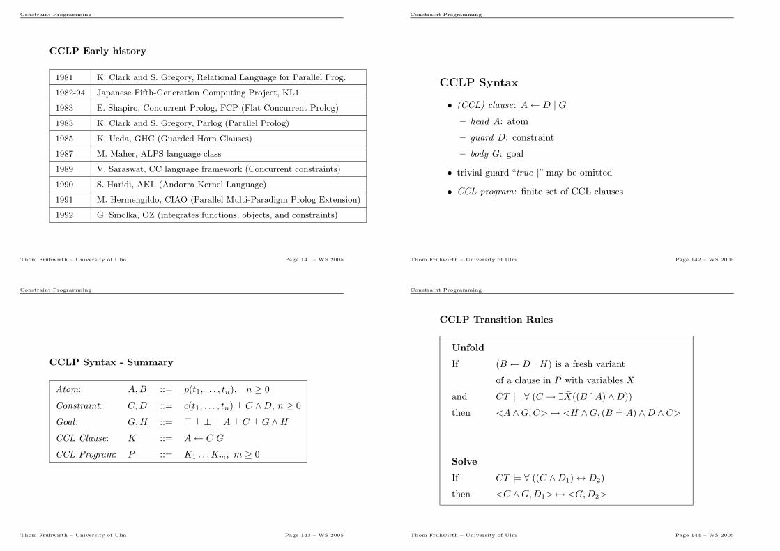
Constraint Programming
CCLP Syntax
• (CCL) clause: A← D | G– head A: atom
– guard D: constraint
– body G: goal
• trivial guard “true |” may be omitted
• CCL program: finite set of CCL clauses
Thom Fruhwirth – University of Ulm Page 142 – WS 2005
Constraint Programming
CCLP Syntax - Summary
Atom: A,B ::= p(t1, . . . , tn), n ≥ 0
Constraint: C,D ::= c(t1, . . . , tn) C ∧D, n ≥ 0
Goal : G,H ::= ⊤ ⊥ A C G ∧HCCL Clause: K ::= A← C|GCCL Program: P ::= K1 . . .Km, m ≥ 0
Thom Fruhwirth – University of Ulm Page 143 – WS 2005
Constraint Programming
CCLP Transition Rules
Unfold
If (B ← D | H) is a fresh variant
of a clause in P with variables X
and CT |= ∀ (C → ∃X((B.=A) ∧D))
then <A ∧G,C> 7→ <H ∧G, (B .= A) ∧D ∧ C>
Solve
If CT |= ∀ ((C ∧D1)↔ D2)
then <C ∧G,D1> 7→ <G,D2>
Thom Fruhwirth – University of Ulm Page 144 – WS 2005
Constraint Programming
CCLP Unfold
If (B ← D | H) is a fresh variant
of a clause in P with variables X
and CT |= ∀ (C → ∃X((B.=A) ∧D))
then <A ∧G,C> 7→ <H ∧G, (B .= A) ∧D ∧ C>
• entailment test/ask : checks implication of guard D by store C,
i.e., CT |= ∀ (C → D)
• clause with head B and guard D is applicable to A in the context
of constraints C, when CT |= ∀(C → ∃X((B=A) ∧D)) holds
• clause application: A removed, body H added to goal store,
equation B=A and guard D added to constraint store (tell)
• committed choice of a clause, cannot be undone
• implicit concurrency (atom selection)Thom Fruhwirth – University of Ulm Page 145 – WS 2005
Constraint Programming
CCLP Unfold – Matching/One-sided Unification
Clause Applicability Condition in Unfold transition rule
CT |= ∀(C → ∃X((B=A) ∧D))
Given the constraints of C, try to solve the constraints (B=A ∧D)
without further constraining (touching) any variable in A and C
• first check that A matches B
– A is an instance of B
– only allowed to instantiate variables from the clause X of B
but not variables of A
• then check the guard D under this matching
((B=A): shorthand for equating arguments of B and A)
Thom Fruhwirth – University of Ulm Page 146 – WS 2005
Constraint Programming
CCLP Example – Matching
CT |= ∀(C → ∃X((B=A) ∧D))
Matching B=A,C = true, D = true
• ∃X(p(X)=p(a))
• ∀Y ∃X(p(X)=p(Y ))
but not
• ∀Y ∃X(p(a)=p(Y ))
More Examples
• CT |= ∀Y (Y =a→ ∃X(p(X)=p(Y )) ∧X=a)
• CT |= ∀Y (Y =a→ (p(a)=p(Y )))
• CT 6|= ∀Y, Z(Z=a→ (p(a)=p(Y )))
Thom Fruhwirth – University of Ulm Page 147 – WS 2005
Constraint Programming
CCLP Deadlock
Successful and failed derivations and goals as in CLP. But new final
state deadlocked.
<G,C> with G different from ⊤ and C different from false and no
more transitions are possible
• consequence of having no Failure transition
• usually programming errors
Thom Fruhwirth – University of Ulm Page 148 – WS 2005
Constraint Programming
CCLP Example – Flipping Coins
flip(Side) ← Side.=face1
flip(Side) ← Side.=face2
• CLP:
flip(Coin) with two answers
• CCLP:
output not predictable: depending on selected clause
e.g., flip(face1) can either be failed or successful
Thom Fruhwirth – University of Ulm Page 149 – WS 2005
Constraint Programming
CCLP Example – Min
min(X,Y,Z) ← X≤Y | X .=Z (c1)
min(X,Y,Z) ← Y≤X | Y .=Z (c2)
• input/output parameters (generalized, per rule)
• For goal min(1,2,C) rule c1 is applicable since
CT |= ∀(true→ ∃ X, Y, Z((1 .=X ∧ 2 .=Y ∧ C .=Z) ∧ X ≤ Y))
Derivation:
<min(1, 2, C), true>
7→Unfold (c1) 〈X .=Z, 1.=X∧2 .=Y∧C .=Z〉
7→Solve 〈⊤, C .=1〉
Thom Fruhwirth – University of Ulm Page 150 – WS 2005
Constraint Programming
CCLP Example – Min (cont)
min(X,Y,Z) ← X≤Y | X .=Z (c1)
min(X,Y,Z) ← Y≤X | Y .=Z (c2)
• <min(A, 2, 1), true>, min(A,2,2), and min(A,2,3) deadlocked
(completely solved in CLP, but with both CL clauses)
• min(A, B, C) ∧ A≤B leads to A≤B ∧ A .=C by selecting the first clause
(compared two answers in CLP, second one was A.=B ∧ A .=C)
Thom Fruhwirth – University of Ulm Page 151 – WS 2005
Constraint Programming
CCLP Example – Hamming
Hamming’s Problem: compute ordered ascending sequence of all
numbers whose only prime factors are 2, 3, or 5:
1 ⋄ 2 ⋄ 3 ⋄ 4 ⋄ 5 ⋄ 6 ⋄ 8 ⋄ 9 ⋄ 10 ⋄ 12 ⋄ 15 ⋄ 16 ⋄ 18 ⋄ 20 ⋄ 24 ⋄ 25 ⋄ ...
• hamming(S) with infinite sequence S
• pretend (infinite!) sequence S is already known
(actually only start 1 is known)
• mults processes multiply the numbers in S with 2, 3, and 5
• merge processes combine results to (ordered, duplicate-free)
sequence S
Thom Fruhwirth – University of Ulm Page 152 – WS 2005
Constraint Programming
CCLP Example – Hamming (cont)
hamming(S) ←S=1⋄S1 ∧mults(S,2,S2) ∧ mults(S,3,S3) ∧ mults(S,5,S5) ∧merge(S2,S3,S23) ∧ merge(S5,S23,S1)
mults(X⋄S,N,XSN) ← XSN=X*N⋄SN ∧ mults(S,N,SN)
merge(X⋄In1,Y⋄In2,XYOut) ← X=Y |XYOut
.=X⋄Out ∧ merge(In1,In2,Out)
merge(X⋄In1,Y⋄In2,XYOut) ← X<Y |XYOut
.=X⋄Out ∧ merge(In1,Y⋄In2,Out)
merge(X⋄In1,Y⋄In2,XYOut) ← X>Y |XYOut
.=Y⋄Out ∧ merge(X⋄In1,In2,Out)
Thom Fruhwirth – University of Ulm Page 153 – WS 2005
Constraint Programming
CCLP Example – Hamming (cont)
• no base cases in recursion as sequences are infinite
• concurrent-process network, processes can be executed in parallel
• mults and merge processes synchronize themselves
• processes communicate via the shared sequence variables
Thom Fruhwirth – University of Ulm Page 154 – WS 2005
Constraint Programming
CCLP Example – Hamming (cont)
Goal hamming(S)
mults(1⋄S1,2,S2) with Unfold and Solve leads to
S2.=2⋄S2N ∧ mults(S1,2,S2N).
Overall, the three mults processes yield
S2.=2⋄S2N ∧ S3
.=3⋄S3N ∧ S5
.=5⋄S5N ∧ mults(S1,2,S2N) ∧
mults(S1,3,S3N) ∧ mults(S1,5,S5N) ∧ merge(S2,S3,S23) ∧merge(S5,S23,S1).
merge(S2,S3,S23) can unfold with the second clause
S23.=2⋄S23N ∧ merge(S2N,S3,S23N).
merge(S5,S23,S1) yields
S1.=2⋄SN ∧ merge(S5,S23N,SN).
Thom Fruhwirth – University of Ulm Page 155 – WS 2005
Constraint Programming
CCLP with Atomic Tell
• eventual tell : constraints occurring in body are added without
consistency check, danger of failure due to Solve
• atomic tell : constraints are added only if they are consistent
together with the current constraint store
Extended CCLP syntax of clauses
CCL Clause K ::= A← C : D G
CCL clause can only Unfold if adding constraint D keeps constraint
store consistent
Thom Fruhwirth – University of Ulm Page 156 – WS 2005
Constraint Programming
CCLP Transition Rules extended with Atomic Tell
Unfold
If (B ← D1 : D2 | H) is a fresh variant of a clause in P
and CT |= ∀ (C → ∃X((B.=A) ∧D1))
and CT |= ∃((B .=A) ∧D1 ∧D2 ∧ C)
Then <A ∧G,C> 7→ <H ∧G, (B .=A) ∧D1 ∧D2 ∧ C>
Solve
If CT |= (C ∧D1)↔ D2
Then <C ∧G,D1> 7→ <G,D2>
Thom Fruhwirth – University of Ulm Page 157 – WS 2005
Constraint Programming
CCLP Atomic Tell Example – Min
Eventual tell
min(X,Y,Z) ← X≤Y | X .=Z
min(X,Y,Z) ← Y≤X | Y .=Z
min(1,2,3) fails
Atomic tell
min(X,Y,Z) ← X≤Y : X=Z | truemin(X,Y,Z) ← Y≤X : Y=Z | true
min(1,2,3) deadlocked
Thom Fruhwirth – University of Ulm Page 158 – WS 2005
Constraint Programming
CCLP Stability
If
• <G,C> 7→Unfold <G′, C′>
• D constraint
• C′ ∧D satisfiable
then also <G ∧H,C ∧D> 7→Unfold <G′ ∧H,C ′ ∧D>.
Thom Fruhwirth – University of Ulm Page 159 – WS 2005
Constraint Programming
CCLP without Atomic Tell Monotonicity
If
• <G,C> 7→Unfold <G′, C′>
• D constraint
• C ∧D satisfiable
then also <G ∧H,C ∧D> 7→Unfold <G′ ∧H,C ′ ∧D>.
The difference between stability and monotonicity is in C ′ ∧D versus
C ∧D.
Thom Fruhwirth – University of Ulm Page 160 – WS 2005
Constraint Programming
CCLP Declarative Semantics
• declarative semantics of CCL programs analogous to that of CL
programs
• symbols “|” and “:” interpreted as conjunctions:
A← C : D | G corresponds to A← C ∧D ∧G
• Clark’s completion of a CCL program is as in CLP
• discrepancy between operational and declarative semantics, as
CCLP goals have only one derivation (compared to CLP goals)
Thom Fruhwirth – University of Ulm Page 161 – WS 2005
Constraint Programming
Soundness of successful derivations
• If G has a successful derivation with an answer constraint C,
then P↔ ∪ CT |= ∀(C → G).
• Analogous to soundness for CL programs.
(P CCL program, G goal)
Thom Fruhwirth – University of Ulm Page 162 – WS 2005
Constraint Programming
CCLP Example – Completeness/Flip Coin
flip(Side) ← Side.=face1
flip(Side) ← Side.=face2
Declarative semantics P↔:
flip(Coin) ⇔ Coin = face1 ∨ Coin = face2
• P↔, CT |= (Coin=face1→ flip(Coin))
• If flip(Coin) has successful derivation with answer constraint C ′
then
CT |= ∀(Coin=face1→ C ′)
• If C ′ = Coin=face2 then
CT 6|= ∀(Coin=face1→ Coin=face2)
Thom Fruhwirth – University of Ulm Page 163 – WS 2005
Constraint Programming
Deterministic CCLP program
• (heads and) guards of a clause exclude each other
• all derivations are the same (up to reordering of reductions due
to stability) and have the same answer constraint
Examples
• min(X,Y,Z) ← X≤Y | X=Z
min(X,Y,Z) ← Y<X | Y=Z
Now <min(A, B, C), A≥B> is deadlocked (due to strict less in
second clause)
• all predicates of Hamming are deterministic
Thom Fruhwirth – University of Ulm Page 164 – WS 2005
Constraint Programming
Completeness of successful derivations
If
• P deterministic CCL program
• G goal with at least one fair derivation, not deadlocked
• P↔ ∪ CT |= ∀ (C → G)
• C is consistent in CT
then each successful derivation of G has an answer constraint C ′ s.t.
CT |= ∀ (C → C ′).
Thom Fruhwirth – University of Ulm Page 165 – WS 2005
Constraint Programming
CCLP Example – Completeness
min(X,Y,Z) ← X ≤ Y | X = Z
min(X,Y,Z) ← Y < X | Y = Z
• goal G = min(A,B,C)
• P↔, CT |= (A ≤ B ∧ A=C→ G)
• initial state <G, true> deadlocked
Therefore no fair derivation.
Thom Fruhwirth – University of Ulm Page 166 – WS 2005
Constraint Programming
Soundness and Completeness of failed derivations
If
• P deterministic CCL program
• G goal with at least one fair derivation, not deadlocked
then the following statements are equivalent
• P↔ ∪ CT |= ¬∃G
• G has a finitely failed derivation
• Each fair derivation of G fails finitely
Thom Fruhwirth – University of Ulm Page 167 – WS 2005
Constraint Programming
Constraint Handling Rules (CHRs)
• constraints often heterogeneous and application specific
• in the beginning “hard-wired” in built-in constraint solver
– efficient (written in low-level language)
– hard to:
∗ modify a solver
∗ build a solver over a new domain
∗ reason about and analyze
∗ debug constraint-based programs
– behavior of solver can neither be inspected by user nor
explained by computer
Thom Fruhwirth – University of Ulm Page 168 – WS 2005
Constraint Programming
CHR – Vision
• CHR constraint language originally designed for writing
constraint solvers
– concurrent committed-choice language
– multi-headed rules that transform constraints into simpler
ones until they are solved
• simplification of and propagation over user-defined constraints
• Simplification replaces constraints by simpler constraints while
preserving logical equivalence, e.g. (where “leq” is the constraint
for “≤”): X leq Y ∧ Y leq X ⇔ X=Y.
• Propagation adds new constraints, which are logically redundant
but may cause further simplification, e.g.,
X leq Y ∧ Y leq Z ⇒ X leq Z.
Thom Fruhwirth – University of Ulm Page 169 – WS 2005
Constraint Programming
CHR – Applications
• theorem proving and computational logic
– forward and backward chaining
– (integrity) constraints
– tabulation
– abduction
– deduction
• as general-purpose concurrent constraint language
• as flexible production rule system with constraints
Thom Fruhwirth – University of Ulm Page 170 – WS 2005
Constraint Programming
CHR – Available Distributions
About 10 implementations
• Prolog: SICStus, Yap, Eclipse, XSB, hProlog, HAL, SWI
• Java (3)
• Haskell (2)
Thom Fruhwirth – University of Ulm Page 171 – WS 2005
Constraint Programming
CHR Syntax
• generalization of CCLP calculus
• disjoint sets of predicate symbols
– (built-in) constraint symbols
– (user-defined) CHR constraint symbols
• built-in constraints handled by predefined given constraint solvers
• CHR constraints are defined by a CHR program
Thom Fruhwirth – University of Ulm Page 172 – WS 2005
Constraint Programming
CHR Syntax (2)
Simplification rule: E ⇔ C G
Propagation Rule: E ⇒ C G
• head E: CHR constraint
• guard C: built-in constraint
• body G: goal, i.e.,
– ⊤ or ⊥, or
– built-in constraint or CHR constraint, or
– conjunction of goals
• CHR program: finite set of rules
• CHR constraint symbol defined : it occurs in the head of a rule
• trivial guard “ true ” can be omitted
Thom Fruhwirth – University of Ulm Page 173 – WS 2005
Constraint Programming
CHR Syntax – Summary
Built-in Constraint : C,D ::= c(t1, . . . , tn) C ∧D, n ≥ 0
CHR Constraint : E,F ::= e(t1, . . . , tn) E ∧ F , n ≥ 0
Goal : G,H ::= ⊤ ⊥ C E G ∧HCHR Rule: R ::= E ⇔ C | G E ⇒ C | GCHR Program: P ::= R1 . . . Rm,m ≥ 0
Thom Fruhwirth – University of Ulm Page 174 – WS 2005
Constraint Programming
CHR Operational Semantics
• state <G,C>: G goal (store), C (built-in) constraint (store)
• initial state <G, true>
• successful final state <E,C>:
no transition is applicable, C is different from false
• failed final state <G, false>
CCLP deadlocked states vs. CHR successful states
• CHR constraints that could not be further simplified
• do not imply consistency of logical reading
Thom Fruhwirth – University of Ulm Page 175 – WS 2005
Constraint Programming
CHR Transition Rules
• Simplify (extends Unfold of CCLP)
• Propagate (similar Simplify)
• Solve (as in CCLP)
Thom Fruhwirth – University of Ulm Page 176 – WS 2005
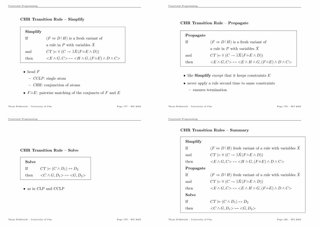
Constraint Programming
CHR Transition Rule – Simplify
Simplify
If (F ⇔ D H) is a fresh variant of
a rule in P with variables X
and CT |= ∀ (C → ∃X(F =E ∧D))
then <E ∧G,C> 7→ <H ∧G, (F =E) ∧D ∧ C>
• head F
– CCLP: single atom
– CHR: conjunction of atoms
• F =E: pairwise matching of the conjuncts of F and E
Thom Fruhwirth – University of Ulm Page 177 – WS 2005
Constraint Programming
CHR Transition Rule – Propagate
Propagate
If (F ⇒ D H) is a fresh variant of
a rule in P with variables X
and CT |= ∀ (C → ∃X(F =E ∧D))
then <E ∧G,C> 7→ <E ∧H ∧G, (F =E) ∧D ∧ C>
• like Simplify except that it keeps constraints E
• never apply a rule second time to same constraints
– ensures termination
Thom Fruhwirth – University of Ulm Page 178 – WS 2005
Constraint Programming
CHR Transition Rule – Solve
Solve
If CT |= (C ∧D1)↔ D2
then <C ∧G,D1> 7→ <G,D2>
• as in CLP and CCLP
Thom Fruhwirth – University of Ulm Page 179 – WS 2005
Constraint Programming
CHR Transition Rules – Summary
Simplify
If (F ⇔ D H) fresh variant of a rule with variables X
and CT |= ∀ (C → ∃X(F =E ∧D))
then <E ∧G,C> 7→ <H ∧G, (F =E) ∧D ∧ C>Propagate
If (F ⇒ D H) fresh variant of a rule with variables X
and CT |= ∀ (C → ∃X(F =E ∧D))
then <E ∧G,C> 7→ <E ∧H ∧G, (F =E) ∧D ∧ C>Solve
If CT |= (C ∧D1)↔ D2
then <C ∧G,D1> 7→ <G,D2>
Thom Fruhwirth – University of Ulm Page 180 – WS 2005
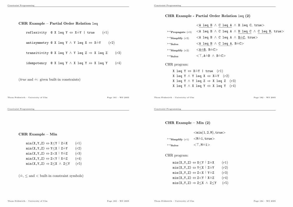
Constraint Programming
CHR Example – Partial Order Relation leq
reflexivity @ X leq Y ⇔ X=Y | true (r1)
antisymmetry @ X leq Y ∧ Y leq X ⇔ X=Y (r2)
transitivity @ X leq Y ∧ Y leq Z ⇒ X leq Z (r3)
idempotency @ X leq Y ∧ X leq Y ⇔ X leq Y (r4)
(true and.=: given built-in constraints)
Thom Fruhwirth – University of Ulm Page 181 – WS 2005
Constraint Programming
CHR Example - Partial Order Relation leq (2)
<A leq B ∧ C leq A ∧ B leq C, true>
7→Propagate (r3) <A leq B ∧ C leq A ∧ B leq C ∧ C leq B, true>
7→Simplify (r2) <A leq B ∧ C leq A ∧ B=C, true>
7→Solve <A leq B ∧ C leq A, B=C>
7→Simplify (r2) <A=B, B=C>
7→Solve <⊤, A=B ∧ B=C>
CHR program:
X leq Y ⇔ X=Y | true (r1)
X leq Y ∧ Y leq X ⇔ X=Y (r2)
X leq Y ∧ Y leq Z ⇒ X leq Z (r3)
X leq Y ∧ X leq Y ⇔ X leq Y (r4)
Thom Fruhwirth – University of Ulm Page 182 – WS 2005
Constraint Programming
CHR Example – Min
min(X,Y,Z)⇔ X≤Y Z=X (r1)
min(X,Y,Z)⇔ Y≤X Z=Y (r2)
min(X,Y,Z)⇔ Z<X Y=Z (r3)
min(X,Y,Z)⇔ Z<Y X=Z (r4)
min(X,Y,Z)⇒ Z≤X ∧ Z≤Y (r5)
(=, ≤ and < built-in constraint symbols)
Thom Fruhwirth – University of Ulm Page 183 – WS 2005
Constraint Programming
CHR Example – Min (2)
<min(1, 2, M), true>
7→Simplify (r1) <M=1, true>
7→Solve <⊤, M=1>
CHR program:
min(X,Y,Z)⇔ X≤Y Z=X (r1)
min(X,Y,Z)⇔ Y≤X Z=Y (r2)
min(X,Y,Z)⇔ Z<X Y=Z (r3)
min(X,Y,Z)⇔ Z<Y X=Z (r4)
min(X,Y,Z)⇒ Z≤X ∧ Z≤Y (r5)
Thom Fruhwirth – University of Ulm Page 184 – WS 2005
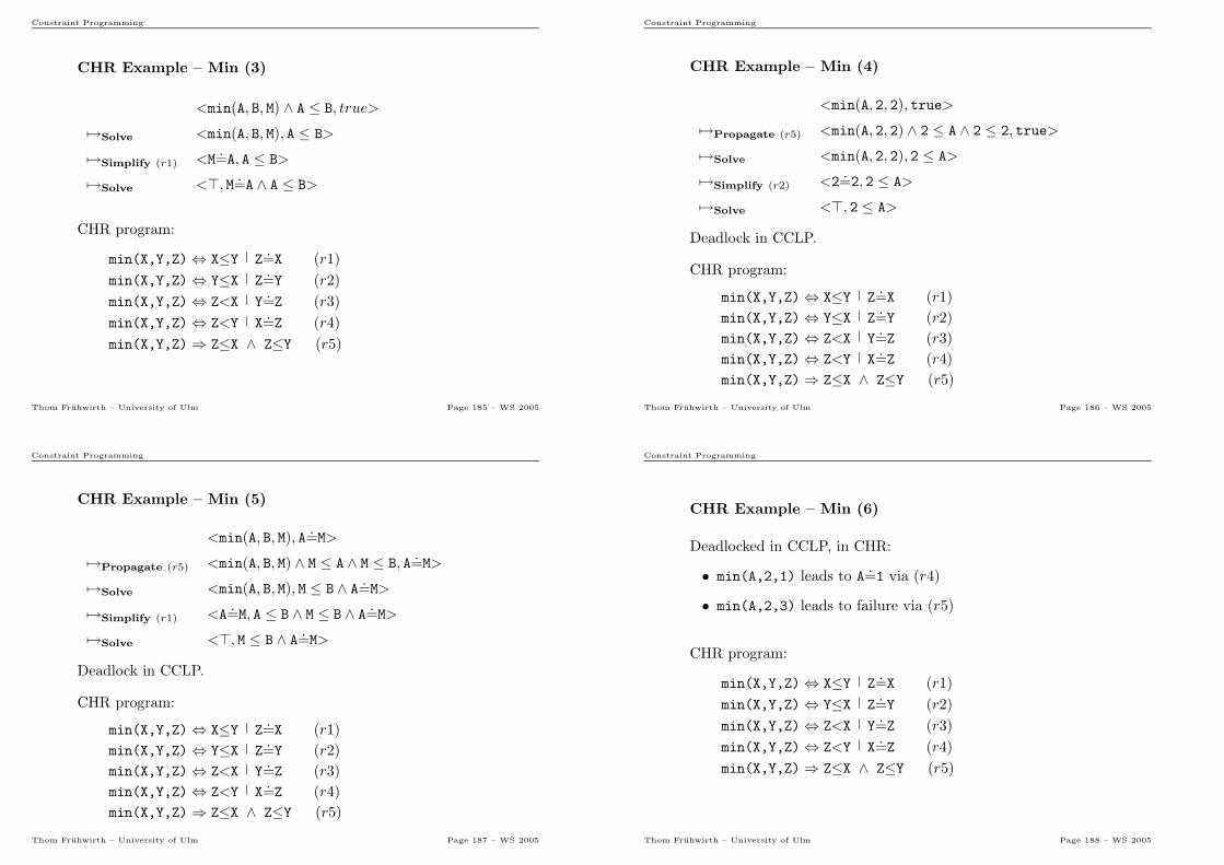
Constraint Programming
CHR Example – Min (3)
<min(A, B, M) ∧ A ≤ B, true>
7→Solve <min(A, B, M), A ≤ B>
7→Simplify (r1) <M=A, A ≤ B>
7→Solve <⊤, M=A ∧ A ≤ B>
CHR program:
min(X,Y,Z)⇔ X≤Y Z=X (r1)
min(X,Y,Z)⇔ Y≤X Z=Y (r2)
min(X,Y,Z)⇔ Z<X Y=Z (r3)
min(X,Y,Z)⇔ Z<Y X=Z (r4)
min(X,Y,Z)⇒ Z≤X ∧ Z≤Y (r5)
Thom Fruhwirth – University of Ulm Page 185 – WS 2005
Constraint Programming
CHR Example – Min (4)
<min(A, 2, 2), true>
7→Propagate (r5) <min(A, 2, 2) ∧ 2 ≤ A ∧ 2 ≤ 2, true>
7→Solve <min(A, 2, 2), 2 ≤ A>
7→Simplify (r2) <2=2, 2 ≤ A>
7→Solve <⊤, 2 ≤ A>
Deadlock in CCLP.
CHR program:
min(X,Y,Z)⇔ X≤Y Z=X (r1)
min(X,Y,Z)⇔ Y≤X Z=Y (r2)
min(X,Y,Z)⇔ Z<X Y=Z (r3)
min(X,Y,Z)⇔ Z<Y X=Z (r4)
min(X,Y,Z)⇒ Z≤X ∧ Z≤Y (r5)
Thom Fruhwirth – University of Ulm Page 186 – WS 2005
Constraint Programming
CHR Example – Min (5)
<min(A, B, M), A=M>
7→Propagate (r5) <min(A, B, M) ∧ M ≤ A ∧ M ≤ B, A=M>
7→Solve <min(A, B, M), M ≤ B ∧ A=M>
7→Simplify (r1) <A=M, A ≤ B ∧ M ≤ B ∧ A=M>
7→Solve <⊤, M ≤ B ∧ A=M>
Deadlock in CCLP.
CHR program:
min(X,Y,Z)⇔ X≤Y Z=X (r1)
min(X,Y,Z)⇔ Y≤X Z=Y (r2)
min(X,Y,Z)⇔ Z<X Y=Z (r3)
min(X,Y,Z)⇔ Z<Y X=Z (r4)
min(X,Y,Z)⇒ Z≤X ∧ Z≤Y (r5)
Thom Fruhwirth – University of Ulm Page 187 – WS 2005
Constraint Programming
CHR Example – Min (6)
Deadlocked in CCLP, in CHR:
• min(A,2,1) leads to A=1 via (r4)
• min(A,2,3) leads to failure via (r5)
CHR program:
min(X,Y,Z)⇔ X≤Y Z=X (r1)
min(X,Y,Z)⇔ Y≤X Z=Y (r2)
min(X,Y,Z)⇔ Z<X Y=Z (r3)
min(X,Y,Z)⇔ Z<Y X=Z (r4)
min(X,Y,Z)⇒ Z≤X ∧ Z≤Y (r5)
Thom Fruhwirth – University of Ulm Page 188 – WS 2005
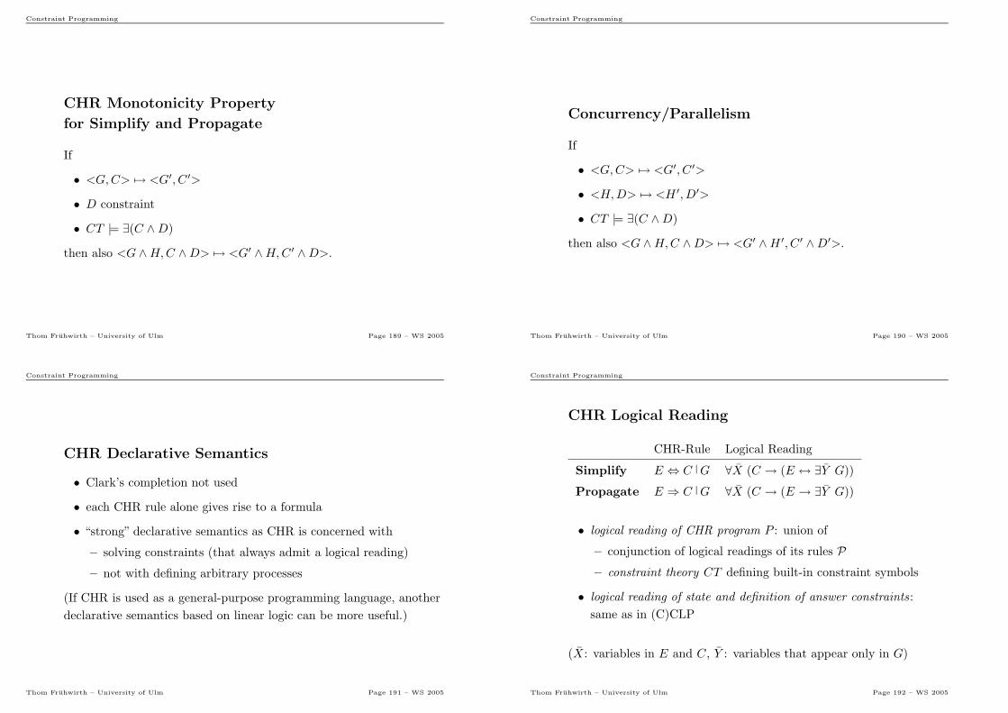
Constraint Programming
CHR Monotonicity Property
for Simplify and Propagate
If
• <G,C> 7→ <G′, C′>
• D constraint
• CT |= ∃(C ∧D)
then also <G ∧H,C ∧D> 7→ <G′ ∧H,C ′ ∧D>.
Thom Fruhwirth – University of Ulm Page 189 – WS 2005
Constraint Programming
Concurrency/Parallelism
If
• <G,C> 7→ <G′, C′>
• <H,D> 7→ <H ′, D′>
• CT |= ∃(C ∧D)
then also <G ∧H,C ∧D> 7→ <G′ ∧H ′, C′ ∧D′>.
Thom Fruhwirth – University of Ulm Page 190 – WS 2005
Constraint Programming
CHR Declarative Semantics
• Clark’s completion not used
• each CHR rule alone gives rise to a formula
• “strong” declarative semantics as CHR is concerned with
– solving constraints (that always admit a logical reading)
– not with defining arbitrary processes
(If CHR is used as a general-purpose programming language, another
declarative semantics based on linear logic can be more useful.)
Thom Fruhwirth – University of Ulm Page 191 – WS 2005
Constraint Programming
CHR Logical Reading
CHR-Rule Logical Reading
Simplify E ⇔ C G ∀X (C → (E ↔ ∃Y G))
Propagate E ⇒ C G ∀X (C → (E → ∃Y G))
• logical reading of CHR program P : union of
– conjunction of logical readings of its rules P– constraint theory CT defining built-in constraint symbols
• logical reading of state and definition of answer constraints:
same as in (C)CLP
(X: variables in E and C, Y : variables that appear only in G)
Thom Fruhwirth – University of Ulm Page 192 – WS 2005
Constraint Programming
CHR Soundness and Completeness
Equivalence of States
• computable constraint of G: logical reading of a state which
appears in a derivation of G
• for all computable constraints C1 and C2 of G:
P ∪ CT |= ∀ (C1 ↔ C2)
• no distinction between successful and failed derivations
(P : CHR program, G: goal)
Thom Fruhwirth – University of Ulm Page 193 – WS 2005
Constraint Programming
CHR Soundness
If
• G has a derivation with answer constraint C
then P ∪ CT |= ∀ (C ↔ G).
(P : CHR program, G: goal)
Thom Fruhwirth – University of Ulm Page 194 – WS 2005
Constraint Programming
CHR Completeness
If
• G with at least one finite derivation
• P ∪ CT |= ∀ (C ↔ G)
then
• G has a derivation with answer constraint C ′
• P ∪ CT |= ∀ (C ↔ C ′).
(P : CHR program, G: goal)
Thom Fruhwirth – University of Ulm Page 195 – WS 2005
Constraint Programming
CHR Example – Completeness
CHR program P :
p⇔ p
CHR Completeness does not hold if G has no finite derivation
• goal G: p
• P ∪ CT |= p↔ p
• but G has only one infinite derivation
Thom Fruhwirth – University of Ulm Page 196 – WS 2005
Constraint Programming
CHR Soundness and Completeness for Failed
Derivations
If goal G has a finitely failed derivation, then P ∪ CT |= ¬∃G.
But the converse does not hold, e.g.
p ⇔ q
p ⇔ false
• P ∪ CT |= ¬q
• q has no finitely failed derivation, but a successful one
Thom Fruhwirth – University of Ulm Page 197 – WS 2005
Constraint Programming
CHR Confluence – Motivation
Result of a derivation of a given goal will always have the same
meaning.
Without confluence:
• not guaranteed that the result is syntactically the same
• a solver may be able to detect inconsistency of constraints with
one order of rule applications but not with another
With confluence:
• guaranteed that result is syntactically the same
Confluence generalizes the notion of deterministic CCLP.
Thom Fruhwirth – University of Ulm Page 198 – WS 2005
Constraint Programming
CHR Confluence
The answer of a query is always the same, no matter which of the
applicable rules are applied.
• confluent : for all states S, S1, and S2
If S 7→∗ S1 and S 7→∗ S2 then S1 and S2 are joinable.
• joinable: if there exist states T1 and T2 such that S1 7→∗ T1 and
S2 7→∗ T2 and T1 and T2 are variants.
In general infinitely many states to test.
Thom Fruhwirth – University of Ulm Page 199 – WS 2005
Constraint Programming
CHR Confluence with Terminating Programs
• terminating CHR program: there are no infinite derivations
• decidable, sufficient, and necessary condition for confluence
A terminating CHR program is confluent if and only if all its critical
pairs are joinable.
Thom Fruhwirth – University of Ulm Page 200 – WS 2005
Constraint Programming
CHR Confluence Test
Critical Ancestor State of R1 and R2
<H1 ∧A1 ∧H2, (A1=A2) ∧ C1 ∧ C2>
• (R1) H1 ∧A1 ⇔ C1 G1: simplification rule
• (R2) H2 ∧A2
⇔⇒
C2 G2: rule with variables renamed apart
• A1 and A2: non-empty conjunctions
• CT |= ∃((A1=A2) ∧ C1 ∧ C2)
Thom Fruhwirth – University of Ulm Page 201 – WS 2005
Constraint Programming
CHR Confluence Test (2)
Critical Pair (S1, S2)
• S: critical ancestor state of R1 and R2
• S 7→R1 S1, S 7→R2 S2
• check join-ability
– S1 7→∗ T1, S2 7→∗ T2
– T1, T2 variants?
Thom Fruhwirth – University of Ulm Page 202 – WS 2005
Constraint Programming
CHR Example – Confluence for leq
X leq Y ⇔ X=Y | true (r1)
X leq Y ∧ Y leq X ⇔ X=Y (r2)
X leq Y ∧ Y leq Z ⇒ X leq Z (r3)
X leq Y ∧ X leq Y ⇔ X leq Y (r4)
• <X leq Y ∧ Y leq X ∧ Y leq Z, true>
critical ancestor state of (r2) and (r3)
• (S1, S2) =
(<X=Y ∧ Y leq Z, true>,
<X leq Y ∧ Y leq X ∧ Y leq Z ∧ X leq Z, true>)
critical pair is joinable
Thom Fruhwirth – University of Ulm Page 203 – WS 2005
Constraint Programming
CHR Example – Confluence for leq (2)
A derivation beginning with S1 proceeds as follows:
<X=Y ∧ Y leq Z, true>
7→Solve < Y leq Z, X=Y>
A derivation beginning with S2 results in the same final state:
<X leq Y ∧ Y leq X ∧ Y leq Z ∧ X leq Z, true>
7→Simplify (r2) <X=Y ∧ Y leq Z ∧ X leq Z, true>
7→Solve <Y leq Z ∧ X leq Z, X=Y>
7→Simplify (r4) <Y leq Z, X=Y>
Thom Fruhwirth – University of Ulm Page 204 – WS 2005
Constraint Programming
CHR Soundness and Completeness of Failed
Derivations
If
• P : terminating and confluent CHR program
• G: goal with at least one answer constraint consisting of only
built-in constraints
then
P ∪ CT |= ¬∃G if and only if each finite derivation starting with
<G, true> fails.
Thom Fruhwirth – University of Ulm Page 205 – WS 2005
Constraint Programming
CHR Example – Confluence Coin
flip(Coin) ⇔ true | Coin = face1,
flip(Coin) ⇔ true | Coin = face2
The source state
<flip(Coin), true>
yields the following target states (forming a critical pair):
<Coin=face1,⊤> versus <Coin=face2,⊤>
These two states are not joinable, hence the program is not confluent.
Thom Fruhwirth – University of Ulm Page 206 – WS 2005
Constraint Programming
CHR Example – Confluence Min
min(X,Y,Z) ⇔ X ≤ Y | X = Z,
min(X,Y,Z) ⇔ Y ≤ X | Y = Z
Overlapping the two rules yields the source state
<min(X, Y, Z), X ≤ Y ∧ Y ≤ X>
and the critical pair
<X=Z,X ≤ Y ∧ Y ≤ X> versus <Y =Z,X ≤ Y ∧ Y ≤ X>
Both states of the critical pair can yield
<⊤, X=Y ∧ Y =Z>
Hence the program is confluent.
Thom Fruhwirth – University of Ulm Page 207 – WS 2005
Constraint Programming
CHR∨: Adding Disjunction
• CHR originally intended as declarative language for rapid
prototyping and efficient implementation of constraint solvers
– concurrent committed-choice language
– lacks the don’t-know non-determinism of CLP
• subsume the expressive power of CLP: disjunctions on the
right-hand sides of CHR rules
• entire application in a uniform language
Thom Fruhwirth – University of Ulm Page 208 – WS 2005
Constraint Programming
CHR∨Split
Split
<(H1 ∨H2) ∧G,C> 7→ <H1 ∧G,C> | <H2 ∧G,C>
• additional transition Split for CHR∨, to deal with disjunction ∨
• similar to UnfoldSplit rule in CLP
Example:
min(X,Y ,Z) <=> true | ((X ≤ Y ∧X=Z) ∨ (Y ≤ X ∧ Y =Z))
Thom Fruhwirth – University of Ulm Page 209 – WS 2005
Constraint Programming
Constraint System (Σ,D, CT, C)• signature Σ: contains constraint symbols, at least
– true/0 and false/0, and
– syntactic equality =/2
• domain (universe) D together with interpretation of function and
constraint symbols in Σ
• constraint theory CT over Σ:
– non-empty
– consistent
• allowed constraints C:– all constraints from Σ
– closed under existential quantification (or: variable renaming)
and conjunction
Thom Fruhwirth – University of Ulm Page 210 – WS 2005
Constraint Programming
Constraint System E (Syntactic Equality)
• signature Σ: contains
– countably infinitely many function symbols, including at least
one constant
– constraint symbols true/0, false/0, and =/2
• domain D: Herbrand universe
• constraint theory CT : CET (Clark’s Equality Theory)
• allowed constraints
C ::= true false s=t ∃x C C ∧ C
(s, t: terms over Σ)
Thom Fruhwirth – University of Ulm Page 211 – WS 2005
Constraint Programming
Constraint Theory
Completeness
For every constraint C, either CT |= C or CT |= ¬C.
Satisfaction-completeness
For every allowed constraint C ∈ C, either CT |= ∃C or CT |= ¬∃C.
Example:
• CET is complete
• If there were only finitely many function symbols in Σ
– not complete
– but satisfaction-complete
Thom Fruhwirth – University of Ulm Page 212 – WS 2005
Constraint Programming
Independence of Negated Constraints (INC)
For all constraints C,C1, . . . , Cn ∈ C
CT |= ∃(C ∧ ¬C1 ∧ . . . ∧ ¬Cn) iff CT |= ∃(C ∧ ¬Ci) for i = 1, . . . , n
CT |= ∀(C →∨
i=1,...,n
Ci) iff CT |= ∀(C → Ci) for at least one i
Examples:
• infinite boolean algebras with positive constraints
• linear arithmetic equations over rational or real numbers
• constraint system E: Herbrand terms with infinitely many
function symbols including at least one constant
• feature trees with infinitely many sorts and features
• restricted classes of set constraints (without empty sets)
Not INC: Any constraint system is closed under negation.Thom Fruhwirth – University of Ulm Page 213 – WS 2005
Constraint Programming
Example – Order Relation < over Integers
No independence of negated constraints.
Example:
CT |= ∃(C ∧ ¬Ci) for i = 1, . . . , 3 (given by:)
• CT |= ∃X,Y (true ∧ ¬(X<Y ))
• CT |= ∃X,Y (true ∧ ¬(X=Y ))
• CT |= ∃X,Y (true ∧ ¬(Y <X))
iff CT |= ∃(C ∧ ¬C1¬ ∧ ¬C2 ∧ ¬C3). Therefore:
• CT 6|= ∃X,Y (true ∧ ¬(X<Y ) ∧ ¬(X=Y ) ∧ ¬(Y <X))
Thom Fruhwirth – University of Ulm Page 214 – WS 2005
Constraint Programming
Example – Constraint System E with finite signature
No independence of negated constraints.
Signature of E with only one constant a and one function symbol
f/1.
Example:
• CET ′ |= ∃X,Y (X=f(Y ) ∧ ¬(Y =a))
• CET ′ |= ∃X,Y, Z(X=f(Y ) ∧ ¬(Y =f(Z))).
but
• CET ′ 6|= ∃X,Y, Z(X=f(Y ) ∧ ¬(Y =a) ∧ ¬(Y =f(Z)))
Thom Fruhwirth – University of Ulm Page 215 – WS 2005
Constraint Programming
Example – Constraint System E extended by 6=
No independence of negated constraints.
• 6=: added to Σ
• s 6=t↔ ¬(s=t): added to CT
Example
• CT |= ∃X (true ∧ ¬(X=a))
• CT |= ∃X (true ∧ ¬(X 6=a))
but
• CT 6|= ∃X (true ∧ ¬(X=a) ∧ ¬(X 6=a)).
Thom Fruhwirth – University of Ulm Page 216 – WS 2005
Constraint Programming
Constraint Solvers
• implement algorithms for solving allowed constraints in
accordance with constraint theory
• collect the constraints that arrive incrementally from one or more
running programs
• put constraints into the constraint store
• test satisfiability, simplify, and if possible solve constraints
Thom Fruhwirth – University of Ulm Page 217 – WS 2005
Constraint Programming
Capabilities of Constraint Solvers
As required by constraint programming languages (solve transition
and transition preconditions).
Reasoning Services (in order of importance)
• Satisfiability (Consistency) test
• Simplification
• Variable determination
• Variable projection/elimination
• Entailment test
Thom Fruhwirth – University of Ulm Page 218 – WS 2005
Constraint Programming
Satisfiability (Consistency) test
The solver returns false if C is inconsistent: CT |= ¬∃C.
• solver implements a decision procedure for satisfiability of allowed
constraints
• syntactic equality and linear polynomial equations admit efficient
satisfaction-complete algorithm
• Boolean satisfiability is NP-complete (there is no efficient
algorithm), same for finite domains
Example:
X>X is inconsistent, X>Y is consistent
Thom Fruhwirth – University of Ulm Page 219 – WS 2005
Constraint Programming
Simplification
The solver tries to transform a given constraint C into a logically
equivalent, but simpler constraint D (solve transition):
CT |= ∀(C ↔ D).
• simpler constraint can be handled more efficiently when new
constraints arrive
• improve presentation of answer constraint
• what simpler exactly means depends on the constraint system
(often in the eye of the beholder)
• finding most simple representation can be substantially harder
than solving
Example:
X≤2 ∧X≤4 is simplified into X≤2
2∗X=6 into X=3
Thom Fruhwirth – University of Ulm Page 220 – WS 2005
Constraint Programming
Variable Determination
Detect that a variable X occurring in a constraint C can only take a
unique value: CT |= ∀(C → X=v), where v is a value.
• special case of simplification
• important for representing answer constraints as solutions that
give values to variables
• supports a simple way of communication between different
constraint solvers via shared variables by exchanging values for
those variables
Example:
X≤2 ∧ 2≤X implies X=2
X2=X ∧X < 1 implies X=0
Thom Fruhwirth – University of Ulm Page 221 – WS 2005
Constraint Programming
Variable projection/elimination
Eliminate a variable X by projecting a constraint C onto all other
variables: CT |= ∃XC ↔ D, where D does not contain X .
• keep constraint store small
• simplify answer constraint by eliminating local variables
• but in some cases not possible, significant increase in
size/number for constraints,
Thom Fruhwirth – University of Ulm Page 222 – WS 2005
Constraint Programming
Examples – Variable projection/elimination
• Elimination of Y in
∃Y (X1<Y ∧ . . . ∧Xm<Y ∧ Y <Z1 ∧ . . . ∧ Y <Zn) yields n∗mconstraints of the form Xi<Zj .
• Projection of ∃Y (X<Y ∧ Y <Z) onto X and Z results in X<Z
over the reals and X+1<Z over the integers.
• In the constraint system E, in the formula ∃Y (X=f(Y )), the
variable Y cannot be eliminated
Thom Fruhwirth – University of Ulm Page 223 – WS 2005
Constraint Programming
Entailment test
Check whether a constraint C implies D: CT |= ∀(C → D)?
• required for guard checks in concurrent constraint languages like
CCLP and CHR
• (incomplete) entailment test can be implemented as follows:
if C ∧D simplifies to C, then C → D, or:
if C ∧ ¬D is inconsistent, then C → D.
Thom Fruhwirth – University of Ulm Page 224 – WS 2005
Constraint Programming
Example – Entailment test
X<Y entails X≤Y , but not vice versa.
• X<Y → X≤Y entailed
– solve(X < Y ∧X ≤ Y ) = (X < Y )
– solve(X < Y ∧X > Y ) = false
• X≤Y → X < Y not entailed
– solve(X ≤ Y ∧X < Y ) = (X < Y )
– solve(X ≤ Y ∧X ≥ Y ) = (X = Y )
Thom Fruhwirth – University of Ulm Page 225 – WS 2005
Constraint Programming
Reasoning Services – Implementation
• variations of simplification that maintain a normal form of the
constraints
• implement simplification efficiently – average time complexity
should be a polynomial of low degree
• prefers incomplete implementations if complete one would take
exponential time
Thom Fruhwirth – University of Ulm Page 226 – WS 2005
Constraint Programming
Properties of Constraint Solvers
Constraint solver modeled as a function solve over allowed
constraints.
• Correct : If solve(C) = D, then CT |= ∀(C ↔ D)
• Satisfaction-complete: If CT |= ¬∃C, then solve(C) = false
• Incremental : solve(solve(C) ∧D) = solve(C ∧D)
– ideally, the incremental computation solve(solve(C) ∧D)
should not be more costly than solve(C ∧D)
• Independence of variable naming : C and D are variants of each
other, then solve(C) and solve(D) are variants
Thom Fruhwirth – University of Ulm Page 227 – WS 2005
Constraint Programming
Properties of Constraint Solvers (2)
• Congruence respecting :
Associative solve((C ∧D) ∧ E) = solve(C ∧ (D ∧ E))
Identity solve(C ∧ true) = solve(C)
Commutative solve(C ∧D) = solve(D ∧ C)
• Idempotent : solve(solve(C)) = solve(C)
– solve computes a fixpoint
– no gain in simplifying simplified constraints again
• Canonical : If CT |= ∀(C ↔ D), then solve(C) = solve(D)
– very strong condition, implying all previous ones
Terminating and confluent CHR program is idempotent, congruence
respecting, and incremental.
Thom Fruhwirth – University of Ulm Page 228 – WS 2005
Constraint Programming
Properties of Constraint Solvers (3)
Dependency on Variable Order
Algorithms based on variable elimination (e.g., solving linear
polynomial equations) often rely on an order of variables.
(Typical variable orders: chronological or alphabetical.)
• different variable orders may result in different simplified
constraints, e.g., X=Y vs. Y=X
• properties may not hold anymore
– Independence of variable naming
– Congruence respecting
– Incremental
– Canonical
Thom Fruhwirth – University of Ulm Page 229 – WS 2005
Constraint Programming
Principles of Constraint-Solving Algorithms
• variable-elimination (equation solving)
– satisfaction-complete
• local-consistency (local-propagation)
– interleaved with search to achieve completeness
Thom Fruhwirth – University of Ulm Page 230 – WS 2005
Constraint Programming
Variable Elimination
Allowed constraints are equations.
• e1 = e2
– l.h.s. (left-hand side) e1
– r.h.s. (right-hand side) e2
• normal form: X=e
e expression of some specific syntactic form, e.g. linear
polynomials
• otherwise introduce auxiliary variables, to introduce equalities,
e.g., replace X>Y by X=Y+Z ∧ Z>0
Thom Fruhwirth – University of Ulm Page 231 – WS 2005
Constraint Programming
Variable Elimination (2)
Solved (normal) form or solution: logically equivalent formulation
• determines variables (gives values to variables)
• unique (if possible)
usually
• conjunction of syntactic equality constraints X=v
• X only l.h.s. occurrence of the variable
• v value
Examples:
• X=Y ∧ X=Z not in solved form, X occurs twice on l.h.s.
• X=Y ∧ Y=Z and X=Z ∧ Z=Y in solved form
• Gaussian elimination for solving linear polynomial equations
X=7−Y ∧ X=3+Y leads to X=5 ∧ Y=2Thom Fruhwirth – University of Ulm Page 232 – WS 2005
Constraint Programming
Variable Elimination Algorithms
Eliminate multiple occurrences of variables.
• repeatedly choose an equation X=e, replace all other occurrences
of X by e
• simplify s.t. normal form is maintained
• termination result may rely on order of variables and expressions
• usually not confluent, e.g. X=7−Y−2Z ∧ X=3+Y may lead to
X=3+Y ∧ Y=2−Z or
X=5−Z ∧ Y=2−Z
Thom Fruhwirth – University of Ulm Page 233 – WS 2005
Constraint Programming
Local Consistency (Local Propagation)
Small fixed-size sub-problems of the initial problem considered
repeatedly until a fixpoint is reached.
• sub-problems are simplified and new implied (redundant)
constraints are computed (propagated) from them
• constraints are added hoping that they cause simplification
Examples:
• X>Y ∧ Y >Z ∧ Z>X
the first two constraints imply X>Z and together with Z>X
imply false, i.e., inconsistency is detected (satisfaction complete).
• X 6= Y ∧ Y 6= Z ∧X 6= Z over D = {0, 1} (incomplete for
sub-problems of two constraints) but X 6= Y ∧ Y 6= Z → X = Z.
Thom Fruhwirth – University of Ulm Page 234 – WS 2005
Constraint Programming
Local Consistency (Local Propagation) (2)
Polynomial number of small sub-problems.
• sub-problems in polynomial time then overall algorithm in
polynomial time
• classical consistency algorithms first explored for constraint
networks in artificial intelligence research in the late 1960s.
Originally, the algorithms involved unary and binary constraints
over finite sets of values only.
• arc consistency and path consistency: main classical algorithms
Thom Fruhwirth – University of Ulm Page 235 – WS 2005
Constraint Programming
Local Consistency – Flat Normal Form
Variables are the only arguments of functions.
• often required by local-consistency methods
• flattening : performing the opposite of variable elimination
– replace each non-variable sub-expression by a new variable
– equate this new variable with the sub-expression
• uniform treatment of allowed constraints but introduction of
auxiliary variables
• consistency methods sensitive to representation of constraints,
but no efficient way to find an optimal representation
Examples:
• 2X+Y >5 flattened into W>F ∧ X+V=W ∧ X+Y=V ∧ F=5
• X2>3Y flattened into L>R ∧ L=XT ∧ T=2 ∧ R=DY ∧D = 3
Thom Fruhwirth – University of Ulm Page 236 – WS 2005
Constraint Programming
Search
Local-consistency methods combined with search to achieve
satisfaction-completeness, i.e., global consistency.
• branching: introduce branches in search tree
• case analysis: case splitting by introducing choices
• exponential complexity to combinatorial and other NP-complete
constraint problems, because dependencies between choices are
not and cannot be fully taken care of
• interleaved with constraint solving (repeat until solution is found)
– perform local propagation
– constraint is simplified together with the existing constraints
– search step performed, it adds a new constraint
Thom Fruhwirth – University of Ulm Page 237 – WS 2005
Constraint Programming
Search routines/procedures
Labeling procedure or enumeration procedure (routine): try possible
values for a variable X=v1 ∨ . . . ∨X=vn
• labeling procedure will use heuristics to choose the next variable
and value for labeling
• variable ordering : chosen sequence of variables
first-fail principle: choose the most constrained variable first; will
often lead to failure quickly, thus pruning the search tree early
• value ordering: next value for labeling a variable must be chosen
In the general case, replace a constraint by a logically equivalent
disjunction of constraints, where the disjuncts are pairwise
unsatisfiable (or at least do not imply each other), e.g., X 6=Y can be
expressed as X<Y ∨X>Y .
Thom Fruhwirth – University of Ulm Page 238 – WS 2005
Constraint Programming
Constraint Systems – Preliminaries
• variety of algorithms, mostly adapted from artificial intelligence,
graph theory, and operations research
• CHR∨ used
– Prolog style disjunction in the body of rules
– CHR rule is never applied a second time to (syntactically)
same conjunction of constraints
• in implementations efficient is achieved by
– using simpagation rules
– relying on textual rule application order
– compiler options
– additional constraints in the guards of propagation rules
Thom Fruhwirth – University of Ulm Page 239 – WS 2005
Constraint Programming
Constraint Systems – CHR∨
logical symbols program code symbols
⇔ <=>
⇒ ==>
∧ ,
∨ ;
== (built-in syntactical equality of Prolog) or
eq (CHR constraint)
<,≤, >,≥, 6=<, =<, >, >=, \= (built-in arithmetic constraints)
lt, le, gt, ge, ne (CHR constraints)
Thom Fruhwirth – University of Ulm Page 240 – WS 2005
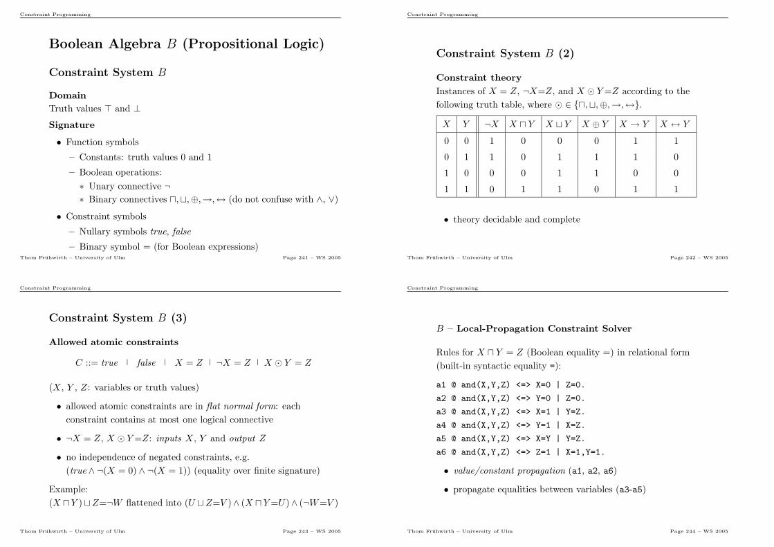
Constraint Programming
Boolean Algebra B (Propositional Logic)
Constraint System B
Domain
Truth values ⊤ and ⊥Signature
• Function symbols
– Constants: truth values 0 and 1
– Boolean operations:
∗ Unary connective ¬∗ Binary connectives ⊓,⊔,⊕,→,↔ (do not confuse with ∧, ∨)
• Constraint symbols
– Nullary symbols true, false
– Binary symbol = (for Boolean expressions)Thom Fruhwirth – University of Ulm Page 241 – WS 2005
Constraint Programming
Constraint System B (2)
Constraint theory
Instances of X = Z, ¬X=Z, and X ⊙ Y=Z according to the
following truth table, where ⊙ ∈ {⊓,⊔,⊕,→,↔}.
X Y ¬X X ⊓ Y X ⊔ Y X ⊕ Y X → Y X ↔ Y
0 0 1 0 0 0 1 1
0 1 1 0 1 1 1 0
1 0 0 0 1 1 0 0
1 1 0 1 1 0 1 1
• theory decidable and complete
Thom Fruhwirth – University of Ulm Page 242 – WS 2005
Constraint Programming
Constraint System B (3)
Allowed atomic constraints
C ::= true false X = Z ¬X = Z X ⊙ Y = Z
(X , Y , Z: variables or truth values)
• allowed atomic constraints are in flat normal form: each
constraint contains at most one logical connective
• ¬X = Z, X ⊙ Y=Z: inputs X , Y and output Z
• no independence of negated constraints, e.g.
(true ∧ ¬(X = 0) ∧ ¬(X = 1)) (equality over finite signature)
Example:
(X ⊓ Y )⊔Z=¬W flattened into (U ⊔Z=V )∧ (X ⊓ Y=U)∧ (¬W=V )
Thom Fruhwirth – University of Ulm Page 243 – WS 2005
Constraint Programming
B – Local-Propagation Constraint Solver
Rules for X ⊓ Y = Z (Boolean equality =) in relational form
(built-in syntactic equality =):
a1 @ and(X,Y,Z) <=> X=0 | Z=0.
a2 @ and(X,Y,Z) <=> Y=0 | Z=0.
a3 @ and(X,Y,Z) <=> X=1 | Y=Z.
a4 @ and(X,Y,Z) <=> Y=1 | X=Z.
a5 @ and(X,Y,Z) <=> X=Y | Y=Z.
a6 @ and(X,Y,Z) <=> Z=1 | X=1,Y=1.
• value/constant propagation (a1, a2, a6)
• propagate equalities between variables (a3-a5)
Thom Fruhwirth – University of Ulm Page 244 – WS 2005
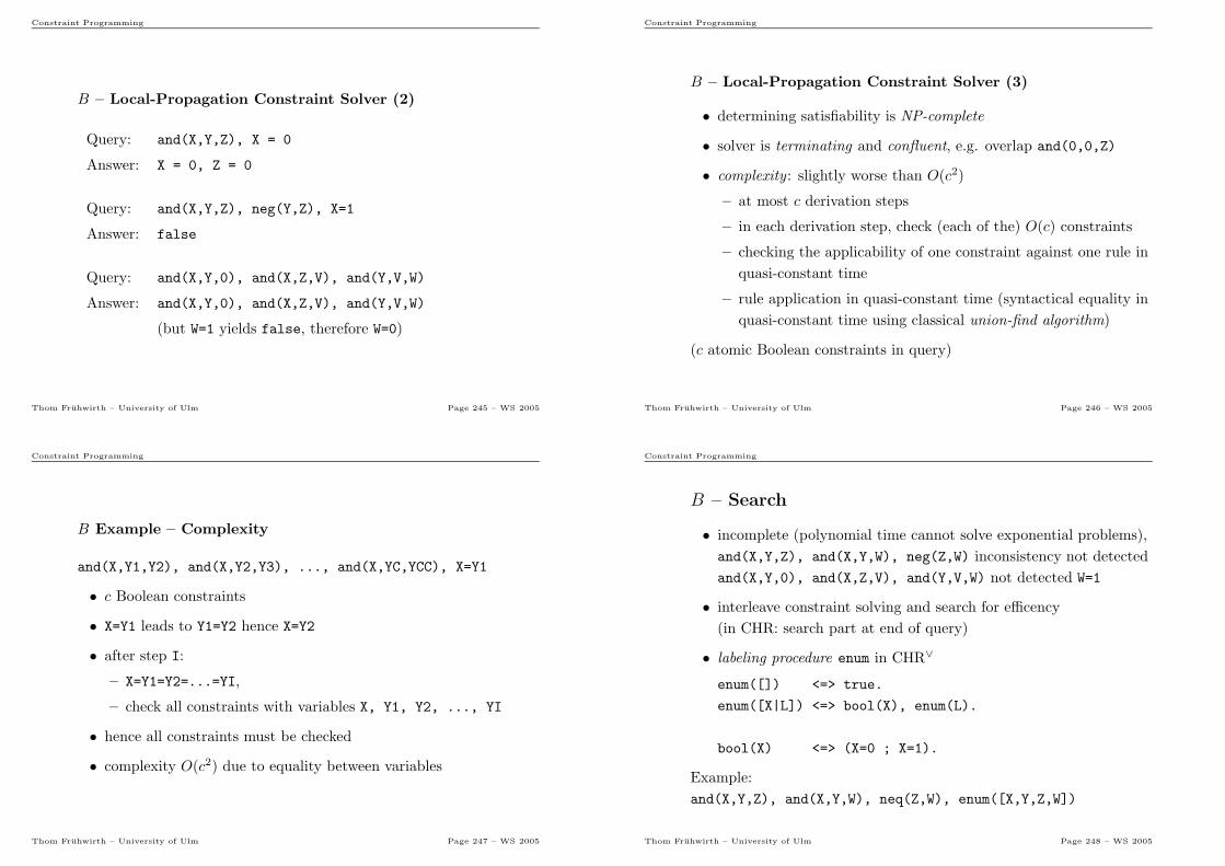
Constraint Programming
B – Local-Propagation Constraint Solver (2)
Query: and(X,Y,Z), X = 0
Answer: X = 0, Z = 0
Query: and(X,Y,Z), neg(Y,Z), X=1
Answer: false
Query: and(X,Y,0), and(X,Z,V), and(Y,V,W)
Answer: and(X,Y,0), and(X,Z,V), and(Y,V,W)
(but W=1 yields false, therefore W=0)
Thom Fruhwirth – University of Ulm Page 245 – WS 2005
Constraint Programming
B – Local-Propagation Constraint Solver (3)
• determining satisfiability is NP-complete
• solver is terminating and confluent, e.g. overlap and(0,0,Z)
• complexity : slightly worse than O(c2)
– at most c derivation steps
– in each derivation step, check (each of the) O(c) constraints
– checking the applicability of one constraint against one rule in
quasi-constant time
– rule application in quasi-constant time (syntactical equality in
quasi-constant time using classical union-find algorithm)
(c atomic Boolean constraints in query)
Thom Fruhwirth – University of Ulm Page 246 – WS 2005
Constraint Programming
B Example – Complexity
and(X,Y1,Y2), and(X,Y2,Y3), ..., and(X,YC,YCC), X=Y1
• c Boolean constraints
• X=Y1 leads to Y1=Y2 hence X=Y2
• after step I:
– X=Y1=Y2=...=YI,
– check all constraints with variables X, Y1, Y2, ..., YI
• hence all constraints must be checked
• complexity O(c2) due to equality between variables
Thom Fruhwirth – University of Ulm Page 247 – WS 2005
Constraint Programming
B – Search
• incomplete (polynomial time cannot solve exponential problems),
and(X,Y,Z), and(X,Y,W), neg(Z,W) inconsistency not detected
and(X,Y,0), and(X,Z,V), and(Y,V,W) not detected W=1
• interleave constraint solving and search for efficency
(in CHR: search part at end of query)
• labeling procedure enum in CHR∨
enum([]) <=> true.
enum([X|L]) <=> bool(X), enum(L).
bool(X) <=> (X=0 ; X=1).
Example:
and(X,Y,Z), and(X,Y,W), neq(Z,W), enum([X,Y,Z,W])
Thom Fruhwirth – University of Ulm Page 248 – WS 2005
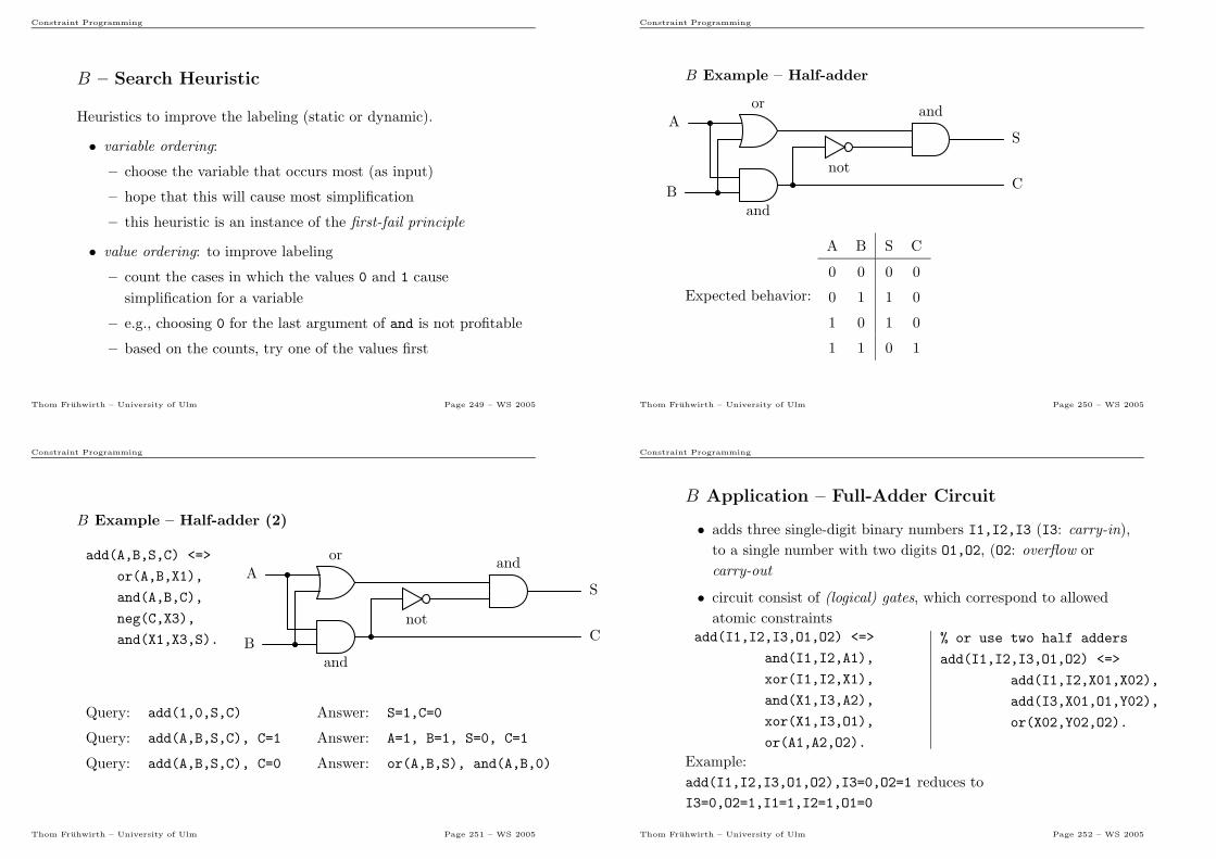
Constraint Programming
B – Search Heuristic
Heuristics to improve the labeling (static or dynamic).
• variable ordering:
– choose the variable that occurs most (as input)
– hope that this will cause most simplification
– this heuristic is an instance of the first-fail principle
• value ordering: to improve labeling
– count the cases in which the values 0 and 1 cause
simplification for a variable
– e.g., choosing 0 for the last argument of and is not profitable
– based on the counts, try one of the values first
Thom Fruhwirth – University of Ulm Page 249 – WS 2005
Constraint Programming
B Example – Half-adder
orand
and
not
A
B
S
C
Expected behavior:
A B S C
0 0 0 0
0 1 1 0
1 0 1 0
1 1 0 1
Thom Fruhwirth – University of Ulm Page 250 – WS 2005
Constraint Programming
B Example – Half-adder (2)
add(A,B,S,C) <=>
or(A,B,X1),
and(A,B,C),
neg(C,X3),
and(X1,X3,S).
orand
and
not
A
B
S
C
Query: add(1,0,S,C) Answer: S=1,C=0
Query: add(A,B,S,C), C=1 Answer: A=1, B=1, S=0, C=1
Query: add(A,B,S,C), C=0 Answer: or(A,B,S), and(A,B,0)
Thom Fruhwirth – University of Ulm Page 251 – WS 2005
Constraint Programming
B Application – Full-Adder Circuit
• adds three single-digit binary numbers I1,I2,I3 (I3: carry-in),
to a single number with two digits O1,O2, (O2: overflow or
carry-out
• circuit consist of (logical) gates, which correspond to allowed
atomic constraintsadd(I1,I2,I3,O1,O2) <=>
and(I1,I2,A1),
xor(I1,I2,X1),
and(X1,I3,A2),
xor(X1,I3,O1),
or(A1,A2,O2).
% or use two half adders
add(I1,I2,I3,O1,O2) <=>
add(I1,I2,X01,X02),
add(I3,X01,O1,Y02),
or(X02,Y02,O2).
Example:
add(I1,I2,I3,O1,O2),I3=0,O2=1 reduces to
I3=0,O2=1,I1=1,I2=1,O1=0
Thom Fruhwirth – University of Ulm Page 252 – WS 2005
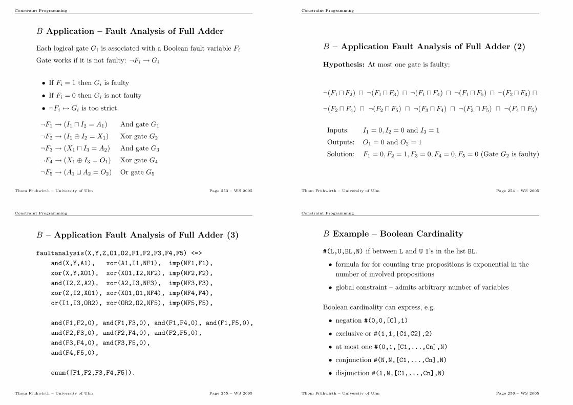
Constraint Programming
B Application – Fault Analysis of Full Adder
Each logical gate Gi is associated with a Boolean fault variable Fi
Gate works if it is not faulty: ¬Fi → Gi
• If Fi = 1 then Gi is faulty
• If Fi = 0 then Gi is not faulty
• ¬Fi ↔ Gi is too strict.
¬F1 → (I1 ⊓ I2 = A1) And gate G1
¬F2 → (I1 ⊕ I2 = X1) Xor gate G2
¬F3 → (X1 ⊓ I3 = A2) And gate G3
¬F4 → (X1 ⊕ I3 = O1) Xor gate G4
¬F5 → (A1 ⊔A2 = O2) Or gate G5
Thom Fruhwirth – University of Ulm Page 253 – WS 2005
Constraint Programming
B – Application Fault Analysis of Full Adder (2)
Hypothesis: At most one gate is faulty:
¬(F1 ⊓F2) ⊓ ¬(F1 ⊓F3) ⊓ ¬(F1 ⊓F4) ⊓ ¬(F1 ⊓F5) ⊓ ¬(F2 ⊓F3) ⊓
¬(F2 ⊓ F4) ⊓ ¬(F2 ⊓ F5) ⊓ ¬(F3 ⊓ F4) ⊓ ¬(F3 ⊓ F5) ⊓ ¬(F4 ⊓ F5)
Inputs: I1 = 0, I2 = 0 and I3 = 1
Outputs: O1 = 0 and O2 = 1
Solution: F1 = 0, F2 = 1, F3 = 0, F4 = 0, F5 = 0 (Gate G2 is faulty)
Thom Fruhwirth – University of Ulm Page 254 – WS 2005
Constraint Programming
B – Application Fault Analysis of Full Adder (3)
faultanalysis(X,Y,Z,O1,O2,F1,F2,F3,F4,F5) <=>
and(X,Y,A1), xor(A1,I1,NF1), imp(NF1,F1),
xor(X,Y,XO1), xor(XO1,I2,NF2), imp(NF2,F2),
and(I2,Z,A2), xor(A2,I3,NF3), imp(NF3,F3),
xor(Z,I2,XO1), xor(XO1,O1,NF4), imp(NF4,F4),
or(I1,I3,OR2), xor(OR2,O2,NF5), imp(NF5,F5),
and(F1,F2,0), and(F1,F3,0), and(F1,F4,0), and(F1,F5,0),
and(F2,F3,0), and(F2,F4,0), and(F2,F5,0),
and(F3,F4,0), and(F3,F5,0),
and(F4,F5,0),
enum([F1,F2,F3,F4,F5]).
Thom Fruhwirth – University of Ulm Page 255 – WS 2005
Constraint Programming
B Example – Boolean Cardinality
#(L,U,BL,N) if between L and U 1’s in the list BL.
• formula for for counting true propositions is exponential in the
number of involved propositions
• global constraint – admits arbitrary number of variables
Boolean cardinality can express, e.g.
• negation #(0,0,[C],1)
• exclusive or #(1,1,[C1,C2],2)
• at most one #(0,1,[C1,...,Cn],N)
• conjunction #(N,N,[C1,...,Cn],N)
• disjunction #(1,N,[C1,...,Cn],N)
Thom Fruhwirth – University of Ulm Page 256 – WS 2005
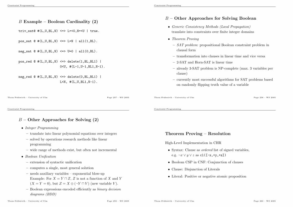
Constraint Programming
B Example – Boolean Cardinality (2)
triv_sat@ #(L,U,BL,N) <=> L=<0,N=<U | true.
pos_sat @ #(L,U,BL,N) <=> L=N | all(1,BL).
neg_sat @ #(L,U,BL,N) <=> U=0 | all(0,BL).
pos_red @ #(L,U,BL,N) <=> delete(1,BL,BL1) |
0<U, #(L-1,U-1,BL1,N-1).
neg_red @ #(L,U,BL,N) <=> delete(0,BL,BL1) |
L<N, #(L,U,BL1,N-1).
Thom Fruhwirth – University of Ulm Page 257 – WS 2005
Constraint Programming
B – Other Approaches for Solving Boolean
• Generic Consistency Methods (Local Propagation)
translate into constraints over finite integer domains
• Theorem Proving
– SAT problem: propositional Boolean constraint problem in
clausal form
– transformation into clauses in linear time and vice versa
– 2-SAT and Horn-SAT is linear time
– already 3-SAT problem is NP-complete (max. 3 variables per
clause)
– currently most successful algorithms for SAT problems based
on randomly flipping truth value of a variable
Thom Fruhwirth – University of Ulm Page 258 – WS 2005
Constraint Programming
B – Other Approaches for Solving (2)
• Integer Programming
– translate into linear polynomial equations over integers
– solved by operations research methods like linear
programming
– wide range of methods exist, but often not incremental
• Boolean Unification
– extension of syntactic unification
– computes a single, most general solution
– needs auxiliary variables – exponential blow-up
Example: For X = Y ⊓ Z, Z is not a function of X and Y
(X = Y = 0), but Z = X ⊕ (¬Y ⊓ V ) (new variable V ).
– Boolean expressions encoded efficiently as binary decision
diagrams (BDD)
Thom Fruhwirth – University of Ulm Page 259 – WS 2005
Constraint Programming
Theorem Proving – Resolution
High-Level Implementation in CHR
• Syntax: Clause as ordered list of signed variables,
e.g. ¬x ∨ y ∨ z as cl([-x,+y,+z])
• Boolean CSP in CNF: Conjunction of clauses
• Clause: Disjunction of Literals
• Literal: Positive or negative atomic proposition
Thom Fruhwirth – University of Ulm Page 260 – WS 2005
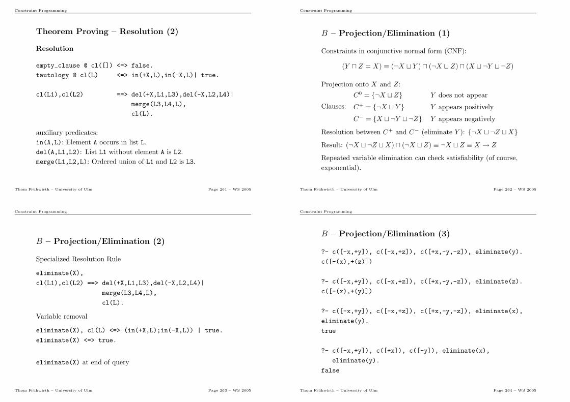
Constraint Programming
Theorem Proving – Resolution (2)
Resolution
empty_clause @ cl([]) <=> false.
tautology @ cl(L) <=> in(+X,L),in(-X,L)| true.
cl(L1),cl(L2) ==> del(+X,L1,L3),del(-X,L2,L4)|
merge(L3,L4,L),
cl(L).
auxiliary predicates:
in(A,L): Element A occurs in list L.
del(A,L1,L2): List L1 without element A is L2.
merge(L1,L2,L): Ordered union of L1 and L2 is L3.
Thom Fruhwirth – University of Ulm Page 261 – WS 2005
Constraint Programming
B – Projection/Elimination (1)
Constraints in conjunctive normal form (CNF):
(Y ⊓ Z = X) ≡ (¬X ⊔ Y ) ⊓ (¬X ⊔ Z) ⊓ (X ⊔ ¬Y ⊔ ¬Z)
Projection onto X and Z:
Clauses:
C0 = {¬X ⊔ Z} Y does not appear
C+ = {¬X ⊔ Y } Y appears positively
C− = {X ⊔ ¬Y ⊔ ¬Z} Y appears negatively
Resolution between C+ and C− (eliminate Y ): {¬X ⊔ ¬Z ⊔X}Result: (¬X ⊔ ¬Z ⊔X) ⊓ (¬X ⊔ Z) ≡ ¬X ⊔ Z ≡ X → Z
Repeated variable elimination can check satisfiability (of course,
exponential).
Thom Fruhwirth – University of Ulm Page 262 – WS 2005
Constraint Programming
B – Projection/Elimination (2)
Specialized Resolution Rule
eliminate(X),
cl(L1),cl(L2) ==> del(+X,L1,L3),del(-X,L2,L4)|
merge(L3,L4,L),
cl(L).
Variable removal
eliminate(X), cl(L) <=> (in(+X,L);in(-X,L)) | true.
eliminate(X) <=> true.
eliminate(X) at end of query
Thom Fruhwirth – University of Ulm Page 263 – WS 2005
Constraint Programming
B – Projection/Elimination (3)
?- c([-x,+y]), c([-x,+z]), c([+x,-y,-z]), eliminate(y).
c([-(x),+(z)])
?- c([-x,+y]), c([-x,+z]), c([+x,-y,-z]), eliminate(z).
c([-(x),+(y)])
?- c([-x,+y]), c([-x,+z]), c([+x,-y,-z]), eliminate(x),
eliminate(y).
true
?- c([-x,+y]), c([+x]), c([-y]), eliminate(x),
eliminate(y).
false
Thom Fruhwirth – University of Ulm Page 264 – WS 2005
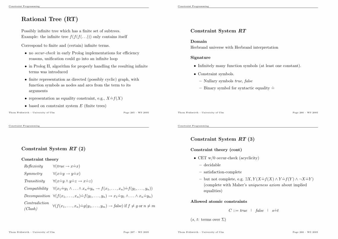
Constraint Programming
Rational Tree (RT)
Possibly infinite tree which has a finite set of subtrees.
Example: the infinite tree f(f(f(. . .))) only contains itself
Correspond to finite and (certain) infinite terms.
• no occur-check in early Prolog implementations for efficiency
reasons, unification could go into an infinite loop
• in Prolog II, algorithm for properly handling the resulting infinite
terms was introduced
• finite representation as directed (possibly cyclic) graph, with
function symbols as nodes and arcs from the term to its
arguments
• representation as equality constraint, e.g., X=f(X)
• based on constraint system E (finite trees)
Thom Fruhwirth – University of Ulm Page 265 – WS 2005
Constraint Programming
Constraint System RT
Domain
Herbrand universe with Herbrand interpretation
Signature
• Infinitely many function symbols (at least one constant).
• Constraint symbols.
– Nullary symbols true, false
– Binary symbol for syntactic equality =
Thom Fruhwirth – University of Ulm Page 266 – WS 2005
Constraint Programming
Constraint System RT (2)
Constraint theory
Reflexivity ∀(true→ x=x)
Symmetry ∀(x=y → y=x)
Transitivity ∀(x=y ∧ y=z → x=z)
Compatibility ∀(x1=y1 ∧ . . . ∧ xn=yn → f(x1, . . . , xn)=f(y1, . . . , yn))
Decomposition ∀(f(x1, . . . , xn)=f(y1, . . . , yn)→ x1=y1 ∧ . . . ∧ xn=yn)
Contradiction
(Clash)∀(f(x1, . . . , xn)=g(y1, . . . , ym)→ false) if f 6= g or n 6= m
Thom Fruhwirth – University of Ulm Page 267 – WS 2005
Constraint Programming
Constraint System RT (3)
Constraint theory (cont)
• CET w/0 occur-check (acyclicity)
– decidable
– satisfaction-complete
– but not complete, e.g. ∃X,Y (X=f(X) ∧ Y =f(Y ) ∧ ¬X=Y )
(complete with Maher’s uniqueness axiom about implied
equalities)
Allowed atomic constraints
C ::= true false s=t
(s, t: terms over Σ)
Thom Fruhwirth – University of Ulm Page 268 – WS 2005

Constraint Programming
RT – Solved Normal Form
Conjunction of allowed constraints is solved (in solved normal form):
• false or
• X1=t1 ∧ . . . ∧Xn=tn (n ≥ 0)
– X1, . . . , Xn pairwise distinct
– Xi different to tj if i ≤ j
Thom Fruhwirth – University of Ulm Page 269 – WS 2005
Constraint Programming
RT – Solved Normal Form (2)
Examples:
• not in solved normal form:
f(X, b)=f(a, Y ), or X=t ∧X=s, or X=Y ∧ Y =X
• in solved normal form:
logically equivalent but syntactically different forms:
X=Y and Y =X
X=f(X) and X=f(f(X))
X=Z ∧ Y =Z ∧ Z=t and X=t ∧ Y =t ∧ Z=t
From solved normal form we can read off the most general unifier:
Each equation Xi=ti as substitution Xi 7→ ti.
Thom Fruhwirth – University of Ulm Page 270 – WS 2005
Constraint Programming
RT – Variable Elimination Constraint Solver
reflexivity @ X eq X <=> var(X) | true.
orientation @ T eq X <=> var(X),X@<T | X eq T.
decomposition @ T1 eq T2 <=> nonvar(T1),nonvar(T2) |
same_functor(T1,T2),
args2list(T1,L1),args2list(T2,L2),
same_args(L1,L2).
confrontation @ X eq T1, X eq T2 <=> var(X),X@<T1,T1@=<T2 |
X eq T1, T1 eq T2.
• confrontation rule: restricted form of variable elimination
• satisfaction complete: produces solved normal form (while not in
solved normal form one of the rules is applicable)
Thom Fruhwirth – University of Ulm Page 271 – WS 2005
Constraint Programming
RT – Variable Elimination Constraint Solver (2)
Auxiliary constraints
• For termination:
s@<t : given total strict order on terms that holds at least
– if size of s is less than size of t
(size: number of occurrences of function symbols)
• For term manipulation:
– var(X), nonvar(X): variable, function term
– same_functor(T1,T2): T1 and T2 have the same function
symbol and the same arity
– args2list(T1,L1): L1 is the guarded list of arguments of the
term T1
Thom Fruhwirth – University of Ulm Page 272 – WS 2005
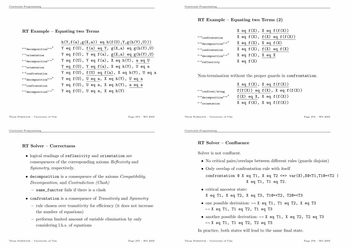
Constraint Programming
RT Example – Equating two Terms
h(Y,f(a),g(X,a)) eq h(f(U),Y,g(h(Y),U)))
7→decomposition 7→∗ Y eq f(U), f(a) eq Y, g(X,a) eq g(h(Y),U)
7→orientation Y eq f(U), Y eq f(a), g(X,a) eq g(h(Y),U)
7→decomposition 7→∗ Y eq f(U), Y eq f(a), X eq h(Y), a eq U
7→orientation Y eq f(U), Y eq f(a), X eq h(Y), U eq a
7→confrontation Y eq f(U), f(U) eq f(a), X eq h(Y), U eq a
7→decomposition 7→∗ Y eq f(U), U eq a, X eq h(Y), U eq a
7→confrontation Y eq f(U), U eq a, X eq h(Y), a eq a
7→decomposition 7→∗ Y eq f(U), U eq a, X eq h(Y)
Thom Fruhwirth – University of Ulm Page 273 – WS 2005
Constraint Programming
RT Example – Equating two Terms (2)
X eq f(X), X eq f(f(X))
7→confrontation X eq f(X), f(X) eq f(f(X))
7→decomposition 7→∗ X eq f(X), X eq f(X)
7→confrontation X eq f(X), f(X) eq f(X)
7→decomposition 7→∗ X eq f(X), X eq X
7→reflexivity X eq f(X)
Non-termination without the proper guards in confrontation:
X eq f(X), X eq f(f(X))
7→confront/wrong f(f(X)) eq f(X), X eq f(f(X))
7→decomposition 7→∗ f(X) eq X, X eq f(f(X))
7→orientation X eq f(X), X eq f(f(X))
Thom Fruhwirth – University of Ulm Page 274 – WS 2005
Constraint Programming
RT Solver – Correctness
• logical readings of reflexivity and orientation are
consequences of the corresponding axioms Reflexivity and
Symmetry, respectively.
• decomposition is a consequence of the axioms Compatibility,
Decomposition, and Contradiction (Clash)
– same_functor fails if there is a clash
• confrontation is a consequence of Transitivity and Symmetry
– rule chosen over transitivity for efficiency (it does not increase
the number of equations)
– performs limited amount of variable elimination by only
considering l.h.s. of equations
Thom Fruhwirth – University of Ulm Page 275 – WS 2005
Constraint Programming
RT Solver – Confluence
Solver is not confluent.
• No critical pairs/overlaps between different rules (guards disjoint)
• Only overlap of confrontation rule with itself
confrontation @ X eq T1, X eq T2 <=> var(X),X@<T1,T1@=<T2 |
X eq T1, T1 eq T2.
• critical ancestor state:
X eq T1, X eq T2, X eq T3, T1@=<T2, T2@=<T3
• one possible derivation: 7→ X eq T1, T1 eq T2, X eq T3
7→ X eq T1, T1 eq T2, T1 eq T3
• another possible derivation: 7→ X eq T1, X eq T2, T2 eq T3
7→ X eq T1, T1 eq T2, T2 eq T3
In practice, both states will lead to the same final state.
Thom Fruhwirth – University of Ulm Page 276 – WS 2005
Constraint Programming
RT Application – Program Analysis
In general, rational trees can represent directed graphs, e.g.,
automata.
Here we use rational trees to represent a recursive data type and to
type check terms with it.
A list is defined recursively as
• constant nil
• binary list constructor cons applied to a term of type Element
and to a list
Type of lists
List eq (nil or cons(Element,List)).
(or: binary infix operator separating alternatives)
Thom Fruhwirth – University of Ulm Page 277 – WS 2005
Constraint Programming
RT Application – Program Analysis (2)
Type checker: Term of Type if Term is of type Type
Term of (Type1 or Type2) <=> (Term of Type1 ; Term of Type2).
Term of Type <=> nonvar(Term),nonvar(Type) |
same_functor(Term,Type),
args2list(Term,Args),args2list(Type,Types),
check_args(Args,Types).
Term of Type, Type eq Type1 <=> var(Type) |
Term of Type1, Type eq Type1.
check_args([],[]) <=> true.
check_args([Arg|Args],[Type|Types]) <=>
Arg of Type, check_args(Args,Types).
Thom Fruhwirth – University of Ulm Page 278 – WS 2005
Constraint Programming
RT Application – Program Analysis (3)
• generate the type or lists with
list(List, Element) <=> List eq (nil or cons(Element,List)).
• list(NL,(0 or 1 or ...or 9)) lists over single-digit numbers
• cons(3,cons(0,nil)) of NL performs a type check:
cons(3,cons(0,nil)) eq (nil or cons((0 or 1 or ... or
9), NL))
– either:
cons(3,cons(0,nil)) of nil (fails)
– or:
cons(3,cons(0,nil)) of cons(0 or 1 or ... or 9,NL)
check_args([3,cons(0,nil)],[0 or 1 or ... or 9,NL])
3 of 0 or 1 or ... or 9, cons(0,nil) of NL
Thom Fruhwirth – University of Ulm Page 279 – WS 2005
Constraint Programming
Feature Terms (FTs)
Feature terms allow to model records in logic (originally from
linguistics).
Motivation
Prolog Herbrand terms.
Pros: universal, flexible data structure
Cons: position-based access, hard to extend
• features: selectors (attributes/name-based access)
• sort : type name of record
• can be represented as graphs:
sorts are nodes, features are arcs
• feature trees can represent rational trees and vice versa
Thom Fruhwirth – University of Ulm Page 280 – WS 2005
Constraint Programming
Constraint System FT
Signature
• Infinitely many constants
• Constraint symbols:
– unary sorts s
– binary features f
– =, true, and false
Domain
Infinite set of individuals (constants).
Thom Fruhwirth – University of Ulm Page 281 – WS 2005
Constraint Programming
Constraint System FT (2)
Constraint theory
Equivalence relation = over variables and constants
(refl., symm., trans.)
X f Y ∧X f Z ⇒ Y = Z
a(X) ∧ b(X)⇒ false if a 6= b
Allowed atomic constraints
C ::= true false s(X) X f Y X = Y
(s: sort, f : feature in infix notation)
Thom Fruhwirth – University of Ulm Page 282 – WS 2005
Constraint Programming
FT – Solved Normal Form
Conjunction of allowed constraints is solved (in solved normal form):
• false (due to different sorts)
• if each variable comes in at most one sort constraint and at most
once in the left hand side of an equation or particular feature
constraint
Thom Fruhwirth – University of Ulm Page 283 – WS 2005
Constraint Programming
FT – Solved Normal Form (2)
Example:
person(X) ∧X name Y ∧ Y = leo ∧X livesIn Z ∧munich(Z)∧X name V ∧ V = sepp
• by CT V = Y , replace V by Y
• by CT Y = leo and sepp(Y ) leads to false
Note: person(X) ∧X name Y ∧ Y = leo ∧X livesIn Z ∧munich(Z)
can be compactly written as X:person(name=leo,livesIn=munich)
Thom Fruhwirth – University of Ulm Page 284 – WS 2005
Constraint Programming
FT – Constraint Solver
equal @ X eq Y <=> X=Y.
feature @ X.F.Y \ X.F.Z <=> Y=Z.
sort @ X:S1 \ X:S2 <=> S1=S2.
• – =: eq, =
– s(X): X:s
– X f Y : X.f.Y
• constraint solver uses built-in unification (=) between variables
and constants
• equal: variable elimination
• feature: feature decomposition (functional)
• sort: sort intersection
Thom Fruhwirth – University of Ulm Page 285 – WS 2005
Constraint Programming
FT – Constraint Solver (2)
FT – Properties of Solver
• Correctness: rules obvious logical consequences of corresponding
axioms.
• Termination: obvious, since each rule removes one CHR
constraint.
• No Confluence: no overlays between different rules, but sort and
feature rule can overlap with themselves, e.g., X.F.Y, X.F.Z
yields X.F.Y, Y=Z or X.F.Z, Z=Y.
• Complexity: number of rule trials and applications linear in
number of constraints if indexing is used for sorts and
variable-feature pairs. Rule applications take constant time if
built-in equality takes constant time (possible with union-find
algorithm).
Thom Fruhwirth – University of Ulm Page 286 – WS 2005
Constraint Programming
FT – Constraint Solver (3)
Extension: Negation
Added to allowed constraints:
¬s(X)
¬X f (shorthand for ∀Y ¬(X f Y ))
Added to formulas of CT:
s(X) ∧ ¬s(X)⇒ false
X f Y ∧ ¬X f ⇒ false
Added to rules of constraint solver:
X:S, not X:S <=> false.
X.F.Z, not X.F <=> false.
Thom Fruhwirth – University of Ulm Page 287 – WS 2005
Constraint Programming
FT – Constraint Solver (4)
Extension: Arity Constraints
Herbrand-Term X = g(Y, Z) can be written as g(X)∧X 1 Y ∧X 2 Z.
Forbid additional features like X 3 V by explicitly stating allowed
features (here X{1, 2}) (also useful to explicitly disallow definition of
new features, e.g. X{livesIn, name}.)
Added to allowed constraints:
X{f1, . . . , fn}
(Variant: S{f1, . . . , fn}, S sort not sufficient with free Herbrand
terms)
Thom Fruhwirth – University of Ulm Page 288 – WS 2005
Constraint Programming
FT – Constraint Solver (5)
Extension: Arity Constraints (cont)
Added to formulas of CT:
X F ∧X G⇒ false if F 6= G
X F ∧X f Y ⇒ false if f 6∈ F
Added to rules of constraint solver (Fs, G ordered lists of features):
X in Fs \ X in G <=> Fs=G.
X in Fs, X.F.Y ==> member(F,Fs).
Another possible extension:
Ordered sorted feature trees allow hierarchies (Ait-Kaci et al. 93).
Thom Fruhwirth – University of Ulm Page 289 – WS 2005
Constraint Programming
FT Example – Linguistics
FT use in knowledge representation in linguistics, e.g. to describe the
contents of a sentence.
X = ∃Y
Person
office : Y
home : Y
name :
first : Leo
last : Smith
Person(X) ∧X office Y ∧X home Y ∧X name N ∧N first S1∧S1 = Leo ∧N last S2 ∧ S2 = Smith
Thom Fruhwirth – University of Ulm Page 290 – WS 2005
Constraint Programming
Description Logics (DL)
Terminological Reasoning
Rich formalism for knowledge representation (originating in
Brachman’s KL-ONE, 1980s).
Concepts (unary constraints): properties like human, car (not
disjunct).
Roles (binary constraints): relations like child, age (not functional
dependent).
Graph representation: concepts are nodes, roles are arcs.
By default, concepts do not exclude each other.
Rich subset of first order logic to define concepts:
parent isa human and some child is human
Multiple inheritance possible. Related to type systems.Thom Fruhwirth – University of Ulm Page 291 – WS 2005
Constraint Programming
DL – Knowledge Representation
Two kinds of knowledge:
Terminological knowledge (T-Box)
General background knowledge of the application domain.
Intensional representation (like database scheme).
Concepts are defined by other concepts and restrictions on roles.
T-Box does not contain variables and individuals.
parent isa human and some child is human
Assertional knowledge (A-Box)
Concrete problem-specific knowledge.
Extensional representation (like database extension) that is checked
against T-Box.
Statements about concepts and roles of individuals (objects).
sue:parent, (sue,joe):child
Thom Fruhwirth – University of Ulm Page 292 – WS 2005
Constraint Programming
Constraint System DL
Domain
Infinite set of individuals (constants).
Signature
Infinitely many constants for individuals, concept and role names.
Function symbols and, or, not, every, some, is for building concept
terms involving concept and role names.
Constraint symbols: true, false, isa (definitions) and “:” (assertions).
Allowed Constraints
C ::= true false I : s (I, J) : r
A-Box: I : s membership, (I, J) : r role filler
T-Box: c isa s concept definition with concept name c implemented
as a rule
(I, J : variables or individuals, r role name, s concept term)Thom Fruhwirth – University of Ulm Page 293 – WS 2005
Constraint Programming
Constraint System DL (2)
Concept Term s
A concept (name) c, or one of:
not s, s and t, s or t, some r is s, every r is s,
where s and t are concept terms.
Constraint Theory
I : not S ↔ ¬(I : S)
I : S1 and S2 ↔ I : S1 ∧ I : S2
I : S1 or S2 ↔ I : S1 ∨ I : S2
I : some R is S ↔ ∃J((I, J) : R ∧ J : S)
I : every R is S ↔ ((I, J) : R→ J : S) (also holds if no (I, J) : R)
C isa S ↔ (I : C ↔ I : S)
Thom Fruhwirth – University of Ulm Page 294 – WS 2005
Constraint Programming
DL – Solved Normal Form
Conjunction of allowed constraints of form
• false
• I : Ci, I : not Cj where Ci, Cj are primitive (undefined) concepts
(Ci 6= Cj)
I : every R is S, (I, J) : R (unchanged)
Thom Fruhwirth – University of Ulm Page 295 – WS 2005
Constraint Programming
DL – Constraint Solver (1)
Direct implementation of theory: A-Box as constraints, T-Box as
rules. (Variant: T-Box as constraints)
Produces solved normal form that shows inconsistency. (Only
membership constraints change.)
Split membership constraints:
I:S1 and S2 <=> I:S1, I:S2.
I:some R is S <=> (I,J):R, J:S.
I:every R is S, (I,J):R ==> J:S.
label, I:S1 or S2 <=> true | (I:S1 ; I:S2), label. % search
Thom Fruhwirth – University of Ulm Page 296 – WS 2005
Constraint Programming
DL – Constraint Solver (2)
Negation
I:not not S <=> I:S.
I:not (S1 and S2) <=> I:not S1 or not S2.
I:not (S1 or S2) <=> I:not S1 and not S2.
I:not (some R is S) <=> I:every R is not S.
I:not (every R is S) <=> I:some R is not S.
Clash Rule
I:not S, I:S <=> false.
For each concept definition C isa S (unfold definitions)
I:C <=> I:S.
I:not C <=> I:not S.
(T-Box as constraint: C isa S \ I:C <=> I:S).
Thom Fruhwirth – University of Ulm Page 297 – WS 2005
Constraint Programming
DL – Family Relationships Example T-Box
male isa not female.
parent isa human and some child is human.
mother isa parent and female.
proud_parent isa parent and every child is phd.
Undefined concepts are called primitive:
female, human and phd.
Implicit concept hierarchy (taxonomy) with multiple inheritance:
parent<human, mother<parent, mother<female,
proud_parent<parent.
Notes:
Cyclic definitions (female isa not male)
Completion by human isa female or male
Thom Fruhwirth – University of Ulm Page 298 – WS 2005
Constraint Programming
DL – Family Relationships Example A-Box
sue:proud_parent, (sue,joe):child, joe:not phd.
- Unfold concept definition proud_parent
sue:parent and every child is phd,...
- Unfold concept definition parent and split and
sue:human, sue:some child is human, sue:every child is
phd,...
- Simplify exists-in restriction some
sue:human, (sue,X):child, X:human, sue:every child is
phd,...
- Propagate value restriction every
X:phd, joe:phd, sue:human, (sue,X):child, X:human,
sue:every child is phd, (sue,joe):child, joe:not phd.
- Clash between joe:phd and joe:not phd
Note: X may be joe, but need not to be.
Thom Fruhwirth – University of Ulm Page 299 – WS 2005
Constraint Programming
DL – Some Extensions
all quantifiers:
parent isa human and all child is human
I:all R is S <=> I:every R is S,I:some R is S
Role chains (nested roles):
grandfather isa father of father
(I,J):A of B <=> (I,K):A, (K,J):B
Functional roles (features, attributes) (subsumes FT):
(I,J):F, (I,K):F ==> functional(F) | J=K.
Distinct, disjoint primitive concepts (useful for FT):
I:C1, I:C2 ==> distinct(C1) | C1=C2.
Concrete domains:
(I,J):smaller ==> I<J.
(Conjecture: FT-like arity constraint needed to represent rational trees.)
Thom Fruhwirth – University of Ulm Page 300 – WS 2005
Constraint Programming
DL – Applications
Assessing the contents of web pages (XML, OWL).
Represent medical knowledge (illnesses).
Configuration of technical systems (e.g. PC peripherals).
Thom Fruhwirth – University of Ulm Page 301 – WS 2005
Constraint Programming
Linear Polynomial Equations ℜ
Constraint System ℜ
Domain
The set ℜ of real numbers.
Signature
• Function symbols.
– The real numbers 0 and 1
– Unary prefix operators + and −– Binary infix operators + and ∗
• Constraint symbols.
– Nullary symbols true, false
– Binary symbols =, <,≤, >,≥, 6=Thom Fruhwirth – University of Ulm Page 302 – WS 2005
Constraint Programming
Constraint System ℜ (2)
Constraint theory
The linear existential fragment of Tarski’s axiomatic theory of real
closed fields for elementary geometry.
Allowed atomic constraints
Linear equations and inequations:
C ::= true false a1 ∗X1 + . . .+ an ∗Xn + b ⊙ 0, (n ≥ 0)
• coefficients ai, b ∈ ℜ, ai 6= 0,
• variables X1, . . . , Xn totally ordered in strictly descending order
• ⊙ ∈ {=, <,≤, >,≥, 6=}
The l.h.s. of the equation is called (linear) polynomial.
Thom Fruhwirth – University of Ulm Page 303 – WS 2005
Constraint Programming
ℜ – Real closed fields
Decidable constraint theory for real arithmetic from Tarski.
C1 (x+ y) + z = x+ (y + z) associative (+)
C2 x+ 0 = x neutral element (+)
C3 x+ (−1 ∗ x) = 0 inverse element (+)
C4 x+ y = y + x commutative (+)
C5 (x ∗ y) ∗ z = x ∗ (y ∗ z) associative (∗)C6 x ∗ 1 = x neutral element (∗)C7 x 6= 0→ ∃y x ∗ y = 1 inverse element (∗)C8 x ∗ y = y ∗ x commutative (∗)C9 x ∗ (y + z) = (x ∗ y) + (x ∗ z) distributive
C10 0 6= 1
Thom Fruhwirth – University of Ulm Page 304 – WS 2005
Constraint Programming
ℜ – Real closed fields (2)
O1 ¬(x < x) irreflexive
O2 x < y ∧ y < z → x < z transitive
O3 x < y ∨ x = y ∨ y < x total order
O4 x < y → x+ z → y + z
O5 0 < x ∧ 0 < y → 0 < x ∗ yR1 0 < x→ ∃y y ∗ y = x
R2yn 6= 0→ ∃x yn ∗ xn + yn−1 ∗ xn−1 + · · ·+ y0 = 0
for every odd n
Thom Fruhwirth – University of Ulm Page 305 – WS 2005
Constraint Programming
ℜ – Tarski’s theory
• theory is complete and decidable, but intractable
• covers linear and non-linear polynomials
• linear existential fragment is decidable in polynomial time
• but only refers to the real numbers 0 and 1
Thom Fruhwirth – University of Ulm Page 306 – WS 2005
Constraint Programming
ℜ – Variable Elimination Constraint Solver
• incremental variants of classical variable elimination algorithms
– Gaussian elimination for equations (cubic complexity in
number of different variables)
– Dantzig’s Simplex algorithm for equations and inequations
(exponential worst case complexity but polynomial on
average)
• implementation problems
– reals: approximated by floating-point numbers, with
unavoidable rounding errors (partial remedy: avoid using
variables for elimination that have a small coefficient)
– rationals: precise, size can grow exponentially in the size of
the problem due to multiplication operations
Thom Fruhwirth – University of Ulm Page 307 – WS 2005
Constraint Programming
ℜ – Variable Elimination Constraint Solver (2)
Conjunction of allowed constraints is solved (in solved normal form):
• false or
• left-most variable of each equation does not appear in any other
equation
Compute solved form by eliminating multiple occurrences of
variables, eliminate variables one by one:
• choose an equation a1 ∗X1 + . . .+ an ∗Xn + b = 0
• make its left-most variable explicit:
X1 = −(a2 ∗X2 + . . .+ an ∗Xn + b)/a1
• replace all other occurrences of X1 by
−(a2 ∗X2 + . . .+ an ∗Xn + b)/a1
• simplify resulting equations into allowed constraints
Thom Fruhwirth – University of Ulm Page 308 – WS 2005
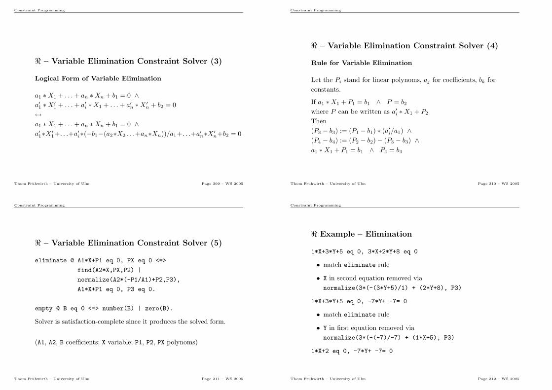
Constraint Programming
ℜ – Variable Elimination Constraint Solver (3)
Logical Form of Variable Elimination
a1 ∗X1 + . . .+ an ∗Xn + b1 = 0 ∧a′1 ∗X ′
1 + . . .+ a′i ∗X1 + . . .+ a′n ∗X ′n + b2 = 0
↔a1 ∗X1 + . . .+ an ∗Xn + b1 = 0 ∧a′1∗X ′
1+. . .+a′i∗(−b1−(a2∗X2 . . .+an∗Xn))/a1+. . .+a′n∗X ′n+b2 = 0
Thom Fruhwirth – University of Ulm Page 309 – WS 2005
Constraint Programming
ℜ – Variable Elimination Constraint Solver (4)
Rule for Variable Elimination
Let the Pi stand for linear polynoms, aj for coefficients, bk for
constants.
If a1 ∗X1 + P1 = b1 ∧ P = b2
where P can be written as a′i ∗X1 + P2
Then
(P3 − b3) := (P1 − b1) ∗ (a′i/a1) ∧(P4 − b4) := (P2 − b2)− (P3 − b3) ∧a1 ∗X1 + P1 = b1 ∧ P4 = b4
Thom Fruhwirth – University of Ulm Page 310 – WS 2005
Constraint Programming
ℜ – Variable Elimination Constraint Solver (5)
eliminate @ A1*X+P1 eq 0, PX eq 0 <=>
find(A2*X,PX,P2) |
normalize(A2*(-P1/A1)+P2,P3),
A1*X+P1 eq 0, P3 eq 0.
empty @ B eq 0 <=> number(B) | zero(B).
Solver is satisfaction-complete since it produces the solved form.
(A1, A2, B coefficients; X variable; P1, P2, PX polynoms)
Thom Fruhwirth – University of Ulm Page 311 – WS 2005
Constraint Programming
ℜ Example – Elimination
1*X+3*Y+5 eq 0, 3*X+2*Y+8 eq 0
• match eliminate rule
• X in second equation removed via
normalize(3*(-(3*Y+5)/1) + (2*Y+8), P3)
1*X+3*Y+5 eq 0, -7*Y+ -7= 0
• match eliminate rule
• Y in first equation removed via
normalize(3*(-(-7)/-7) + (1*X+5), P3)
1*X+2 eq 0, -7*Y+ -7= 0
Thom Fruhwirth – University of Ulm Page 312 – WS 2005
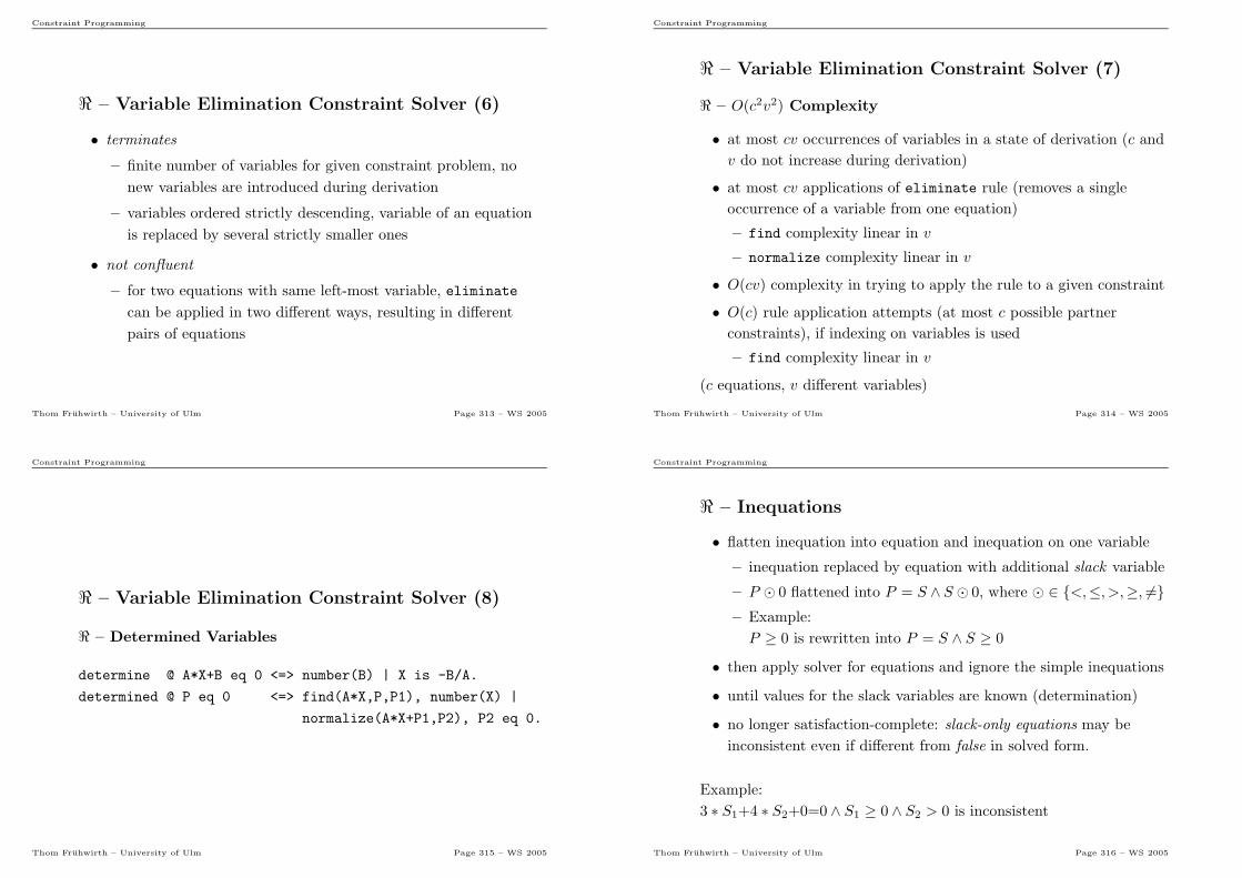
Constraint Programming
ℜ – Variable Elimination Constraint Solver (6)
• terminates
– finite number of variables for given constraint problem, no
new variables are introduced during derivation
– variables ordered strictly descending, variable of an equation
is replaced by several strictly smaller ones
• not confluent
– for two equations with same left-most variable, eliminate
can be applied in two different ways, resulting in different
pairs of equations
Thom Fruhwirth – University of Ulm Page 313 – WS 2005
Constraint Programming
ℜ – Variable Elimination Constraint Solver (7)
ℜ – O(c2v2) Complexity
• at most cv occurrences of variables in a state of derivation (c and
v do not increase during derivation)
• at most cv applications of eliminate rule (removes a single
occurrence of a variable from one equation)
– find complexity linear in v
– normalize complexity linear in v
• O(cv) complexity in trying to apply the rule to a given constraint
• O(c) rule application attempts (at most c possible partner
constraints), if indexing on variables is used
– find complexity linear in v
(c equations, v different variables)
Thom Fruhwirth – University of Ulm Page 314 – WS 2005
Constraint Programming
ℜ – Variable Elimination Constraint Solver (8)
ℜ – Determined Variables
determine @ A*X+B eq 0 <=> number(B) | X is -B/A.
determined @ P eq 0 <=> find(A*X,P,P1), number(X) |
normalize(A*X+P1,P2), P2 eq 0.
Thom Fruhwirth – University of Ulm Page 315 – WS 2005
Constraint Programming
ℜ – Inequations
• flatten inequation into equation and inequation on one variable
– inequation replaced by equation with additional slack variable
– P ⊙ 0 flattened into P = S ∧ S ⊙ 0, where ⊙ ∈ {<,≤, >,≥, 6=}– Example:
P ≥ 0 is rewritten into P = S ∧ S ≥ 0
• then apply solver for equations and ignore the simple inequations
• until values for the slack variables are known (determination)
• no longer satisfaction-complete: slack-only equations may be
inconsistent even if different from false in solved form.
Example:
3 ∗ S1+4 ∗ S2+0=0 ∧ S1 ≥ 0 ∧ S2 > 0 is inconsistent
Thom Fruhwirth – University of Ulm Page 316 – WS 2005
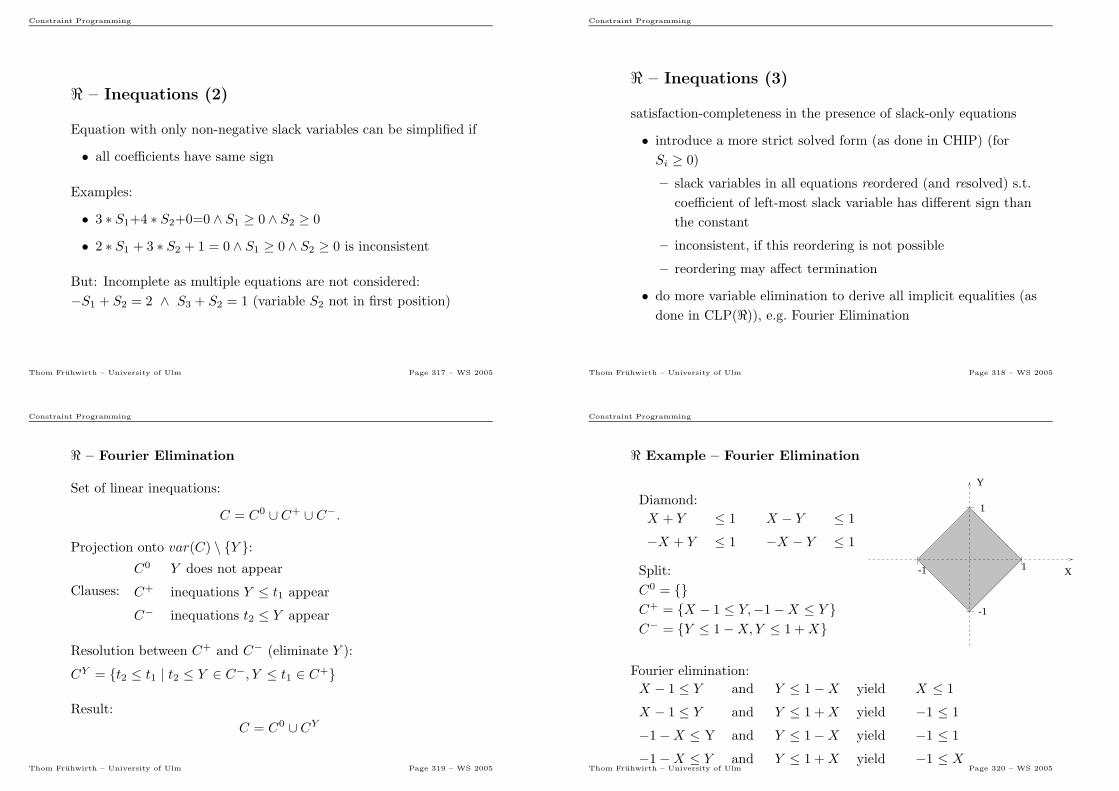
Constraint Programming
ℜ – Inequations (2)
Equation with only non-negative slack variables can be simplified if
• all coefficients have same sign
Examples:
• 3 ∗ S1+4 ∗ S2+0=0 ∧ S1 ≥ 0 ∧ S2 ≥ 0
• 2 ∗ S1 + 3 ∗ S2 + 1 = 0 ∧ S1 ≥ 0 ∧ S2 ≥ 0 is inconsistent
But: Incomplete as multiple equations are not considered:
−S1 + S2 = 2 ∧ S3 + S2 = 1 (variable S2 not in first position)
Thom Fruhwirth – University of Ulm Page 317 – WS 2005
Constraint Programming
ℜ – Inequations (3)
satisfaction-completeness in the presence of slack-only equations
• introduce a more strict solved form (as done in CHIP) (for
Si ≥ 0)
– slack variables in all equations reordered (and resolved) s.t.
coefficient of left-most slack variable has different sign than
the constant
– inconsistent, if this reordering is not possible
– reordering may affect termination
• do more variable elimination to derive all implicit equalities (as
done in CLP(ℜ)), e.g. Fourier Elimination
Thom Fruhwirth – University of Ulm Page 318 – WS 2005
Constraint Programming
ℜ – Fourier Elimination
Set of linear inequations:
C = C0 ∪ C+ ∪ C−.
Projection onto var(C) \ {Y }:
Clauses:
C0 Y does not appear
C+ inequations Y ≤ t1 appear
C− inequations t2 ≤ Y appear
Resolution between C+ and C− (eliminate Y ):
CY = {t2 ≤ t1 | t2 ≤ Y ∈ C−, Y ≤ t1 ∈ C+}
Result:
C = C0 ∪ CY
Thom Fruhwirth – University of Ulm Page 319 – WS 2005
Constraint Programming
ℜ Example – Fourier Elimination
Diamond:
X + Y ≤ 1 X − Y ≤ 1
−X + Y ≤ 1 −X − Y ≤ 1
Split:
C0 = {}C+ = {X − 1 ≤ Y,−1−X ≤ Y }C− = {Y ≤ 1−X,Y ≤ 1 +X}
X
Y
1-1
1
-1
Fourier elimination:
X − 1 ≤ Y and Y ≤ 1−X yield X ≤ 1
X − 1 ≤ Y and Y ≤ 1 +X yield −1 ≤ 1
−1−X ≤ Y and Y ≤ 1−X yield −1 ≤ 1
−1−X ≤ Y and Y ≤ 1 +X yield −1 ≤ XThom Fruhwirth – University of Ulm Page 320 – WS 2005
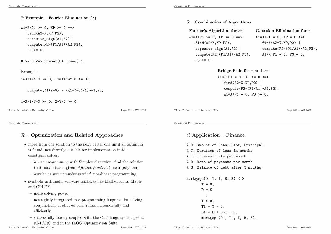
Constraint Programming
ℜ Example – Fourier Elimination (2)
A1*X+P1 >= 0, XP >= 0 ==>
find(A2*X,XP,P2),
opposite_sign(A1,A2) |
compute(P2-(P1/A1)*A2,P3),
P3 >= 0.
B >= 0 <=> number(B) | geq(B).
Example:
1*X+1*Y+0 >= 0, -1*X+1*Y+0 >= 0,
compute((1*Y+0) - ((1*Y+0)/1)*-1,P3)
1*X+1*Y+0 >= 0, 2*Y+0 >= 0
Thom Fruhwirth – University of Ulm Page 321 – WS 2005
Constraint Programming
ℜ – Combination of Algorithms
Fourier’s Algorithm for >=
A1*X+P1 >= 0, XP >= 0 ==>
find(A2*X,XP,P2),
opposite_sign(A1,A2) |
compute(P2-(P1/A1)*A2,P3),
P3 >= 0.
Gaussian Elimination for =
A1*X+P1 = 0, XP = 0 <=>
find(A2*X,XP,P2) |
compute(P2-(P1/A1)*A2,P3),
A1*X+P1 = 0, P3 = 0.
Bridge Rule for = and >=
A1*X+P1 = 0, XP >= 0 <=>
find(A2*X,XP,P2) |
compute(P2-(P1/A1)*A2,P3),
A1*X+P1 = 0, P3 >= 0.
Thom Fruhwirth – University of Ulm Page 322 – WS 2005
Constraint Programming
ℜ – Optimization and Related Approaches
• move from one solution to the next better one until an optimum
is found, not directly suitable for implementation inside
constraint solvers
– linear programming with Simplex algorithm: find the solution
that maximizes a given objective function (linear polynom)
– barrier or interior-point method: non-linear programming
• symbolic arithmetic software packages like Mathematica, Maple
and CPLEX
– more solving power
– not tightly integrated in a programming language for solving
conjunctions of allowed constraints incrementally and
efficiently
– successfully loosely coupled with the CLP language Eclipse at
IC-PARC and in the ILOG Optimization SuiteThom Fruhwirth – University of Ulm Page 323 – WS 2005
Constraint Programming
ℜ Application – Finance
% D: Amount of Loan, Debt, Principal
% T: Duration of loan in months
% I: Interest rate per month
% R: Rate of payments per month
% S: Balance of debt after T months
mortgage(D, T, I, R, S) <=>
T = 0,
D = S
;
T > 0,
T1 = T - 1,
D1 = D + D*I - R,
mortgage(D1, T1, I, R, S).
Thom Fruhwirth – University of Ulm Page 324 – WS 2005
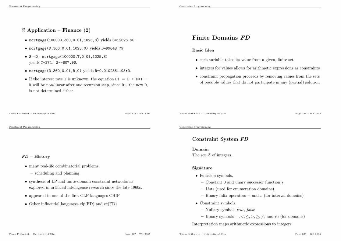
Constraint Programming
ℜ Application – Finance (2)
• mortgage(100000,360,0.01,1025,S) yields S=12625.90.
• mortgage(D,360,0.01,1025,0) yields D=99648.79.
• S=<0, mortgage(100000,T,0.01,1025,S)
yields T=374, S=-807.96.
• mortgage(D,360,0.01,R,0) yields R=0.0102861198*D.
• If the interest rate I is unknown, the equation D1 = D + D*I -
R will be non-linear after one recursion step, since D1, the new D,
is not determined either.
Thom Fruhwirth – University of Ulm Page 325 – WS 2005
Constraint Programming
Finite Domains FD
Basic Idea
• each variable takes its value from a given, finite set
• integers for values allows for arithmetic expressions as constraints
• constraint propagation proceeds by removing values from the sets
of possible values that do not participate in any (partial) solution
Thom Fruhwirth – University of Ulm Page 326 – WS 2005
Constraint Programming
FD – History
• many real-life combinatorial problems
– scheduling and planning
• synthesis of LP and finite-domain constraint networks as
explored in artificial intelligence research since the late 1960s.
• appeared in one of the first CLP languages CHIP
• Other influential languages clp(FD) and cc(FD)
Thom Fruhwirth – University of Ulm Page 327 – WS 2005
Constraint Programming
Constraint System FD
Domain
The set Z of integers.
Signature
• Function symbols.
– Constant 0 and unary successor function s
– Lists (used for enumeration domains)
– Binary infix operators + and .. (for interval domains)
• Constraint symbols.
– Nullary symbols true, false
– Binary symbols =, <,≤, >,≥, 6=, and in (for domains)
Interpretation maps arithmetic expressions to integers.
Thom Fruhwirth – University of Ulm Page 328 – WS 2005
Constraint Programming
Constraint System FD (2)
Allowed atomic constraints
Linear equations and inequations:
C ::= true false X in n..m X in [k1, . . . , kl] X⊙Y X+Y=Z
n, m, k1, . . . , kl: integers (l ≥ 0)
⊙ ∈ {=, <,>,≤,≥, 6=}X, Y and Z: pairwise distinct variables
domain constraint X in D: X ∈ D (D: given finite domain)
• enumeration domain constraint X in [k1, . . . , kl]:
values of X explicitly enumerated
• interval domain constraint X in n..m:
values of X in interval n..m (bounds included)
Thom Fruhwirth – University of Ulm Page 329 – WS 2005
Constraint Programming
Constraint System FD (3)
Constraint theory: Presburger Arithmetic
0 = s(X)→ ⊥X = X
X = Y → s(X) = s(Y )
s(X) = s(Y )→ X = Y
X = Y ∧ Y = Z → X = Z
X + 0 = X
X + s(Y ) = s(X + Y )
Decidable and complete CT for integer linear arithmetic.
Peano arithmetic adds ∗ and induction principle – incomplete.
Godel: Any consistent extension of Peano arithmetic is incomplete.
Thom Fruhwirth – University of Ulm Page 330 – WS 2005
Constraint Programming
Constraint System FD (4)
Constraint theory
Presburger’s arithmetic extended by
• 0 ≤ s(X), s(X) ≤ s(Y )↔ X ≤ Y , . . .
• X in n..m↔ n≤X ∧X≤m
• X in [k1, . . . , kl]↔ X=k1 ∨ . . . ∨X=kl
Empty domain X in [] or X in n..m with n > m is unsatisfiable.
Thom Fruhwirth – University of Ulm Page 331 – WS 2005
Constraint Programming
FD Interval vs. Enumeration Domain
Different implementations:
• interval domain
– constraint simplification performed only on interval bounds
• enumeration domain
– each element in the enumeration considered
– allow more simplification (tighter domains)
– only tractable for sufficiently small enumerations
Example:
• X in [1, 2, 3] ∧X 6=2 yields tighter domain constraint X in [1, 3]
• X in 1..3 ∧X 6=2: no propagation since interval bounds do not
change
Thom Fruhwirth – University of Ulm Page 332 – WS 2005
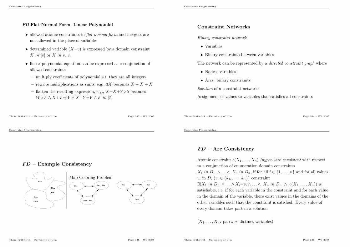
Constraint Programming
FD Flat Normal Form, Linear Polynomial
• allowed atomic constraints in flat normal form and integers are
not allowed in the place of variables
• determined variable (X=v) is expressed by a domain constraint
X in [v] or X in v..v.
• linear polynomial equation can be expressed as a conjunction of
allowed constraints
– multiply coefficients of polynomial s.t. they are all integers
– rewrite multiplications as sums, e.g., 3X becomes X +X +X
– flatten the resulting expression, e.g., X+X+Y >5 becomes
W>F ∧X+V=W ∧X+Y=V ∧ F in [5]
Thom Fruhwirth – University of Ulm Page 333 – WS 2005
Constraint Programming
Constraint Networks
Binary constraint network:
• Variables
• Binary constraints between variables
The network can be represented by a directed constraint graph where
• Nodes: variables
• Arcs: binary constraints
Solution of a constraint network:
Assignment of values to variables that satisfies all constraints
Thom Fruhwirth – University of Ulm Page 334 – WS 2005
Constraint Programming
FD – Example Consistency
Blau
Blau
Blau
Rot
Grün
Map Coloring Problem
Grün
Blau Blau Rot Rot Blau
Grün Blau
Thom Fruhwirth – University of Ulm Page 335 – WS 2005
Constraint Programming
FD – Arc Consistency
Atomic constraint c(X1, . . . , Xn) (hyper-)arc consistent with respect
to a conjunction of enumeration domain constraints
X1 in D1 ∧ . . .∧ Xn in Dn, if for all i ∈ {1, . . . , n} and for all values
vi in Di (vi ∈ {k1i, . . . , kli}) constraint
∃(X1 in D1 ∧ . . . ∧Xi=vi ∧ . . . ∧ Xn in Dn ∧ c(X1, . . . , Xn)) is
satisfiable, i.e. if for each variable in the constraint and for each value
in the domain of the variable, there exist values in the domains of the
other variables such that the constraint is satisfied. Every value of
every domain takes part in a solution
(X1, . . . , Xn: pairwise distinct variables)
Thom Fruhwirth – University of Ulm Page 336 – WS 2005
Constraint Programming
FD – Arc Consistency (2)
Logically, each domain is the projection of the constraints.
∃−Xi(c(X1, . . . , Xn) ∧X1 in D1 ∧ · · · ∧Xn in Dn)→ Xi in Di
A conjunction of constraints is arc consistent if each atomic
constraint in it is arc consistent.
Thom Fruhwirth – University of Ulm Page 337 – WS 2005
Constraint Programming
FD – Arc Consistency (3)
Examples:
• X in [1, 2, 3] ∧ X 6=2 not arc consistent
But: X in [1, 3] ∧X 6=2 arc consistent
• X in [1, 2, 3] ∧ Y in [1, 2, 3] ∧ X<Y not arc consistent
But: X in [1, 2] ∧ Y in [2, 3] ∧ X<Y arc consistent
Thom Fruhwirth – University of Ulm Page 338 – WS 2005
Constraint Programming
FD – Arc Consistency (4)
Limitations:
• must rename apart multiple occurrences of same variable
X 6=X represented by X 6=Y ∧X=Y
• arc consistency does not imply satisfiability (global consistency):
X in D ∧ Y in D ∧X 6=Y ∧X=Y arc consistent for all |D| > 1
• arc consistency sensitive to flattening:
X in [1, 2] ∧ Z in [2, 3, 4] ∧ 2X=Z not arc consistent
But:
X in [1, 2] ∧ Y in [1, 2] ∧ Z in [2, 3, 4] ∧ X=Y ∧ X+Y=Z
arc consistent
Thom Fruhwirth – University of Ulm Page 339 – WS 2005
Constraint Programming
FD – Arc Consistency (5)
Local Consistency Methods
Look at a small, fixed number of variables and constraints:
• Use them to propagate new, redundant constraints,
• Simplify the new constraints with old constraints
• Reconsider the changed old constraints until no more change
(fixpoint reached)
Local consistency (Propagation) + Search (Labeling, Enumeration)
= Complete Solver (Global consistency)
Thom Fruhwirth – University of Ulm Page 340 – WS 2005
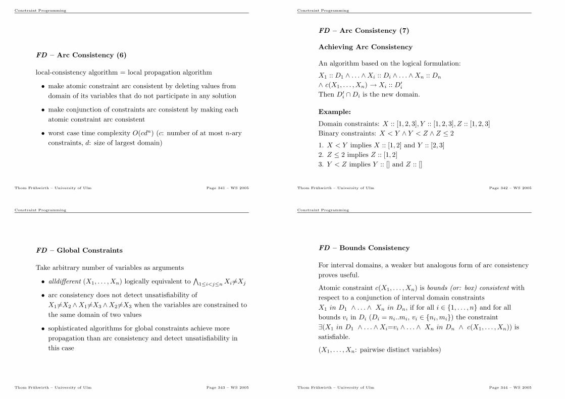
Constraint Programming
FD – Arc Consistency (6)
local-consistency algorithm = local propagation algorithm
• make atomic constraint arc consistent by deleting values from
domain of its variables that do not participate in any solution
• make conjunction of constraints arc consistent by making each
atomic constraint arc consistent
• worst case time complexity O(cdn) (c: number of at most n-ary
constraints, d: size of largest domain)
Thom Fruhwirth – University of Ulm Page 341 – WS 2005
Constraint Programming
FD – Arc Consistency (7)
Achieving Arc Consistency
An algorithm based on the logical formulation:
X1 :: D1 ∧ . . . ∧Xi :: Di ∧ . . . ∧Xn :: Dn
∧ c(X1, . . . , Xn) → Xi :: D′i
Then D′i ∩Di is the new domain.
Example:
Domain constraints: X :: [1, 2, 3], Y :: [1, 2, 3], Z :: [1, 2, 3]
Binary constraints: X < Y ∧ Y < Z ∧ Z ≤ 2
1. X < Y implies X :: [1, 2] and Y :: [2, 3]
2. Z ≤ 2 implies Z :: [1, 2]
3. Y < Z implies Y :: [] and Z :: []
Thom Fruhwirth – University of Ulm Page 342 – WS 2005
Constraint Programming
FD – Global Constraints
Take arbitrary number of variables as arguments
• alldifferent (X1, . . . , Xn) logically equivalent to∧
1≤i<j≤nXi 6=Xj
• arc consistency does not detect unsatisfiability of
X1 6=X2 ∧X1 6=X3 ∧X2 6=X3 when the variables are constrained to
the same domain of two values
• sophisticated algorithms for global constraints achieve more
propagation than arc consistency and detect unsatisfiability in
this case
Thom Fruhwirth – University of Ulm Page 343 – WS 2005
Constraint Programming
FD – Bounds Consistency
For interval domains, a weaker but analogous form of arc consistency
proves useful.
Atomic constraint c(X1, . . . , Xn) is bounds (or: box) consistent with
respect to a conjunction of interval domain constraints
X1 in D1 ∧ . . . ∧ Xn in Dn, if for all i ∈ {1, . . . , n} and for all
bounds vi in Di (Di = ni..mi, vi ∈ {ni,mi}) the constraint
∃(X1 in D1 ∧ . . . ∧Xi=vi ∧ . . . ∧ Xn in Dn ∧ c(X1, . . . , Xn)) is
satisfiable.
(X1, . . . , Xn: pairwise distinct variables)
Thom Fruhwirth – University of Ulm Page 344 – WS 2005
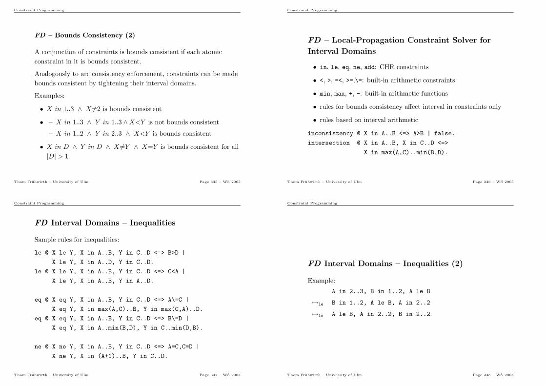
Constraint Programming
FD – Bounds Consistency (2)
A conjunction of constraints is bounds consistent if each atomic
constraint in it is bounds consistent.
Analogously to arc consistency enforcement, constraints can be made
bounds consistent by tightening their interval domains.
Examples:
• X in 1..3 ∧ X 6=2 is bounds consistent
• – X in 1..3 ∧ Y in 1..3 ∧X<Y is not bounds consistent
– X in 1..2 ∧ Y in 2..3 ∧ X<Y is bounds consistent
• X in D ∧ Y in D ∧ X 6=Y ∧ X=Y is bounds consistent for all
|D| > 1
Thom Fruhwirth – University of Ulm Page 345 – WS 2005
Constraint Programming
FD – Local-Propagation Constraint Solver for
Interval Domains
• in, le, eq, ne, add: CHR constraints
• <, >, =<, >=,\=: built-in arithmetic constraints
• min, max, +, -: built-in arithmetic functions
• rules for bounds consistency affect interval in constraints only
• rules based on interval arithmetic
inconsistency @ X in A..B <=> A>B | false.
intersection @ X in A..B, X in C..D <=>
X in max(A,C)..min(B,D).
Thom Fruhwirth – University of Ulm Page 346 – WS 2005
Constraint Programming
FD Interval Domains – Inequalities
Sample rules for inequalities:
le @ X le Y, X in A..B, Y in C..D <=> B>D |
X le Y, X in A..D, Y in C..D.
le @ X le Y, X in A..B, Y in C..D <=> C<A |
X le Y, X in A..B, Y in A..D.
eq @ X eq Y, X in A..B, Y in C..D <=> A\=C |
X eq Y, X in max(A,C)..B, Y in max(C,A)..D.
eq @ X eq Y, X in A..B, Y in C..D <=> B\=D |
X eq Y, X in A..min(B,D), Y in C..min(D,B).
ne @ X ne Y, X in A..B, Y in C..D <=> A=C,C=D |
X ne Y, X in (A+1)..B, Y in C..D.
Thom Fruhwirth – University of Ulm Page 347 – WS 2005
Constraint Programming
FD Interval Domains – Inequalities (2)
Example:
A in 2..3, B in 1..2, A le B
7→le B in 1..2, A le B, A in 2..2
7→le A le B, A in 2..2, B in 2..2.
Thom Fruhwirth – University of Ulm Page 348 – WS 2005
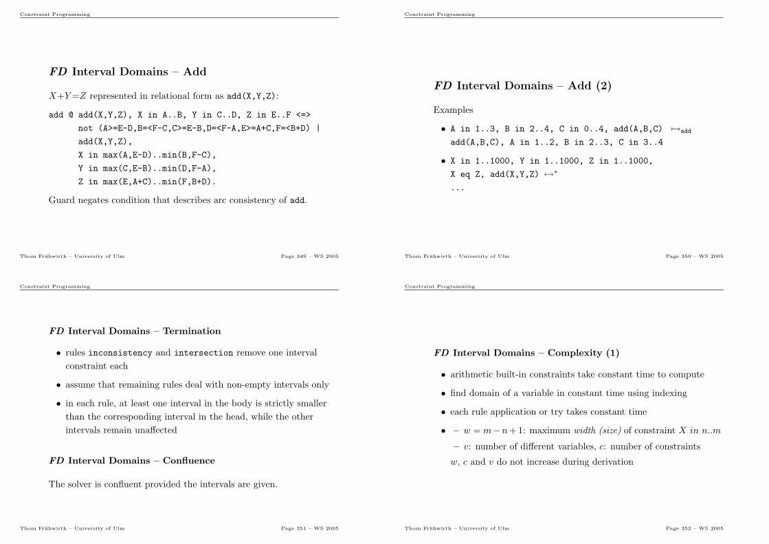
Constraint Programming
FD Interval Domains – Add
X+Y=Z represented in relational form as add(X,Y,Z):
add @ add(X,Y,Z), X in A..B, Y in C..D, Z in E..F <=>
not (A>=E-D,B=<F-C,C>=E-B,D=<F-A,E>=A+C,F=<B+D) |
add(X,Y,Z),
X in max(A,E-D)..min(B,F-C),
Y in max(C,E-B)..min(D,F-A),
Z in max(E,A+C)..min(F,B+D).
Guard negates condition that describes arc consistency of add.
Thom Fruhwirth – University of Ulm Page 349 – WS 2005
Constraint Programming
FD Interval Domains – Add (2)
Examples
• A in 1..3, B in 2..4, C in 0..4, add(A,B,C) 7→add
add(A,B,C), A in 1..2, B in 2..3, C in 3..4
• X in 1..1000, Y in 1..1000, Z in 1..1000,
X eq Z, add(X,Y,Z) 7→∗
...
Thom Fruhwirth – University of Ulm Page 350 – WS 2005
Constraint Programming
FD Interval Domains – Termination
• rules inconsistency and intersection remove one interval
constraint each
• assume that remaining rules deal with non-empty intervals only
• in each rule, at least one interval in the body is strictly smaller
than the corresponding interval in the head, while the other
intervals remain unaffected
FD Interval Domains – Confluence
The solver is confluent provided the intervals are given.
Thom Fruhwirth – University of Ulm Page 351 – WS 2005
Constraint Programming
FD Interval Domains – Complexity (1)
• arithmetic built-in constraints take constant time to compute
• find domain of a variable in constant time using indexing
• each rule application or try takes constant time
• – w = m−n+ 1: maximum width (size) of constraint X in n..m
– v: number of different variables, c: number of constraints
w, c and v do not increase during derivation
Thom Fruhwirth – University of Ulm Page 352 – WS 2005
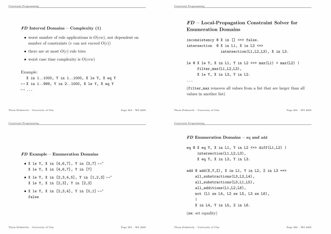
Constraint Programming
FD Interval Domains – Complexity (1)
• worst number of rule applications is O(vw), not dependent on
number of constraints (v can not exceed O(c))
• there are at most O(c) rule tries
• worst case time complexity is O(cvw)
Example:
X in 1..1000, Y in 1..1000, X le Y, X eq Y
7→ X in 1..999, Y in 2..1000, X le Y, X eq Y
7→ ...
Thom Fruhwirth – University of Ulm Page 353 – WS 2005
Constraint Programming
FD – Local-Propagation Constraint Solver for
Enumeration Domains
inconsistency @ X in [] <=> false.
intersection @ X in L1, X in L2 <=>
intersection(L1,L2,L3), X in L3.
le @ X le Y, X in L1, Y in L2 <=> max(L1) > max(L2) |
filter_max(L1,L2,L3),
X le Y, X in L3, Y in L2.
...
(filter_max removes all values from a list that are larger than all
values in another list)
Thom Fruhwirth – University of Ulm Page 354 – WS 2005
Constraint Programming
FD Example – Enumeration Domains
• X le Y, X in [4,6,7], Y in [3,7] 7→∗
X le Y, X in [4,6,7], Y in [7]
• X le Y, X in [2,3,4,5], Y in [1,2,3] 7→∗
X le Y, X in [2,3], Y in [2,3]
• X le Y, X in [2,3,4], Y in [0,1] 7→∗
false
Thom Fruhwirth – University of Ulm Page 355 – WS 2005
Constraint Programming
FD Enumeration Domains – eq and add
eq @ X eq Y, X in L1, Y in L2 <=> diff(L1,L2) |
intersection(L1,L2,L3),
X eq Y, X in L3, Y in L3.
add @ add(X,Y,Z), X in L1, Y in L2, Z in L3 ==>
all_substractions(L3,L2,L4),
all_substractions(L3,L1,L5),
all_additions(L1,L2,L6),
not (L1 se L4, L2 se L5, L3 se L6),
|
X in L4, Y in L5, Z in L6.
(se: set equality)
Thom Fruhwirth – University of Ulm Page 356 – WS 2005
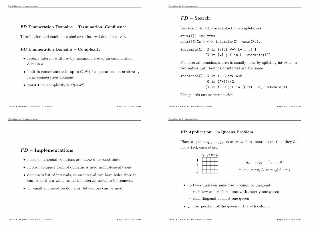
Constraint Programming
FD Enumeration Domains – Termination, Confluence
Termination and confluence similar to interval domain solver.
FD Enumeration Domains – Complexity
• replace interval width w by maximum size of an enumeration
domain d
• built-in constraints take up to O(d2) for operations on arbitrarily
large enumeration domains
• worst time complexity is O(cvd3)
Thom Fruhwirth – University of Ulm Page 357 – WS 2005
Constraint Programming
FD – Search
Use search to achieve satisfaction-completeness.
enum([]) <=> true.
enum([X|Xs]) <=> indomain(X), enum(Xs).
indomain(X), X in [V|L] <=> L=[_|_] |
(X in [V] ; X in L, indomain(X)).
For interval domains, search is usually done by splitting intervals in
two halves until bounds of interval are the same
indomain(X), X in A..B <=> A<B |
C is (A+B)//2,
(X in A..C ; X in (C+1)..B), indomain(X).
The guards ensure termination.
Thom Fruhwirth – University of Ulm Page 358 – WS 2005
Constraint Programming
FD – Implementations
• linear polynomial equations are allowed as constraints
• hybrid, compact form of domains is used in implementations
• domain is list of intervals, so an interval can have holes since it
can be split if a value inside the interval needs to be removed
• for small enumeration domains, bit vectors can be used
Thom Fruhwirth – University of Ulm Page 359 – WS 2005
Constraint Programming
FD Application – n-Queens Problem
Place n queens q1, . . . , qn on an n×n chess board, such that they do
not attack each other.
1234
q1 q2 q3 q4
q1, . . . , qn ∈ {1, . . . , n}∀ i6=j. qi 6=qj ∧ |qi − qj |6=|i− j|
• no two queens on same row, column or diagonal
– each row and each column with exactly one queen
– each diagonal at most one queen
• qi: row position of the queen in the i-th column
Thom Fruhwirth – University of Ulm Page 360 – WS 2005
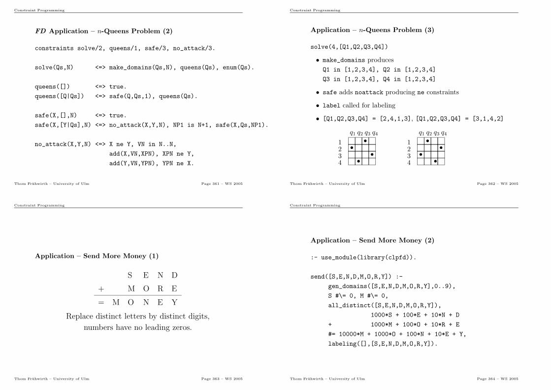
Constraint Programming
FD Application – n-Queens Problem (2)
constraints solve/2, queens/1, safe/3, no_attack/3.
solve(Qs,N) <=> make_domains(Qs,N), queens(Qs), enum(Qs).
queens([]) <=> true.
queens([Q|Qs]) <=> safe(Q,Qs,1), queens(Qs).
safe(X,[],N) <=> true.
safe(X,[Y|Qs],N) <=> no_attack(X,Y,N), NP1 is N+1, safe(X,Qs,NP1).
no_attack(X,Y,N) <=> X ne Y, VN in N..N,
add(X,VN,XPN), XPN ne Y,
add(Y,VN,YPN), YPN ne X.
Thom Fruhwirth – University of Ulm Page 361 – WS 2005
Constraint Programming
Application – n-Queens Problem (3)
solve(4,[Q1,Q2,Q3,Q4])
• make_domains produces
Q1 in [1,2,3,4], Q2 in [1,2,3,4]
Q3 in [1,2,3,4], Q4 in [1,2,3,4]
• safe adds noattack producing ne constraints
• label called for labeling
• [Q1,Q2,Q3,Q4] = [2,4,1,3], [Q1,Q2,Q3,Q4] = [3,1,4,2]
1234
••
••
q1 q2 q3 q4
1234
••
••
q1 q2 q3 q4
Thom Fruhwirth – University of Ulm Page 362 – WS 2005
Constraint Programming
Application – Send More Money (1)
S E N D
+ M O R E
= M O N E Y
Replace distinct letters by distinct digits,
numbers have no leading zeros.
Thom Fruhwirth – University of Ulm Page 363 – WS 2005
Constraint Programming
Application – Send More Money (2)
:- use_module(library(clpfd)).
send([S,E,N,D,M,O,R,Y]) :-
gen_domains([S,E,N,D,M,O,R,Y],0..9),
S #\= 0, M #\= 0,
all_distinct([S,E,N,D,M,O,R,Y]),
1000*S + 100*E + 10*N + D
+ 1000*M + 100*O + 10*R + E
#= 10000*M + 1000*O + 100*N + 10*E + Y,
labeling([],[S,E,N,D,M,O,R,Y]).
Thom Fruhwirth – University of Ulm Page 364 – WS 2005
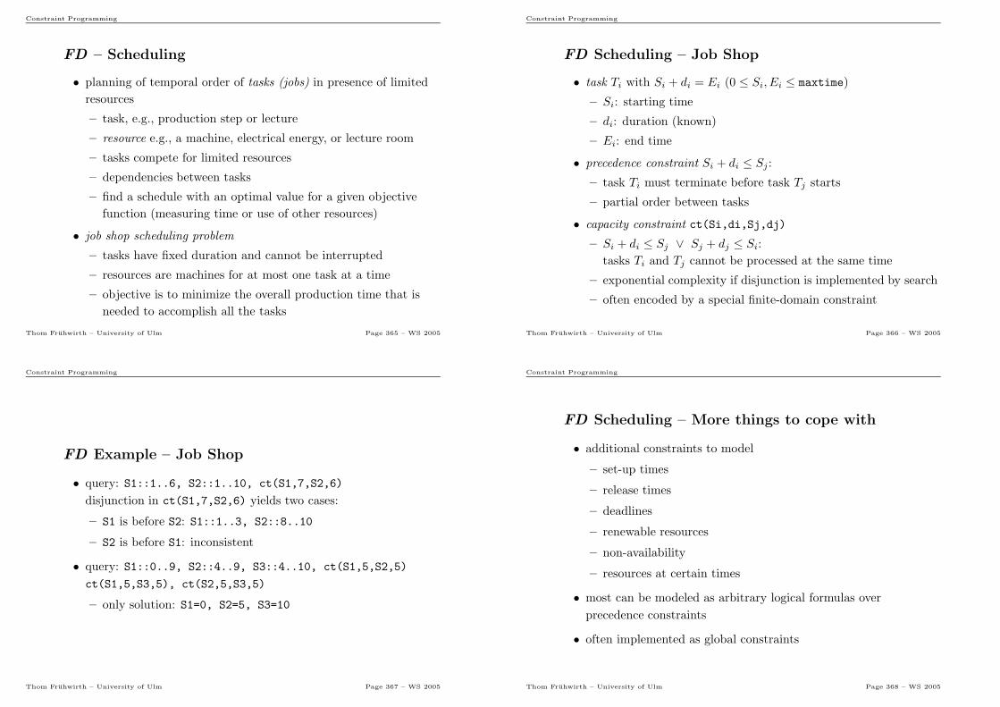
Constraint Programming
FD – Scheduling
• planning of temporal order of tasks (jobs) in presence of limited
resources
– task, e.g., production step or lecture
– resource e.g., a machine, electrical energy, or lecture room
– tasks compete for limited resources
– dependencies between tasks
– find a schedule with an optimal value for a given objective
function (measuring time or use of other resources)
• job shop scheduling problem
– tasks have fixed duration and cannot be interrupted
– resources are machines for at most one task at a time
– objective is to minimize the overall production time that is
needed to accomplish all the tasks
Thom Fruhwirth – University of Ulm Page 365 – WS 2005
Constraint Programming
FD Scheduling – Job Shop
• task Ti with Si + di = Ei (0 ≤ Si, Ei ≤ maxtime)
– Si: starting time
– di: duration (known)
– Ei: end time
• precedence constraint Si + di ≤ Sj :
– task Ti must terminate before task Tj starts
– partial order between tasks
• capacity constraint ct(Si,di,Sj,dj)
– Si + di ≤ Sj ∨ Sj + dj ≤ Si:
tasks Ti and Tj cannot be processed at the same time
– exponential complexity if disjunction is implemented by search
– often encoded by a special finite-domain constraint
Thom Fruhwirth – University of Ulm Page 366 – WS 2005
Constraint Programming
FD Example – Job Shop
• query: S1::1..6, S2::1..10, ct(S1,7,S2,6)
disjunction in ct(S1,7,S2,6) yields two cases:
– S1 is before S2: S1::1..3, S2::8..10
– S2 is before S1: inconsistent
• query: S1::0..9, S2::4..9, S3::4..10, ct(S1,5,S2,5)
ct(S1,5,S3,5), ct(S2,5,S3,5)
– only solution: S1=0, S2=5, S3=10
Thom Fruhwirth – University of Ulm Page 367 – WS 2005
Constraint Programming
FD Scheduling – More things to cope with
• additional constraints to model
– set-up times
– release times
– deadlines
– renewable resources
– non-availability
– resources at certain times
• most can be modeled as arbitrary logical formulas over
precedence constraints
• often implemented as global constraints
Thom Fruhwirth – University of Ulm Page 368 – WS 2005
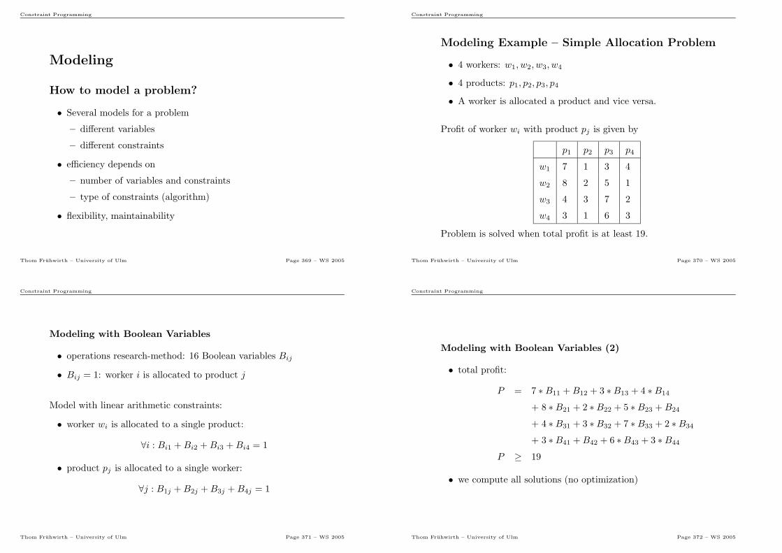
Constraint Programming
Modeling
How to model a problem?
• Several models for a problem
– different variables
– different constraints
• efficiency depends on
– number of variables and constraints
– type of constraints (algorithm)
• flexibility, maintainability
Thom Fruhwirth – University of Ulm Page 369 – WS 2005
Constraint Programming
Modeling Example – Simple Allocation Problem
• 4 workers: w1, w2, w3, w4
• 4 products: p1, p2, p3, p4
• A worker is allocated a product and vice versa.
Profit of worker wi with product pj is given by
p1 p2 p3 p4
w1 7 1 3 4
w2 8 2 5 1
w3 4 3 7 2
w4 3 1 6 3
Problem is solved when total profit is at least 19.
Thom Fruhwirth – University of Ulm Page 370 – WS 2005
Constraint Programming
Modeling with Boolean Variables
• operations research-method: 16 Boolean variables Bij
• Bij = 1: worker i is allocated to product j
Model with linear arithmetic constraints:
• worker wi is allocated to a single product:
∀i : Bi1 +Bi2 +Bi3 +Bi4 = 1
• product pj is allocated to a single worker:
∀j : B1j +B2j +B3j +B4j = 1
Thom Fruhwirth – University of Ulm Page 371 – WS 2005
Constraint Programming
Modeling with Boolean Variables (2)
• total profit:
P = 7 ∗B11 +B12 + 3 ∗B13 + 4 ∗B14
+ 8 ∗B21 + 2 ∗B22 + 5 ∗B23 +B24
+ 4 ∗B31 + 3 ∗B32 + 7 ∗B33 + 2 ∗B34
+ 3 ∗B41 +B42 + 6 ∗B43 + 3 ∗B44
P ≥ 19
• we compute all solutions (no optimization)
Thom Fruhwirth – University of Ulm Page 372 – WS 2005
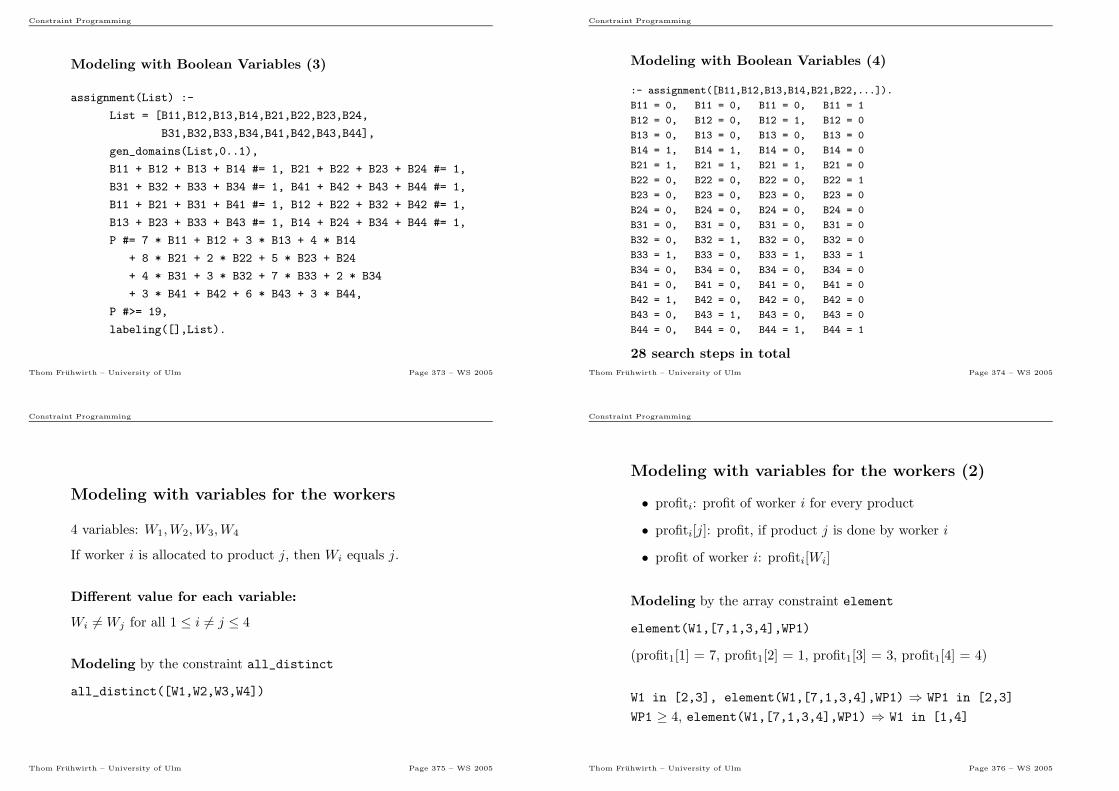
Constraint Programming
Modeling with Boolean Variables (3)
assignment(List) :-
List = [B11,B12,B13,B14,B21,B22,B23,B24,
B31,B32,B33,B34,B41,B42,B43,B44],
gen_domains(List,0..1),
B11 + B12 + B13 + B14 #= 1, B21 + B22 + B23 + B24 #= 1,
B31 + B32 + B33 + B34 #= 1, B41 + B42 + B43 + B44 #= 1,
B11 + B21 + B31 + B41 #= 1, B12 + B22 + B32 + B42 #= 1,
B13 + B23 + B33 + B43 #= 1, B14 + B24 + B34 + B44 #= 1,
P #= 7 * B11 + B12 + 3 * B13 + 4 * B14
+ 8 * B21 + 2 * B22 + 5 * B23 + B24
+ 4 * B31 + 3 * B32 + 7 * B33 + 2 * B34
+ 3 * B41 + B42 + 6 * B43 + 3 * B44,
P #>= 19,
labeling([],List).
Thom Fruhwirth – University of Ulm Page 373 – WS 2005
Constraint Programming
Modeling with Boolean Variables (4)
:- assignment([B11,B12,B13,B14,B21,B22,...]).
B11 = 0, B11 = 0, B11 = 0, B11 = 1
B12 = 0, B12 = 0, B12 = 1, B12 = 0
B13 = 0, B13 = 0, B13 = 0, B13 = 0
B14 = 1, B14 = 1, B14 = 0, B14 = 0
B21 = 1, B21 = 1, B21 = 1, B21 = 0
B22 = 0, B22 = 0, B22 = 0, B22 = 1
B23 = 0, B23 = 0, B23 = 0, B23 = 0
B24 = 0, B24 = 0, B24 = 0, B24 = 0
B31 = 0, B31 = 0, B31 = 0, B31 = 0
B32 = 0, B32 = 1, B32 = 0, B32 = 0
B33 = 1, B33 = 0, B33 = 1, B33 = 1
B34 = 0, B34 = 0, B34 = 0, B34 = 0
B41 = 0, B41 = 0, B41 = 0, B41 = 0
B42 = 1, B42 = 0, B42 = 0, B42 = 0
B43 = 0, B43 = 1, B43 = 0, B43 = 0
B44 = 0, B44 = 0, B44 = 1, B44 = 1
28 search steps in totalThom Fruhwirth – University of Ulm Page 374 – WS 2005
Constraint Programming
Modeling with variables for the workers
4 variables: W1,W2,W3,W4
If worker i is allocated to product j, then Wi equals j.
Different value for each variable:
Wi 6= Wj for all 1 ≤ i 6= j ≤ 4
Modeling by the constraint all_distinct
all_distinct([W1,W2,W3,W4])
Thom Fruhwirth – University of Ulm Page 375 – WS 2005
Constraint Programming
Modeling with variables for the workers (2)
• profiti: profit of worker i for every product
• profiti[j]: profit, if product j is done by worker i
• profit of worker i: profiti[Wi]
Modeling by the array constraint element
element(W1,[7,1,3,4],WP1)
(profit1[1] = 7, profit1[2] = 1, profit1[3] = 3, profit1[4] = 4)
W1 in [2,3], element(W1,[7,1,3,4],WP1) ⇒ WP1 in [2,3]
WP1 ≥ 4, element(W1,[7,1,3,4],WP1) ⇒ W1 in [1,4]
Thom Fruhwirth – University of Ulm Page 376 – WS 2005
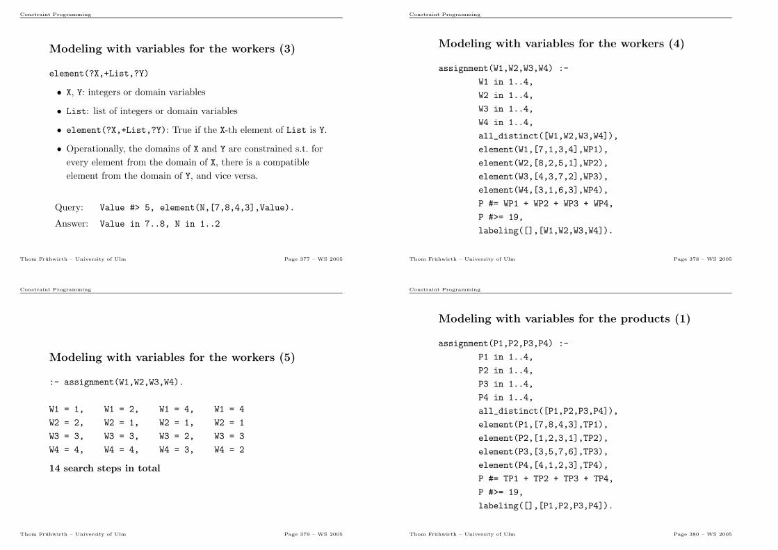
Constraint Programming
Modeling with variables for the workers (3)
element(?X,+List,?Y)
• X, Y: integers or domain variables
• List: list of integers or domain variables
• element(?X,+List,?Y): True if the X-th element of List is Y.
• Operationally, the domains of X and Y are constrained s.t. for
every element from the domain of X, there is a compatible
element from the domain of Y, and vice versa.
Query: Value #> 5, element(N,[7,8,4,3],Value).
Answer: Value in 7..8, N in 1..2
Thom Fruhwirth – University of Ulm Page 377 – WS 2005
Constraint Programming
Modeling with variables for the workers (4)
assignment(W1,W2,W3,W4) :-
W1 in 1..4,
W2 in 1..4,
W3 in 1..4,
W4 in 1..4,
all_distinct([W1,W2,W3,W4]),
element(W1,[7,1,3,4],WP1),
element(W2,[8,2,5,1],WP2),
element(W3,[4,3,7,2],WP3),
element(W4,[3,1,6,3],WP4),
P #= WP1 + WP2 + WP3 + WP4,
P #>= 19,
labeling([],[W1,W2,W3,W4]).
Thom Fruhwirth – University of Ulm Page 378 – WS 2005
Constraint Programming
Modeling with variables for the workers (5)
:- assignment(W1,W2,W3,W4).
W1 = 1, W1 = 2, W1 = 4, W1 = 4
W2 = 2, W2 = 1, W2 = 1, W2 = 1
W3 = 3, W3 = 3, W3 = 2, W3 = 3
W4 = 4, W4 = 4, W4 = 3, W4 = 2
14 search steps in total
Thom Fruhwirth – University of Ulm Page 379 – WS 2005
Constraint Programming
Modeling with variables for the products (1)
assignment(P1,P2,P3,P4) :-
P1 in 1..4,
P2 in 1..4,
P3 in 1..4,
P4 in 1..4,
all_distinct([P1,P2,P3,P4]),
element(P1,[7,8,4,3],TP1),
element(P2,[1,2,3,1],TP2),
element(P3,[3,5,7,6],TP3),
element(P4,[4,1,2,3],TP4),
P #= TP1 + TP2 + TP3 + TP4,
P #>= 19,
labeling([],[P1,P2,P3,P4]).
Thom Fruhwirth – University of Ulm Page 380 – WS 2005
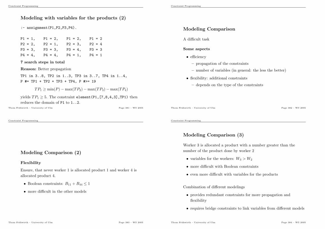
Constraint Programming
Modeling with variables for the products (2)
:- assignment(P1,P2,P3,P4).
P1 = 1, P1 = 2, P1 = 2, P1 = 2
P2 = 2, P2 = 1, P2 = 3, P2 = 4
P3 = 3, P3 = 3, P3 = 4, P3 = 3
P4 = 4, P4 = 4, P4 = 1, P4 = 1
7 search steps in total
Reason: Better propagation
TP1 in 3..8, TP2 in 1..3, TP3 in 3..7, TP4 in 1..4,
P #= TP1 + TP2 + TP3 + TP4, P #>= 19
TP1 ≥ min(P )−max(TP2)−max(TP3)−max(TP4)
yields TP1 ≥ 5. The constraint element(P1,[7,8,4,3],TP1) then
reduces the domain of P1 to 1..2.Thom Fruhwirth – University of Ulm Page 381 – WS 2005
Constraint Programming
Modeling Comparison
A difficult task
Some aspects
• efficiency
– propagation of the constraints
– number of variables (in general: the less the better)
• flexibility: additional constraints
– depends on the type of the constraints
Thom Fruhwirth – University of Ulm Page 382 – WS 2005
Constraint Programming
Modeling Comparison (2)
Flexibility
Ensure, that never worker 1 is allocated product 1 and worker 4 is
allocated product 4.
• Boolean constraints: B11 +B44 ≤ 1
• more difficult in the other models
Thom Fruhwirth – University of Ulm Page 383 – WS 2005
Constraint Programming
Modeling Comparison (3)
Worker 3 is allocated a product with a number greater than the
number of the product done by worker 2
• variables for the workers: W3 > W2
• more difficult with Boolean constraints
• even more difficult with variables for the products
Combination of different modelings
• provides redundant constraints for more propagation and
flexibility
• requires bridge constraints to link variables from different models
Thom Fruhwirth – University of Ulm Page 384 – WS 2005
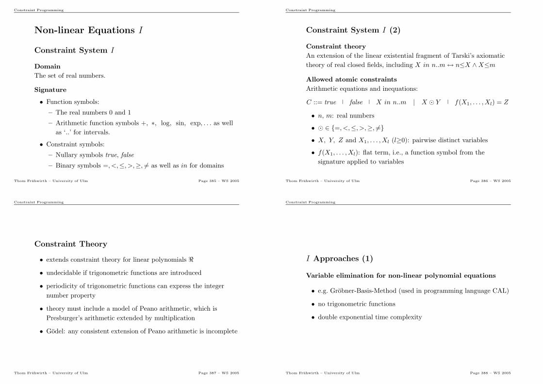
Constraint Programming
Non-linear Equations I
Constraint System I
Domain
The set of real numbers.
Signature
• Function symbols:
– The real numbers 0 and 1
– Arithmetic function symbols +, ∗, log, sin, exp, . . . as well
as ‘..’ for intervals.
• Constraint symbols:
– Nullary symbols true, false
– Binary symbols =, <,≤, >,≥, 6= as well as in for domains
Thom Fruhwirth – University of Ulm Page 385 – WS 2005
Constraint Programming
Constraint System I (2)
Constraint theory
An extension of the linear existential fragment of Tarski’s axiomatic
theory of real closed fields, including X in n..m↔ n≤X ∧X≤m
Allowed atomic constraints
Arithmetic equations and inequations:
C ::= true false X in n..m | X ⊙ Y f(X1, . . . , Xl) = Z
• n, m: real numbers
• ⊙ ∈ {=, <,≤, >,≥, 6=}• X, Y, Z and X1, . . . , Xl (l≥0): pairwise distinct variables
• f(X1, . . . , Xl): flat term, i.e., a function symbol from the
signature applied to variables
Thom Fruhwirth – University of Ulm Page 386 – WS 2005
Constraint Programming
Constraint Theory
• extends constraint theory for linear polynomials ℜ
• undecidable if trigonometric functions are introduced
• periodicity of trigonometric functions can express the integer
number property
• theory must include a model of Peano arithmetic, which is
Presburger’s arithmetic extended by multiplication
• Godel: any consistent extension of Peano arithmetic is incomplete
Thom Fruhwirth – University of Ulm Page 387 – WS 2005
Constraint Programming
I Approaches (1)
Variable elimination for non-linear polynomial equations
• e.g. Grobner-Basis-Method (used in programming language CAL)
• no trigonometric functions
• double exponential time complexity
Thom Fruhwirth – University of Ulm Page 388 – WS 2005
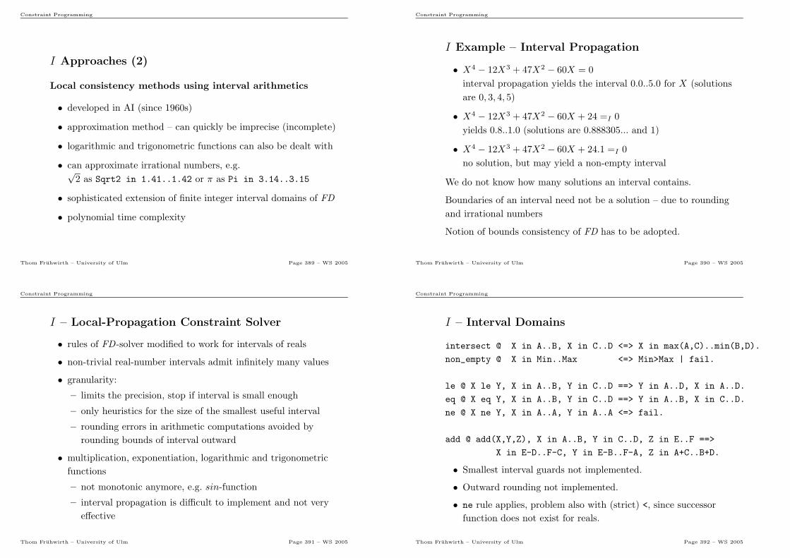
Constraint Programming
I Approaches (2)
Local consistency methods using interval arithmetics
• developed in AI (since 1960s)
• approximation method – can quickly be imprecise (incomplete)
• logarithmic and trigonometric functions can also be dealt with
• can approximate irrational numbers, e.g.√2 as Sqrt2 in 1.41..1.42 or π as Pi in 3.14..3.15
• sophisticated extension of finite integer interval domains of FD
• polynomial time complexity
Thom Fruhwirth – University of Ulm Page 389 – WS 2005
Constraint Programming
I Example – Interval Propagation
• X4 − 12X3 + 47X2 − 60X = 0
interval propagation yields the interval 0.0..5.0 for X (solutions
are 0, 3, 4, 5)
• X4 − 12X3 + 47X2 − 60X + 24 =I 0
yields 0.8..1.0 (solutions are 0.888305... and 1)
• X4 − 12X3 + 47X2 − 60X + 24.1 =I 0
no solution, but may yield a non-empty interval
We do not know how many solutions an interval contains.
Boundaries of an interval need not be a solution – due to rounding
and irrational numbers
Notion of bounds consistency of FD has to be adopted.
Thom Fruhwirth – University of Ulm Page 390 – WS 2005
Constraint Programming
I – Local-Propagation Constraint Solver
• rules of FD-solver modified to work for intervals of reals
• non-trivial real-number intervals admit infinitely many values
• granularity:
– limits the precision, stop if interval is small enough
– only heuristics for the size of the smallest useful interval
– rounding errors in arithmetic computations avoided by
rounding bounds of interval outward
• multiplication, exponentiation, logarithmic and trigonometric
functions
– not monotonic anymore, e.g. sin-function
– interval propagation is difficult to implement and not very
effective
Thom Fruhwirth – University of Ulm Page 391 – WS 2005
Constraint Programming
I – Interval Domains
intersect @ X in A..B, X in C..D <=> X in max(A,C)..min(B,D).
non_empty @ X in Min..Max <=> Min>Max | fail.
le @ X le Y, X in A..B, Y in C..D ==> Y in A..D, X in A..D.
eq @ X eq Y, X in A..B, Y in C..D ==> Y in A..B, X in C..D.
ne @ X ne Y, X in A..A, Y in A..A <=> fail.
add @ add(X,Y,Z), X in A..B, Y in C..D, Z in E..F ==>
X in E-D..F-C, Y in E-B..F-A, Z in A+C..B+D.
• Smallest interval guards not implemented.
• Outward rounding not implemented.
• ne rule applies, problem also with (strict) <, since successor
function does not exist for reals.
Thom Fruhwirth – University of Ulm Page 392 – WS 2005
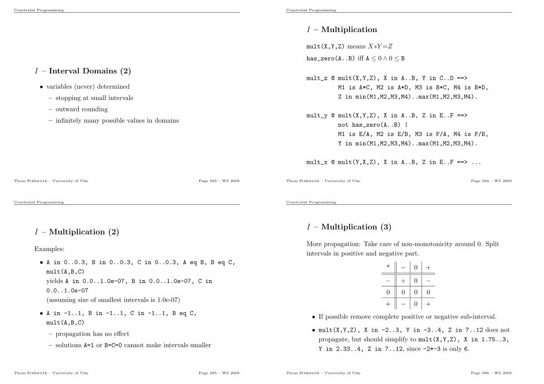
Constraint Programming
I – Interval Domains (2)
• variables (never) determined
– stopping at small intervals
– outward rounding
– infinitely many possible values in domains
Thom Fruhwirth – University of Ulm Page 393 – WS 2005
Constraint Programming
I – Multiplication
mult(X,Y,Z) means X∗Y=Z
has_zero(A..B) iff A ≤ 0 ∧ 0 ≤ B
mult_z @ mult(X,Y,Z), X in A..B, Y in C..D ==>
M1 is A*C, M2 is A*D, M3 is B*C, M4 is B*D,
Z in min(M1,M2,M3,M4)..max(M1,M2,M3,M4).
mult_y @ mult(X,Y,Z), X in A..B, Z in E..F ==>
not has_zero(A..B) |
M1 is E/A, M2 is E/B, M3 is F/A, M4 is F/B,
Y in min(M1,M2,M3,M4)..max(M1,M2,M3,M4).
mult_x @ mult(Y,X,Z), X in A..B, Z in E..F ==> ...
Thom Fruhwirth – University of Ulm Page 394 – WS 2005
Constraint Programming
I – Multiplication (2)
Examples:
• A in 0..0.3, B in 0..0.3, C in 0..0.3, A eq B, B eq C,
mult(A,B,C)
yields A in 0.0..1.0e-07, B in 0.0..1.0e-07, C in
0.0..1.0e-07
(assuming size of smallest intervals is 1.0e-07)
• A in -1..1, B in -1..1, C in -1..1, B eq C,
mult(A,B,C)
– propagation has no effect
– solutions A=1 or B=C=0 cannot make intervals smaller
Thom Fruhwirth – University of Ulm Page 395 – WS 2005
Constraint Programming
I – Multiplication (3)
More propagation: Take care of non-monotonicity around 0. Split
intervals in positive and negative part.
* − 0 +
− + 0 −0 0 0 0
+ − 0 +
• If possible remove complete positive or negative sub-interval.
• mult(X,Y,Z), X in -2..3, Y in -3..4, Z in 7..12 does not
propagate, but should simplify to mult(X,Y,Z), X in 1.75..3,
Y in 2.33..4, Z in 7..12, since -2*-3 is only 6.
Thom Fruhwirth – University of Ulm Page 396 – WS 2005
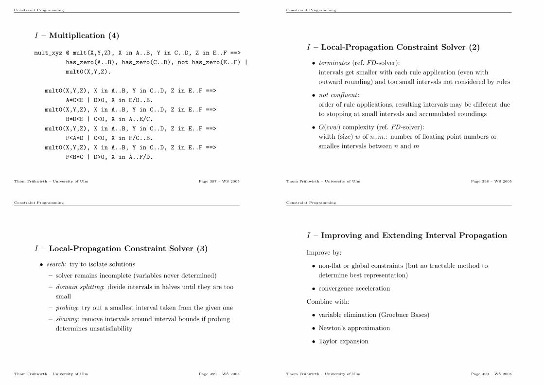
Constraint Programming
I – Multiplication (4)
mult_xyz @ mult(X,Y,Z), X in A..B, Y in C..D, Z in E..F ==>
has_zero(A..B), has_zero(C..D), not has_zero(E..F) |
mult0(X,Y,Z).
mult0(X,Y,Z), X in A..B, Y in C..D, Z in E..F ==>
A*C<E | D>0, X in E/D..B.
mult0(X,Y,Z), X in A..B, Y in C..D, Z in E..F ==>
B*D<E | C<0, X in A..E/C.
mult0(X,Y,Z), X in A..B, Y in C..D, Z in E..F ==>
F<A*D | C<0, X in F/C..B.
mult0(X,Y,Z), X in A..B, Y in C..D, Z in E..F ==>
F<B*C | D>0, X in A..F/D.
Thom Fruhwirth – University of Ulm Page 397 – WS 2005
Constraint Programming
I – Local-Propagation Constraint Solver (2)
• terminates (ref. FD-solver):
intervals get smaller with each rule application (even with
outward rounding) and too small intervals not considered by rules
• not confluent :
order of rule applications, resulting intervals may be different due
to stopping at small intervals and accumulated roundings
• O(cvw) complexity (ref. FD-solver):
width (size) w of n..m.: number of floating point numbers or
smalles intervals between n and m
Thom Fruhwirth – University of Ulm Page 398 – WS 2005
Constraint Programming
I – Local-Propagation Constraint Solver (3)
• search: try to isolate solutions
– solver remains incomplete (variables never determined)
– domain splitting: divide intervals in halves until they are too
small
– probing: try out a smallest interval taken from the given one
– shaving: remove intervals around interval bounds if probing
determines unsatisfiability
Thom Fruhwirth – University of Ulm Page 399 – WS 2005
Constraint Programming
I – Improving and Extending Interval Propagation
Improve by:
• non-flat or global constraints (but no tractable method to
determine best representation)
• convergence acceleration
Combine with:
• variable elimination (Groebner Bases)
• Newton’s approximation
• Taylor expansion
Thom Fruhwirth – University of Ulm Page 400 – WS 2005

Constraint Programming
I – Applications
• physics, chemistry, mathematics (geometry)
• physical, chemical, and molecular-biological modeling and
simulation of hybrid systems
• hybrid circuits, spatial reasoning, robot control, equilibrium of
chemicals, financial analysis
Thom Fruhwirth – University of Ulm Page 401 – WS 2005